Summertime M2 Internal Tides in the Northern Yellow Sea

The summertime M₂ internal tide in the northern Yellow Sea is investigated with moored current meter observations and numerical current model results. The hydrodynamic model, which is implemented from the Regional Ocean Model System (ROMS) with 1 km horizontal resolution, is capable of resolving the internal tidal dynamics and the results are validated in a comparison with observations. The vertical pattern of a mode-1, semi-diurnal internal tide is clearly captured by the moored ADCP as well as in the simulation results. Spectral analysis of the current results shows that the M₂ internal tide is dominant in the northern Yellow Sea. Analysis of the major M₂ internal tide energetics demonstrated a complex spatial pattern. The tidal mixing front along the Korean coast and on the northern shelf provided proper conditions for the generation and propagation of the internal tides. Near the Changshan islands, the M₂ internal tide is mainly generated near the local topography anomalies with relatively strong current magnitude, equal to about 30% of the barotropic component, thus modifying the local current field. These local internal tides are short-lived phenomena rapidly being dissipated along the propagation pathway, restricting their influence within a few kilometers around the islands.

Introduction

Waves in the ocean are a dominant part of the dynamics. Especially visible are wind driven high frequency surface waves and low frequency tides. Less visible though are internal waves, existing in stratified water masses. However, internal waves are a potential source for ocean mixing and can be important for material transportation. When tidal currents flow over steep topography such as ridges or continental shelf breaks, internal waves with tidal frequency can be generated, known as internal tides. Our present work originates from an observation of currents in the water column near Changshan islands, and the results reveal a clear two-layered oscillation superposed on the strong semi-diurnal tide which characterizes the currents in the region. This internal wave will obviously modify the total current in the area. Knowledge of the currents here is particularly useful since this is an important area for scallop aquaculture.

The Yellow Sea (Figure 1A) is the marginal sea between the mainland of China and the Korean peninsula. According to Egbert and Ray (2001), Yellow Sea is estimated to have the most intensive tidal energy dissipation due to friction from shallow topography estimated to be about 150 GW annually. Affected by strong tides and the East Asian monsoon system, the hydrodynamics of the Yellow Sea have high spatial-temporal variability (Hwang et al., 2014). The competition between the solar radiation induced buoyancy and the endless tidal mixing power, creates the featured summertime “Yellow Sea bottom cold water” (YSBCW) located in the central region of the Yellow Sea surrounded by the tidal mixing front (Lin et al., 2019). The tidal mixing front is usually located between the 20–60 m isobaths with relatively homogeneous water inshore and stratified water offshore (Tana et al., 2017; Zhu et al., 2017; Lin et al., 2019). The stratified waters enable the generation and propagation of baroclinic waves, including the internal tides. Compared to the research conducted in the South China Sea, where the Luzon strait act as a powerful wave generator of internal waves with amplitude up to hundred meters (Jan et al., 2008; Shang et al., 2015; Yan et al., 2020), internal dynamics in the Yellow Sea have been less investigated. For a coastal region with activities such as fishing and aquaculture, knowledge on the coastal circulation and internal tidal-induced hydrodynamics will be important.

FIGURE 1

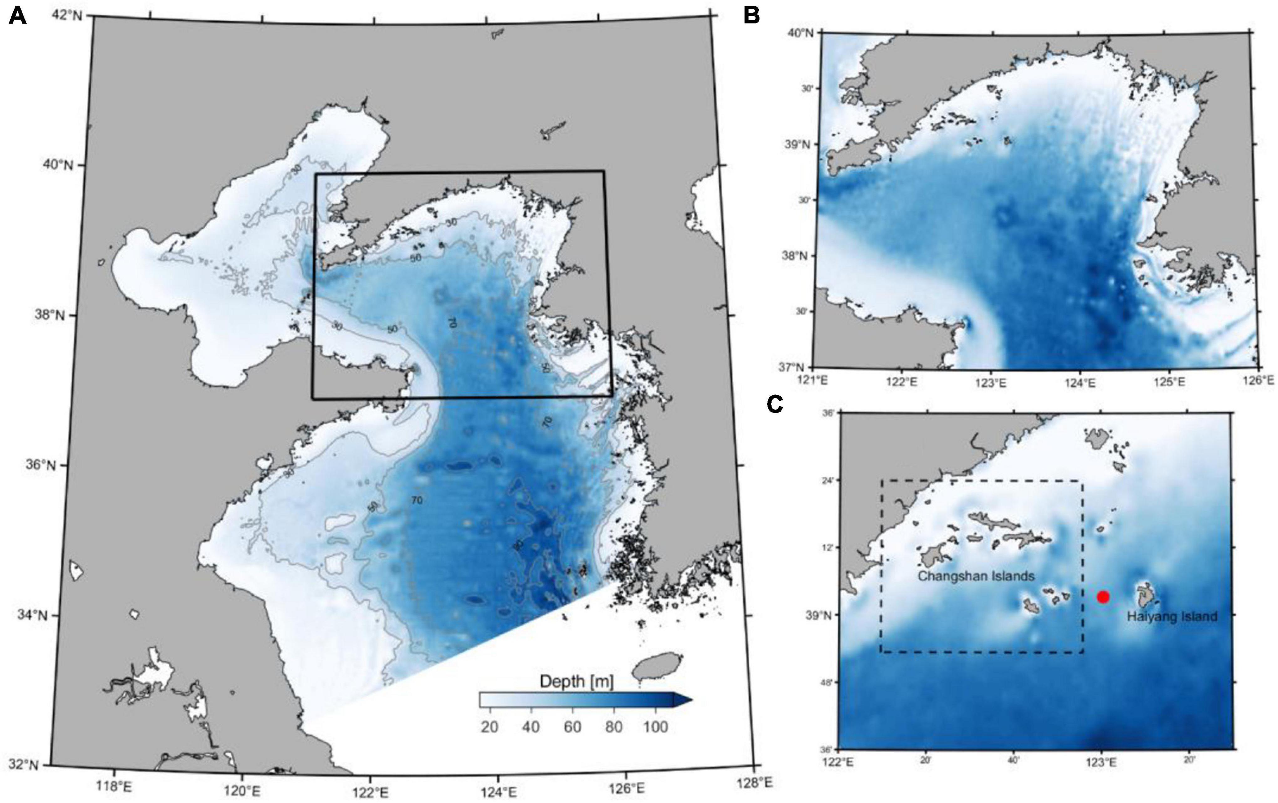
Figure 1. Domain and topography of the Yellow Sea model. (A) Model domain covering the Yellow Sea and Bohai Sea. (B) Major results will be presented from the northern Yellow Sea where the ADCP mooring site is shown as the red dot in (C). All the subfigures share the same color scale as shown in (A).

Previous literature on the internal tides in the Yellow Sea is mainly derived from observations and mainly for the southern part where the water depth exceeds 80 m, and the stratification is established throughout the year (Lee et al., 2006; Liu et al., 2009; Wei et al., 2013). Liu et al. (2019) have studied the characteristics of the M₂ internal tide in the Yellow Sea at basin scale with a numerical model, concluding with complicated spatial interference wave patterns and strong seasonality. During summer, the M₂ internal tide is generated from multiple sources and the baroclinic kinetic energy is present as the stratification is established around the YSBCW. The major baroclinic energy input is distributed in the southern Yellow Sea near the Yangtze River estuary and the shelf break near Jeju Island. In winter, the spatial coverage of the internal tides usually become very limited (Liu et al., 2019). There were also few reports of the internal tides in the northern Yellow Sea from in-situ observations. Guo and Hu (2010) reported the observed regular oscillation of the isotherms at the semi-diurnal frequency off the Qingdao coast, which is originated from the M₂ internal tide. Wang et al. (2020) identified the mode-1, semi-diurnal internal tides with moored current profiler and temperature/conductivity sensors off the coast of Shandong Peninsula and concluded with a significant internal tidal induced cross-shore advection of the coastal mass transport. However, knowledge and data regarding the internal tides on the northern shelf of the Yellow Sea can barely be found.

During the summer of 2017, an RDI ADCP profiling current meter was placed at the bottom on the northern shelf of the Yellow Sea near the Changshan islands (Figure 1C). From these observations, a clear mode-1 vertical baroclinic oscillation with a semi-diurnal period was seen, indicating a semi-diurnal internal tide passing the mooring location. In our study, we combined results from a numerical current model and the observations to investigate the dynamics of the M₂ internal tides on the northern shelf of the Yellow Sea in summer (Figure 1B). The objective of this study is to clarify the generation, propagation, and dissipation characteristic of the internal tides and to demonstrate their impact on local hydrodynamics in the northern Yellow Sea. We find that the mode-1, semi-diurnal internal tide will increase the total current in the bottom layers in the Changshan islands area where the water masses are stratified during summer. The internal waves are generated locally and with limited regional propagation. The content of this paper is organized as follows: The model setup, observation, and the analysis method are described in section “Materials and Methods.” In section “Results,” the results including the current observations, the simulated internal tide field, and corresponding energetics, are given. In section “Discussion,” the model performance will be evaluated and the internal tidal dynamics in the northern Yellow Sea will be discussed. Finally, a conclusion will be summarized in section “Conclusion.”

Materials and Methods

Model Setup

The model implemented for this study is based on the Regional Ocean Modeling System (ROMS), which is a free surface, terrain-following, primitive equations, hydrostatic ocean model on an Arakawa-C grid (Shchepetkin and McWilliams, 2005; Haidvogel et al., 2008). A detailed description of the model implementation for the Yellow Sea can be found in Lin et al. (2019). The model covers the Yellow Sea and the Bohai Sea with the horizontal grid size being ∼1 km with 40 vertical layers derived with the stretching factors 7.0 and 2.0, and with a minimum depth of 15 m, giving enhanced resolution near the surface and the bottom. As the horizontal wavelength of internal tides is usually far larger than the water depth on the northern shelf, a hydrostatic model is applicable to resolve the internal tides with the 1 km model horizontal resolution. The model bathymetry is interpolated from SRTM30-plus shuttle radar altimetry supplemented with side-scan sonar survey data and the GEBCO 30” database (Becker et al., 2009). The model is configured with the Generic Length Scale k-kl vertical mixing scheme (Warner et al., 2005).

A full model set up with realistic forcing and boundary conditions was conducted. The atmospheric forcing is taken from the European Centre for Medium-Range Weather Forecast ERA-Interim Reanalysis datasets (Dee et al., 2011), with the net heat flux computed from a bulk formulae by Fairall et al. (1996). The daily mean values of elevation, momentum, water temperature, and salinity were obtained from the HYCOM daily global ocean reanalysis and interpolated to the model grid as open boundary conditions. Eleven tidal components from the Oregon State University global inverse tidal model of TPXO7.2 (Egbert and Erofeeva, 2002) were specified at the open boundary. Open boundary data are imposed with a radiative-nudging scheme and a quadratic bottom drag was employed with the friction coefficient of 0.0025 applied to the entire model domain. A simulation of the period from August 2013 to December 2018 was conducted, and the results from the summertime of 2017 will be used in this study.

Additionally, two simulations were conducted covering the period July–August 2017 in order to investigate the spatial-temporal characteristics of the dominant M₂ internal tide of the northern Yellow Sea. The first is a barotropic simulation with homogeneous water which eliminates the baroclinic component and with the M₂ tide as the only forcing at the open boundary. The second simulation is conducted with the same forcing setup but with the monthly mean stratification extracted from the climatological simulation results. The results will be used to demonstrate the internal tidal dynamics. The model configurations are listed in Table 1.

TABLE 1

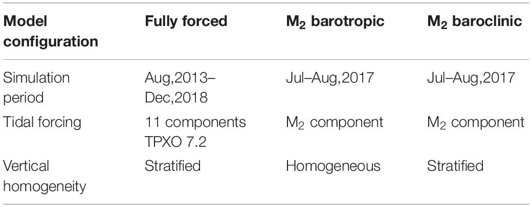
Table 1. The configurations of the model simulations used in the study.

Observations

An RDI acoustic doppler current profiler (1.0 MHz, bin size 2.0 m, 20 bins) was moored at the bottom near Changshan islands from July 10 to August 24, 2017. The accuracy of the instrument is 1% measured value ± 0.5 cm/s for current profiling, ± 0.1 for the integrated temperature sensor, and 0.5% of maximum range for the pressure sensor. The deployment location is shown in Figure 1C. The instrument was moored at the seafloor measuring upwards with a range of about 40 m. The sampling interval was set to 10 min. The water depth at the mooring location is approximately 40 m, and the water pressure time series was recorded with an integrated pressure sensor.

The horizontal baroclinic current velocity u′(z,t) will be extracted from both the observation and simulation results, by subtracting the depth-averaged barotropic component from the total current as:

$u^{{}^{\prime }}(z,t)=u(z,t)-\frac{1}{h}{\int }_{-h}^{0}u(z,t)\mathit{d}z$

where h is the water depth and u(z,t) is the total velocity. A 4-h lowpass filter is applied to eliminate higher-frequency signals.

Harmonic analysis will be applied to both the barotropic and baroclinic flows to obtain the current ellipses of the M₂ component. Spectral analysis is also applied to the horizontal baroclinic current velocity at different depths to demonstrate the vertical power spectrum distribution.

Generation and Energetics of the Internal Tides

The generation of internal tide requires a stratified water column and a barotropic tide that manages to perturb this stratification. In a situation with a sloping bottom, generation of internal tidal waves from the M₂ constituent can be described by a functional relation between the M₂ tidal wave frequency (ω), the local inertial frequency (the Coriolis parameter, f), the local buoyancy frequency (N), and the local slope of bottom topography (s, dimensionless) defined as vertical depth change over unit horizontal grid length (Thorpe, 1998; Cacchione et al., 2002). The inertial frequency can be calculated as f = 2Ωsin(φ), where Ω is the angular velocity of Earth rotation and φ is the local latitude. On the northern shelf of the Yellow Sea, the local inertial frequency is within the range of 1.36–1.48 × 10^–5 s^–1.

A characteristic angle of the M₂ internal tide (β) can be expressed as:

$\mathrm{\beta }=\sqrt{\frac{{\mathrm{\omega }}^2-f^2}{N^2-{\mathrm{\omega }}^2}}(1)$

and the functional relation between this characteristic angle and the topographical slope is calculated as:

$\mathrm{\gamma }=\frac{s}{\mathrm{\beta }}\mathit{\hspace{1em}\hspace{1em}\hspace{1em}\hspace{1em}\hspace{1em}\hspace{1em}\hspace{1em}}(2)$

A critical slope is when γ < 1, subcritical for γ = 1, and supercritical for γ > 1. In areas around a critical slope, the internal wave beam angle matches the topographic slope and internal tide generation is most favorable. The generated internal waves can propagate to shallower regions with subcritical slope or being reflected at the supercritical slope (Thorpe, 1998; Cacchione et al., 2002).

Liu et al. (2019) have computed the seasonal M₂ internal tide energetics in the whole Yellow Sea using an energy conversion rate (C) from barotropic to baroclinic motion calculated as:

$C=W\cdot p^{\prime }(3)$

where W is the vertical barotropic velocity induced by horizontal barotropic flow over topography:

$W=-{\nabla }_H\left[\left(h+\mathrm{\eta }\right)U_H\right].(4)$

Here U_H is the horizontal barotropic flow, h is the bottom depth, and η is the sea surface elevation. In this study, the conversion rate will be calculated with the M₂ baroclinic simulation results, and will be integrated over the water depth and averaged over 32 semi-diurnal tidal cycles in the simulation period from July 26 to August 10, 2017.

The perturbation pressure p′ is derived from the perturbation density ρ′. According to the definition of Kang and Fringer (2012), the perturbation density can be calculated as:

${\rho }^{\prime }=\rho (z,t)-{\rho }_0-{\rho }_b\left(z\right)(5)$

where ρ(z,t) is the time-dependent density of the water column, ρ₀ is the reference density (ρ₀ = 1,000 kg/m³), and ρ_b(z) is the time-independent background density. The perturbation pressure is then calculated as:

$p^{\prime }=g{\int }_z^{\mathrm{\eta }}{\rho }^{\prime }\mathit{d}z.(6)$

In the expression for the energy conversion rate C, a positive value means that W and p′ are in phase and the local barotropic energy is transferred to baroclinic energy. A negative value of C may imply a superposition of local and remote internal tides and the barotropic-baroclinic conversion does not happen (Carter et al., 2012; Kang and Fringer, 2012; Masunaga et al., 2017). This metric has been widely used in previous studies to understand the internal tidal dynamics in coastal regions (Kang and Fringer, 2012; Nash et al., 2012; Kumar et al., 2019; Liu et al., 2019).

The depth-integrated baroclinic energy flux can be computed from current model results according to Kang and Fringer (2012) as:

$F_{bc}={\int }_{-h}^{\mathrm{\eta }}{p}^{\prime }{u}^{\prime }\mathit{d}z(7)$

where u′ is the horizontal baroclinic current component. The depth-integrated baroclinic energy flux will also be averaged over 32 semi-diurnal tidal cycles in the simulation period from July 26 to August 10, 2017.

Coherent-Incoherent Analysis of Tidal Waves

According to Nash et al. (2012), a broadband internal tide can be decomposed into two components, (1) the coherent component, which is largely predictable and can be described by a series of tidal frequency sinusoids, and (2) the incoherent component, which is largely unpredictable and associated with intermittent pulses of tidal-band energy that are arriving with different phases and amplitudes. The coherent component of the internal tides is often applied as a parameter to estimate the contribution of local generation from the barotropic tides (Nash et al., 2012; Kumar et al., 2019; Li et al., 2020).

The coherent-incoherent analysis can be applied to time series from, e.g., observations or current model results. The harmonic analysis based on the least-squares method will be used to obtain the semi-diurnal internal tidal currents of the M₂, N₂, S₂ constituents, which will be tested as coherent variables that are phase-locked with the local barotropic tides. A fourth-order Butterworth filter will be applied to extract the baroclinic current of the semi-diurnal frequency band (1.73∼2.13 cpd) from the observation and the simulation results. The coherent internal tidal current is then subtracted, and the remaining signal within the semi-diurnal band can be defined as incoherent.

To demonstrate the baroclinic energy contribution of the locally and remotely generated internal tides, the observed and simulated currents with full forcing were decomposed to coherent and incoherent components of the semi-diurnal tidal constituents M₂, S₂, K₂, and N₂. The horizontal kinetic energy is then computed as $\text{KE}=\frac{1}{2}{\mathrm{\rho }}_0\left[u^2+v^2\right]$, where u,v are the horizontal velocity component and ρ₀ is the reference density.

Results

Currents Around the Changshan Islands in the Northern Yellow Sea

The measured and modeled horizontal velocities at different depths are shown to basically flow along the coastline isobaths with the major oscillation direction about 30–210 degrees (Figure 2). The model results compare reasonably well with the observations in both magnitude and oscillation direction. The observed current magnitudes are 0.69, 0.86, and 0.96 m/s for the depth of 5, 15, and 30 m, respectively. The corresponding model results are 0.71, 0.91, and 1.08 m/s. The root-mean-square error of observed and simulated currents are 0.09, 0.10, and 0.16 m/s for the presented layers. For both the observation and the simulation, the flow becomes stronger toward the bottom. This vertical structure indicates that the contribution from baroclinic components of the current can be of importance in the mooring region.

FIGURE 2

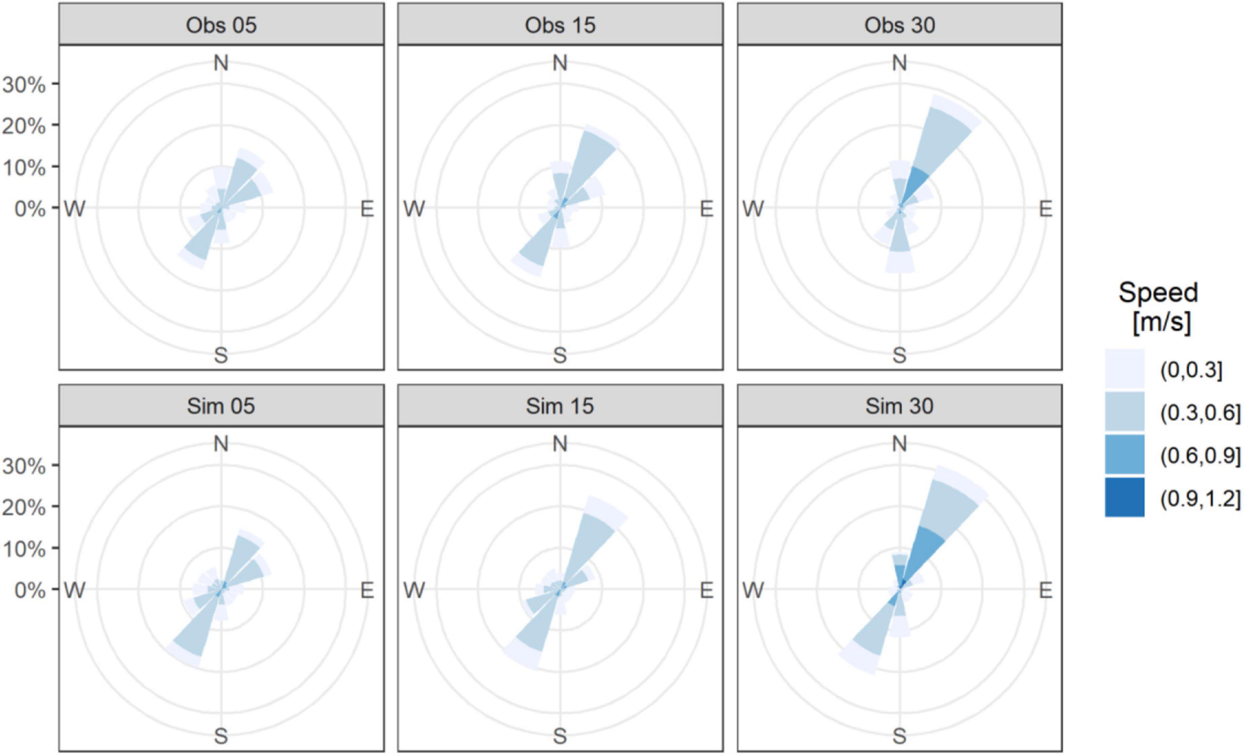
Figure 2. Current directions and magnitudes from the observed (top) and simulated (bottom) total current at different depths (5, 15, and 30 m below surface).

The mean density at the surface (Figure 3a) and bottom (Figure 3b) water for July 2017, illustrates a thermal front approximately located between the 20–60 m isobaths, since in July the water temperature is sufficiently high for the temperature to be the leading factor in the determination of water density. Inshore of this front is homogeneous coastal water and offshore is stratified water (Figure 3). The ADCP was moored near the cold/heavy water boundary or the thermal front area. The background stratification enables the propagation of baroclinic waves with frequencies between the local inertial frequency (f) and the buoyancy frequency (N).

FIGURE 3

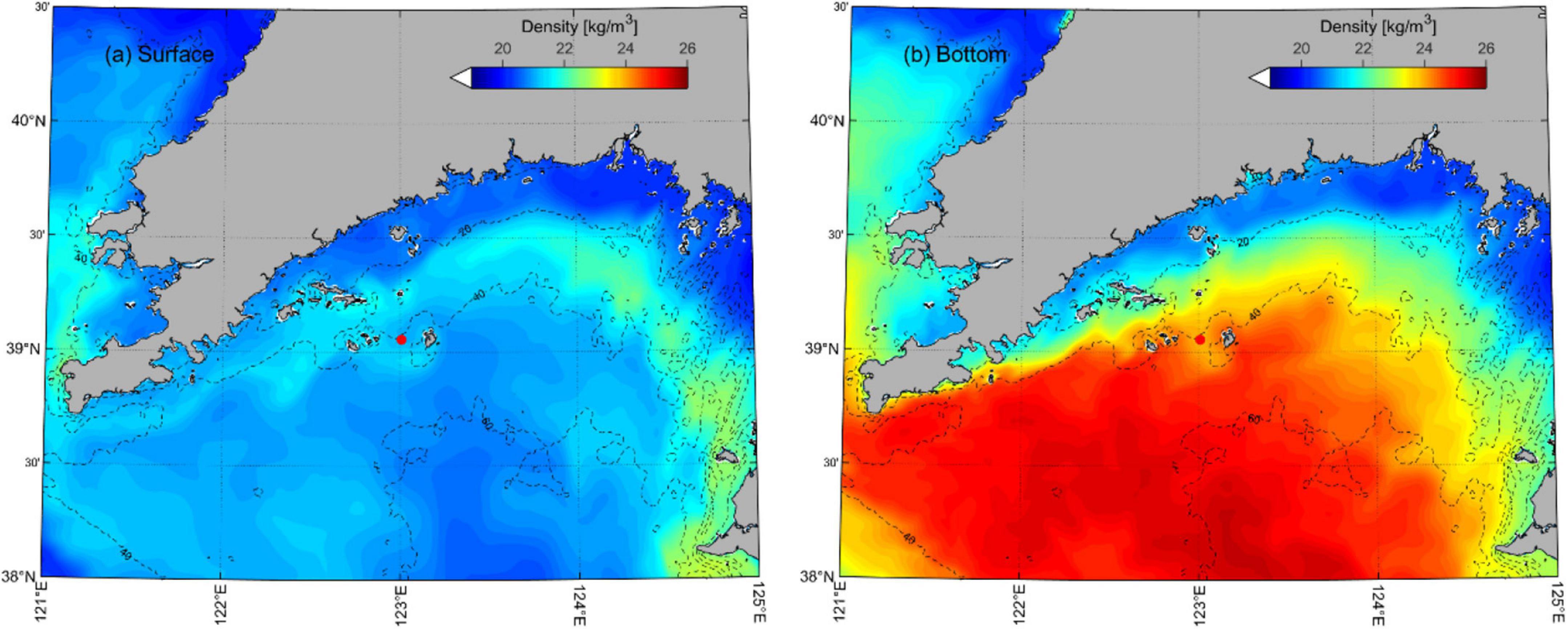
Figure 3. (a) Surface and (b) bottom density (kg/m³) computed from the numerical model results for July 2017. The dashed lines represent the isobath contours of 20, 40, and 60 m. The ADCP mooring site is shown with the red dot.

To illustrate the vertical structure of the baroclinic flow, the baroclinic current along the major axis 30–210° with the positive values toward 30°is extracted (Figures 4a,b). The data from above 10 m is excluded due to the impact of the surface wind. The vertical structure of the measured baroclinic velocity profile is a typical mode-1 plane internal wave with a clear semi-diurnal period, implying a dominating semi-diurnal internal tidal signal. The current model results are comparable to the observation with a similar vertical structure and current magnitude. The amplitudes of both measured and simulated baroclinic currents are around 0.2 m/s, indicating that the baroclinic component speed is comparable to the barotropic.

FIGURE 4

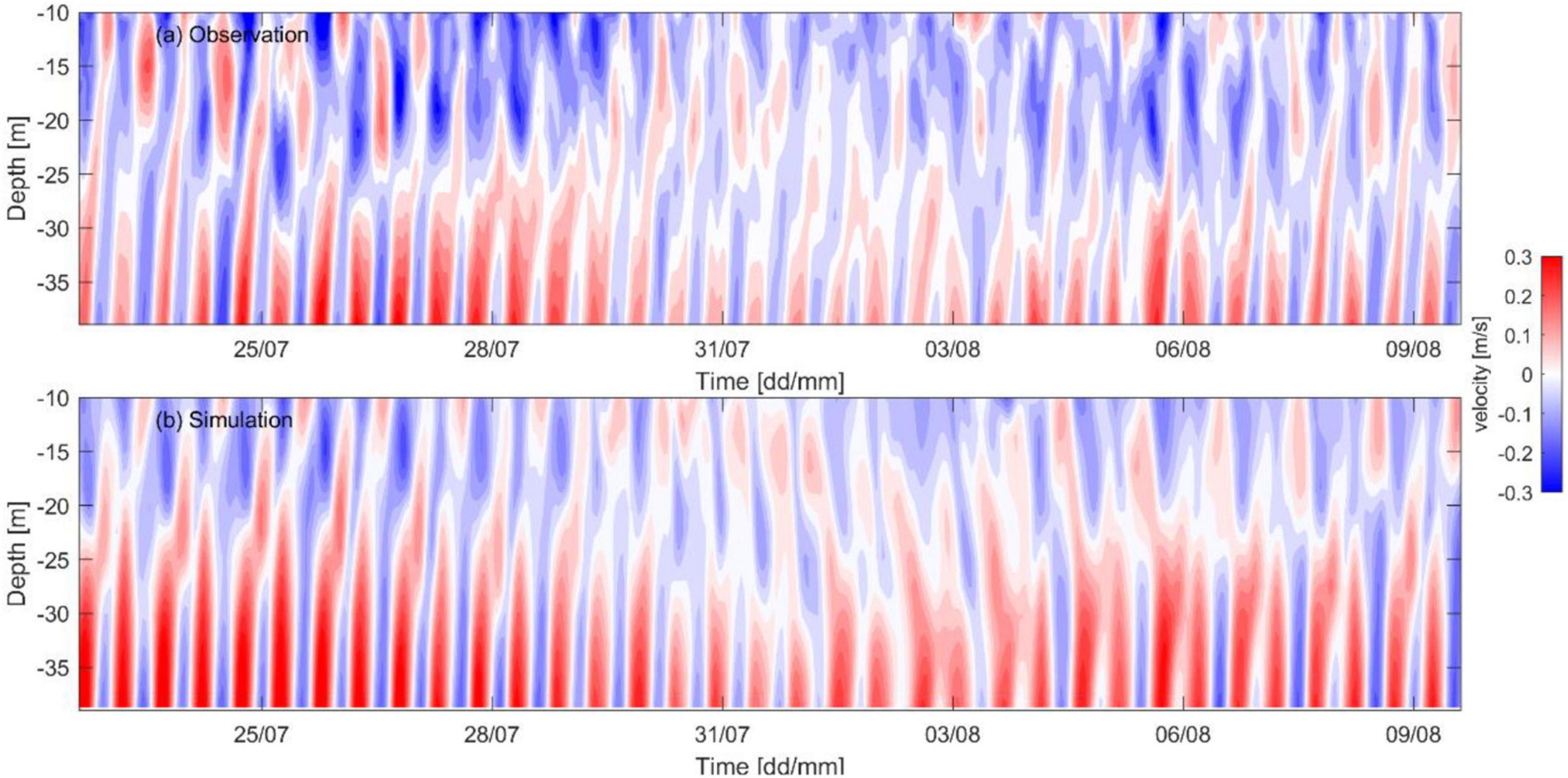
Figure 4. The filtered baroclinic current component below 10 m depth for (a) observation and (b) simulation at the mooring site from July 23 to August 10, 2017. The component is computed along the major axis of the flow, which have the positive values at 30°toward north-east.

The observed and simulated M₂ current ellipses of both the barotropic and baroclinic flow are presented in Figures 5A,B. The modeled barotropic M₂ tidal ellipse is a bit stretched along the major axis in the numerical model results compared to the observation, but the orientation of the ellipses matches well and is roughly along the isobaths (Figure 5A). The magnitude of the barotropic M₂ tidal current is around 0.4 m/s, which is comparable to both the observation and simulation results. Figure 5B shows the baroclinic M₂ tidal ellipse distribution for both observation and simulation results. The baroclinic M₂ currents have a nearly opposite phase between the surface and bottom layers, representing the feature of the mode-1 wave. The simulation results reproduce the baroclinic M₂ ellipse for the upper layers, while the current magnitudes are slightly overestimated in the lower layers. The maximum baroclinic M₂ current speed is around 0.1 m/s for both observed and simulated results.

FIGURE 5

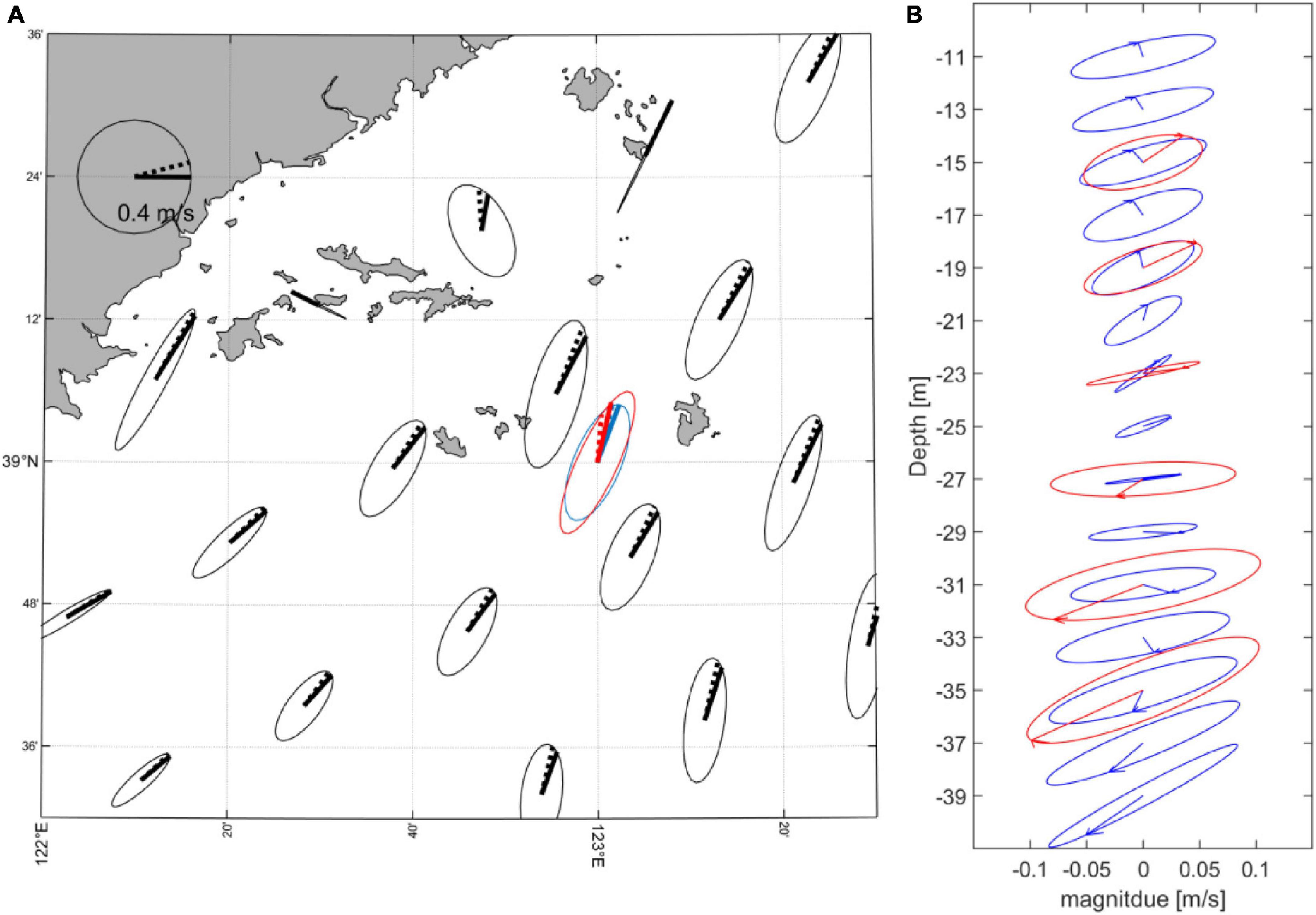
Figure 5. (A) The barotropic M2 tidal ellipse derived from the model results (black), the ADCP observation (blue), and the simulation results at the mooring site (red) for 2017. (B) The vertical baroclinic M2 tidal ellipse derived from ADCP mooring results (blue) and the simulated ellipses (red) at given depths.

To further investigate the baroclinic currents near the mooring location, the vertical spectra is derived for the water column between 5 and ∼35 m depth (Figures 6a,b). The baroclinic vertical spectra computed from the ADCP measurement (Figure 6a) is relatively complicated, with various smaller energy contributions at different depths and frequencies. However, for the whole water column, the energy is mainly distributed around the semi-diurnal bandwidth, especially the M₂ tidal frequency. The modeled baroclinic signal (Figure 6b) has a similar vertical structure for the whole water column, and the energy is concentrated near the semi-diurnal M₂ component.

FIGURE 6

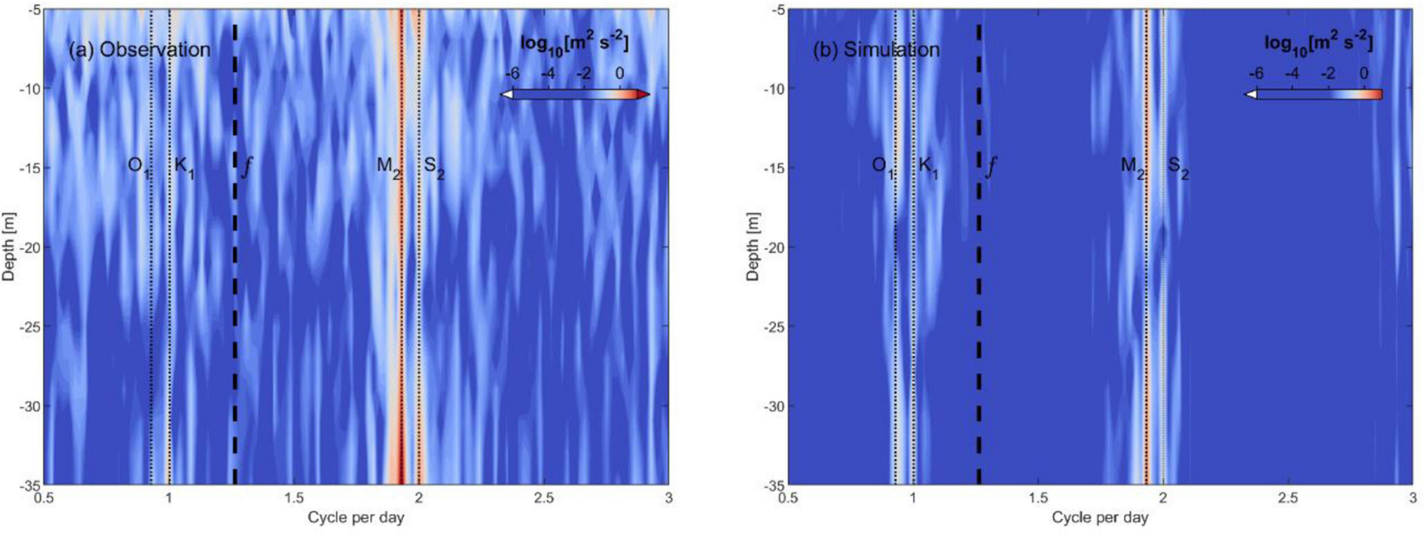
Figure 6. Spectral analysis results of (a) observed and (b) simulated baroclinic current at the mooring site. The diurnal constituents K₁, O_1, and semi-diurnal constituents M₂, S₂ are represented with vertical dotted lines, and the inertial frequency (f) is represented with the thick dotted line.

The vertically averaged KE of the band-passed barotropic and coherent/incoherent baroclinic tides are presented in Figures 7A,B for the current observation. Figure 7A illustrates that the barotropic tide is the dominant current component at the mooring location. The variability of the coherent semi-diurnal baroclinic tides is largely correlated with the variability of the barotropic tide, as shown in Figure 7B. The incoherent baroclinic KE during the observation period is much weaker compared to the barotropic KE. The time-averaged semi-diurnal barotropic KE is 67 J/m³ at the mooring site, and the corresponding baroclinic KE is only 4 J/m³. The energy of the coherent baroclinic tides is also much larger than the incoherent baroclinic tide, and accounts for almost 83% of the total semi-diurnal baroclinic KE. A similar analysis is also applied to the model results (figure not shown). The model overestimates the semi-diurnal barotropic motion, with a time-averaged KE being 80 J/m³, and the corresponding baroclinic KE is estimated to be 10 J/m³. The fraction between coherent and incoherent semi-diurnal baroclinic KE is consistent with the observations though, being around 85%.

FIGURE 7

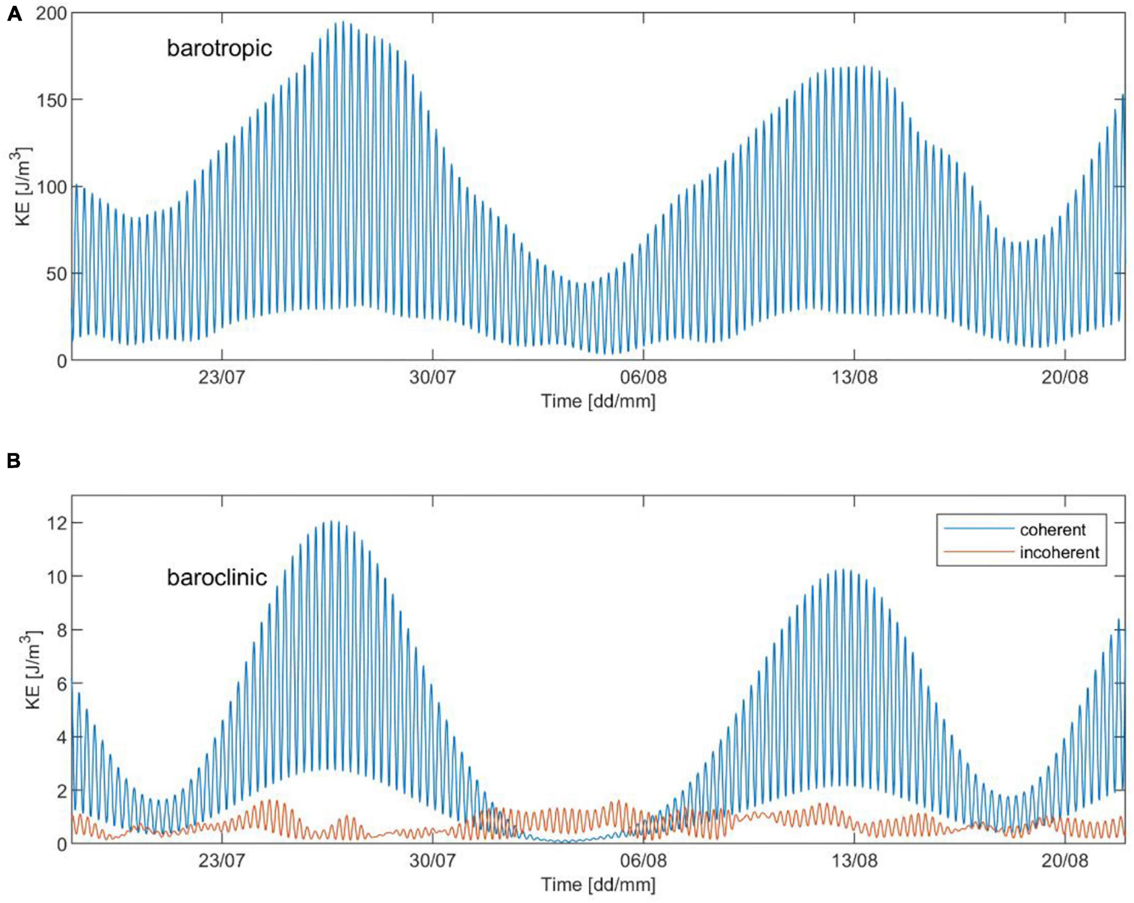
Figure 7. Vertically averaged kinetic energy of the band-passed observed horizontal velocity. (A) The barotropic horizontal kinetic energy. (B) The coherent and incoherent baroclinic horizontal kinetic energy.

To demonstrate the impact of the locally generated internal tide on the current field in the region around the Changshan islands, the simulated baroclinic current velocities at different depths are shown in Figures 8A–D, together with the barotropic flow shown in Figures 8E,F. The current is extracted from the M₂ baroclinic simulation on July 23, with a 6-h time difference between the columns. Figure 8 clearly shows the M₂ barotropic current is dominant, although the internal tidal current cannot be neglected around the Changshan islands. The statistics of the flow speed are shown in Table 2. The internal tidal current is stronger near the islands in the deeper part, close to the generation site (Figures 8C,D). Furthermore, there is an apparent direction change of the current, representing an opposite phase of the internal tidal current. The statistics of the current speed at 15 m depth are similar to that of the deeper flows, but the current field is more uniformly distributed for the upper layer (Table 2 and Figures 8A,B). The mean flow speed of the internal tidal current accounts for about 30% of the barotropic current at each presented layer, and the flow modification on the barotropic tide will be more pronounced closer to the islands.

FIGURE 8

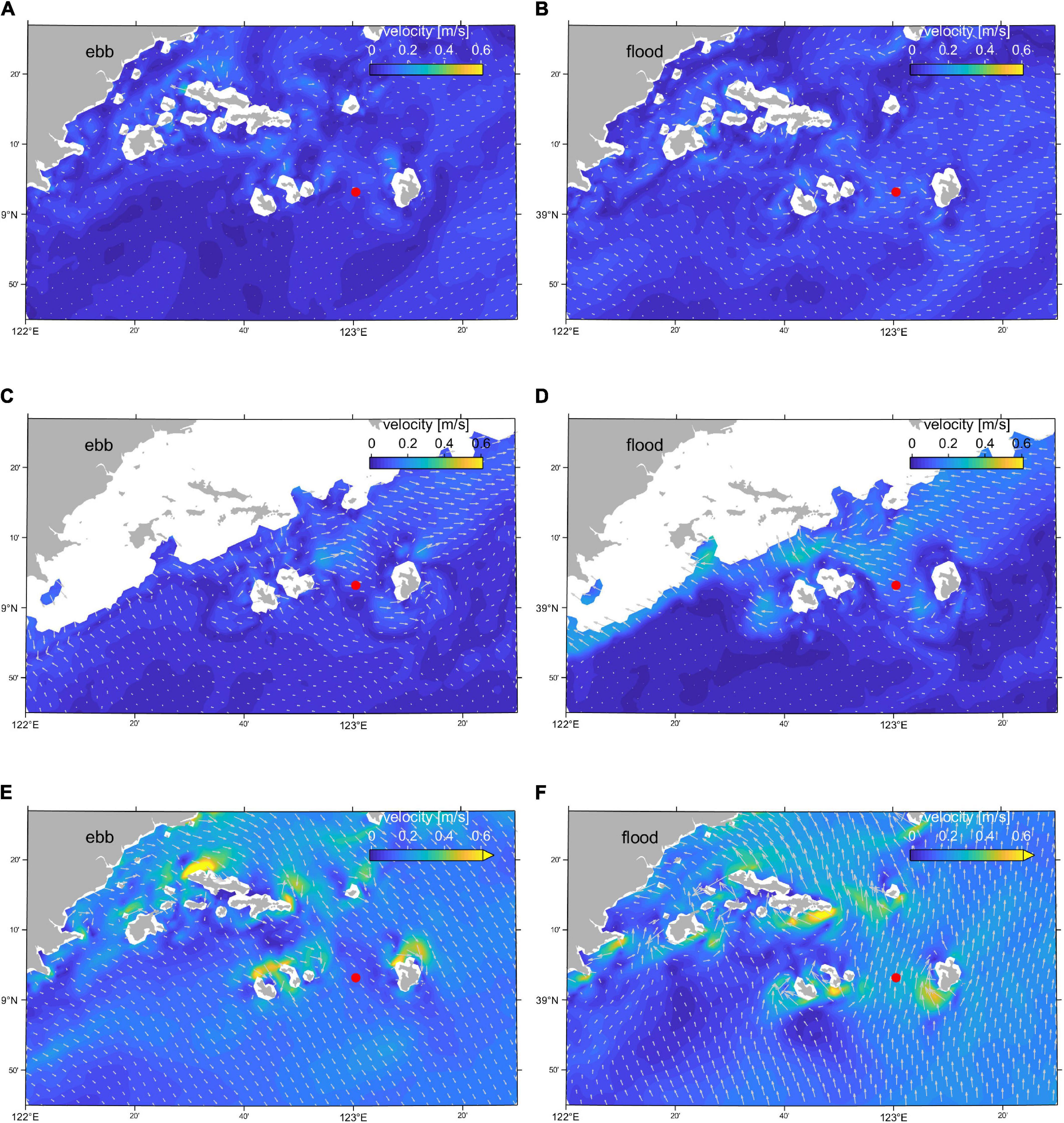
Figure 8. Modeled M₂ baroclinic flow for horizontal current fields (m/s) 6-h apart (at ebb tide and flood tide) at different depths. (A,B) Baroclinic current at 15 m depth. (C,D) Baroclinic current at 30 m depth. (E,F) Barotropic flow. The baroclinic current component will add (or subtract) to the total current. The ADCP mooring location is marked as a red dot.

TABLE 2

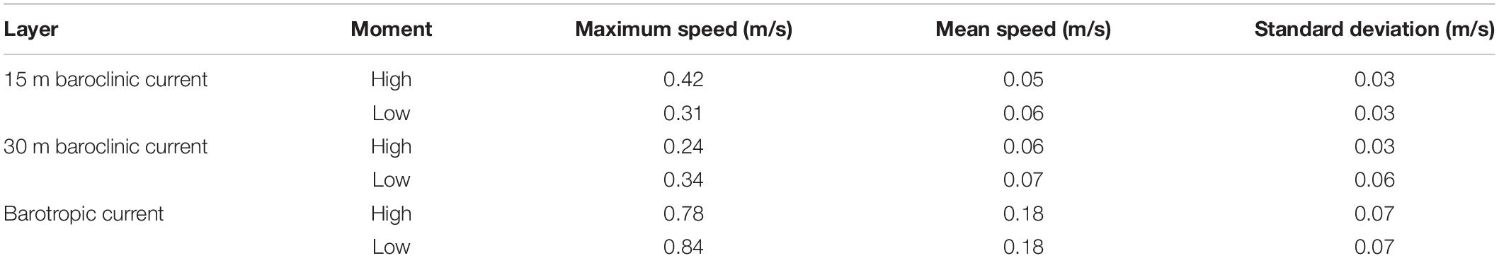
Table 2. Statistics of current speed around the Changshan islands in Figure 8.

The M₂ Internal Tide in the Northern Yellow Sea

With the summertime stratification and strong tidal current in the northern Yellow Sea, we expect favorable conditions for generation and propagation of internal tides. A measure of where internal tide generation might occur is the slope criticality (γ) for the M₂ internal tide (computed from Equation 2). The spatial distribution of the critical slope values in the northern Yellow Sea is shown in Figure 9A. The topographic angle is derived from the model bathymetry, and the near bottom buoyancy frequency is derived and averaged from the modeled density profiles for a tidal period during July 26 to August 10, 2017. The critical slopes (γ = 1) are mostly confined within the isobaths between ∼40 and ∼60 m, which overlap the location of the tidal mixing front (Figure 3). Areas of supercritical slopes will reflect the waves, while the waves can propagate in areas of sub-critical slopes depending on the local stratification. The rugged topography along the Korean coast has near critical or supercritical slope values, acting as an internal tide generator. Near the Changshan islands, there are also critical slopes that are eligible for emitting M₂ internal tides (Figure 9B). The depth-mean slope criticality from the model shows that favorable generation sites for M₂ internal tides are generally located between the depths of 40∼60 m (Figure 9C).

FIGURE 9

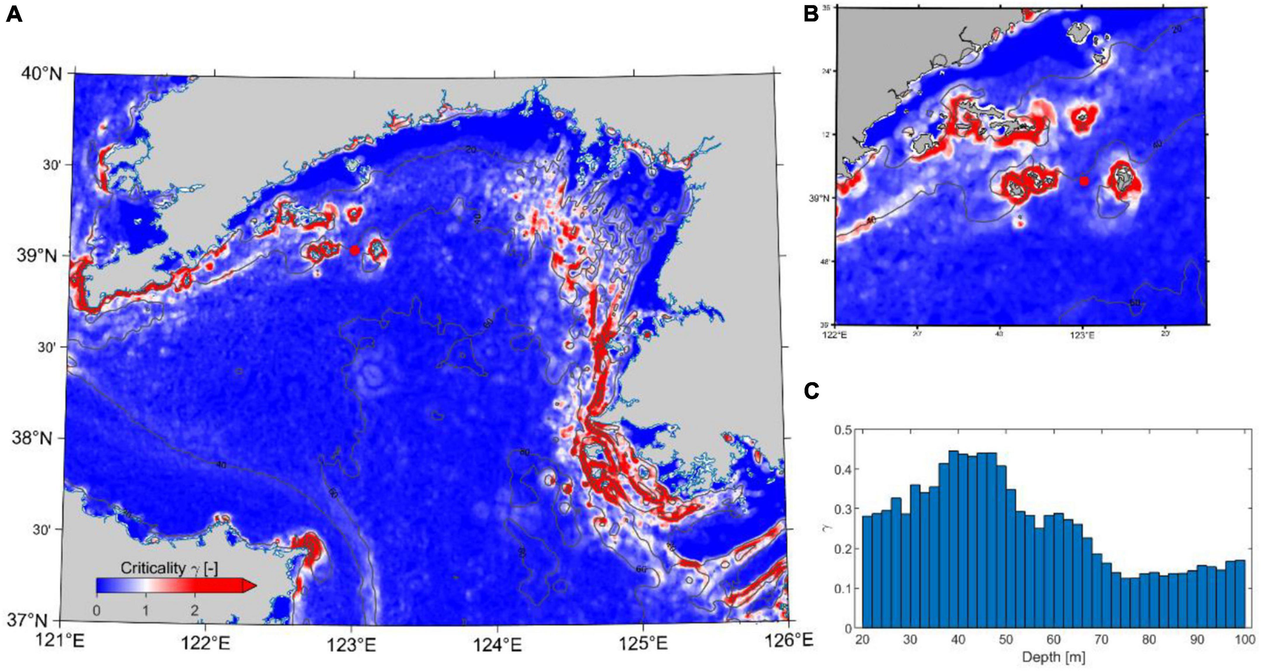
Figure 9. (A) Criticality of the topography on the northern Yellow Sea shelf estimated from the mean simulated buoyancy frequency near the bottom between July 26 and August 10. Solid lines represent the isobath contours of 20, 40, 60, and 80 m. (B) Detailed view of slope criticality near the mooring ADCP (red dot). (C) The depth-mean topographic criticality calculated for the northern Yellow Sea.

To visualize the internal tidal field, the vertical velocity fields computed from the difference between the baroclinic and barotropic M₂ model results are presented in Figures 10A,B with a 6-h time lag to represent the M₂ internal tide at 10 m depth. An opposite phase of the oscillation can be estimated from the striped patterns, which indicates propagation pathways. The internal tidal current is strong along the Korean coast with favorable generation conditions and abundant barotropic energy input (Figure 10). On the northern shelf near the Changshan islands, the internal tide propagates mainly along the tidal mixing front, passing the ADCP mooring. The horizontal wavelength and phase speed can also be estimated from the M₂ tidal period and the distance between each stripe, varying from 8.5 to 20 km and corresponding phase velocities between 0.19 and 0.45 m/s.

FIGURE 10

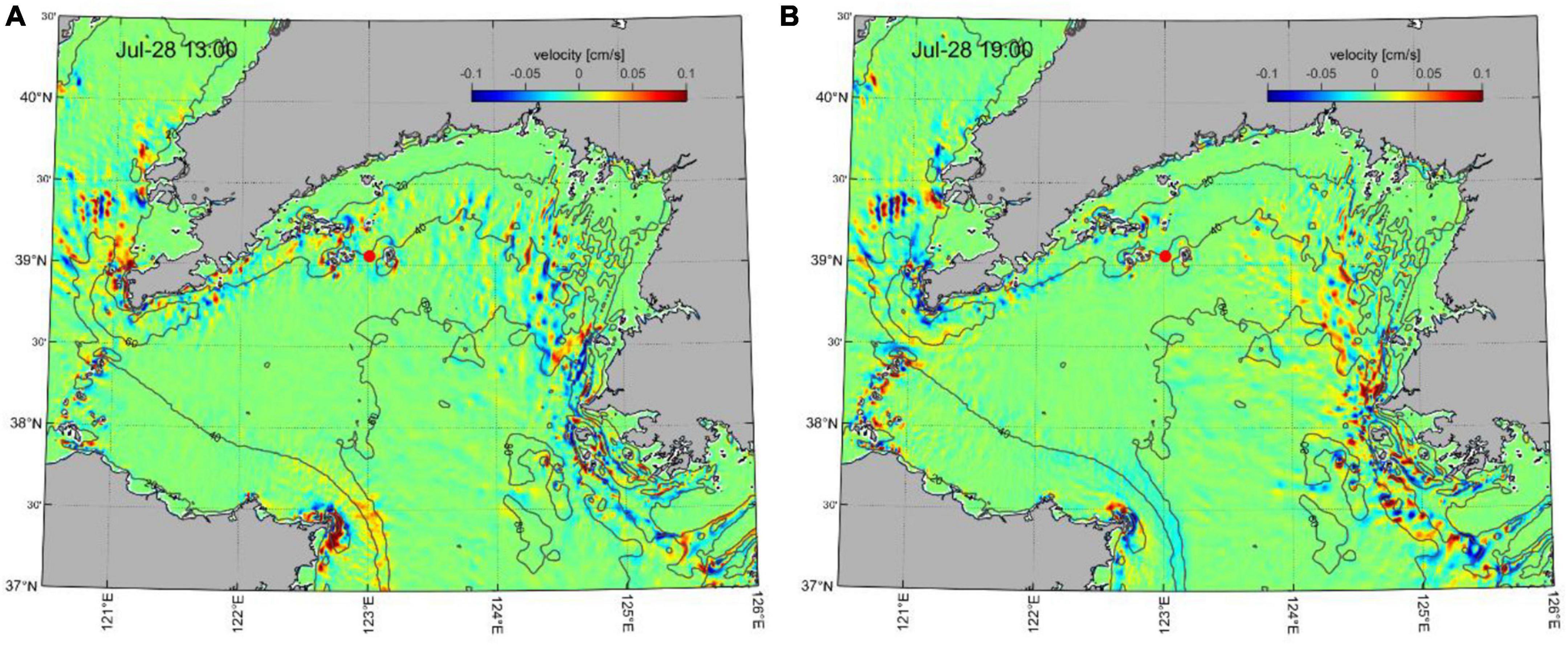
Figure 10. Simulated vertical velocity difference (cm/s) at 10 m depth for (A) 13:00 July 28 and (B) 19:00 July 28, computed from baroclinic and barotropic simulations forced with the M₂ tidal component at the boundary. Solid lines represent the isobath contours of 20, 40, 60, and 80 m. The red dot represents the ADCP mooring location.

The depth-integrated energy conversion rate (C) from the barotropic tide (BT) to the baroclinic tide (BC) is shown in Figure 11A. A positive energy conversion is occurring along the Korean coast, with typical conversion rates greater than 0.01 W/m², making it a significant source for the M₂ internal tide in the northern Yellow Sea (Figure 11A). The positive conversion rate is much weaker (between 0.005 and 0.01 W/m²) around the Changshan islands (Figure 11B), and with areas of negative conversion rates implying an energy transfer from BC to BT (<−0.01 W/m²). The depth-binned accumulated conversion rate (Figure 11C) shows that the positive conversion mainly occurs below the depth of 35 m and with a maximum of around 50–60 m.

FIGURE 11

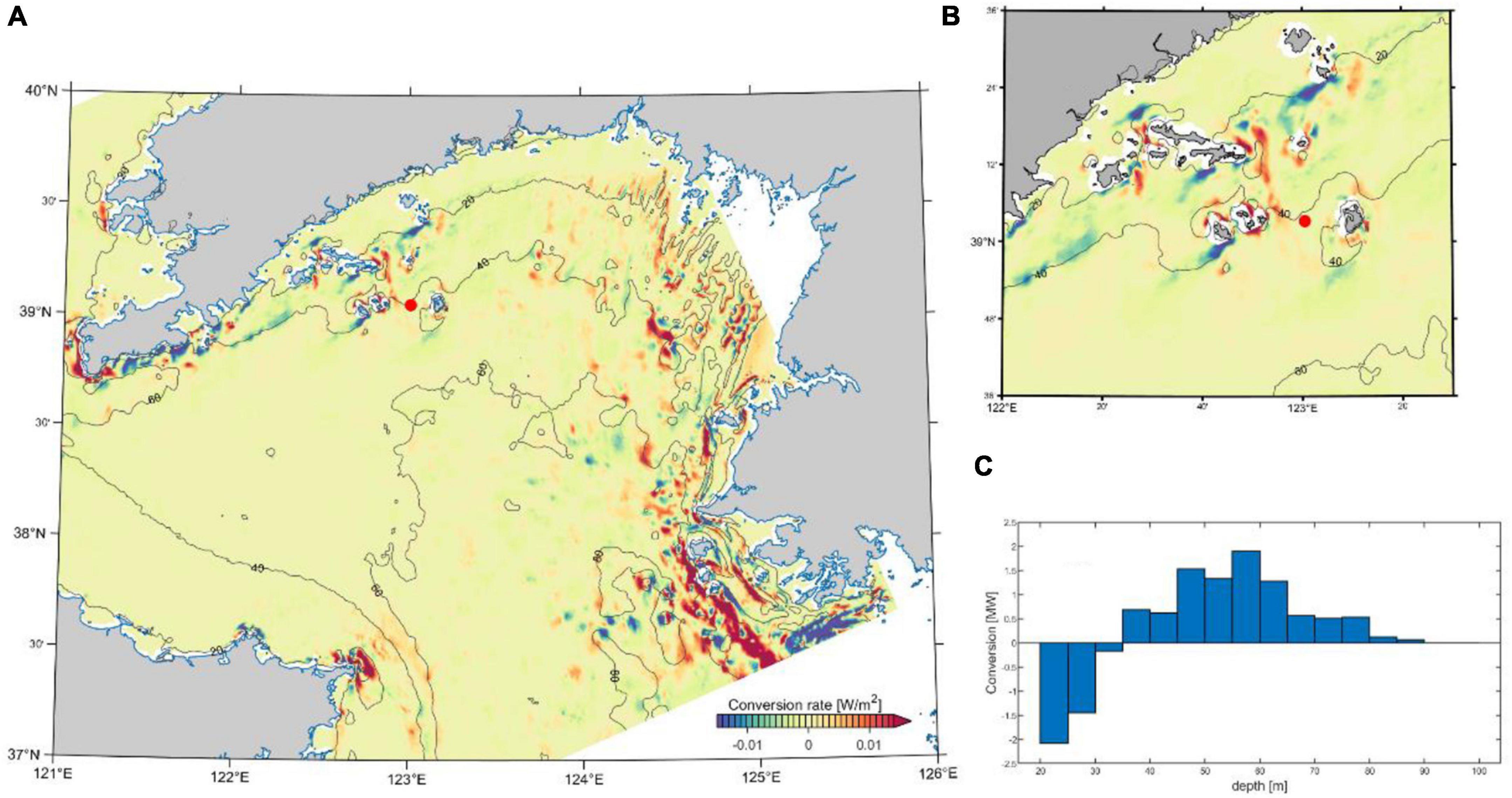
Figure 11. (A) Depth integrated and period averaged barotropic to baroclinic energy conversion (W/m²) in the northern Yellow Sea. Results were computed for the results from July 26 to August 10 in 2017. (B) The detailed conversion rate near the ADCP mooring site (red dot). (C) Mean conversion rate for binned depths within the domain in (A). Solid lines represent the isobath contour of 20, 40, 60, and 80 m.

The time-averaged and depth-integrated baroclinic energy flux F_bc is presented for the M₂ baroclinic simulation in Figure 12A. The M₂ internal tides generally have a diverse propagation pattern in the northern Yellow Sea. The F_bc originated from the Korean coast is strong and generally directed westward between 38.5 and 39.5°N. The maximum flux is approximately 45 W/m. When approaching the northern shelf of the Yellow Sea and near the 50 m isobaths, the baroclinic energy propagates northward onshore with gradually reduced energy. A zoomed pattern of the F_bc around the Changshan islands is shown in Figure 12B, and the baroclinic energy flux is much weaker around the islands, with a maximum value of ∼10 W/m. In the nearshore areas, almost no baroclinic energy is propagating as the water is nearly homogeneous.

FIGURE 12

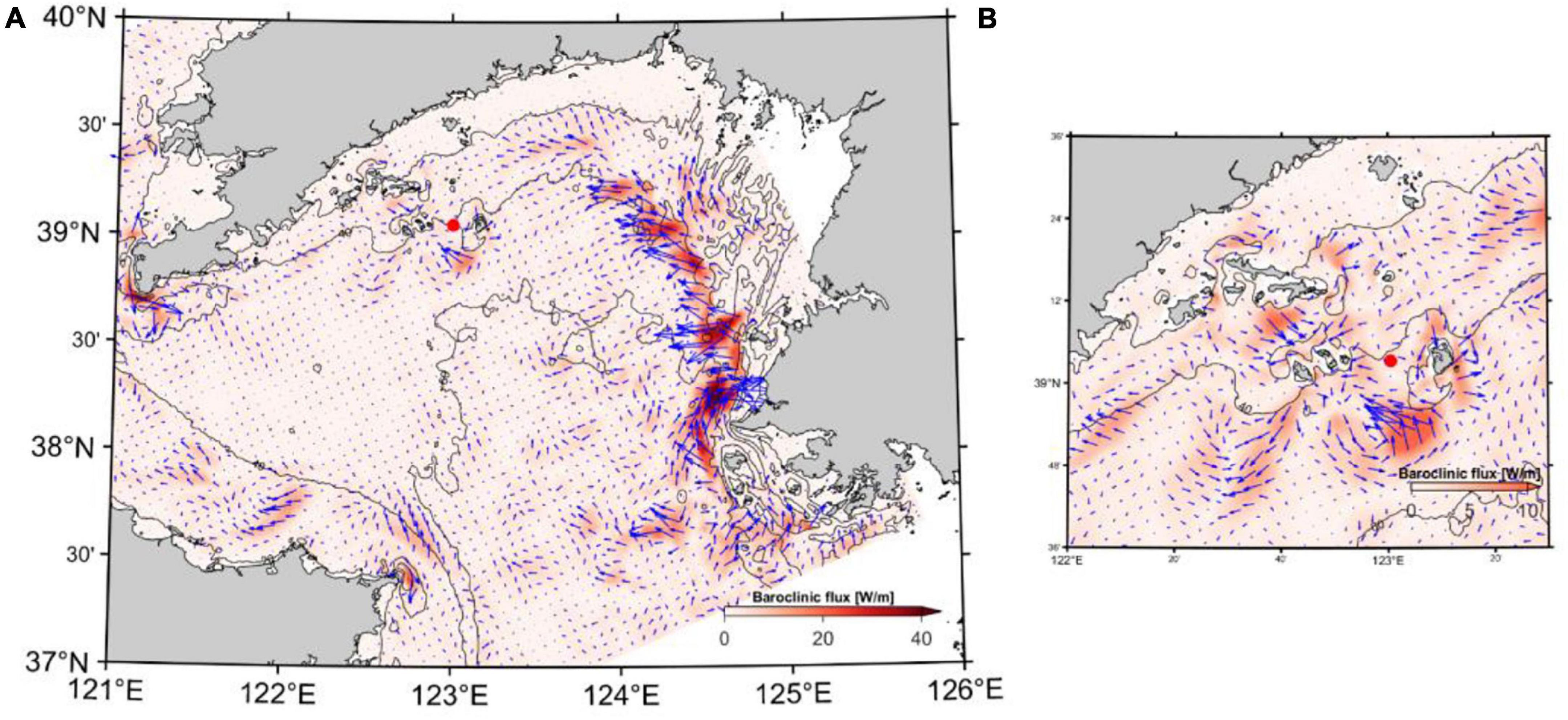
Figure 12. (A) The depth-integrated baroclinic energy flux (W/m) for the M2 semi-diurnal internal tide in the northern Yellow Sea averaged from July 26 to August 10, 2017. (B) Detailed view of the baroclinic energy flux near Changshan islands, with the ADCP mooring location shown as the red dot.

The time-averaged and depth-integrated coherent/incoherent baroclinic energy flux and the corresponding flux divergence derived from the M₂ baroclinic model results are presented for Changshan islands and the adjacent seas in Figure 13. The locations with high values of the coherent baroclinic energy flux and divergence (Figure 13A) coincide with the locations where the barotropic energy converts into baroclinic energy (Figure 11). Coherent baroclinic energy flux radiates away from the generation sites around the island. The M₂ internal tide mainly propagates westward, and the energy flux damps quickly after a few kilometers. The coherent M₂ baroclinic energy flux divergence is mostly negative around the Changshan islands, indicating a net loss of coherent energy within the domain. The incoherent baroclinic energy flux is almost an order of magnitude smaller than the coherent ones (Figure 13B), implying the internal tide generated at remote locations is weak in this region.

FIGURE 13

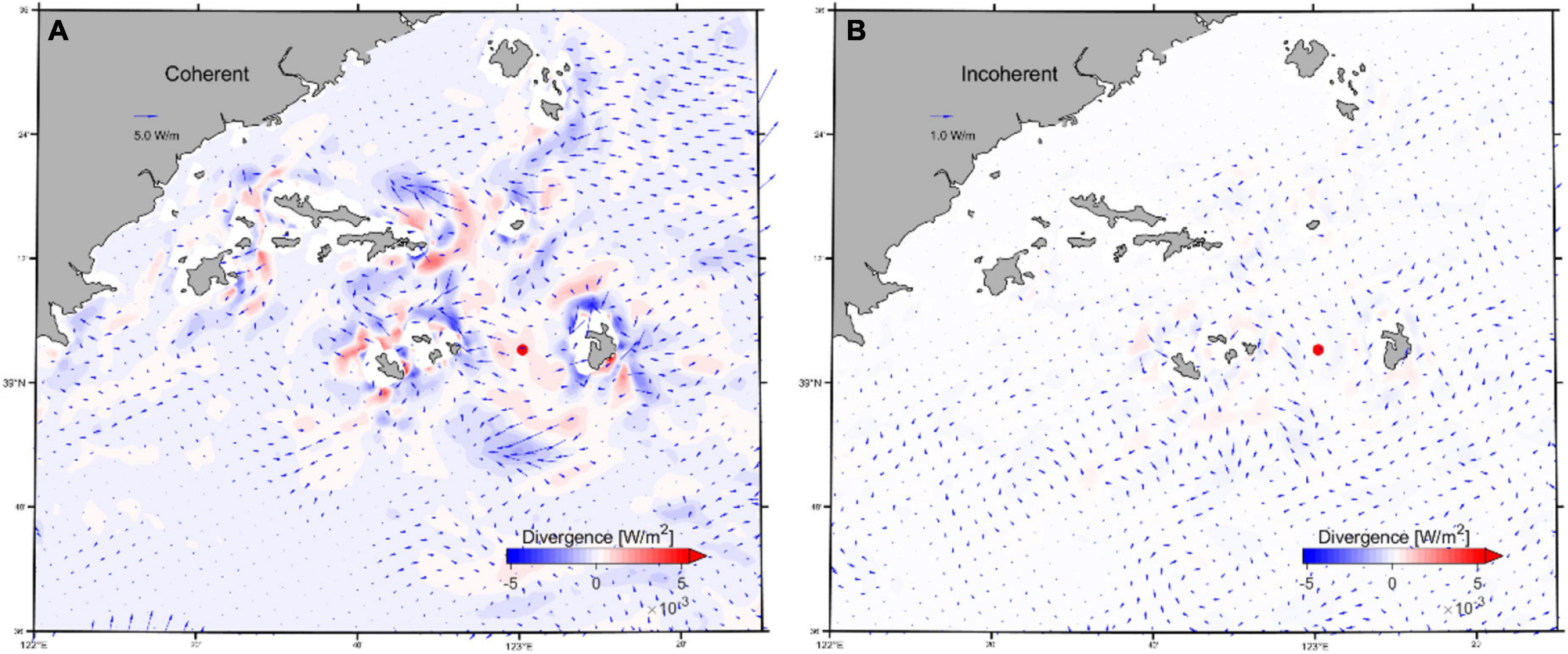
Figure 13. (A) The coherent baroclinic energy flux (F_coh, arrow W/m) and the flux divergence (∇_H⋅F_coh, W/m²) derived for 10 tidal cycles for the M₂ internal tide around the Changshan islands. (B) The incoherent baroclinic flux (F_incoh, arrow W/m) and flux divergence (∇_H⋅F_incoh, W/m²) for the same region. ADCP mooring location is represented as red dot.

Discussion

Model Performance

Numerical models are suitable to study and describe the dynamics of internal tide in various regions of the world (Kang and Fringer, 2012; Nash et al., 2012; Masunaga et al., 2017; Liu et al., 2019; Davis et al., 2020). As the horizontal scale of the internal tide in the Yellow Sea is much larger than the regional depth, a hydrostatic model is sufficient to describe the features of the phenomena. The hydrodynamic model employed in this study has previously been applied to describe the hydrodynamics in the northern Yellow Sea by Lin et al. (2019) as well as in numerous applications worldwide¹. The model results from the Yellow Sea were validated against current and water temperature observations and did reproduce the summertime total current field and thermohaline structure reasonably well (Lin et al., 2019).

In the present study, current observations from the summer of 2017 were compared to model results focusing on the baroclinic current features. The total horizontal current at different layers calculated by the current model agrees well with the observation results. The model results do reasonably reproduce the current magnitude and direction at all depths (the averaged RMS error is 0.12 m/s). The barotropic tide is dominant in this region, but the vertical current structure with a stronger flow speed toward the bottom is apparent in both the observation and simulation (Figure 2), demonstrating a robust baroclinic signal at the observation site. This baroclinic signal is a semi-diurnal mode-1 wave (Figure 4). With the barotropic component removed, the model results resemble a temporal-spatial baroclinic velocity pattern comparable to the observation. The barotropic and baroclinic tidal ellipses of the M₂ component also compare well between the observation and simulation results (Figure 5), indicating the dynamics of the internal tides are reproduced by the model. The spectral analysis results (Figure 6) illustrate that the M₂ internal tide is dominant in the entire water column but with a noisier pattern in the observations. The simulated baroclinic spectrum demonstrates a similar energy distribution concentrated around the diurnal and semi-diurnal frequencies. The discrepancy between the observation and simulation results is probably due to the inaccuracy in the background model stratification and smoothed bathymetry related to challenges in modeling turbulent mixing and potentially inaccurate depth data for this region. Also, the 1 km grid size will somewhat smooth the model results compared to the ADCP data.

Nevertheless, the comparison of the model results and observation shows that the hydrodynamic model is capable of reproducing the internal tides in the northern Yellow Sea.

Generation and Propagation of the Internal Tide in the Northern Yellow Sea

The focus of this study is to investigate the generation and propagation mechanism of the internal tides in the northern Yellow Sea. The current system in the Yellow Sea is dominated by the barotropic tides (Ichikawa and Beardsley, 2002; Xia et al., 2006; Hwang et al., 2014; Lin et al., 2019), with the main being the M₂ component for which the current amplitude is ∼0.5 m/s on the northern shelf (Lin et al., 2019). We concentrate on the M₂ internal tide since it is the dominating baroclinic component and can propagate with respect to the frequency restriction. Liu et al. (2019) have studied the seasonal and spatial distribution of the M₂ internal tides in the entire Yellow Sea and concluded with multiple sources and a complex interference internal tidal field in the summer. They focused on the southern Yellow Sea where the stratification is well established with the year-round buoyancy flux input from the Yangtze River estuary. In the northern Yellow Sea, the water depth is relatively shallow (<80 m), and the most intensive stratification is found at the seasonal thermocline above the YSBCW, where the buoyancy frequency can be around 2 × 10^–3 s^–1 (Lin et al., 2019), allowing the propagation of high-frequency internal waves. In the tidal mixing front along the shelf break, a typical depth-averaged buoyancy frequency is about 4.3 × 10^–4 s^–1, satisfying the generation and propagation of the semi-diurnal internal tides with a frequency of about 2.2 × 10^–5 s^–1 (Figure 9). Hence, the M₂ internal tide in the northern Yellow Sea is mainly generated from the rugged topography within the tidal mixing front along the coast.

The various internal tidal wavelengths and the interference patterns computed from the M₂ internal tidal current field at 10 m depth (Figure 10) are consistent with previous studies (Liu et al., 2019). The relatively strong internal tidal signal appears to be within the tidal mixing front, coinciding with the generation pattern presented in Figure 9. A high BT-BC energy conversion (Figure 11A) occurs along the Korean coast where the tidal current is strong and supplies abundant kinetic energy (Lin et al., 2019). The negative conversion around this region may probably be caused by a remotely generated internal tide being superposed with locally generated ones, which does not refer to energy conversion from baroclinic tide to barotropic tide (Kang and Fringer, 2012; Masunaga et al., 2017). The detailed conversion pattern around the Changshan islands (Figure 11B) illustrates that the positive conversion here can be the source of the internal tidal signal captured at the current meter mooring location. The depth accumulated BT-BC conversion for the presented area (Figure 11C) implies that most internal tides inshore of 35 m isobath have been propagating from the deeper part, probably generated at the tidal mixing front nearby.

The depth-integrated and period-averaged baroclinic energy flux (Figure 12A) demonstrates a specific pattern of the internal tidal propagation for the simulation period. Because of the shallow bathymetry in the Yellow Sea (average depth of 44 m), the total baroclinic energy is non-comparable to that of the deep seas such as the South China Sea or Monterey Bay (Jan et al., 2008; Kang and Fringer, 2012). From the results of Liu et al. (2019), the most active region for baroclinic energy propagation is near the Yangtze River, with a typical energy flux of more than 100 W/m. In the northern Yellow Sea, baroclinic energy from the internal tide is mainly propagating westward from the Korean coast between the latitude of 38.5∼39.5°N. The maximum magnitude is around 45 W/m, and this is damped rapidly. The baroclinic energy flux is much weaker near the Changshan islands (Figure 12B), mainly due to less barotropic kinetic energy available. The relatively strong baroclinic energy flux in this region originates between the 40∼50 m isobaths near the islands, suggesting that the M₂ internal tidal signal captured by the ADCP is probably generated locally. This can also be confirmed from the spatial pattern of the coherent and incoherent baroclinic energy flux (Figures 13A,B). Coherent energy flux is dominant on the northern shelf, implying the baroclinic energy of the internal tide is mainly generated from local barotropic tides (Figure 13A). The coherent flux generally becomes stronger when propagating away from the islands and is damped toward the islands. The complicated and shallow topography around the Changshan islands makes the local generated internal tide a short-lived phenomenon limited to the neighboring area. The incoherent energy flux (Figure 13B) is about an order of magnitude smaller than the coherent energy flux, which is consistent with the results from the current observations from the ADCP (Figure 7).

From the perspective of the entire Yellow Sea, the internal tidal induced mixing only accounts for a small amount (∼0.8%) of the total tidal mixing. However, it can be important when discussing the enhanced turbulent mixing near the pycnoclines (Liu et al., 2019). When it comes to the northern shelf of the Yellow Sea where most regions either consist of homogeneous water or are located in the mixing front, the impact on currents is more prominent. The barotropic tide is most important for local water mass transportation (Lin et al., 2019), but in areas around the Changshan islands where locally generated internal tides are strong, the barotropic current will be modified by the internal tide. Typically, the internal tide will have a first mode or two-layer structure with the flow in the direction of the barotropic tide in the lower layer and the opposite direction in the upper layer (Figure 8). The interface of this two-layer structure is usually at a depth of approximately 25 m (Figure 4) and may vary with the background stratification caused by the barotropic advection and spring-neap tidal cycles. Generally, the internal tidal current is stronger at the bottom (Figures 8C,D) and at about 30% of the speed for the barotropic M₂ component. This superposed barotropic and baroclinic current may strengthen the bottom material transport within the northern shelf horizontally during each tidal oscillation. The vertical shear imposed by the internal tide may also enhance the turbulent mixing across the water column in the tidal mixing front. Thus, promoting the material exchange in this aquaculture region on the northern shelf of the Yellow Sea.

Conclusion

The barotropic tide is important for the currents in the Yellow Sea and dominates the dynamics on the northern shelf. Our study using data from a current meter mooring and a regional current model, shows that also the semi-diurnal internal tide can be important in the northern Yellow Sea. The results indicate that:

• A mode-1, semi-diurnal internal tide is generated in the tidal mixing front of the northern shelf of the Yellow Sea.

• The current of the internal tide is in the same direction as the barotropic tide in the lower layer, adding to the total current toward the bottom.

• The internal tide is mainly generated locally and with a limited regional propagation.

• The shelf break areas toward the Korean coast are the most prominent locations for generation of the internal tide.

Data Availability Statement

The raw data supporting the conclusions of this article will be made available by the authors, without undue reservation.

Author Contributions

FL: manuscript writing and revision, model setup and run, data analysis, and data collection. LA: manuscript writing and revision and data analysis. HW: manuscript revision and data collection. All authors contributed to the article and approved the submitted version.

Funding

This research was jointly funded by the Sino-EU Cooperative Research on Ecosystem-based Spatial Planning for Aquaculture (2017YFE0112600) and the Central Public-interest Scientific Institution Basal Research Fund, CAFS (NO. 2020TD50). This research was also supported by the Research Council of Norway (249056/H30), and the Environment and Aquaculture Governance project (MFA, CHN 2152).

Conflict of Interest

The authors declare that the research was conducted in the absence of any commercial or financial relationships that could be construed as a potential conflict of interest.

Publisher’s Note

All claims expressed in this article are solely those of the authors and do not necessarily represent those of their affiliated organizations, or those of the publisher, the editors and the reviewers. Any product that may be evaluated in this article, or claim that may be made by its manufacturer, is not guaranteed or endorsed by the publisher.

Acknowledgments

We appreciate the support from Tianjin University and the Sea Ranching Research Center of Zoneco Co., Ltd., for their help in making observations. We also thank the European Center for Medium-Range Weather Forecasts for the atmospheric data, the international team of GEBCO for bathymetry data and NOPP for HYCOM data.

Footnotes

1. ^ www.myroms.org

References

Becker, J. J., Sandwell, D. T., Smith, W. H. F., Braud, J., Binder, B., Depner, J., et al. (2009). Global Bathymetry and Elevation Data at 30 Arc Seconds Resolution: SRTM30_PLUS. Mar. Geod. 32, 355–371. doi: 10.1080/01490410903297766

CrossRef Full Text | Google Scholar

Cacchione, D. A., Pratson, L. F., and Ogston, A. S. (2002). The Shaping of Continental Slopes by Internal Tides. Science 296, 724–727. doi: 10.1126/science.1069803

PubMed Abstract | CrossRef Full Text | Google Scholar

Carter, G., Fringer, O., and Zaron, E. (2012). Regional Models of Internal Tides. Oceanography 25, 56–65. doi: 10.5670/oceanog.2012.42

CrossRef Full Text | Google Scholar

Davis, K. A., Arthur, R. S., Reid, E. C., Rogers, J. S., Fringer, O. B., DeCarlo, T. M., et al. (2020). Fate of internal waves on a shallow shelf. J. Geophys. Res. Oceans 125. doi: 10.1029/2019jc015377

CrossRef Full Text | Google Scholar

Dee, D. P., Uppala, S. M., Simmons, A. J., Berrisford, P., Poli, P., Kobayashi, S., et al. (2011). The ERA−Interim reanalysis: configuration and performance of the data assimilation system. Q. J. Roy. Meteor. Soc. 137, 553–597. doi: 10.1002/qj.828

CrossRef Full Text | Google Scholar

Egbert, G. D., and Erofeeva, S. Y. (2002). Efficient Inverse Modeling of Barotropic Ocean Tides. J. Atmos. Ocean Tech. 19, 183–204. doi: 10.1175/1520-04262002019<0183:eimobo<2.0.co;2

CrossRef Full Text | Google Scholar

Egbert, G. D., and Ray, R. D. (2001). Estimates of M2 tidal energy dissipation from TOPEX/Poseidon altimeter data. J. Geophys. Res. Oceans 106, 22475–22502. doi: 10.1029/2000jc000699

CrossRef Full Text | Google Scholar

Fairall, C. W., Bradley, E. F., Rogers, D. P., Edson, J. B., and Young, G. S. (1996). Bulk parameterization of air−sea fluxes for Tropical Ocean−Global Atmosphere Coupled−Ocean Atmosphere Response Experiment. J. Geophys. Res. Oceans 101:3764. doi: 10.1029/95jc03205

CrossRef Full Text | Google Scholar

Guo, S., and Hu, T. (2010). Simulating the effects of the internal tide in the Yellow Sea on acoustic propagation. J. Harb. Eng. Univ. 31, 967–974.

Google Scholar

Haidvogel, D. B., Arango, H., Budgell, W. P., Cornuelle, B. D., Curchitser, E., Lorenzo, E. D., et al. (2008). Ocean forecasting in terrain-following coordinates: Formulation and skill assessment of the Regional Ocean Modeling System. J. Comput. Phys. 227:3624. doi: 10.1016/j.jcp.2007.06.016

CrossRef Full Text | Google Scholar

Hwang, J. H., Van, S. P., Choi, B.-J., Chang, Y. S., and Kim, Y. H. (2014). The physical processes in the Yellow Sea. Ocean Coast Manage 102:457. doi: 10.1016/j.ocecoaman.2014.03.026

CrossRef Full Text | Google Scholar

Ichikawa, H., and Beardsley, R. C. (2002). The Current System in the Yellow and East China Seas. J. Oceanogr. 58, 77–92.

Google Scholar

Jan, S., Lien, R.-C., and Ting, C.-H. (2008). Numerical study of baroclinic tides in Luzon Strait. J. Oceanogr. 64, 789. doi: 10.1007/s10872-008-0066-5

CrossRef Full Text | Google Scholar

Kang, D., and Fringer, O. (2012). Energetics of Barotropic and Baroclinic Tides in the Monterey Bay Area. J. Phys. Oceanogr. 42, 272–290. doi: 10.1175/jpo-d-11-039.1

CrossRef Full Text | Google Scholar

Kumar, N., Suanda, S. H., Colosi, J. A., Haas, K., Lorenzo, E. D., Miller, A. J., et al. (2019). Coastal Semi-diurnal Internal Tidal Incoherence in the Santa Maria Basin, California: Observations and Model Simulations. J. Geophys. Res. Oceans 124, 5158–5179. doi: 10.1029/2018jc014891

CrossRef Full Text | Google Scholar

Lee, J. H., Lozovatsky, I., Jang, S., Jang, C. J., Hong, C. S., and Fernando, H. J. S. (2006). Episodes of nonlinear internal waves in the northern East China Sea. Geophys. Res. Lett. 33:27136. doi: 10.1029/2006gl027136

CrossRef Full Text | Google Scholar

Li, B., Wei, Z., Wang, X., Fu, Y., Fu, Q., Li, J., et al. (2020). Variability of coherent and incoherent features of internal tides in the north South China Sea. Sci. Rep. 10:12904. doi: 10.1038/s41598-020-68359-7

PubMed Abstract | CrossRef Full Text | Google Scholar

Lin, F., Asplin, L., Budgell, P., Wei, H., and Fang, J. (2019). Currents on the northern shelf of the Yellow Sea. Regional. Stud. Mar. Sci. 32:100821. doi: 10.1016/j.rsma.2019.100821

CrossRef Full Text | Google Scholar

Liu, K., Sun, J., Guo, C., Yang, Y., Yu, W., and Wei, Z. (2019). Seasonal and Spatial Variations of the M2 Internal Tide in the Yellow Sea. J. Geophys. Res. 124, 1115–1138. doi: 10.1029/2018JC014819

CrossRef Full Text | Google Scholar

Liu, Z., Wei, H., Lozovatsky, I. D., and Fernando, H. J. S. (2009). Late summer stratification, internal waves, and turbulence in the Yellow Sea. J. Mar. Syst. 77, 459–472. doi: 10.1016/j.jmarsys.2008.11.001

CrossRef Full Text | Google Scholar

Masunaga, E., Fringer, O. B., Kitade, Y., Yamazaki, H., and Gallager, S. M. (2017). Dynamics and energetics of trapped diurnal internal Kelvin waves around a mid-latitude island. J. Phys. Oceanogr. 47, 2479–2498. doi: 10.1175/jpo-d-16-0167.1

CrossRef Full Text | Google Scholar

Nash, J., Shroyer, E., Kelly, S., Inall, M., Duda, T., Levine, M., et al. (2012). Are Any Coastal Internal Tides Predictable? Oceanography 25, 80–95. doi: 10.5670/oceanog.2012.44

CrossRef Full Text | Google Scholar

Shang, X., Liu, Q., Xie, X., Chen, G., and Chen, R. (2015). Characteristics and seasonal variability of internal tides in the southern South China Sea. Deep Sea Res. Part Oceanogr. Res. Pap. 98, 43–52. doi: 10.1016/j.dsr.2014.12.005

CrossRef Full Text | Google Scholar

Shchepetkin, A. F., and McWilliams, J. C. (2005). The regional oceanic modeling system (ROMS): a split-explicit, free-surface, topography-following-coordinate oceanic model. Ocean Model 9, 347–404. doi: 10.1016/j.ocemod.2004.08.002

CrossRef Full Text | Google Scholar

Tana, Fang, Y., Liu, B., Sun, S., and Wang, H. (2017). Dramatic weakening of the ear-shaped thermal front in the Yellow Sea during 1950s–1990s. Acta Oceanol. Sin. 36, 51–56. doi: 10.1007/s13131-016-0885-y

CrossRef Full Text | Google Scholar

Thorpe, S. A. (1998). Physical Processes in Lakes and Oceans. Coast Estuar. Stud. 1998, 441–460. doi: 10.1029/ce054p0441

CrossRef Full Text | Google Scholar

Wang, Z., Li, Q., Wang, C., Qi, F., Duan, H., and Xu, J. (2020). Observations of internal tides off the coast of Shandong Peninsula. China. Estuar. Coast Shelf Sci. 245:106944. doi: 10.1016/j.ecss.2020.106944

CrossRef Full Text | Google Scholar

Warner, J. C., Sherwood, C. R., Arango, H. G., and Signell, R. P. (2005). Performance of four turbulence closure models implemented using a generic length scale method. Ocean Model 8, 81–113. doi: 10.1016/j.ocemod.2003.12.003

CrossRef Full Text | Google Scholar

Wei, H., Yuan, C., Lu, Y., Zhang, Z., and Luo, X. (2013). Forcing mechanisms of heat content variations in the Yellow Sea. J. Geophys. Res. Oceans 118, 4504–4513. doi: 10.1002/jgrc.20326

CrossRef Full Text | Google Scholar

Xia, C., Qiao, F., Yang, Y., Ma, J., and Yuan, Y. (2006). Three−dimensional structure of the summertime circulation in the Yellow Sea from a wave−tide−circulation coupled model. J. Geophys. Res. Oceans 111:297.

Google Scholar

Yan, T., Qi, Y., Jing, Z., and Cai, S. (2020). Seasonal and spatial features of barotropic and baroclinic tides in the northwestern South China Sea. J. Geophys. Res. 125:e2018JC014860. doi: 10.1029/2018JC014860

CrossRef Full Text | Google Scholar

Zhu, J., Shi, J., Guo, X., Gao, H., and Yao, X. (2017). Air-sea heat flux control on the Yellow Sea Cold Water Mass intensity and implications for its prediction. Cont. Shelf Res. 152, 14–26. doi: 10.1016/j.csr.2017.10.006

CrossRef Full Text | Google Scholar