
94% of researchers rate our articles as excellent or good
Learn more about the work of our research integrity team to safeguard the quality of each article we publish.
Find out more
ORIGINAL RESEARCH article
Front. Mar. Sci., 06 January 2022
Sec. Physical Oceanography
Volume 8 - 2021 | https://doi.org/10.3389/fmars.2021.794156
 Ruijie Ye1,2
 Xiaodong Shang3Wei Zhao2,4
 Chun Zhou2,4*
 Qingxuan Yang2,4
 Zichen Tian2Yongfeng Qi3Changrong Liang3
 Xiaodong Huang2,4
 Zhiwei Zhang2,4Shoude Guan2,4
 Jiwei Tian2,4
Turbulent mixing above rough topography is crucial for the vertical motions of deep water and the closure of the meridional overturning circulation. Related to prominent topographic features, turbulent mixing not only exhibits a bottom-intensified vertical structure but also displays substantial lateral variation. How turbulent mixing varies in the upslope direction and its impact on the upwelling of deep water over sloping topography remains poorly understood. In this study, the notable multihump structure of the bottom-intensified turbulent diffusivity in the upslope direction of a seamount in the South China Sea (SCS) is revealed by full-depth fine-resolution microstructure and hydrographic profiles. Numerical experiments indicate that multihump bottom-intensified turbulent mixing around a seamount could lead to multiple cells of locally strengthened circulations consisting of upwelling (downwelling) motions in (above) the bottom boundary layer (BBL) that are induced by bottom convergence (divergence) of the turbulent buoyancy flux. Accompanied by cyclonic (anticyclonic) flow, a three-dimensional spiral circulation manifests around the seamount topography. These findings regarding the turbulent mixing and three-dimensional circulation around a deep seamount provide support for the further interpretation of the abyssal meridional overturning circulation.
Turbulent mixing in the deep ocean plays a fundamental role not only in transforming bottom dense water into lighter water and maintaining the deep stratification (Munk, 1966; Munk and Wunsch, 1998; Wunsch and Ferrari, 2004) but also in shaping the deep ocean overturning circulation (Munk and Wunsch, 1998; Wunsch and Ferrari, 2004; Stewart et al., 2012; de Lavergne et al., 2016). Accordingly, studies conducted over many years have revealed that, due to interactions between rough topography and abyssal internal tides, mesoscale or submesoscale processes, turbulent mixing is enhanced by 2–3 orders of magnitude toward the ocean bottom (e.g., Toole et al., 1994, 1997; Polzin et al., 1997; Ledwell et al., 2000; Naveira Garabato et al., 2004; Tian et al., 2009; Yang et al., 2016; Ruan et al., 2017).
However, contrary to the previous conjecture that deepwater upwells to the upper layers as a result of a diabatic transformation induced by enhanced mixing in the upper ocean (Munk, 1966; Munk and Wunsch, 1998), the bottom intensification of turbulent mixing indicates that the turbulent buoyancy flux diverges in the stratified mixing layer (SML) overlying the ocean bottom, suggesting the diapycnal downwelling motions of deep water (Polzin et al., 1997; Ledwell et al., 2000; St. Laurent et al., 2001). This conundrum can be explained theoretically by considering the bottom boundary layer (BBL) around rough topography (Ferrari et al., 2016; McDougall and Ferrari, 2017). Whereas turbulent mixing shows bottom intensification to satisfy the no-flux boundary condition, the turbulent buoyancy flux converges in the BBL, inducing diapycnal upwelling motions there. This highlights the vital role of diapycnal upwelling motions along with the BBL over sloping topography in closing the meridional overturning circulation (Holmes et al., 2018; Drake et al., 2020).
Seamounts are ubiquitous topographic features found throughout the global ocean, with over 100,000 seamounts estimated worldwide with heights exceeding 1 km (Kitchingman et al., 2007; Wessel et al., 2010). Seamounts have been characterized as ocean stirring rods with rough flanks (Perfect et al., 2020), thereby serving as loci where some large-scale current and barotropic tides cascade their energy into smaller-scale turbulent dissipation (Garrett, 2003) and induce bottom-intensified turbulent mixing (Toole et al., 1997; Lavelle et al., 2004; Carter et al., 2006). Accordingly, dipolar diapycnal flow is expected to occur within the boundary layer around seamounts with upwelling motions in the BBL and downwelling motions in the SML (e.g., McDougall, 1989; Ferrari et al., 2016; McDougall and Ferrari, 2017; Holmes and McDougall, 2020). However, these studies have not fully explored the impact of upslope variations in the peak turbulent mixing intensity over sloping bottom topography.
Nevertheless, increasing observational evidence suggests that when the ocean bottom topographic roughness is non-uniformly distributed, bottom-intensified turbulent mixing could manifest as multiple hotspots in the upslope direction of sloping bottom topography (Lueck and Mudge, 1997; Polzin et al., 1997; Toole et al., 1997; Naveira Garabato et al., 2004; Nash et al., 2007; Wain and Rehmann, 2010; Kunze et al., 2012). To better understand the role of turbulent mixing in the deep ocean overturning circulation, the effects of the lateral (i.e., upslope) structure of bottom-intensified turbulent mixing on the circulation above sloping topography need to be further explored. In this study, based on in situ observations around a seamount in the South China Sea (SCS), where enhanced turbulent mixing has been revealed due to energetic multiscale dynamic processes (Tian et al., 2009), the spatial distribution of turbulent mixing and the flow structure around the seamount is revealed. Moreover, a set of numerical experiments configured with different spatial distributions of turbulent mixing are carried out over a seamount to explore the modulation of the flow structure around the seamount with multihump turbulent mixing, indicating multiple peaks in the intensity of turbulent mixing in the upslope direction.
Shipboard observations were conducted on a steep seamount located in the central SCS (Figure 1A). With an ocean bottom depth of ∼4,000 m and a diameter of ∼40 km, the seamount rises to ∼200 m below the surface. Three full-depth casts of a free-fall vertical microstructure profiler (VMP, Rockland Scientific International Inc.) were launched to acquire profiling measurements of the microscale velocity shear and temperature of the northern slope of the seamount (Figure 1B). The shallowest profile (P1) was recorded by a tethered free-falling instrument (VMP-250), whereas the other two profiles (P2 and P3) were recorded by a VMP-Expendable (VMP-X) device. Upon touching the seafloor, VMP-X drops a non-recoverable sensor package equipped with two shear probes and one thermistor and returns to the surface with records of the microscale velocity shear and temperature of the entire water column, especially the BBL (Shang X. et al., 2017).
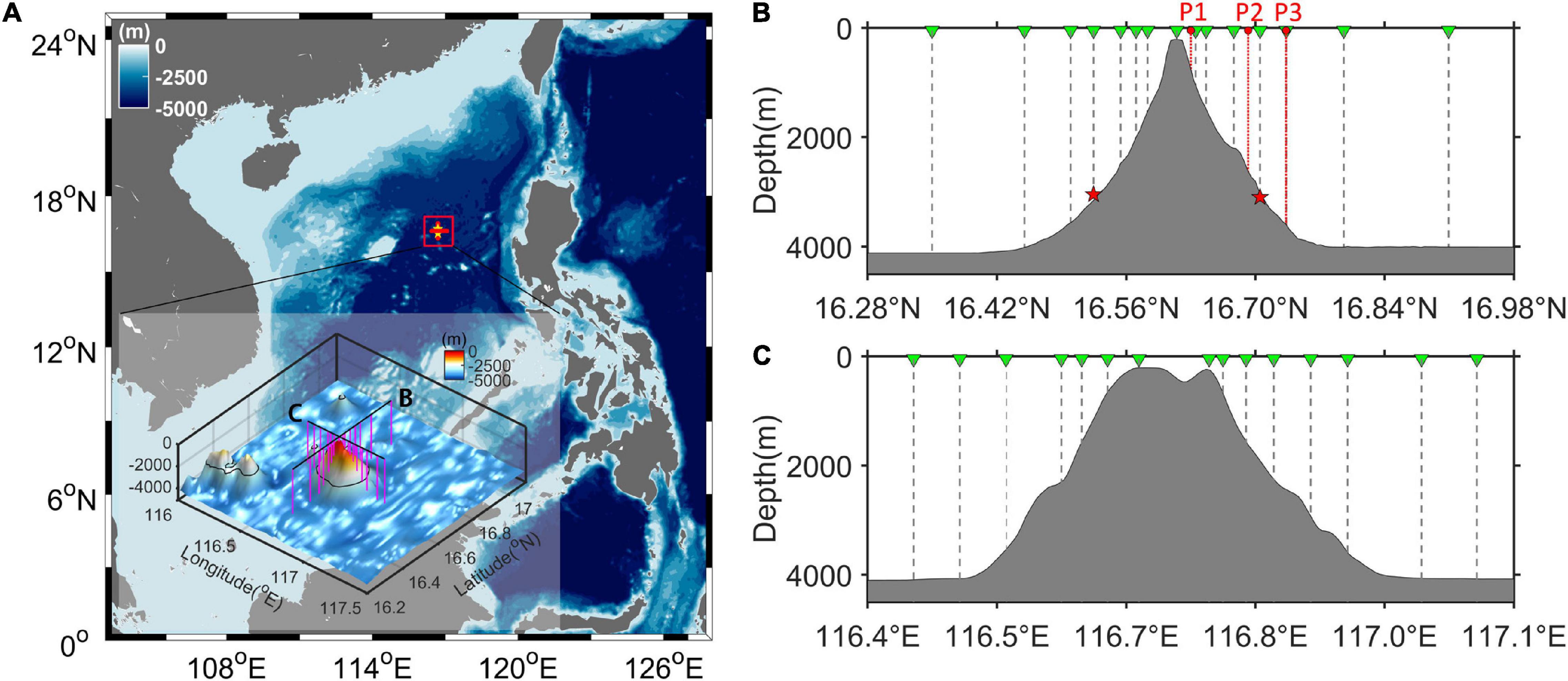
Figure 1. (A) Bottom topography of the SCS based on Smith and Sandwell (1997) with a resolution of 1’. The enlarged map presents the cross-shaped hydrographic section at the seamount. The magenta vertical lines indicate CTD profiles. (B,C) Meridional and zonal sections of the seamount, respectively. The green triangles indicate the CTD profiles, and the red circles indicate the VMP profiles. The red stars display the deep mooring locations.
The turbulent kinetic energy (TKE) dissipation rate (ε) was calculated by fitting the Nasmyth spectrum to the measured shear spectra (Shay and Gregg, 1986; Peters et al., 1988). The turbulent diffusivity was estimated using Osborn’s relation (Osborn, 1980) as κρ = Γε/N2, where ε is the TKE dissipation rate estimated from VMP measurements, N2 is the buoyancy frequency calculated from simultaneous conductivity–temperature–depth (CTD) casts, and Γ is the mixing efficiency. For simplicity, a canonical value of 0.2 for the mixing efficiency Γ was adopted (Polzin et al., 1997; Lavelle et al., 2004; Waterhouse et al., 2014; Gregg et al., 2018). Considering the possible contamination by surface waves and ship wakes, the top 10 m of each turbulent mixing dissipation rate profile was discarded in this study.
Furthermore, two orthogonal transects of hydrographic measurements were conducted over the seamount with a horizontal resolution of ∼2 km (Figures 1B,C). The instruments involved were a shipboard SBE 911plus CTD sensor with a sampling rate of 24 Hz and a Teledyne RD Instruments 300 kHz Lowered Acoustic Doppler Current Profiler (LADCP) with a vertical bin size of 8 m. The CTD/LADCP instruments were lowered at a rate of about 0.8 m s–1. The buoyancy frequency and velocity shear mentioned below are finally calculated over 10 m intervals. An acoustic altimeter was mounted on the CTD rosette to ensure that the CTD descended to within 10 m above the bottom. In addition, two short-term deep moorings configured with current meters and CTD sensors were deployed from June 23, 2017, to June 25, 2017, and located on the northern and southern slopes of the seamount to monitor the currents around the seamount.
A series of numerical experiments are carried out using the MIT general circulation model (MITgcm) (Marshall et al., 1997a,b) to explore the mechanism by which the circulation around a seamount is modulated by inhomogeneously distributed turbulent mixing with a multihump structure in the upslope direction. The model domain is specified as 200 km × 200 km × 1 km with periodic open boundary conditions in both horizontal directions and horizontal and vertical grids of 1 km and 10 m, respectively. The model solved the hydrostatic Boussinesq equations by parameterizing turbulent momentum transfer with a diffusive closure. A similar configuration of turbulent mixing can be found in the study of Huang and Jin (2002); Ferrari et al. (2016), and Ruan and Callies (2020).
To conveniently display the spatial structure of flow around a seamount modulated by turbulent mixing and to exclude the influence of variable topography from the simulation results, we set up the model topography as an idealized isolated conic seamount located in the center of the model domain. Insulating boundary conditions are applied at both the bottom and the top of the model domain with no-slip and free-slip boundary conditions, respectively. The initial model field is specified as a fluid at rest under a uniform background stratification; the value of the stratification is estimated from in situ deep stratification observations. Three model experiments are conducted with different mixing schemes, that is, homogeneously distributed bottom-intensified turbulent mixing in the upslope direction (Exp1), one local hump of bottom-intensified turbulent diffusivity in the upslope direction (Exp2), and two isolated local humps of bottom-intensified turbulent diffusivity in the upslope direction (Exp3). Detailed configuration of turbulent mixing applied in model simulations is presented in section “Diapycnal Flow Around a Seamount Driven by Locally Enhanced Turbulent Mixing.” In addition, the model uses a 50 s time step for computational stability, and a horizontal biharmonic viscosity of 1 × 10⁸ m4 s–1 is specified to suppress grid-scale oscillations. Results of model simulations at a state that diapycnal transport could effectively be diagnosed from the turbulent diffusivity input and the constant initial stratification are displayed below.
Except for concurrent enhanced mixing in the surface mixed layer, where the surface forcing and energetic multiscale dynamic processes interact (e.g., Gregg et al., 1986; Xu et al., 2012; Callies et al., 2015; Yang et al., 2019), the full-depth turbulent dissipation and diffusivity profiles exhibit notable spatial variability in the upslope direction of the seamount (Figure 2). In the vicinity of the summit (P1), turbulent dissipation oscillates between 2 × 10⁻¹⁰ and 7 × 10⁻⁹ m2 s–3, and the maximum is found at the bottom. At the middle of the slope (P2), turbulent dissipation decreases with depth from 7 × 10⁻⁹ at ∼50 m to 2 × 10⁻¹⁰ m2 s–3 at ∼400 m. Below a homogeneous layer (depth range of 1,000–1,600 m) characterized by a weak magnitude of turbulent dissipation (ranging from 9.7 × 10⁻¹¹ to 4.5 × 10⁻¹⁰ m2 s–3), the dissipation shows variable oscillations between 1.2 × 10⁻¹⁰ and 2 × 10⁻⁹ m2 s–3 with the maximum (∼2.8 × 10⁻⁹ m2 s–3) recorded at ∼50 m above the bottom, and this maximum is slightly weaker than that near the summit. At the root of the seamount (P3), a notably different vertical structure is exhibited, with the dissipation decreasing linearly from 3×10⁻⁹ m2 s–3 below the surface mixed layer to 0.4 × 10⁻¹⁰ m2 s–3 at ∼3,150 m (400 m above the bottom) and the turbulent dissipation increases to 3 × 10⁻¹⁰ m2 s–3 at the bottom. In general, profiles of deep turbulent dissipation revealed by VMP observations at the seamount display general enhancement toward the bottom, especially the deep turbulent dissipation in P3 within 400 m above the bottom. Though the profile of deep turbulent dissipation in P2 is equipped with some localized peaks and an increasing trend toward the bottom is not obvious as that in P3, deep turbulent dissipation in P2 also to some extent has the trend of intensification toward the bottom with larger values near the bottom than that of the mid-water region, whereas that in P1 has a slight decrease toward the bottom probably due to the local shallow depth. Referring to the localized peaks identified in profiles of turbulent dissipation at the seamount, we found that the localized peak values are accompanied by a density overturn (Figure 3) and strong velocity shear (Figure 4), which could be attributable to subsurface eddies or the radiation of internal tide beams at the seamount (Lueck and Mudge, 1997; Lien and Gregg, 2001; Zhang et al., 2019; Tang et al., 2021).
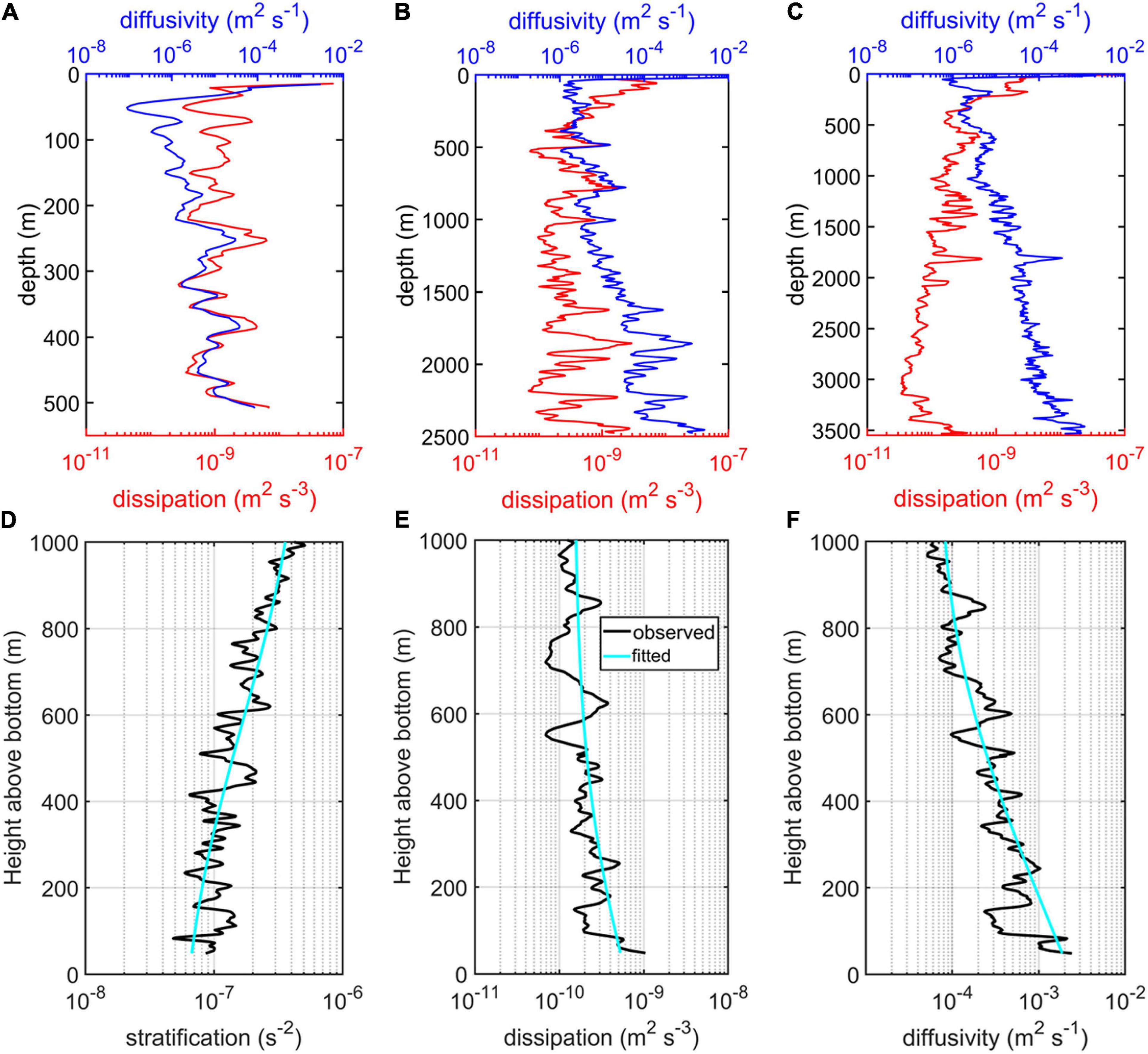
Figure 2. (A–C) Full-depth turbulent dissipation profiles (red solid lines) and diffusivity profiles (blue solid lines) obtained from the VMP instruments at the seamount corresponding to the VMP stations P1, P2, and P3, respectively. (D–F) Display the height above bottom averaged stratification, turbulent dissipation, and diffusivity profile, respectively, at the seamount corresponding to the depth range below 100-m height above the bottom of two deep turbulent mixing stations. The black solid lines display the observed results and the cyan lines the fitted results.
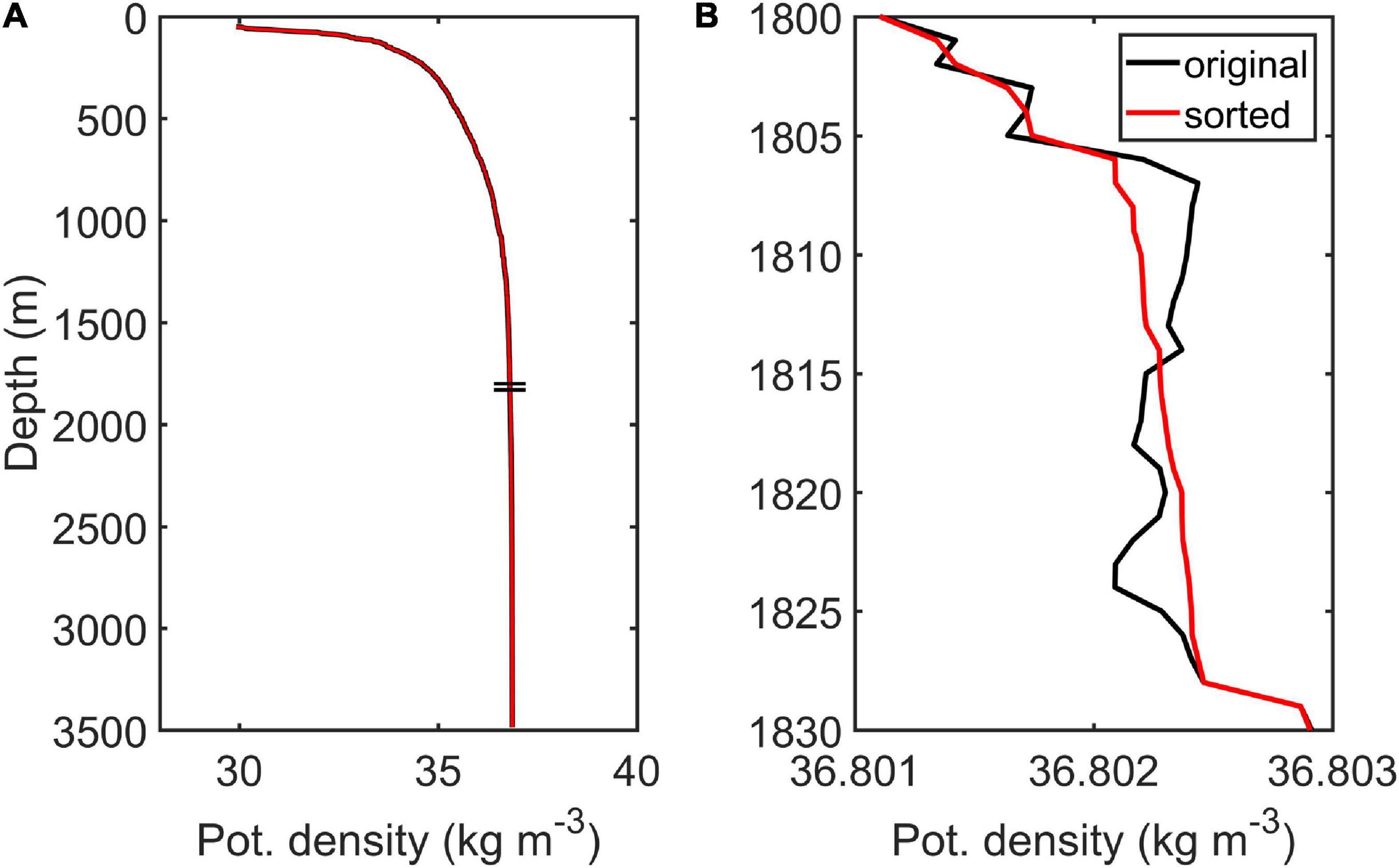
Figure 3. (A) Profile of the potential density (reference pressure of 2,000 dbar) obtained from station P3 at the seamount. (B) Profile of the potential density corresponding to the depth range indicated by the two black horizontal lines in panel (A). The black curve indicates the original potential density profile, whereas the red curve indicates the sorted potential density.
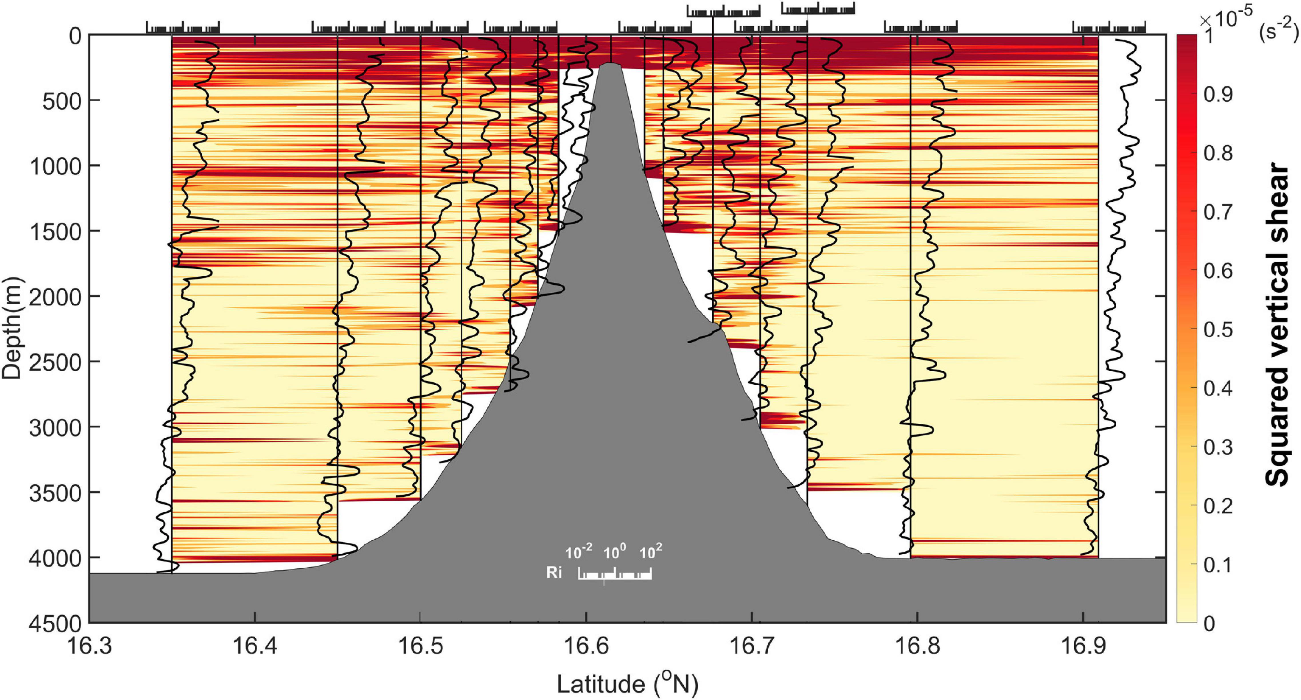
Figure 4. Spatial distributions of the squared vertical shear (colors) and Richardson number Ri = N2/S2 (black profiles) acquired from CTD and LADCP profiling along the meridional section of the seamount. The scale for Ri is given at the lower center and redrawn above each profile with a vertical line indicating Ri = 0.25.
For turbulent diffusivity, Figure 2 suggests concurrent intensification toward the bottom below the surface mixed layer, with the diffusivity on shallow profile (P1) reaching 1 × 10⁻⁴ m2 s–1 and that on the other two profiles (P2 and P3) reaching up to 1 × 10⁻³ m2 s–1, which is two orders of magnitude above the typical levels in the deep ocean interior (Gregg, 1987; Ledwell et al., 1993; Kunze and Sanford, 1996); this finding is consistent with the results of Toole et al. (1997). Hydrographic data around the seamount revealed enhanced velocity vertical shear near the bottom (Figure 4). Large velocity shears and deep weak stratification provide favorable conditions for developing shear instability, and thus local turbulent mixing when Richardson number (Ri = N2/S2, where ) falls below a critical value of 0.25. Profiles of Richardson number around the seamount show that values of Richardson number decrease toward the bottom and become less than 0.25 at some depths in the upslope direction of the seamount (Figure 4), indicative of the upslope variations in turbulent mixing at the seamount.
Previous studies similarly reported enhanced turbulent diffusivity of O (10–3 m2 s–1) in the deep northeastern SCS and Zhongsha Islands, mainly due to the dissipation of internal tides (e.g., Tian et al., 2009; Zhou et al., 2014; Yang et al., 2016). Locally generated high-mode internal tides tend to dissipate when encountering small-scale topographic features (e.g., Kunze and Smith, 2004; Cimoli et al., 2019; Vic et al., 2019), resulting in the local enhancement of turbulent mixing. To obtain the internal tidal signals around the seamount, we have applied the harmonic analysis (Godin, 1972) to the raw velocity of the two deep moorings and high-resolution LADCP and the baroclinic velocities are acquired by subtracting depth-averaged velocity from the raw velocity. When extracting internal tides from the LADCP data, we assumed that there is no spatial variability in the internal tides along the observation section of the seamount. Although previous studies pointed out that the propagation and dissipation of internal tides could be influenced by the critical latitudes where the inertial frequency equals the tidal frequency (Robertson et al., 2017; Dong et al., 2019), the effective inertial frequency (considering the relative vorticity of the background current) corresponding to the latitude of the seamount was estimated to be about 6.5 × 10⁻⁶ s–1 and is relatively smaller than the frequency of the diurnal internal tide around the seamount estimated to be approximately 1.2 × 10⁻⁵ s–1. In this way, the propagation or dissipation of the internal tides around the seamount should not be influenced by the critical latitude effects. But internal tide around the complex rough topography could have a change with its propagation due to its dissipation or radiation near the complex rough topography (Zhao, 2014; Xu et al., 2016; Hibiya et al., 2017). Nevertheless, the assumption could reasonably provide us a glimpse of the vertical structure of internal tides around the seamount, though it could make the estimates of internal tides potentially deviating from the realistic situation of internal tides around the seamount. Finally, energetic baroclinic diurnal and semidiurnal internal tides around the seamount were revealed by the velocity data of deep moorings and LADCP, and their maximum magnitude of velocity can reach 12.34 and 3.72 cm s–1, respectively (Figures 5, 6). It is reasonable to speculate that the local dissipation of internal tides near the bottom could be the main contributor to the bottom-intensified turbulent mixing around the seamount. Wavelet analysis of the fine-resolution bathymetry of the seamount reveals a couple of small-scale rough topographic features on the slope of the seamount (Figure 7C), one of which corresponds well with P2. This could be the reason that turbulent dissipation at the bottom of P2 dominates over that of P3. In short, inhomogeneously distributed bottom-intensified turbulent mixing is revealed in the upslope direction of the seamount, and this intensified mixing could be closely related to local complicated small-scale topographic features.
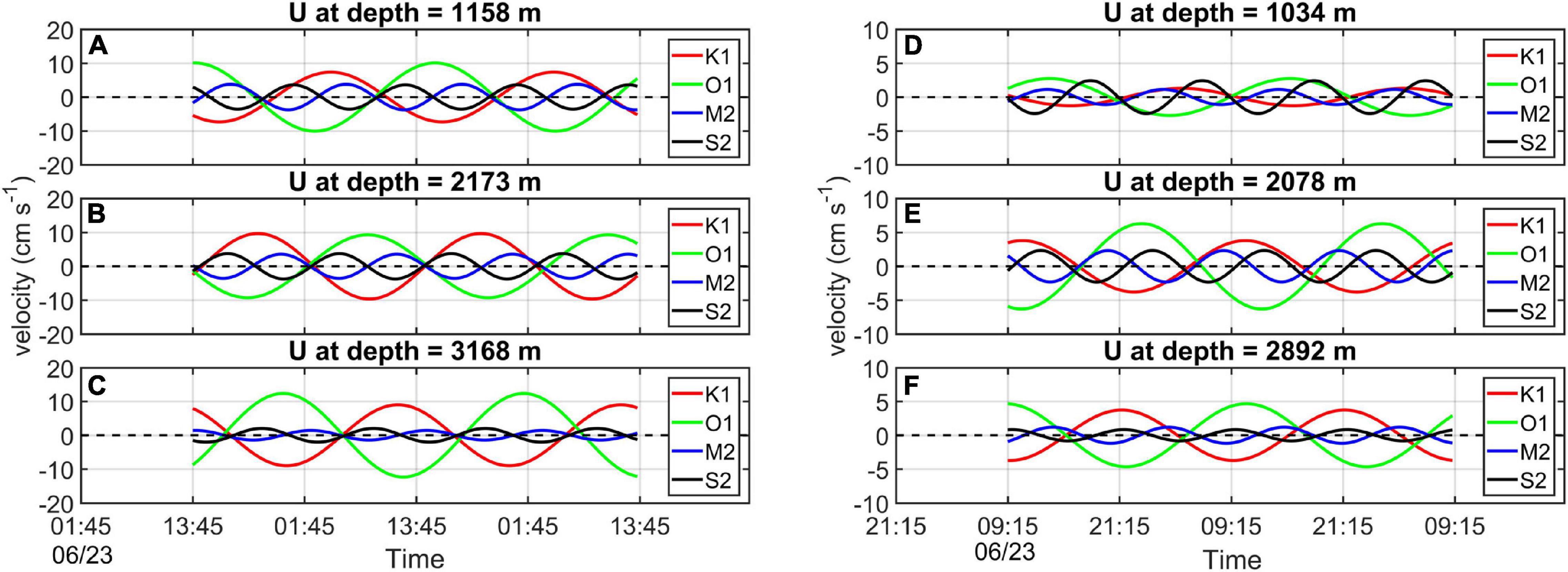
Figure 5. (A–C) Internal tide components acquired from the deep mooring located on the northern slope of the seamount. (D–F) Internal tide components acquired from the deep mooring located on the southern slope of the seamount.
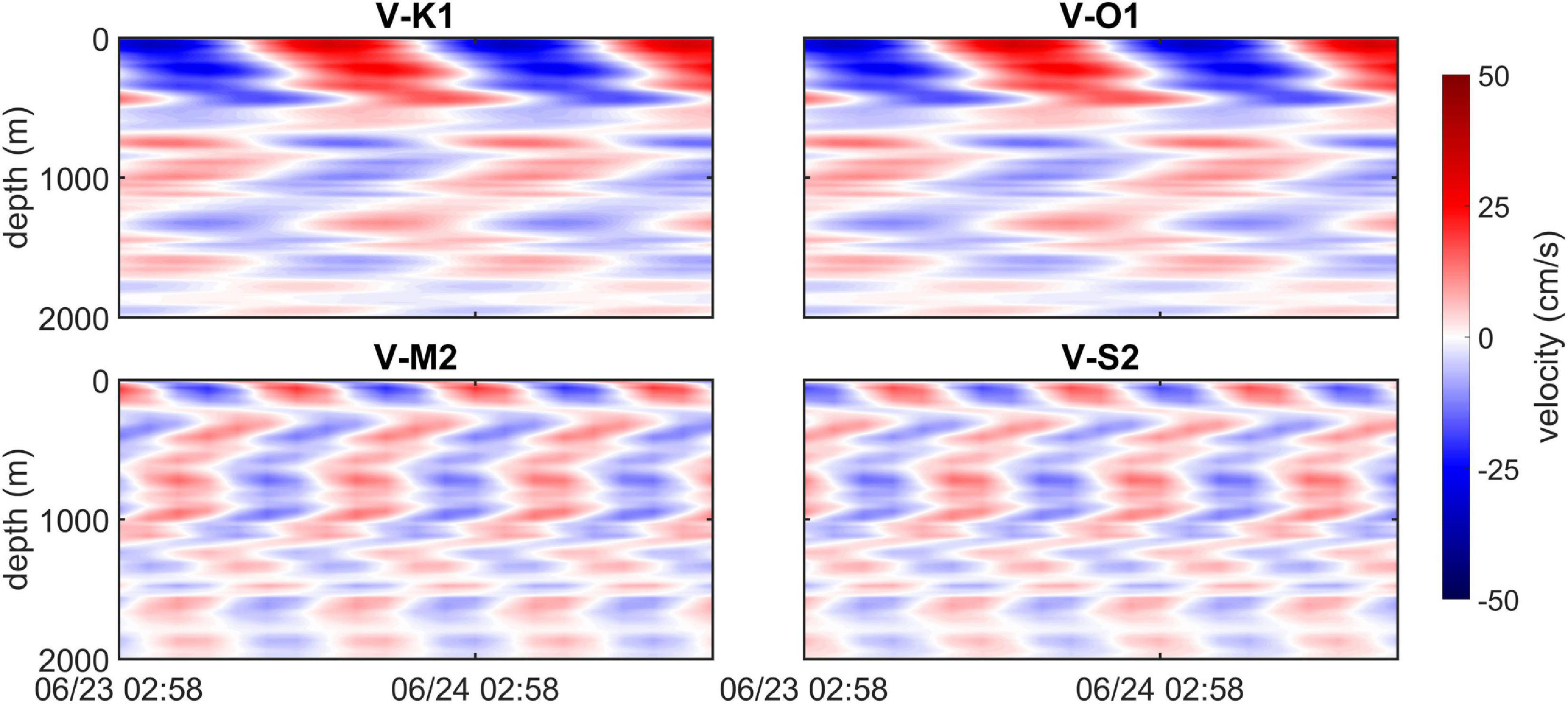
Figure 6. Baroclinic internal tide components were acquired from the LADCP profiles cast along the south–north section of the seamount.
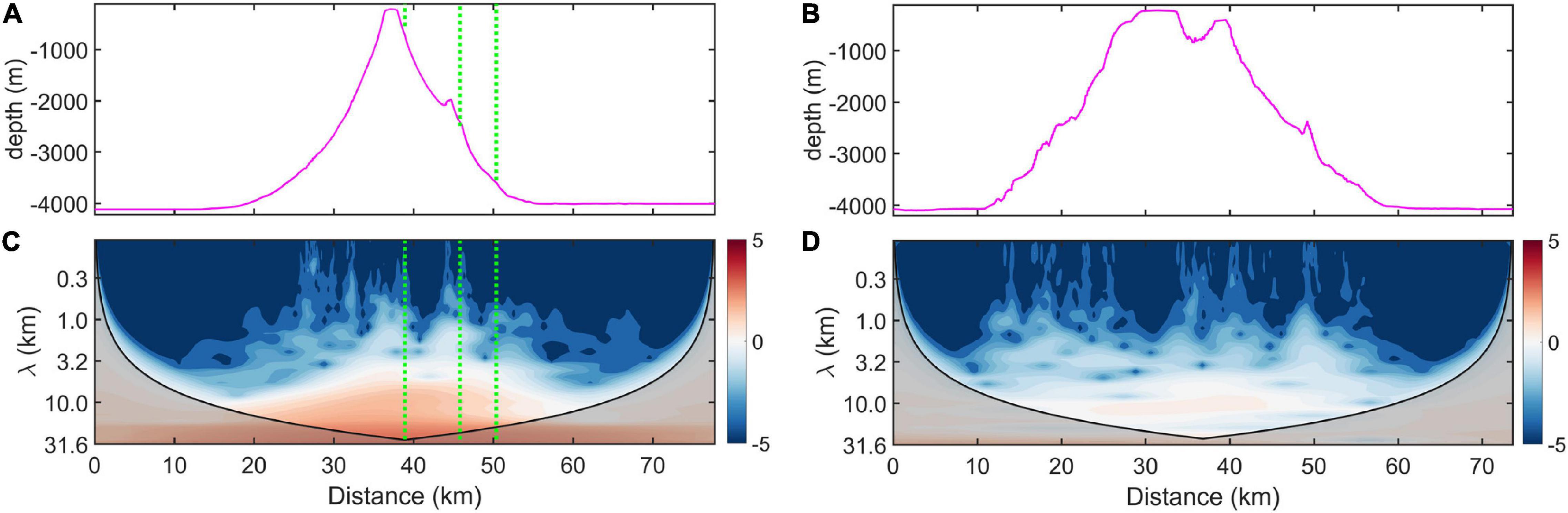
Figure 7. (A,B) Topographic profiles of the meridional and zonal sections of the seamount, respectively. (C,D) Wavelet analyses of the topography of the corresponding sections. The color-filled contours are the log10-scaled variance (m2) of the wavelet transform of the normalized topography. The black solid line in each panel indicates that the area below is subjected to the edge effect. The vertical green dotted lines indicate the positions of the VMP profiles.
In situ observations in this study revealed that there exist upslope variations in turbulent mixing at the seamount topography. To investigate the impact of inhomogeneously distributed turbulent mixing on the circulation around the seamount, three numerical experiments (Exp1–Exp3) are conducted. Exp1 is configured with three-dimensional turbulent mixing and vertical turbulent diffusivity profiles depending only on the local height above the bottom (Figure 8A), whereas Exp2 is configured with one local hump of bottom-intensified turbulent diffusivity in the upslope direction (Figure 8D), and Exp3 is configured with two isolated local humps of bottom-intensified turbulent diffusivity in the upslope direction (Figure 8G). The vertical profile of turbulent diffusivity imposed in the three experiments is obtained by exponentially fitting mean vertical profiles of the observed turbulent diffusivity acquired by averaging near-bottom profiles of P2 and P3 on a height above the bottom (hab) coordinate (Figure 2F). To get some knowledge of the upslope structure of turbulent diffusivity at the seamount, we applied MacKinnon-Gregg (MG) parameterization (MacKinnon and Gregg, 2003) to reveal the spatial distribution of turbulent diffusivity at the seamount due to that estimates of MG parameterization can generally predict the magnitude and variability of the deep turbulent diffusivity at the seamount (Figures 9B,D). The MG parameterization can be expressed as follows:
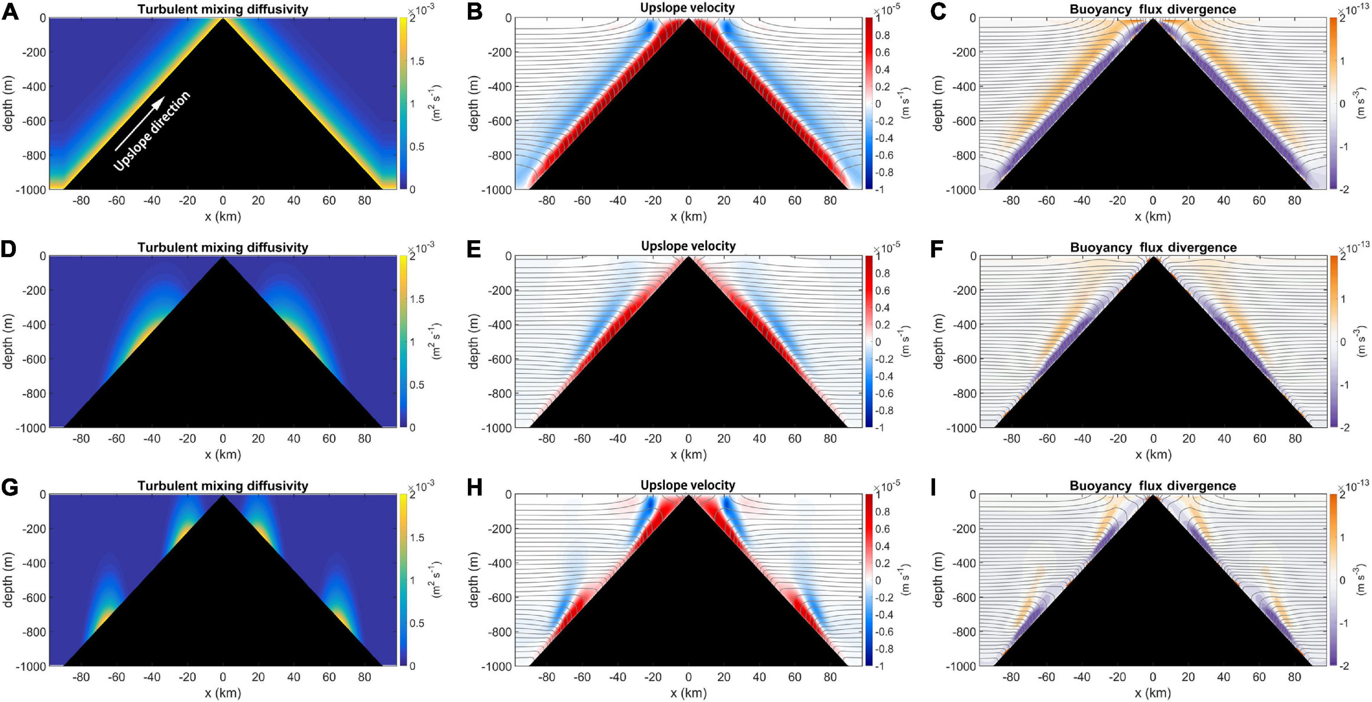
Figure 8. (A,D,G) Spatial distributions of the turbulent diffusivity applied in the model experiments corresponding to Exp1, Exp2, and Exp3, respectively. (B,E,H) Spatial distributions of the upslope velocity of Exp1, Exp2, and Exp3, respectively. (C,F,I) Spatial distributions of the turbulent buoyancy flux resulting from the bottom-intensified turbulent mixing around the conic seamount corresponding to Exp1, Exp2, and Exp3, respectively. The upslope direction is indicated by the white arrow in panel (A).
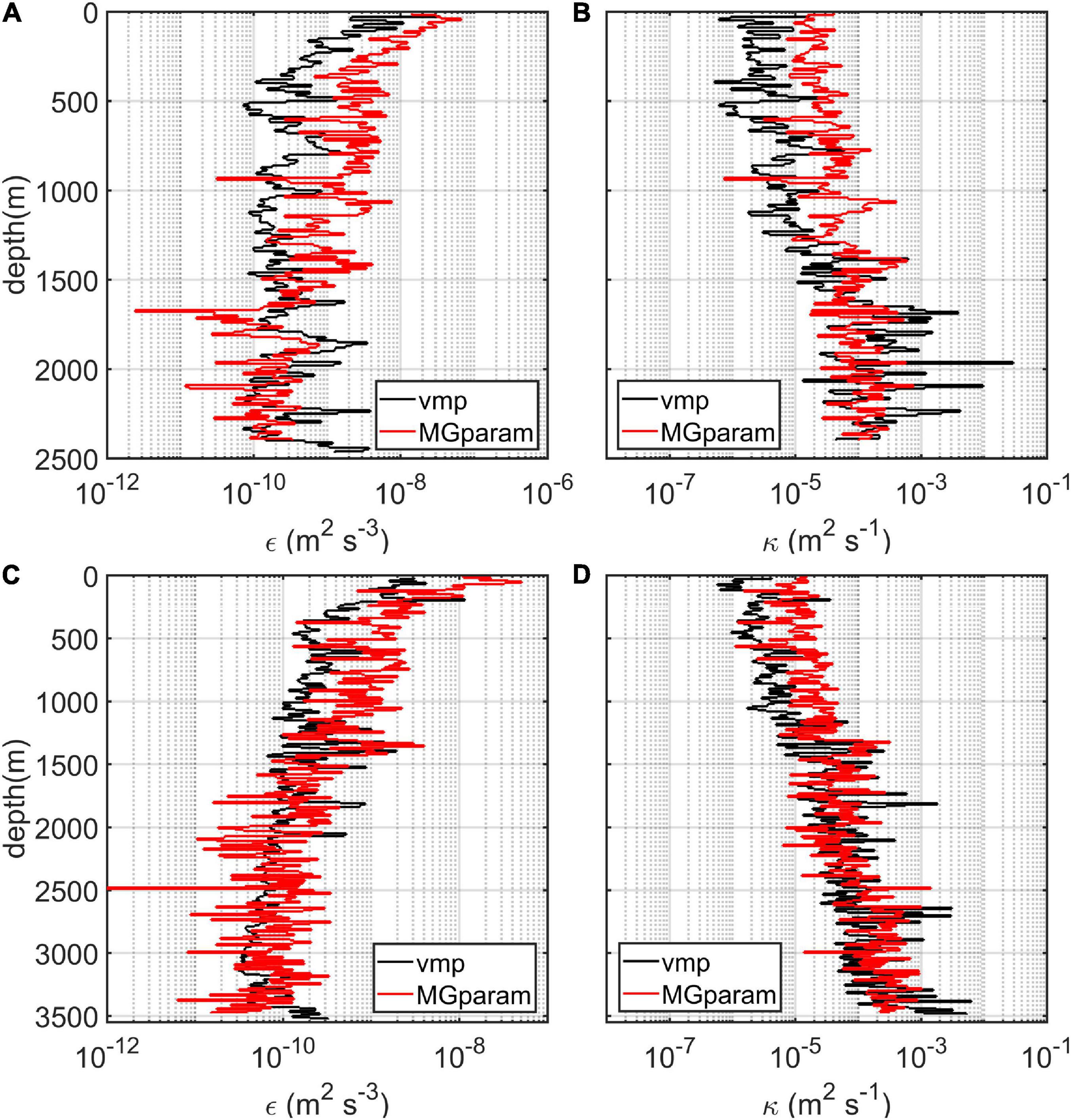
Figure 9. (A,B) Profiles of the turbulent dissipation rate and diffusivity from the observations (black solid lines) and MG parameterization (red solid lines) at P2. (C,D) Similar profiles except at P3.
where S0 = N0 = 5.2 × 10⁻³ s–1 and ε0 = 4.0 × 10⁻⁹ m2 s–3, which is adopted here to adjust the parameterized turbulent dissipation rate to the observed data (Figures 9A,C). Quantitatively, the differences in turbulent diffusivity between VMP observations and MG parameterization are almost within a factor of 2–4, which suggests that MG parameterization can yield reasonable estimates of the turbulent diffusivity around the seamount and can provide reliable support to explore the upslope structure of deep turbulent diffusivity around the seamount. The success of MG parameterization should owe to that velocity shear in our study area mainly came from low-frequency internal waves such as diurnal and semidiurnal waves (Figures 5, 6), which was similar to features of the internal wave field over the New England Shelf, where the MG parameterization was derived initially. Also, the applicability of MG parameterization over rough topography in the SCS has also been examined by Liang et al. (2017), Shang X.D. et al. (2017), and Sun et al. (2018). To make full use of the results of VMP observations and MG parameterization, we configured the field of turbulent diffusivity of a model experiment by combining the results of VMP observations (Figure 2F) and MG parameterization (Figures 10B,D). The full-depth profiles of turbulent diffusivity are provided by the VMP observations while relatively high-resolution upslope structures of turbulent diffusivity near the bottom are estimated by MG parameterization (Figures 10A,C). Then, the upslope structure of the applied bottom-intensified turbulent diffusivity is established based on the fitting relationship between the near-bottom turbulent diffusivity estimated from the MG parameterization and the upslope distance (Figures 10B,D). Finally, the MG parameterization reveals one local turbulent diffusivity peak near the bottom in the upslope direction on the north slope of the seamount (Figure 10B) and two local turbulent diffusivity peaks in the upslope direction on the south slope of the seamount (Figure 10D); these results reflect a heterogeneous distribution of turbulent diffusivity in the upslope direction of the seamount. Hence, the turbulent diffusivity fields imposed in Exp2 and Exp3 are configured with unimodal and bimodal fitting structures, respectively, as shown in Figure 8. When the bottom-intensified turbulent mixing is prescribed in the model, the isopycnals near the sloping bottom boundary tend to tilt due to the insulating boundary conditions and thus produce pressure gradient forces that subsequently drive the flows. The local available potential energy that energizes the mean flows is produced by the vertical buoyancy flux generated by the prescribed turbulent mixing acting on the background stratification.
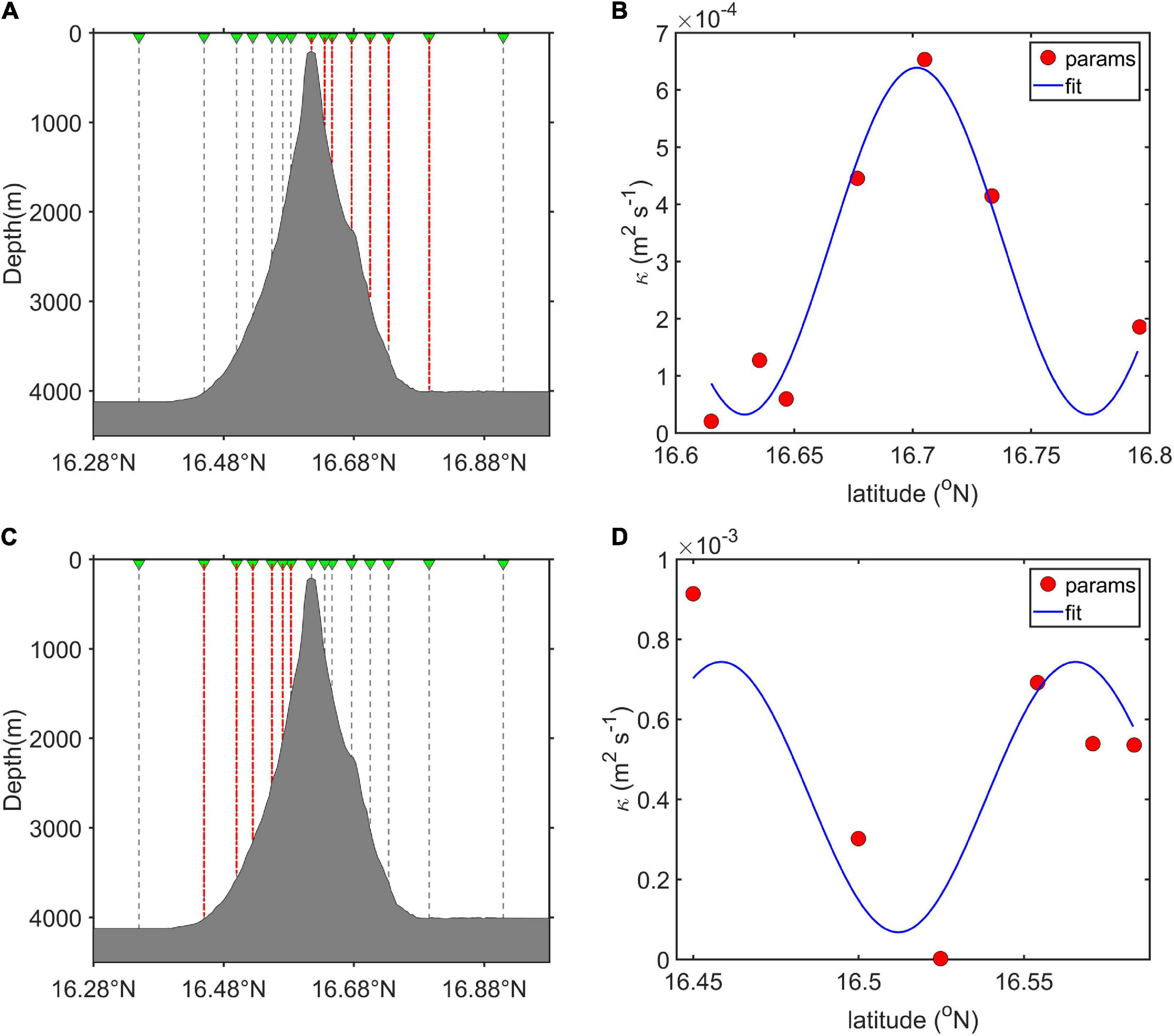
Figure 10. (A,C) Locations of the observed CTD profiles along the meridional section of the seamount in the SCS. (B,D) Upslope distributions of the turbulent diffusivity near the bottom of the north slope and south slope corresponding to the CTD profiles indicated by the red dashed lines in panels (A,C), respectively. The red dots indicate the turbulent diffusivity near the bottom estimated by the MG parameterization, and the blue solid line is a sine-function fitted result.
The results of Exp1 expose significant convergence of the turbulent buoyancy flux in the BBL and divergence outside the BBL (Figure 8C). Accordingly, upslope flow occurs in the BBL, whereas widespread but relatively weak downslope flow exists outside the BBL (Figure 8B). Obviously, with the turbulent diffusivity depending only on the local height above the bottom, the spatial distribution of the dipolar flow is uniform in the upslope direction of the seamount, which is consistent with the findings of previous studies (Ferrari et al., 2016; McDougall and Ferrari, 2017).
However, the topographic slope of a realistic seamount generally features small-scale rough features, which are indicative of one or more local enhancements of bottom-intensified turbulent mixing in the upslope direction of the seamount (Figures 7, 10B,D). In Exp2 with the bottom-intensified turbulent diffusivity exhibiting one hump in the upslope direction of the seamount (Figure 8D), the tilt of isopycnals near the sloping bottom increases corresponding to the hump of bottom-intensified turbulent mixing (Figure 8E). The diapycnal dipolar flow is locally strengthened (Figure 8E), which corresponds to the intensified convergence of the turbulent buoyancy flux in the BBL and divergence outside the BBL (Figure 8F). For Exp3, in which two isolated turbulent diffusivity humps exist in the upslope direction of the seamount (Figure 8G), the diapycnal flow exhibits a pattern similar to that in Exp2 except that two local strengthened diapycnal dipolar flows exist near the boundary layer (Figure 8H). With locally strengthened diapycnal upwelling motions in the BBL, the divergence and convergence of upslope water transport in the BBL could result in the exchange of water between the BBL and the deep ocean interior. In this way, the intrusion of water from the boundary into the interior modulates the water stratification and affects the pattern of large-scale circulation in the interior. Thus, the pattern of diapycnal dipolar flow near the boundary layer of the seamount is highly sensitive to the upslope structure of bottom-intensified turbulent mixing.
In Exp1, driven by homogeneous bottom-intensified turbulent mixing, corresponding to the tilting of isopycnals (Figure 8B), the horizontal flow satisfies the thermal wind balance and displays an anticyclonic flow pattern away from the BBL of the seamount (Figure 11A), whereas the horizontal flow inside the thin BBL of the seamount displays a cyclonic pattern (Figure 11A). The horizontal flow around the seamount has an order of 10–3 m s–1, which is significantly larger than that of the diapycnal dipolar flow [O (10–5 m–2 s–1)] driven by bottom-intensified turbulent mixing. By considering the variability of enhanced mixing in the upslope direction of the seamount, the thickness of the BBL exhibits substantial variability in the upslope direction. Furthermore, the local enhancement of bottom-intensified turbulent mixing could notably elevate the BBL (Figures 8E,H). Nevertheless, cyclonic and anticyclonic flow patterns still exist within and outside the BBL, respectively, and are locally strengthened corresponding to the hump of bottom-intensified turbulent mixing in the upslope direction (Figures 11C,E).
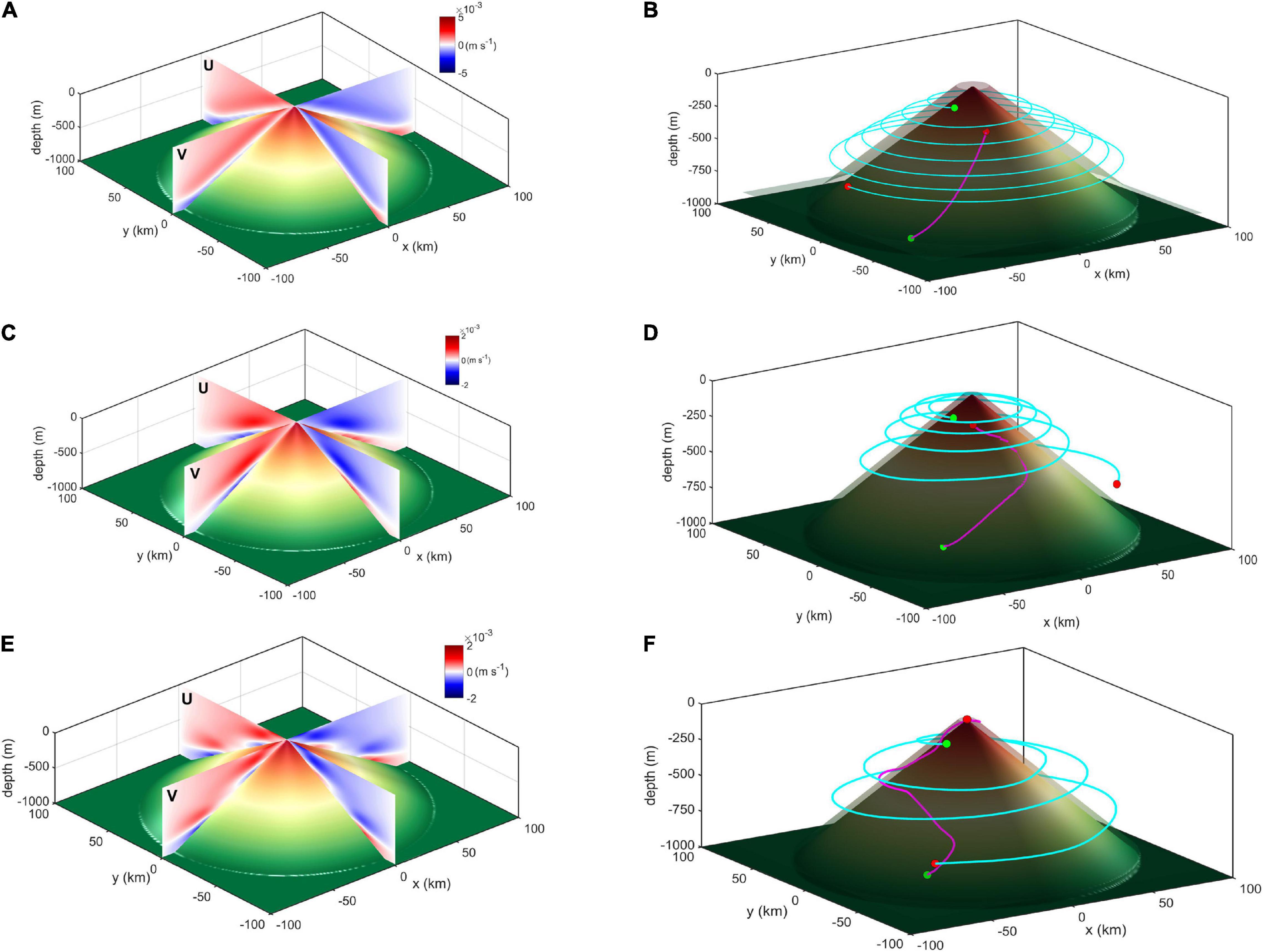
Figure 11. (A,C,E) Three-dimensional horizontal flow driven by the bottom-intensified turbulent mixing around the seamount of Exp1, Exp2, and Exp3, respectively (displayed in Figures 8A,D,G). (B,D,F) Upward spiraling pathway of fluid particles (magenta solid line) in the BBL and downward spiraling pathway of fluid particles (cyan solid line) outside the BBL of Exp1, Exp2, and Exp3, respectively, with the green dot indicating the start point and the red dot indicating the endpoint.
The trajectories of fluid particles driven by bottom-intensified turbulent mixing are calculated by considering both the upslope and the horizontal flows around the seamount. In Exp1, the trajectories of the fluid particles display an anticyclonic spiral-down pattern outside the BBL, whereas the fluid particles in the BBL upwell cyclonically around the seamount (Figure 11B). This suggests that deepwater upwelling through the BBL around the seamount does not ascend linearly but rather along an upward spiraling pathway. When the bottom-intensified turbulent mixing is locally enhanced in the upslope direction (Exp2 and Exp3), the fluid particles in the BBL experience complex upward spiraling pathways. When cyclonic spiral-up fluid particles in the BBL enter the region where turbulent mixing is locally enhanced and the convergence of bottom water occurs, the particles escape from the BBL into the region dominated by anticyclonic flow and exhibit an anticyclonic spiral-up trajectory (Figures 11D,F). In summary, regulated by the inhomogeneously distributed bottom-intensified turbulent mixing in the upslope direction of the seamount, the notable exchange of bottom waters between the BBL and deep ocean interior is related to the upward and downward spiraling pathways of bottom waters manifesting as complicated three-dimensional circulation around the seamount.
In fact, variations in upslope water transport driven by boundary mixing depend on many factors, for example, temporal variations in boundary mixing, background stratification, and bottom slope. Here, we mainly concentrated on the effect of the upslope structure of bottom-intensified turbulent mixing on shaping the structure of circulation around the seamount topography. Previous studies have focused on the effect of background stratification (Phillips et al., 1986) and bottom slope (Dell and Pratt, 2015; McDougall and Ferrari, 2017; Holmes et al., 2018) on the upslope water transport driven by boundary mixing. To better understand the modulation mechanism of deep circulation around the seamount, further studies should be conducted on the effect of the temporal variations in turbulent mixing, background stratification, and the slope of the bottom topography on the circulation around the seamount.
Based on in situ observations around a seamount in the SCS, we revealed that bottom-intensified turbulent mixing around the seamount exhibits an inhomogeneous structure in the upslope direction, which could be closely related to the small-scale rough topographic features of the seamount slope. In fact, various oceanic processes are capable of producing local enhanced turbulent mixing such as internal tides, submesoscale eddies, and geostrophic flow. Previous studies pointed out that strong barotropic tides flowing across sloping topography can generate beams of internal tides propagating into deeper water (deWitt et al., 1986; New, 1988; Pingree and New, 1989). The fact that turbulent mixing is locally enhanced along a beam of internal tides has been reported in many previous studies (Lueck and Mudge, 1997; Lien and Gregg, 2001; Tang et al., 2021). The local hotspots of turbulent mixing have also been found to exist over the continental slope that is near-critical for semidiurnal frequencies (Nash et al., 2004, 2007). In addition, numerical experiments in this study indicate that the structure of the regional circulation around the seamount is highly sensitive to the spatial distribution of this bottom-intensified turbulent mixing. When bottom-intensified turbulent mixing is locally enhanced in the upslope direction, the diapycnal dipolar flow featuring upwelling motion in the BBL and downwelling motion outside the BBL is strengthened correspondingly. Consequently, the local convergence and divergence of waters in the BBL of the seamount result in the exchange of water between the boundary and the deep ocean interior. As the model simulations evolve, bottom-intensified turbulent mixing gradually erodes the bottom stratification while away from the bottom, the interior stratification is strengthened at some depths and weakened at others as fluid is drawn into or forced out of the boundary layer due to the divergence or convergence of upslope water transport in the BBL (Figure 12). Subsequently, the interior circulation will be modulated with the penetration of the stratification effect of the boundary layer on the interior field. The effect of exchange between the boundary layer and interior on the evolution of the interior stratification was also explored by Dell and Pratt (2015). On the other hand, multiple locally enhanced horizontal anticyclonic (cyclonic) circulations outside (inside) the BBL around the seamount are generated by locally enhanced bottom-intensified turbulent mixing in the upslope direction. By tracking the particle motions around the seamount, we find that deep water around the seamount could diabatically upwell to the surface through the BBL along a cyclonic upward spiraling pathway. A more complex upwelling pathway of deep water through the BBL of the seamount could occur when the bottom-intensified turbulent mixing becomes locally enhanced in the upslope direction.
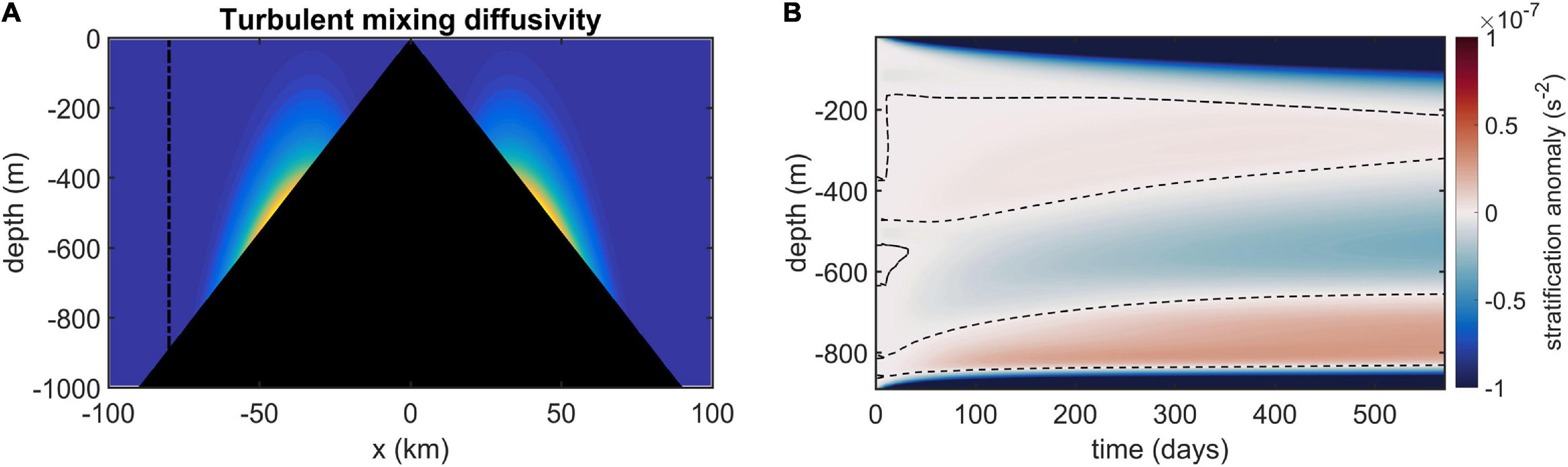
Figure 12. (A) Spatial distributions of the turbulent diffusivity applied in the model experiment Exp2. (B) The evolution of stratification anomaly (relative to the initial stratification) in the column is indicated with a dashed line in panel (A). The thin dashed lines in panel (B) indicate the value of zero.
Although our study is inspired from in situ observations, the model simulations were conducted relying on a number of ideal assumptions. For example, due to the utility of the initial constant background stratification, the buoyancy flux in the model simulations will result in a more tilting profile than that in the real system with strong vertical decay in the observed background stratification, which subsequently results in quantitative differences between results of model simulations and the real situation at the seamount. Nevertheless, we expect that this change will only impact the magnitude of the velocities and not their structure. In addition, the persistent upslope structure of turbulent diffusivity around the seamount topography was utilized in our model simulations with ignorance of the temporal variability of turbulent mixing around the seamount. Different upslope structures of turbulent mixing around the seamount might be revealed with a varying phase of internal tides (MacKinnon and Gregg, 2005; Palmer et al., 2015; Sun et al., 2016; van Haren, 2018; Yang et al., 2021). When taking into consideration temporal variations of turbulent mixing around the rough topography, the realistic situation around the seamount topography in the ocean is doomed to be more complex than the results of our study. The above-mentioned assumptions are open to question, but they allow us a glimpse of the effect that variations in the upslope structure of turbulent mixing will have on the structure of circulation around the seamount topography.
Mooring observations around the seamount in this study also display an anticyclonic horizontal flow pattern with a notable baroclinic structure (Figure 13). Both of the two deep moorings are located at the northern perimeter of a cyclonic eddy based on sea level anomaly observations (not shown here), suggesting a northwestward background current in the upper layer. This indicates that the anticyclonic horizontal flow revealed by two deep moorings around the seamount is not directly associated with the upper ocean processes. Also, the effects of tidal residual current on the anticyclonic mean flow were evaluated. Based on the estimating formula of tidal residual velocity used by Freeland (1994), the magnitudes of tidal residual velocity around the seamount were estimated to be 0.90 cm s–1 due to the diurnal tides and 0.02 cm s–1 due to the semidiurnal tides, which were relatively smaller than the observed background mean velocity of 4.2 cm s–1. The direction of tidal residual current was complex depending on the far field flow patterns (Pingree and Maddock, 1985). Considering the estimated small magnitude of tidal residual velocity around the seamount, we speculated that the rectification effects of tidal residual current could not change the anticyclonic mean flow pattern around the seamount revealed in this study. In fact, previous studies suggested that this anticyclonic horizontal circulation could be induced by a geostrophic current flowing over an isolated seamount, thereby its potential vorticity conserved (Smith, 1979). On the other hand, MacCready and Rhines (1991) pointed out that the boundary mixing could drive an upslope flow that reaches a steady value after a decay time scale or shutdown time and also produce a simultaneous along-slope velocity in the boundary layer and the along-slope velocity would be diffused into the interior with time. Finally, the velocities of background interior flow are affected and tend to approach the magnitude of the diffused along-slope velocity induced by boundary mixing (Thorpe, 1987; MacCready and Rhines, 1991). The upslope and along-slope velocities driven by boundary mixing are also revealed in our study, of which the shutdown time is estimated to be about 12 model days based on the model setup, and the results of model experiments after 500 model days are displayed in this study. Therefore, the anticyclonic circulation suggested by the observations resulting from either the bottom intensified mixing or the inflow, or the contributions from both processes, still needs to be further investigated with more specifically designed observations and model experiments.
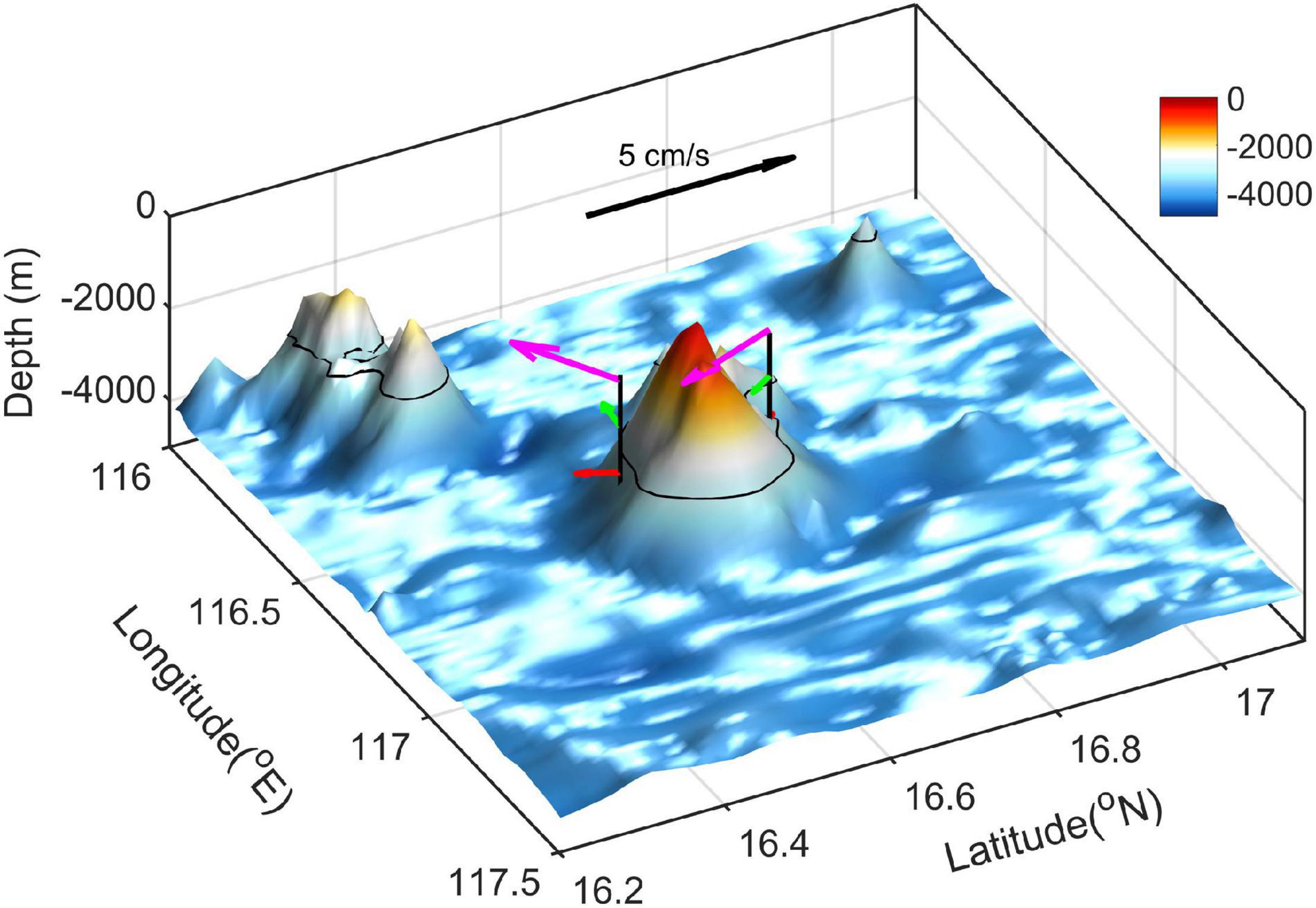
Figure 13. Mean velocity vector obtained from the two deep moorings located on the slope of the seamount in the SCS. The arrows with different colors indicate the mean velocity vector of different depth, and the black lines represent the 3,000-m isobaths.
In conclusion, this study explored the spatial structure of circulation and turbulent mixing around a seamount in the SCS based on in situ observations, and we revealed that the three-dimensional circulation around the seamount is modulated by the inhomogeneous turbulent mixing in the upslope direction of the seamount. However, the modeling experiments do not consider variations in the slope of bottom topography and stratification, which might be additional key factors in modulating the flow structure around a seamount (Phillips et al., 1986; Dell and Pratt, 2015; Holmes et al., 2018), and thus are worthy of further investigation. Additionally, ideally persistent turbulent mixing is considered in this study, whereas turbulent mixing in the realistic ocean is temporary, and the extent of the horizontal velocity driven by near-bottom boundary turbulent mixing could penetrate into the interior with time (MacCready and Rhines, 1991). Further systematic studies should be conducted on the effect of the spatial distribution of turbulent mixing and the slope of the bottom topography on the circulation around a seamount, which has considerable significance for exploring the mechanism by which the large-scale circulation around seamounts is modulated. On the other hand, they can provide a new perspective for studying the distributions of ocean nutrients and marine life affected by the dynamic processes around seamounts.
Bathymetry data of the SCS are acquired from global seafloor topography (https://topex.ucsd.edu/cgi-bin/get_data.cgi). The data analyzed in this study can be obtained at the following website: https://jmp.sh/ylfsynW.
RY performed the data analysis and wrote the manuscript. CZ conceived the study and contributed to the editing of the manuscript. JT initiated the idea of the study. All authors contributed to the analysis of the results and writing the manuscript.
This work was supported by the National Natural Science Foundation of China (Grant Nos. 91858203, 91958205, 42076027, 41630970, and 41876022), the major project from Sanya Yazhou Bay Science and Technology City Administration (Grant No. SKJC-KJ-2019KY04). VMP casts were collected onboard of R/V “Jia Geng” implementing the open research cruise NORC2018-06 supported by NSFC Shiptime Sharing Project (Grant No. 41749906).
The authors declare that the research was conducted in the absence of any commercial or financial relationships that could be construed as a potential conflict of interest.
All claims expressed in this article are solely those of the authors and do not necessarily represent those of their affiliated organizations, or those of the publisher, the editors and the reviewers. Any product that may be evaluated in this article, or claim that may be made by its manufacturer, is not guaranteed or endorsed by the publisher.
Callies, J., Ferrari, R., Klymak, J. M., and Gula, J. (2015). Seasonality in submesoscale turbulence. Nat. Commun. 6:6862. doi: 10.1038/ncomms7862
Carter, G. S., Gregg, M. C., and Merrifield, M. A. (2006). Flow and mixing around a small seamount on Kaena Ridge, Hawaii. J. Phys. Oceanogr. 36, 1036–1052. doi: 10.1175/JPO2924.1
Cimoli, L., Caulfield, C. P., Johnson, H. L., Marshall, D. P., Mashayek, A., Garabato, A. C. N., et al. (2019). Sensitivity of deep ocean mixing to local internal tide breaking and mixing efficiency. Geophys. Res. Lett. 46, 14622–14633. doi: 10.1029/2019GL085056
de Lavergne, C., Madec, G., Le Sommer, J., Nurser, A. J. G., and Naveira Garabato, A. C. (2016). The impact of a variable mixing efficiency on the abyssal overturning. J. Phys. Oceanogr. 46, 663–681. doi: 10.1175/JPO-D-14-0259.1
Dell, R., and Pratt, L. (2015). Diffusive boundary layers over varying topography. J. Fluid Mech. 769, 635–653. doi: 10.1017/jfm.2015.88
deWitt, L. M., Levine, M. D., Paralson, C. A., and Burt, W. W. (1986). Semidiurnal internal tide in JASIN: observations and simulation. J. Geophys. Res. 91, 2581–2592. doi: 10.1029/jc091ic02p02581
Dong, J., Robertson, R., Dong, C., Hartlipp, P. S., Zhou, T., Shao, Z., et al. (2019). Impacts of mesoscale currents on the diurnal critical latitude dependence of internal tides: a numerical experiment based on Barcoo Seamount. J. Geophys. Res. Oceans 124, 2452–2471. doi: 10.1029/2018JC014413
Drake, H. F., Ferrari, R., and Callies, J. (2020). Abyssal circulation driven by near-boundary mixing: water mass transformations and interior stratification. J. Phys. Oceanogr. 50, 2203–2226. doi: 10.1175/JPO-D-19-0313.1
Ferrari, R., Mashayek, A., McDougall, T. J., Nikurashin, M., and Campin, J.-M. (2016). Turning ocean mixing upside down. J. Phys. Oceanogr. 46, 2239–2261. doi: 10.1175/JPO-D-15-0244.1
Freeland, H. (1994). Ocean circulation at and near Cobb Seamount. Deep Sea Res. Part I Oceanogr. Res. Pap. 41, 1715–1732. doi: 10.1016/0967-0637(94)90069-8
Garrett, C. (2003). Internal tides and ocean mixing. Science 301, 1858–1859. doi: 10.1126/science.1090002
Gregg, M., D’Asaro, E., Riley, J., and Kunze, E. (2018). Mixing efficiency in the ocean. Annu. Rev. Mar. Sci. 10, 443–473. doi: 10.1146/annurev-marine-121916-063643
Gregg, M. C. (1987). Diapycnal mixing in the thermocline: a review. J. Geophys. Res. 92, 5249–5286. doi: 10.1029/JC092iC05p05249
Gregg, M. C., d’Asaro, E. A., Shay, T. J., and Larson, N. (1986). Observations of persistent mixing and near-inertial internal waves. J. Phys. Oceanogr. 16, 856–885. doi: 10.1175/1520-0485(1986)016<0856:oopman>2.0.co;2
Hibiya, T., Ijichi, T., and Robertson, R. (2017). The impacts of ocean bottom roughness and tidal flow amplitude on abyssal mixing. J. Geophys. Res. Oceans 122, 5645–5651. doi: 10.1002/2016JC012564
Holmes, R. M., de Lavergne, C., and McDougall, T. J. (2018). Ridges, seamounts, troughs, and bowls: topographic control of the dianeutral circulation in the abyssal ocean. J. Phys. Oceanogr. 48, 861–882. doi: 10.1175/JPO-D-17-0141.1
Holmes, R. M., and McDougall, T. J. (2020). Diapycnal transport near a sloping bottom boundary. J. Phys. Oceanogr. 50, 3253–3266. doi: 10.1175/JPO-D-20-0066.1
Huang, R. X., and Jin, X. (2002). Deep circulation in the South Atlantic induced by bottom-intensified mixing over the midocean ridge. J. Phys. Oceanogr. 32, 1150–1164. doi: 10.1175/1520-0485(2002)032<1150:dcitsa>2.0.co;2
Kitchingman, A., Lai, S., Morato, T., and Pauly, D. (2007). “How many seamounts are there and where are they located?,” in Seamounts: Ecology, Fisheries & Conservation, eds T. J. Pitcher, T. Morato, P. J. B. Hart, M. R. Clark, N. Haggan, and R. S. Santos (Hoboken, NJ: Wiley), 26–40. doi: 10.1002/9780470691953
Kunze, E., MacKay, C., McPhee-Shaw, E. E., Morrice, K., Girton, J. B., and Terker, S. R. (2012). Turbulent mixing and exchange with interior waters on sloping boundaries. J. Phys. Oceanogr. 42, 910–927. doi: 10.1175/JPO2926.1
Kunze, E., and Sanford, T. B. (1996). Abyssal mixing: where it is not. J. Phys. Oceanogr. 26, 2286–2296. doi: 10.1175/1520-0485(1996)026<2286:amwiin>2.0.co;2
Kunze, E., and Smith, S. G. L. (2004). The role of small-scale topography in turbulent mixing of the global ocean. Oceanography 17, 55–64. doi: 10.5670/oceanog.2004.67
Lavelle, J., Lozovatsky, I., and Smith, D. (2004). Tidally induced turbulent mixing at Irving Seamount—modeling and measurements. Geophys. Res. Lett. 31:L10308. doi: 10.1029/2004GL019706
Ledwell, J. R., Montgomery, E. T., Polzin, K. L., Laurent, L. C. S., Schmitt, R. W., and Toole, J. M. (2000). Evidence for enhanced mixing over rough topography in the abyssal ocean. Nature 403, 179–182. doi: 10.1038/35003164
Ledwell, J. R., Watson, A. J., and Law, C. S. (1993). Evidence for slow mixing across the pycnocline from an open-ocean tracer-release experiment. Nature 364, 701–703. doi: 10.1038/364701a0
Liang, C. R., Chen, G. Y., and Shang, X. D. (2017). Observations of the turbulent kinetic energy dissipation rate in the upper central South China Sea. Ocean Dyn. 67, 597–609. doi: 10.1007/s10236-017-1051-6
Lien, R. C., and Gregg, M. (2001). Observations of turbulence in a tidal beam and across a coastal ridge. J. Geophys. Res. 106, 4575–4591. doi: 10.1029/2000JC000351
Lueck, R. G., and Mudge, T. D. (1997). Topographically induced mixing around a shallow seamount. Science 276, 1831–1833. doi: 10.1126/science.276.5320.1831
MacCready, P., and Rhines, P. B. (1991). Buoyant inhibition of Ekman transport on a slope and its effect on stratified spin-up. J. Fluid Mech. 223, 631–661. doi: 10.1017/s0022112091001581
MacKinnon, J. A., and Gregg, M. C. (2003). Shear and baroclinic energy flux on the summer New England shelf. J. Phys. Oceanogr. 33, 1462–1475. doi: 10.1175/1520-0485(2003)033<1462:sabefo>2.0.co;2
MacKinnon, J. A., and Gregg, M. C. (2005). Spring mixing: turbulence and internal waves during restratification on the New England shelf. J. Phys. Oceanogr. 35, 2425–2443. doi: 10.1175/jpo2821.1
Marshall, J., Adcroft, A., Hill, C., Perelman, L., and Heisey, C. (1997a). A finite-volume, incompressible Navier Stokes model for studies of the ocean on parallel computers. J. Geophys. Res. 102, 5753–5766. doi: 10.1029/96JC02775
Marshall, J., Hill, C., Perelman, L., and Adcroft, A. (1997b). Hydrostatic, quasi-hydrostatic, and nonhydrostatic ocean modeling. J. Geophys. Res. 102, 5733–5752. doi: 10.1029/96JC02776
McDougall, T. J. (1989). “Dianeutral advection, paper presented at Parameterization of Small-Scale Processes,” in Proceedings of the ‘Aha Huliko ‘a Hawaiian Winter Workshop, Honolulu, HI.
McDougall, T. J., and Ferrari, R. (2017). Abyssal upwelling and downwelling driven by near-boundary mixing. J. Phys. Oceanogr. 47, 261–283. doi: 10.1175/JPO-D-16-0082.1
Munk, W., and Wunsch, C. (1998). Abyssal recipes II: energetics of tidal and wind mixing. Deep Sea Res. I 45, 1977–2010. doi: 10.1016/S0967-0637(98)00070-3
Munk, W. H. (1966). Abyssal recipes. Deep Sea Res. Oceanogr. Abstr. 13, 707–730. doi: 10.1016/0011-7471(66)90602-4
Nash, J. D., Kunze, E., Toole, J. M., Martini, K., and Kelly, S. (2007). Hotspots of deep ocean mixing on the Oregon continental slope. Geophys. Res. Lett. 34:L01605. doi: 10.1029/2006GL028170
Nash, J. D., Kunze, E., Toole, J. M., and Schmitt, R. W. (2004). Internal tide reflection and turbulent mixing on the continental slope. J. Phys. Oceanogr. 34, 1117–1134. doi: 10.1175/1520-0485(2004)034<1117:itratm>2.0.co;2
Naveira Garabato, A. C., Polzin, K. L., King, B. A., Heywood, K. J., and Visbeck, M. (2004). Widespread intense turbulent mixing in the Southern Ocean. Science 303, 210–213. doi: 10.1126/science.1090929
New, A. L. (1988). Internal tidal mixing in the Bay of Biscay. Deep Sea Res. 35, 691–709. doi: 10.1016/0198-0149(88)90026-x
Osborn, T. (1980). Estimates of the local rate of vertical diffusion from dissipation measurements. J. Phys. Oceanogr. 10, 83–89. doi: 10.1038/s41598-020-74938-5
Palmer, M. R., Stephenson, G. R., Inall, M. E., Balfour, C., Düsterhus, A., and Green, J. A. M. (2015). Turbulence and mixing by internal waves in the Celtic Sea determined from ocean glider microstructure measurements. J. Mar. Syst. 144, 57–69. doi: 10.1016/j.jmarsys.2014.11.005
Perfect, B., Kumar, N., and Riley, J. J. (2020). Energetics of seamount wakes. Part I: energy exchange. J. Phys. Oceanogr. 50, 1365–1382. doi: 10.1175/jpo-d-19-0105.1
Peters, H., Gregg, M., and Toole, J. (1988). On the parameterization of equatorial turbulence. J. Geophys. Res 93, 1199–1218. doi: 10.1029/JC093iC02p01199
Phillips, O. M., Shyu, J. H., and Salmun, H. (1986). An experiment on boundary mixing - Mean circulation and transport rates. J. Fluid Mech. 173, 473–499. doi: 10.1017/s0022112086001234
Pingree, R. D., and Maddock, L. (1985). Rotary currents and residual circulation around banks and islands. Deep Sea Res. Part A Oceanogr. Res. Pap. 32, 929–947. doi: 10.1016/0198-0149(85)90037-8
Pingree, R. D., and New, A. L. (1989). Downward propagation of internal tidal energy into the Bay of Biscay. Deep Sea Res. 36, 735–758. doi: 10.1016/0198-0149(89)90148-9
Polzin, K., Toole, J., Ledwell, J., and Schmitt, R. (1997). Spatial variability of turbulent mixing in the abyssal ocean. Science 276, 93–96. doi: 10.1126/science.276.5309.93
Robertson, R., Dong, J., and Hartlipp, P. (2017). Diurnal Critical latitude and the latitude dependence of internal tides, internal waves, and mixing based on Barcoo seamount. J. Geophys. Res. Oceans 122, 7838–7866. doi: 10.1002/2016JC012591
Ruan, X., and Callies, J. (2020). Mixing-driven mean flows and submesoscale eddies over mid-ocean ridge flanks and fracture zone canyons. J. Phys. Oceanogr. 50, 175–195. doi: 10.1175/JPO-D-19-0174.1
Ruan, X., Thompson, A. F., Flexas, M. M., and Sprintall, J. (2017). Contribution of topographically generated submesoscale turbulence to Southern Ocean overturning. Nat. Geosci. 10, 840–845. doi: 10.1038/ngeo3053
Shang, X., Qi, Y., Chen, G., Liang, C., Lueck, R. G., Prairie, B., et al. (2017). An expendable microstructure profiler for deep ocean measurements. J. Atmos. Oceanic Technol. 34, 153–165. doi: 10.1175/JTECH-D-16-0083.1
Shang, X. D., Liang, C. R., and Chen, G. Y. (2017). Spatial distribution of turbulent mixing in the upper ocean of the South China Sea. Ocean Sci. 13, 503–519. doi: 10.5194/os-13-503-2017
Shay, T. J., and Gregg, M. (1986). Convectively driven turbulent mixing in the upper ocean. J. Phys. Oceanogr. 16, 1777–17982. doi: 10.1175/1520-0485(1986)016<1777:cdtmit>2.0.co;2
Smith, R. B. (1979). The influence of mountains on the atmosphere. Adv. Geophys. 21, 87–230. doi: 10.1016/S0065-2687(08)60262-9
Smith, W. H. F., and Sandwell, D. T. (1997). Global sea floor topography from satellite altimetry and ship depth soundings. Science 277, 1956–1962. doi: 10.1126/science.277.5334.1956
St. Laurent, L. C., Toole, J. M., and Schmitt, R. W. (2001). Buoyancy forcing by turbulence above rough topography in the Abyssal Brazil Basin. J. Phys. Oceanogr. 31, 3476–3495. doi: 10.1175/1520-0485
Stewart, K. D., Hughes, G. O., and Griffiths, R. W. (2012). The role of turbulent mixing in an overturning circulation maintained by surface buoyancy forcing. J. Phys. Oceanogr. 42, 1907–1922. doi: 10.1175/JPO-D-11-0242.1
Sun, H., Yang, Q., Zhao, W., Liang, X., and Tian, J. (2016). Temporal variability of diapycnal mixing in the northern South China Sea. J. Geophys. Res. Oceans 121, 8840–8848. doi: 10.1002/2016jc012044
Sun, H., Yang, Q. X., and Tian, J. W. (2018). Microstructure measurements and finescale parameterization assessment of turbulent mixing in the northern South China Sea. J. Oceanogr. 74, 485–498. doi: 10.1007/s10872-018-0474-0
Tang, Q., Jing, Z., Lin, J., and Sun, J. (2021). Diapycnal mixing in the subthermocline of the mariana ridge from high-resolution seismic images. J. Phys. Oceanogr. 51, 1283–1300. doi: 10.1175/jpo-d-20-0120.1
Thorpe, S. A. (1987). Current and temperature variability on the continental slope. Philos. Trans. R. Soc. Lond. 323A, 471–517. doi: 10.1098/rsta.1987.0100
Tian, J., Yang, Q., and Zhao, W. (2009). Enhanced diapycnal mixing in the South China Sea. J. Phys. Oceanogr. 39, 3191–3203. doi: 10.1175/2009JPO3899.1
Toole, J. M., Schmitt, R. W., and Polzin, K. L. (1994). Estimates of diapycnal mixing in the abyssal ocean. Science 264, 1120–1123. doi: 10.1126/science.264.5162.1120
Toole, J. M., Schmitt, R. W., Polzin, K. L., and Kunze, E. (1997). Near-boundary mixing above the flanks of a midlatitude seamount. J. Geophys. Res. 102, 947–959. doi: 10.1029/96JC03160
van Haren, H. (2018). Abyssal plain hills and internal wave turbulence. Biogeosciences 15, 4387–4403. doi: 10.5194/bg-15-4387-2018
Vic, C., Naveira Garabato, A. C., Green, J. A. M., Waterhouse, A. F., Zhao, Z., Melet, A., et al. (2019). Deep-ocean mixing driven by small-scale internal tides. Nat. Commun. 10:2099. doi: 10.1038/s41467-019-10149-5
Wain, D. J., and Rehmann, C. R. (2010). Transport by an intrusion generated by boundary mixing in a lake. Water Resour. Res. 46:W08517. doi: 10.1029/2009WR008391
Waterhouse, A. F., MacKinnon, J. A., Nash, J. D., Alford, M. H., Kunze, E., Simmons, H. L., et al. (2014). Global patterns of diapycnal mixing from measurements of the turbulent dissipation rate. J. Phys. Oceanogr. 44, 1854–1872. doi: 10.1175/jpo-d-13-0104.1
Wessel, P., Sandwell, D. T., and Kim, S.-S. (2010). The global seamount census. Oceanography 23, 24–33. doi: 10.5670/oceanog.2010.60
Wunsch, C., and Ferrari, R. (2004). Vertical mixing, energy, and the general circulation of the oceans. Annu. Rev. Fluid Mech. 36, 281–314. doi: 10.1146/annurev.fluid.36.050802.122121
Xu, J., Xie, J., Chen, Z., Cai, S., and Long, X. (2012). Enhanced mixing induced by internal solitary waves in the South China Sea. Cont. Shelf Res. 49, 34–43. doi: 10.1016/j.csr.2012.09.010
Xu, Z., Liu, K., Yin, B., Zhao, Z., Wang, Y., and Li, Q. (2016). Long-range propagation and associated variability of internal tides in the South China Sea. J. Geophys. Res. Oceans 121, 8268–8286. doi: 10.1002/2016JC012105
Yang, C. F., Chi, W. C., and van Haren, H. (2021). Deep-sea turbulence evolution observed by multiple closely spaced instruments. Sci. Rep. 11:3919. doi: 10.1038/s41598-021-83419-2
Yang, Q., Nikurashin, M., Sasaki, H., Sun, H., and Tian, J. (2019). Dissipation of mesoscale eddies and its contribution to mixing in the northern South China Sea. Sci. Rep. 9:556. doi: 10.1038/s41598-018-36610-x
Yang, Q., Zhao, W., Liang, X., and Tian, J. (2016). Three-dimensional distribution of turbulent mixing in the South China Sea. J. Phys. Oceanogr. 46, 769–788. doi: 10.1175/JPO-D-14-0220.1
Zhang, Z., Liu, Z., Richards, K., Shang, G., Zhao, W., Tian, J., et al. (2019). Elevated diapycnal mixing by a subthermocline eddy in the western equatorial Pacific. Geophys. Res. Lett. 46, 2628–2636. doi: 10.1029/2018GL081512
Zhao, Z. (2014). Internal tide radiation from the Luzon Strait. J. Geophys. Res. Oceans 119, 5434–5448. doi: 10.1002/2014JC010014
Keywords: circulation, bottom-intensified turbulent mixing, bottom boundary layer, seamount, South China Sea
Citation: Ye R, Shang X, Zhao W, Zhou C, Yang Q, Tian Z, Qi Y, Liang C, Huang X, Zhang Z, Guan S and Tian J (2022) Circulation Driven by Multihump Turbulent Mixing Over a Seamount in the South China Sea. Front. Mar. Sci. 8:794156. doi: 10.3389/fmars.2021.794156
Received: 13 October 2021; Accepted: 25 November 2021;
Published: 06 January 2022.
Edited by:
Robin Robertson, Xiamen University Malaysia, MalaysiaReviewed by:
Zhiqiang Liu, Southern University of Science and Technology, ChinaCopyright © 2022 Ye, Shang, Zhao, Zhou, Yang, Tian, Qi, Liang, Huang, Zhang, Guan and Tian. This is an open-access article distributed under the terms of the Creative Commons Attribution License (CC BY). The use, distribution or reproduction in other forums is permitted, provided the original author(s) and the copyright owner(s) are credited and that the original publication in this journal is cited, in accordance with accepted academic practice. No use, distribution or reproduction is permitted which does not comply with these terms.
*Correspondence: Chun Zhou, Y2h1bnpob3VAb3VjLmVkdS5jbg==
Disclaimer: All claims expressed in this article are solely those of the authors and do not necessarily represent those of their affiliated organizations, or those of the publisher, the editors and the reviewers. Any product that may be evaluated in this article or claim that may be made by its manufacturer is not guaranteed or endorsed by the publisher.
Research integrity at Frontiers
Learn more about the work of our research integrity team to safeguard the quality of each article we publish.