 Xintao Jiang
 Junbiao Tu
 Daidu Fan
- 1State Key Laboratory of Marine Geology, Tongji University, Shanghai, China
- 2Laboratory of Marine Geology, Qingdao National Laboratory for Marine Science and Technology, Qingdao, China
Hydrodynamic responses of the aquaculture farm structures have been increasingly studied because of their importance in informing the aquaculture carrying capacity and ecological sustainability. The hydrodynamical effect of the suspended cage farm on flow structures and vertical mixing in the Sansha Bay, SE China, is examined using observational data of two comparative stations inside and outside the cage farm. The results show that current velocities are relatively uniform in the vertical except a bottom boundary layer outside the cage farm. Within the cage farm, the surface boundary layer produced by the cage-induced friction is obvious with current velocities decreasing upward, combining the classic bottom boundary layer to form a “double-drag layers” structure in the water column. The cage-induced drag decreases with water depth in the surface boundary layer with a maximum thickness of 3/4 the water column, and the current velocities can be reduced by 54%. The cage-induced friction can also significantly hinder the horizontal water exchange in the farm. Periodic stratification phenomena exist at both stations under the influence of lateral circulation. However, the subsurface (5–10 m below the sea surface) water column below the cage facilities is well-mixed as indicated by the vertical density profile, where the velocity shear (10–3 m–2) is about 10 times higher than that of the subsurface layer outside the cage farm. Therefore, we speculate that the well-mixing of the subsurface water column results from the local turbulence induced by the velocity shear, which in turn is produced by the friction of cage structures.
Introduction
Marine aquaculture is expanding rapidly in recent decades to satisfy the sustainable protein demand of the growing human population [Naylor et al., 2000; Food and Agriculture Organization [FAO], 2018; Cabre et al., 2021]. However, the rapid development of inshore aquaculture has been increasingly criticized for its adverse impact on ambient water settings. The presence of large aquaculture farm structures should greatly affect the flow structures, water exchange capacity, and nutrient circulation (Holmer et al., 2002; Wu et al., 2017; Weitzman et al., 2019; Visch et al., 2020). The production of huge organic substances (e.g., residual bait, feces, and metabolic waste) in the aquaculture area is potential to trigger the occurrence of eutrophication, red tide, and hypoxia (Newton et al., 2016; Leary et al., 2017). These impacts may have a knock-on effect on the carrying capacity of aquaculture farms, which ultimately affects the surrounding ecology and its ecosystem services (Ferreira et al., 2014; Ottinger et al., 2016; Cabre et al., 2021). China accounts for over 60% of global aquaculture production with a rapidly growing aquaculture industry, commonly using floating cages, longlines, and other structures to cultivate aquatic organisms. Chemical and ecological impacts of the vast scale of suspended aquaculture have been well studied in China, but physical impacts remain relatively understudied (Wartenberg et al., 2017). Hydrodynamic response of the aquaculture farm structures or canopies has been increasingly studied because of its importance in informing how to maintain healthy ecosystems.
Flow velocities inside and around the cage nets can be significantly reduced (Zhao et al., 2013a,b), mainly due to the shielding effects downstream the cage nets (Bi et al., 2014a). The flow velocity reduction effect can also be influenced by the cage number and the cage arrangement (Zhao et al., 2013b,2015). Another effect of the cage on local hydrodynamics is wave attenuation by the cage. Bi et al. (2017) observed that the maximum attenuation of wave transmission coefficient was approximately 7% downstream of the cage using a three-dimensional computational fluid dynamic model. Bi et al. (2014b) investigated the interaction between the flow and a net cage with a flexible net using a numerical model. They reported that the increase in incoming velocity will aggravate the deformation of the cage, and the deformed net has more noticeable blockage effect than the net with no deformation.
In addition to the cage-induced flow -reduction in a horizontal direction, the vertical distribution of flow velocity can also be modified by the presence of the cage. A number of studies have shown that the surface velocities are greatly reduced by the canopies, and the maximum velocities appear in the middle or lower layers of the water column (Fan et al., 2009; Herrera et al., 2018). Lin et al. (2016) observed flow attenuation of 75–90% at the top layer in a longline mussel farm in Zhoushan, China. Pilditch et al. (2001) observed a 40% reduction in current velocity inside a suspended scallop aquaculture farm in Nova Scotia, Canada. Plew et al. (2006) demonstrated similar reductions within a mussel farm of Golden Bay, New Zealand. Based on the observations and model outputs, O’Donncha et al. (2017) reported that current velocities inside the farm structure were obviously reduced, but the flow was accelerated beneath the canopy. In addition, the existence of aquaculture facilities significantly increases the exchange cycle of water. Wang et al. (2018) found the retention time of water increased by 25–40 days in the inner bay and 5–10 days in the middle of Sanggou Bay due to the resistance of farm structures. These flow responses undoubtedly impact the nutrient supply and carrying capacity of the system.
Aquaculture activities can also affect the stratification and mixing patterns of the aquatic environment (Zhao et al., 2017; Xu and Dong, 2018). Plew et al. (2006) found that the dissipation rate at the canopy interface was greater than that at the bottom in the mussel aquaculture farm of Golden Bay, indicating that the local turbulence generated at the canopy interface enhanced mixing. The flume experiment conducted by Plew (2011a) in the laboratory showed that the existence of canopy was conducive to the development of shear layer processes at the canopy interface, resulting in turbulence and the enhanced mixing. However, the observations in giant kelp forests in Santa Cruz, California, showed that the small shear of highly decreased current velocity due to the canopy effect was difficult to impede the water stratification (Rosman et al., 2007). Stevens and Petersen (2011) found that the dissipation rate of turbulent kinetic energy inside the aquaculture farm was only 10–8–10–6 m2s–3. It is therefore indicated that the impacts of aquaculture structures on stratification and mixing are not affirmatory for the turbulence generation or suppression.
Under the complex topographic conditions, such as estuaries and bays, the factors affecting the vertical stratification and mixing are even more complicated (Huguenard et al., 2015; Tu et al., 2019; Xiao et al., 2019). Simpson et al. (1990) found that the periodic stratification (i.e., enhanced mixing at flood and more stratification at ebb) was mainly controlled by longitudinal tidal straining in tidal estuaries. But Lacy et al. (2003) observed the opposite phenomenon in San Francisco Bay, where the stratification increased during the flood tide and decreased during the ebb tide, due to the lateral circulation. Liu and Huguenard (2020) demonstrated that the periodic stratification in the oyster aquaculture farm, Damariscotta River in the NE, United States, was mainly controlled by the lateral circulation and less affected by the aquaculture facilities.
This study aims to evaluate the impact of cage aquaculture farms on the local hydrodynamics in Sansha Bay, a semienclosed bay in Fujian, SE China (Figure 1). The water quality and ecosystem of the bay have been degrading in recent decades due to increasing aquaculture (Sun et al., 2015). The influence of cage aquaculture on the flow field and water exchange in Sansha Bay was investigated based on observations and model output (Lin et al., 2019). The near-surface current velocity that squared in the cage-free areas was much larger than that inside the cage farms by a factor exceeding three in deep channels, and by a factor of two in tidal flats. The cage-induced drag could reach as deep as 20 m in the relatively deep channels. Cage aquaculture significantly increased the exchange cycle of water in the bay. However, the hydrodynamic response of the dense aquaculture facilities in the bay has so far not been studied by the comparison of dual campaigning sites, one inside and the other outside the cage farm. We describe the method including the study site, and data collection and processing in Section 2. The main results are presented in Section 3. The hydrodynamic change by the cage-induced drag and the potential mechanisms influencing stratification and mixing are discussed in Section 4. Section 5 summarizes the conclusions.
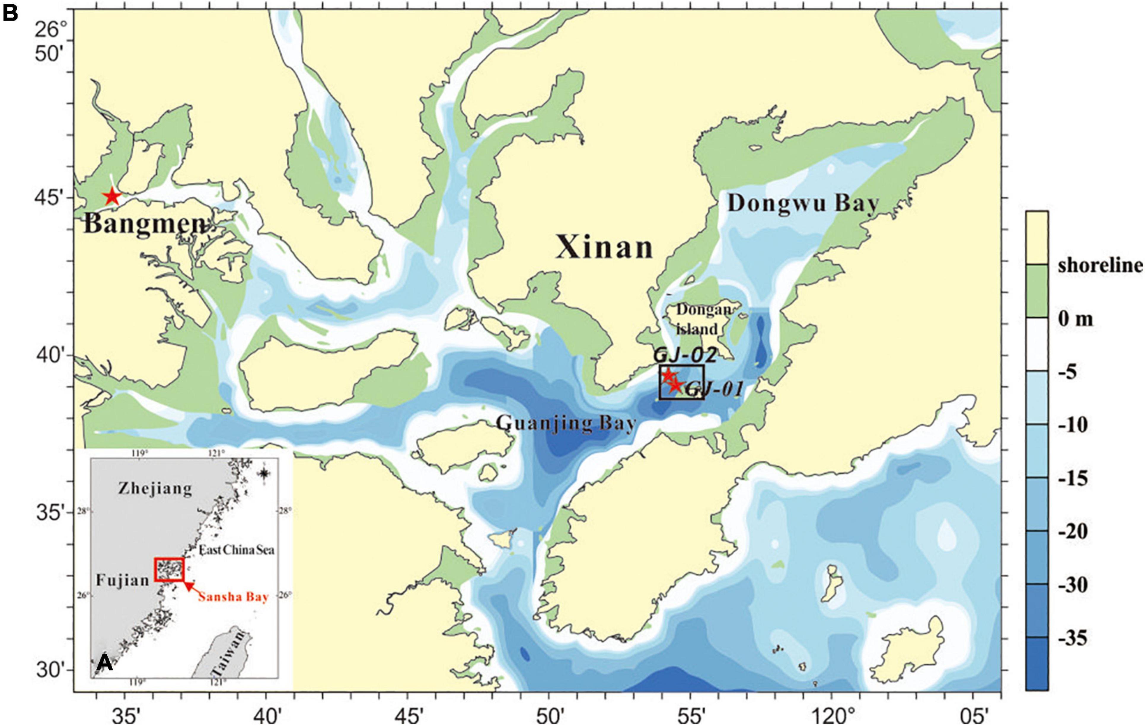
Figure 1. (A) Location of the Sansha Bay in the East China Sea and (B) Bathymetric map of the Sansha Bay with the tide-gauging station at Bangmen and the two campaigning sites: GJ-01 (inside the cage farm) and GJ-02 (outside the farm). The red stars indicate the locations of observation sites.
Materials and Methods
Study Site
Sansha Bay is a semienclosed bay consisting of several secondary bays (Figure 1B). The bay has a total area of approximately 675 km2, and is connected to the East China Sea through a deep, narrow channel of approximately 3 km wide. It is dominated by regular semidiurnal tides with a maximum tidal range of 5.64 m. The local currents are also significantly affected by tides, and the maximum current speed exceeds 1 m/s in the deep channels but decreases below 0.5 m/s in the shallow areas (Lin et al., 2017). The wave climate is calm with an annual wave height of 0.1 m and an average wind speed of 3.2 m/s. Affected by freshwater input, the bayhead is characterized by warmer and less-salty water, whereas the bay mouth is mainly influenced by the colder and saltier seawater (Lin et al., 2016).
The Sansha Bay has an aquaculture area of ∼ 300 km2. According to the Google map digitization, the longline aquaculture farms for seaweeds are distributed over a much larger area in the shallow and inner bay whereas the cage aquaculture farms for fish are mainly distributed around the Guanjing Bay (Figure 2A) where deeper channels are located with stronger currents (Figure 1B; Lin et al., 2017). There are about 20 × 22 fish cages in an aquaculture unit adjacent to the observation site GJ-01, and the distance between two adjacent units is about 20–30 m (Figure 2C). A standard cage is 3 m in both length and width and 4 m in height, and they float at the sea surface under the help of plastic foam and wood, and also bottom-mounted anchor lines (Figure 2B). The bar length of the net used in cage aquaculture is 32.8 mm and the diameter is 5.6 mm. The young fish begins to be cultured in spring (April to May) or in autumn (October to December) (about 10,000 individuals/cage). When the yellow croaker grows up to 10 cm in length, the aquaculture density decreases to 1,500 individuals/cage, and it grows to the standard of commercial fish for about 10–15 months.
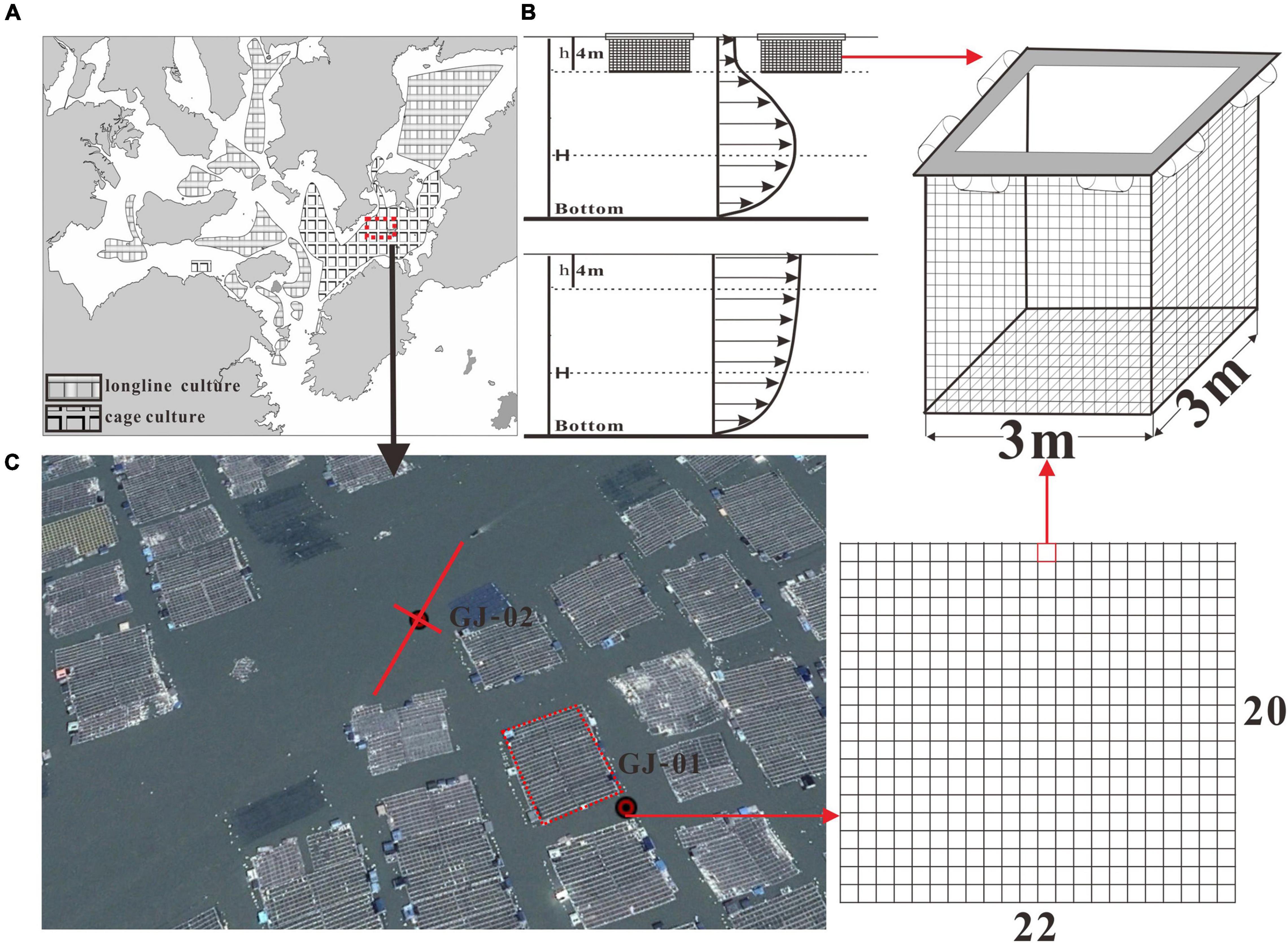
Figure 2. Distribution of longline and cage aquaculture farms in the Sansha Bay based on the Google map digitization (A), a sketch of a single raft cage, and also a conceptual sketch of tidal boundary layer velocity profiles with (upper panel) and without (lower panel) the influence of suspended cages (B), and the distribution of cages around GJ-01 and GJ-02 in the Google map photographed on September 12, 2019. An aquaculture unit around GJ-01 is shown on the right, which consists of 22 × 20 cages (C). The rotated coordinate system is also shown to better represent the real flow direction. The long red line indicates the direction of streamwise component u, whereas the short red line indicates the direction of spanwise component v.
Data Collection
A field campaign was conducted from July 14 to 24, 2019 near Dongan island, where the densest cage aquaculture farms are regularly arranged with a narrow and straight ship channel at the center (Figure 2C). Hydrographic surveys were carried out using a bottom-mounted tripod, a surface floating platform, and the ship-based cast. GJ-01 is located inside the cage aquaculture farm and GJ-02 in the ship channel outside the farm (Figure 2C). The distance between the two stations is about 240 m.
A Flowquest 600 kHz acoustic Doppler Current Profiler (ADCP) and an optical backscatter sensor (OBS) with built-in temperature and salinity sensors (OBS-3A, D&A Instrument Com) were fixed on the surface floating observation platform (Table 1). The ADCP was downward-looking, with a bin size of 0.5 m and a sampling interval of 60 s. The sampling interval of OBS was configured as 60 s. The floating observation platform was first placed at GJ-01 for a continuous observation of 68 h since 17:00 on July 13. Afterward, it was moved to GJ-02 for another continuous observation of 27 h since 13:30 on July 16. Time series of sea surface temperature, salinity, and turbidity and also the variabilities of the current velocity profile at the two stations were obtained.
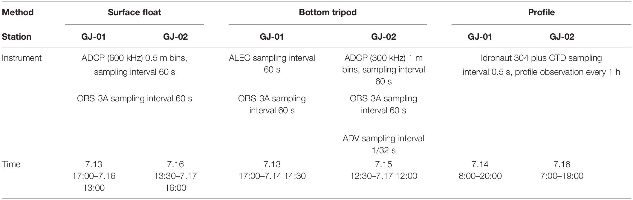
Table 1. Information of the instruments and their deployment and working modes.
The bottom-mounted tripod equipped with an ALEC current meter and an OBS-3A was first deployed at GJ-01 from 17:00 on July 13 to 14:30 on July 14. However, the data of the ALEC current meter were not used because we focused on the flow structures impacted by the farm facilities. The tripod was reset and deployed at GJ-02 from 12:30 on July 15 to 12:00 on July 17. The instruments included OBS-3A, acoustic Doppler velocimeter (ADV, Nortek 6 MHz Vector), and a Flowquest 300 kHz ADCP. The sampling interval of OBS was 60 s; the sampling frequency of ADV was 32 Hz; the sampling interval of ADCP was 60 s; and the vertical bin size was 1 m (Table 1).
Profiling observation was carried out using a CTD with a built-in OBS 3+ sensor (Idronaut 304 plus) at GJ-01 (8:00–20:00, July 14) and GJ-02 (7:00–19:00, July 16). Water samples were collected using a pump from the three different water depths near the surface, the half, and near the bottom. The CTD was configured to sample at a rate of 2 Hz. During the profiling observation, the wind speed and direction were also measured using an anemometer. The wind speed was small during the whole observation period (average wind speed was 1.2 m/s), which indicates to have little impact on the local hydrodynamics.
Data Processing
Current velocities were averaged over 10-min segments and then rotated into a streamwise component u, which is approximately parallel to the shoreline and also roughly parallel to the ship channel (positive u indicates flood current toward ∼60°) and a spanwise component v (positive toward the north shore). The downward-looking 600 kHz ADCP at GJ-01 was placed on the surface float with the transducer locating at ∼ 0.3 m below the sea surface. The available velocity records were determined by blanking zones (0.7 m and 1.4 m for 300 and 600 kHz AD, respectively) adjacent to the transducer and side-lobe effect far from the transducer. Thus, the velocity recorded covers the water column between 1.95 m below the surface and 0.07 h above the bed (h is the water depth). The bottom-mounted 300 kHz ADCP at GJ-02 was deployed at 1.88 m above the bed. The first velocity bin was located at 5.76 m above the bed and the last one at ∼ 0.07 h below the sea surface. The velocity data had been extended to the near-bed region combined with the ADV data (0.75 m above the bed).
Results
Temporal Variations in Water Level, Temperature, and Salinity
Temporal variations in water levels at GJ-01 and GJ-02 are shown in Figure 3A, together with contemporary tidal level change at Bangmen station. It is clearly shown that the Sansha Bay is primarily dominated by the semidiurnal tide. Slight tidal asymmetry was exhibited with the flood and ebb tides lasting for on average 6 and 6.5 h, respectively.
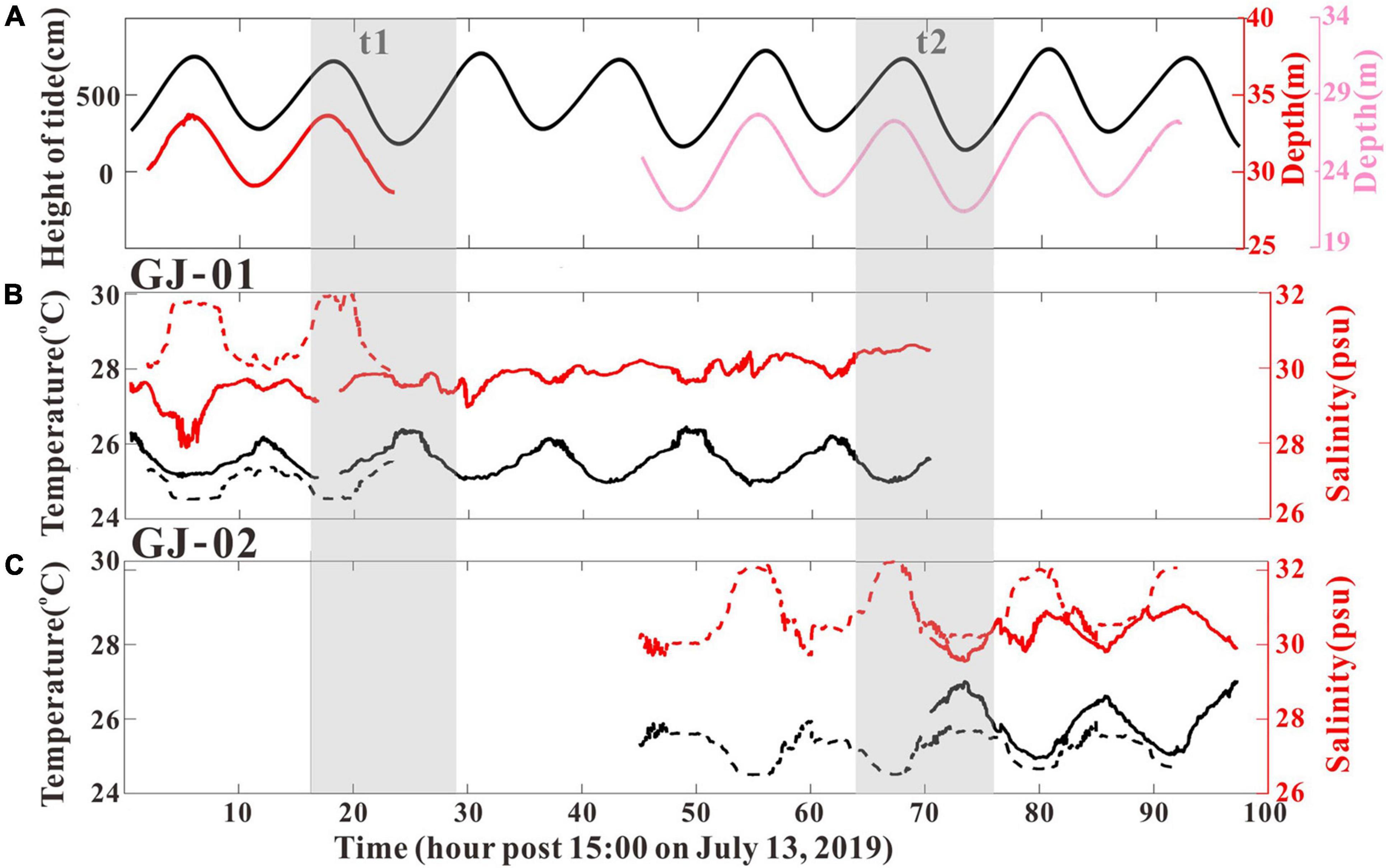
Figure 3. Time series of water-level change at GJ-01 (red line) and GJ-02 (pink line), and also tidal elevation change at Bangmen tide-gauging station (black line) (A), temperature and salinity at GJ-01 (B), and temperature and salinity at GJ-02 (C). Surface (Bottom) water temperature and salinity are indicated by black (black dotted) and red (red dotted) lines, respectively. The two gray-shaded periods (t1, t2) represent the periods of hourly CTD casts at GJ-01 and GJ-02, respectively.
The OBS-3A data from the GJ-01 and GJ-02 are combined to present the local hydrographic characteristics. The water-level time series suggested tide at Bangmen (bay head) lagged ∼ 0.5 h behind the campaigning site (Figure 3A). Both the surface and bottom temperatures were highly modulated by the tide in terms of the presence of high (low) temperature at the ebb (flood) slacks (Figures 3B,C). At GJ-01, surface temperature and salinity were monitored during 0.5–70.5 h, whereas the bottom temperature and salinity were monitored during 0.5–22 h (Figure 3B). At GJ-02, surface temperature and salinity were monitored during 71–96 h, whereas the bottom temperature and salinity were monitored during 45–91 h (Figure 3C). The surface water temperature during 0.5–70.5 h fluctuated between 25.2 and 26.4°C, but the maximum surface water temperature rose up to 27°C during 71–96 h. The bottom water temperature ranged from 24.3°C to 25.5°C, without the presence of relatively higher temperatures during the last 25 h as shown at the surface water temperature.
The surface water salinity varied between 28 and 30 psu during 0.5–70.5 h (Figure 3B). However, the salinity decreased significantly during 2–5 h to the lowest value of 28 psu before a gradually rising pattern. The surface water salinity during 71–96 h reached up to 30–31 psu (Figure 3C). The bottom water salinity during the observation period reached 30–32 psu. The bottom salinity demonstrated remarked semidiurnal tidal signal, but the surface salinity showed higher frequency variations that potentially linked with M4 shallow-water tidal constituent (Figures 3B,C).
The vertical structures of water salinity, temperature, and density anomaly σ (ρ-1000) are presented in Figure 4 during the observational periods of t1 and t2 as indicated in Figure 3. The water temperature variation patterns were quite similar at the two stations, both varying with the tide with the presence of warmer (colder) water at the ebb (flood) slacks. The temperature variations were in the range of 1–3°C over the entire water column. The saline stratification is stronger around the flood slack and collapsed down at the ebb slack. The maximum salinity difference between the surface and the bottom on July 14 at GJ-01 was 3.37 psu which occurs at the end of flood and the minimum was 0.97 psu which occurs at the end of ebb. Similar temporal variations had been observed on July 16 at GJ-02 with a maximum surface–bottom salinity difference of 2.76 psu and a minimum difference of 0.89 psu. The density variation was similar to salinity. The maximum surface–bottom density difference was 3 kg m–3 and the minimum was 1 kg m–3 on July 14, and the maximum surface–bottom density difference was 2 kg m–3 and the minimum was 1 kg m–3 on July 16.
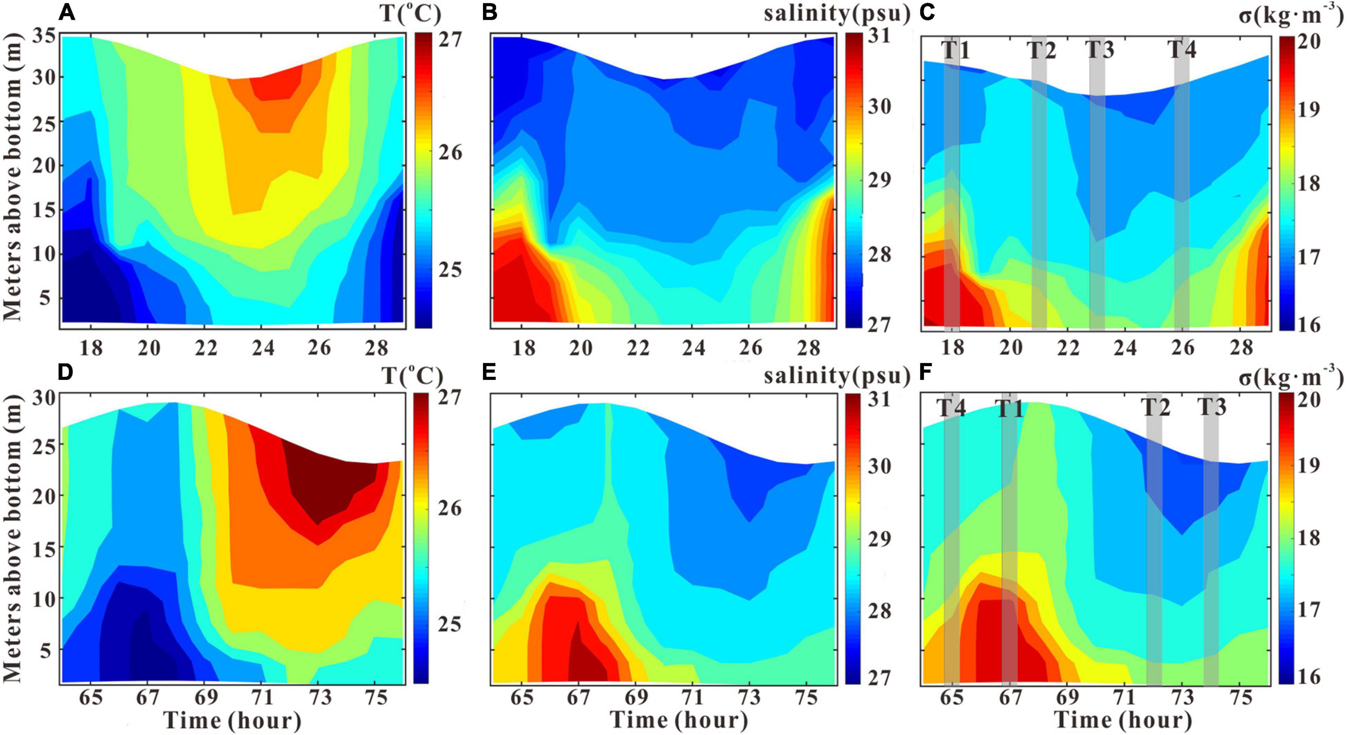
Figure 4. Hourly variations in the vertical structure of temperature, salinity, and density anomaly σ (ρ-1000) at GJ-01 on July 14, 2019 (A–C), and those at GJ-02 on July 16, 2019 (D–F). T1–T4 are the selected periods representing flood slack, maximum ebb, ebb slack, and maximum flood, respectively.
Vertical Structure of Tidal Current
Figure 5 shows temporal variations in vertical structures of flow velocities u and v at the stations GJ-01 and GJ-02. The flood and ebb tides lasted for on average 6 h and 6.5 h, respectively. The peak u of GJ-01 exceeded 1 m/s during the flood tide and that of the ebb tide was 0.97 m/s. The maximum u of GJ-02 was 0.92 m/s during the flood tide and 0.74 m/s during the ebb tide. At GJ-01, the depth-averaged u for the flood and the ebb tides were 0.37 m/s and 0.39 m/s, respectively. The similar u values were observed at GJ-02 with 0.4 m/s and 0.38 m/s for the flood and the ebb tides, respectively. The small values of depth-averaged v at the two stations were almost identical (Table 2). The maximum current velocities occurred during the half of flood (ebb) tide, and the minimum current velocities occurred at flood (ebb) slack. In addition, there was significant lateral circulation at both stations from the vertical characteristics of v (Figures 5B,D). At flood, the upper layer water flowed southwest while the lower layer water flowed northeast, and vice versa during the ebb.
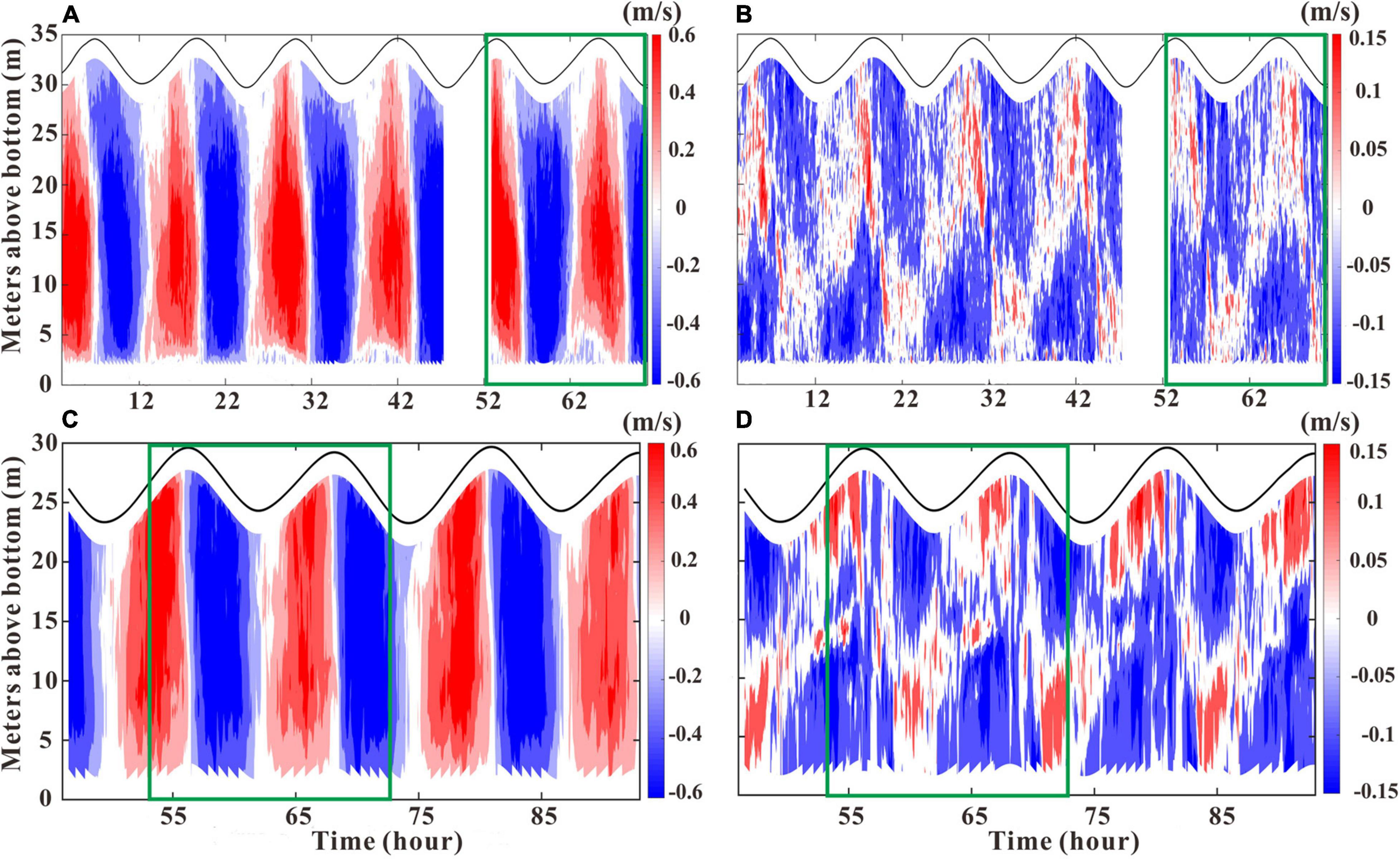
Figure 5. Current velocity profile of u and v at GJ-01 (A,B) and GJ-02 (C,D). The green boxes indicate the current data measured synchronously at the two stations. The current profile of GJ-01 was measured by the downward-looking ADCP 600 kHz on the surface, and the current profile of GJ-02 was measured by the upward-looking ADCP 300 kHz on the tripod.
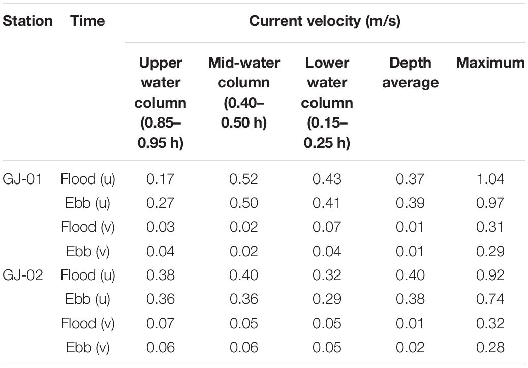
Table 2. Statistics of current velocity at the two stations.
Streamwise and spanwise current velocities at the upper (0.75–0.85 h) (us, vs), the mid (0.4–0.5 h) (um, vm), and the lower (0.15–0.25 h) (ub, vb) water column have been shown in Figure 6. The difference of current velocities (i.e., vertical shear) in different layers was mainly reflected in u (Figures 6A,C), whereas the difference of v was not obvious (Figures 6B,D). The mean absolute values of um and ub at GJ-01 were 0.51 m/s and 0.43 m/s, respectively, whereas it was only 0.24 m/s in the near-surface layer (Figure 6A). The mean absolute ub value at GJ-02 was 0.31 m/s, and the mean absolute values of um and us were identical at 0.38 m/s.
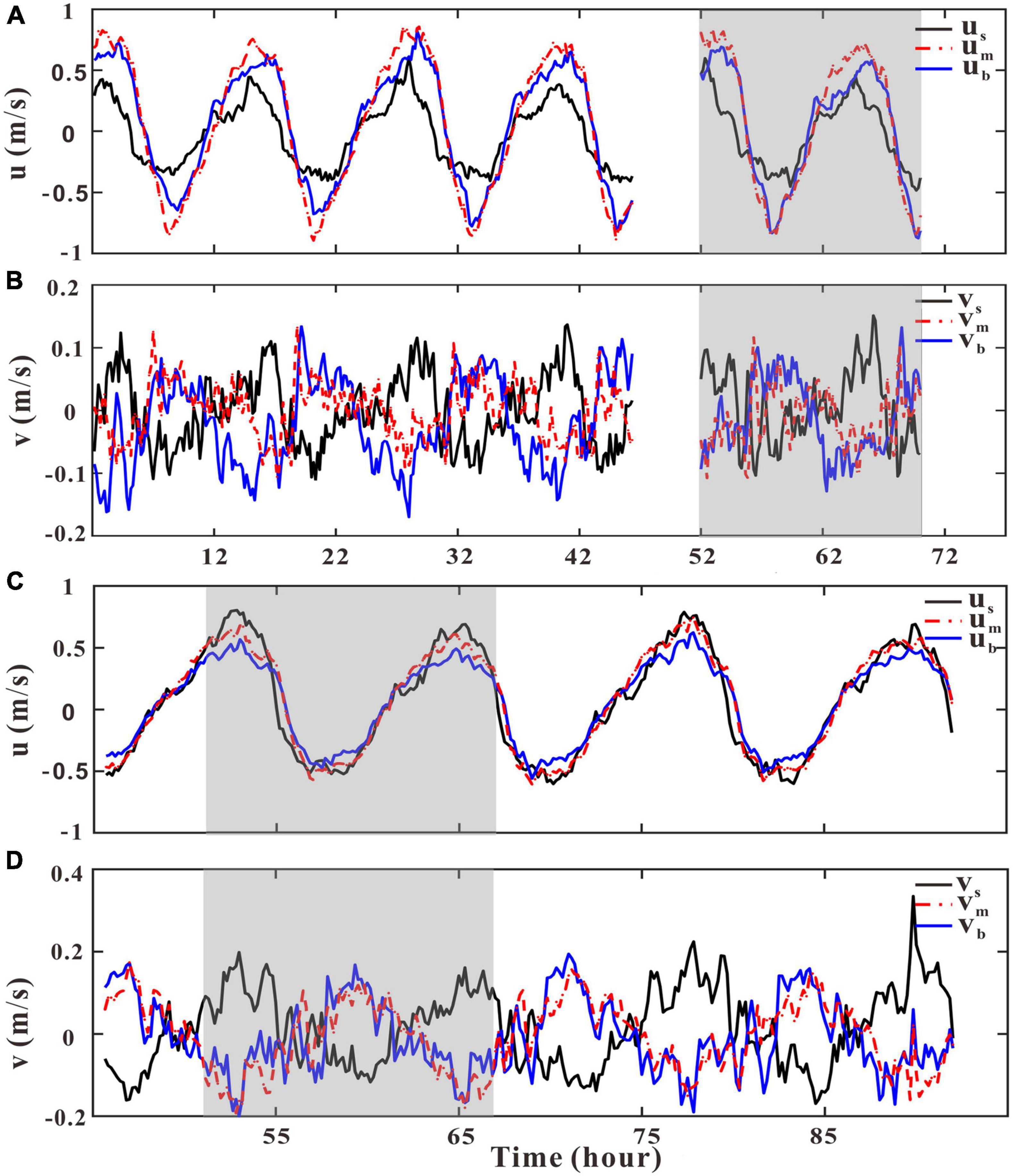
Figure 6. Time series of u and v at the upper (0.75–0.85 h), the lower (0.15–0.25 h), and the mid (0.4–0.5 h) water column at GJ-01 (A,B) and GJ-02 (C,D). The near-surface, mid, and near-bottom current velocities are shown in black, red, and blue, respectively. The shaded parts indicate the current data measured synchronously at the two stations.
Stratification and Mixing
Time series of densities ρ (S, T, p) at the near-surface and near-bottom layers and also their difference are presented in Figure 7. It is clearly seen that the density varies in phase with the tide, that is, elevated density at the high tide and reduced density at the low tide. Periodic density stratification existed at both stations. The stratification gradually increased during the flood tide and reached the maximum at the flood slack. The stratification gradually decreased during the ebb tide and reached the minimum at the ebb slack. The maximum surface–bottom density difference of GJ-01 and GJ-02 was about 3 kg m–3 and 1.5 kg m–3, respectively, whereas the minimum density difference was 0.53 kg m–3 at GJ-01 and was close to 0 at GJ-02.
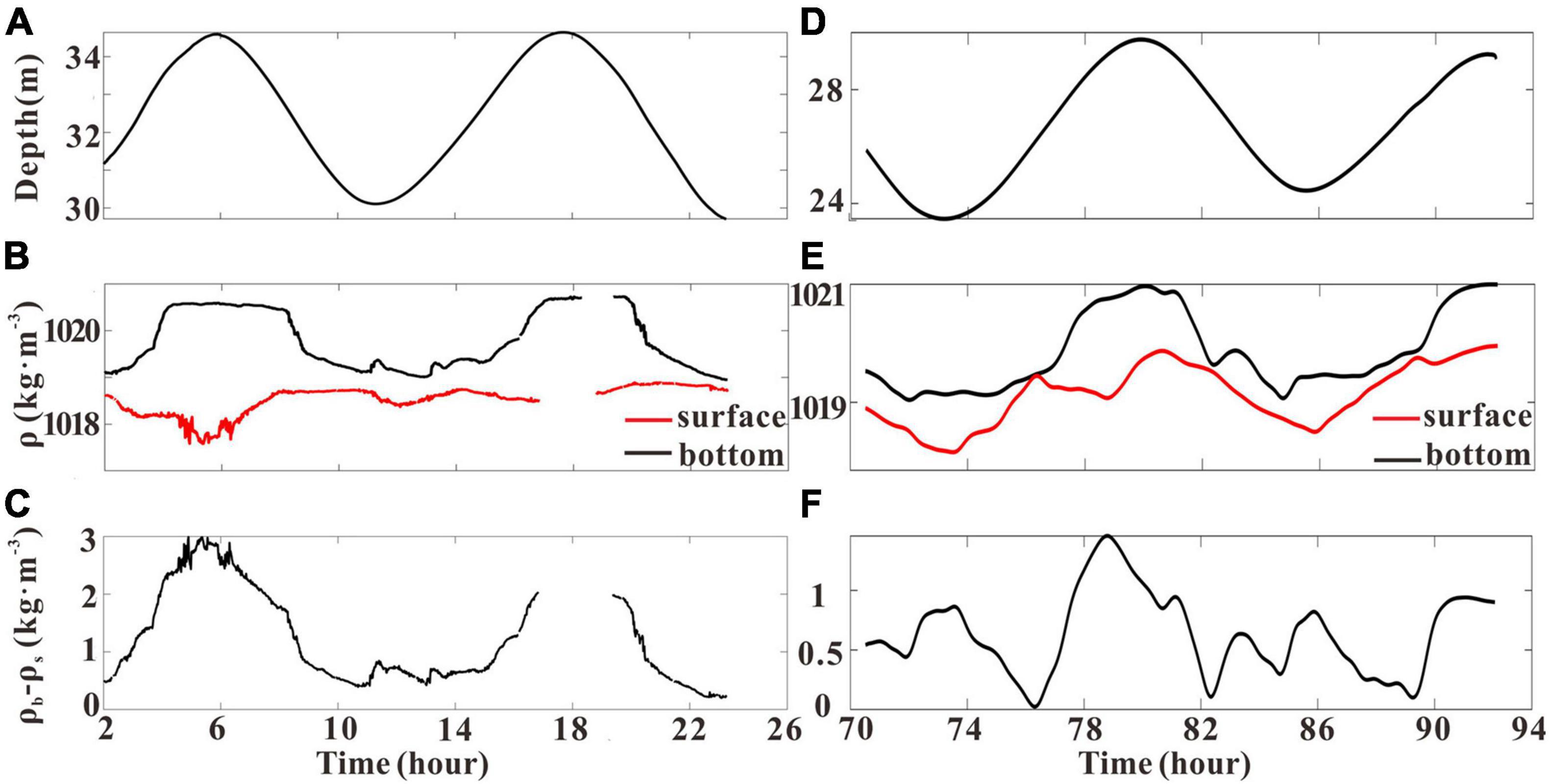
Figure 7. Time series of water depth, surface (red line) and bottom (black line) density, and the surface–bottom density difference at GJ-01 (A–C), and water depth, surface (red line) and bottom (black line) density, and the surface–bottom density difference at GJ-02 (D–F).
The vertical structures of density are presented in Figure 4. There were visible differences between the upper water column and the lower water column at two sites. The density of the upper water column at GJ-01 changed with a small magnitude less than 0.3 kg m–3 over the whole tidal cycle (Figure 4C), which indicates the poor horizontal water exchange within the cage farm. However, the density of the upper water column at GJ-02 varied in a range of more than 1 kg m–3, significantly larger than that of GJ-01 in the tidal cycle (Figures 4C,F). The density variations were quite similar in the lower water column at the two sites with a similar range of 2 kg m–3. The stratification around the high tide was stronger than the low tide.
Discussion
Hydrodynamic Change by the Cage-Induced Drag
As shown in Figure 6 and discussed earlier, the flow velocity at the upper water column has been significantly reduced. As the wind speed measured by anemometer during the whole observation period was very small (average wind speed was 1.2 m/s), the effects of wind stress on the near-surface current are expected to be negligible. Therefore, the streamwise velocity (u) reduction in the upper layer is believed to be mainly due to the existence of cage facilities, whereas the spanwise (v) velocities were almost unaffected. Given that the maximum u generally appeared in the mid-water column at both sites, the near-surface (us) and near-bottom (ub) velocities of GJ-01 and GJ-02 were then fitted with the mid-layer (um) velocities to quantify the cage farm’s influence (Figure 8). The reduction in current velocities due to the canopy and bottom drag can be conveniently characterized by the slope of scatterplots of us vs. um and ub vs. um. As shown in Figure 8C, the us values were almost equal to the um at GJ-02 outside the cage farm. The slope of the scatterplots between us and um at GJ-01 was 0.46 (Figure 8A), which indicates that the near-surface velocities were reduced by 54% due to the cage-induced drag. The slope of the best fit line of the scatterplots between the ub and the um was closest to GJ-01 (0.83) and GJ-02 (0.75; Figures 8B,D), which implies that the cage-induced drag effect should not reach the near-bottom layer.
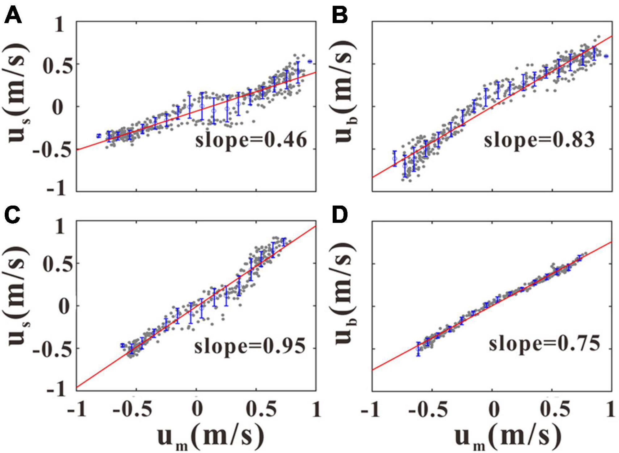
Figure 8. Scatterplots of um vs. us at GJ-01 and GJ-02 (A,C) and um vs. ub at GJ-01 and GJ-02 (B,D). Gray dots indicate 10-min average data of raw streamwise velocities (u) at the three representative layers, and blue circles and error bars represent bin-averaged ub values over an interval of 0.1 m/s along the x-axis and associated standard deviations. The red lines are obtained by the linear fitting of u data shown by gray dots.
We further selected tidal current data measured synchronously during the period from 19:00 on July 15 to 13:00 on July 16 at the two stations to do a comparison for the hydrodynamic response of the cage farm. The results show that the us at GJ-01 was on average only 58% of that at GJ-02 (Figure 9A). The ub at GJ-01 was on average 1.12 times that of GJ-02 (Figure 9B), and also indicates that the near-bottom layer was hardly affected by the cage-induced drag. The depth-averaged current velocities inside and outside the cage farm were almost identical (Figure 9C). Given the small distance between the two sites, the highly reduced us at GJ-01 was most likely due to the friction induced by the aquaculture facilities. Based on field observations in winter, Lin et al. (2019) narrated that the surface current velocities were reduced by 70% in the deep tidal channels and 50% on the tidal flats due to the friction induced by the aquaculture facilities in the Sansha Bay. The surface current velocities were reported to decrease by 40% in the raft kelp aquaculture farm in Sanggou Bay, China (Shi et al., 2011) and decrease by 75–90% in the longline mussel aquaculture farm in Zhoushan, China (Lin et al., 2016). Plew et al. (2005) found that the surface current velocities decreased by 36–63% in the raft mussel aquaculture farm in Golden Bay, New Zealand.
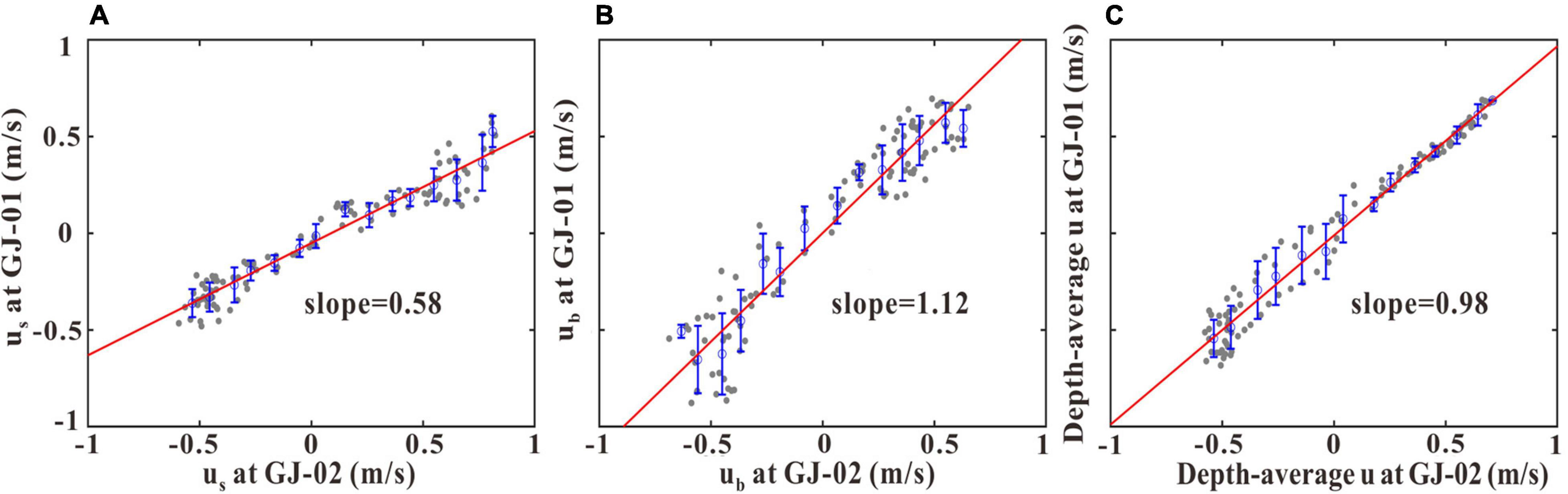
Figure 9. Scatterplots of us (A), ub (B), and the depth-averaged u (C) of GJ-01 vs. GJ-02. The symbols are identical to those in Figure 8.
The difference in the reduction magnitudes of surface current velocities could be influenced by different aquaculture types and densities in different farms. Using a three-dimensional numerical model, Zhao et al. (2013a) found that plane-net inclination angle, height, number, and the spacing distance between two plane nets can reduce the flow velocity downstream to different extents. Based on their numerical modeling results, Zhao et al. (2013b) found the flow reduction increases with increasing cage number. Zhao et al. (2015) conducted a series of physical model experiments and argued that the net cages arranged in double columns have less flow reduction inside the cage than the single column cage arrangement. On the other hand, the flow might cause the deformation of the flexible cage net, which amplifies the blockage effect on the flow (Bi et al., 2014b). When water flows through a net cage, which acts as an obstacle, a wake is formed downstream. This shielding effect can cause significant flow velocity reduction. As shown in experimental data and confirmed by numerical results, Bi et al. (2014a) found greater shielding effects with more cage nets. The flow velocity reduction may also be influenced by biofouling. The accumulation of biofouling attached to the net cages can increase the drag force, which will further aggravate the reduction in flow velocity (Bi et al., 2018, 2020). Bi et al. (2018) observed a maximum flow attenuation of 21.4% which is caused by biofouling based on the observations and laboratory experiments, and the drag acting on the net increases with increasing level of biofouling.
To summarize, we observed that the flow velocities and the water momentum passing through the cage are reduced within the cage due to the obstruction of cage aquaculture facilities. A tidal surface boundary layer is well-formed due to the frictional effects induced by suspended aquaculture as surface obstruction (Fan et al., 2009). The flow velocities are reduced due to the friction of the cage below the cage, and the flow velocities gradually recover downward from the cage. Moreover, due to the viscosity of the fluid, the recovery of flow velocity needs a certain process. Plew (2011b) divided the velocity profile into a bottom boundary layer, a canopy shear layer (i.e., a boundary layer caused by the structure), and an internal canopy. Velocity is reduced both in the canopy-induced shear layer and in the bottom boundary layer (Lin et al., 2016; Liu and Huguenard, 2020). The thickness of the shear layer is related to the canopy-induced drag and the distance between the canopy and the bottom boundary layer (Plew, 2011b). At the same bay with the same cage aquaculture facilities, Lin et al. (2019) reported that the cage-induced drag on the flow field can reach as deep as greater than 10 m in relatively deep channels of the Sansha Bay.
The range of the flow reduction effects might also be related to structural parameters of the cage net, such as the solidity ratio. According to Tang et al. (2017), the solidity ratio (α) can be calculated as , where d is the twine diameter, l is the bar length, and φ is the opening angle (Tang et al., 2017). In this study, l = 32.8 mm, d = 5.6 mm, but φ is hard to measure in the field as it might vary as the oscillating tidal flow. Assuming a constant φ = 45° that is used in flume tests of Tang et al. (2017), we obtain a rough estimate of α = 0.31. However, an accurate calculation of this parameter is not possible using our present dataset and thus requires more observational data in the future research. The present observation data aim to investigate the impact of cage aquaculture on large-scale hydrodynamic forces, and the influence of some detailed parameters, such as the consolidation ratio and the biological fouling on hydrodynamic forces, is not a focus of our current observations.
The vertical structures of u at GJ-01 (u1) and GJ-02 (u2) are investigated how deep the cage-induced friction can influence during the selected flood and ebb tides (Figure 10A). The cage-induced drag is clearly seen in the u profiles at GJ-01, where the u values decreased rapidly upward from the maximum ebb velocity at z/h≈0.25 (Figure 10B), and the maximum flood velocity at z/h≈0.4 (Figure 10E). The downward decreased u values at the lower water column at GJ-01 were due to bottom friction as those were also shown at the bottom boundary layer of GJ-02 (Figures 10C,F). However, the surface boundary layer induced by the friction of cage farms at GJ-01 was not observed at GJ-02 where the u values changed slightly upward in the upper-mid water column (Figures 10C,F). It is therefore implied that the cage-induced drag on the flow field can reach down to z/h = 0.25. The ratio of mean u squared at GJ-02 against GJ-01 shows generally upward-increasing patterns with the visible difference between the flood and the ebb tides (Figures 10D,G). The causes for such differences need further investigations.
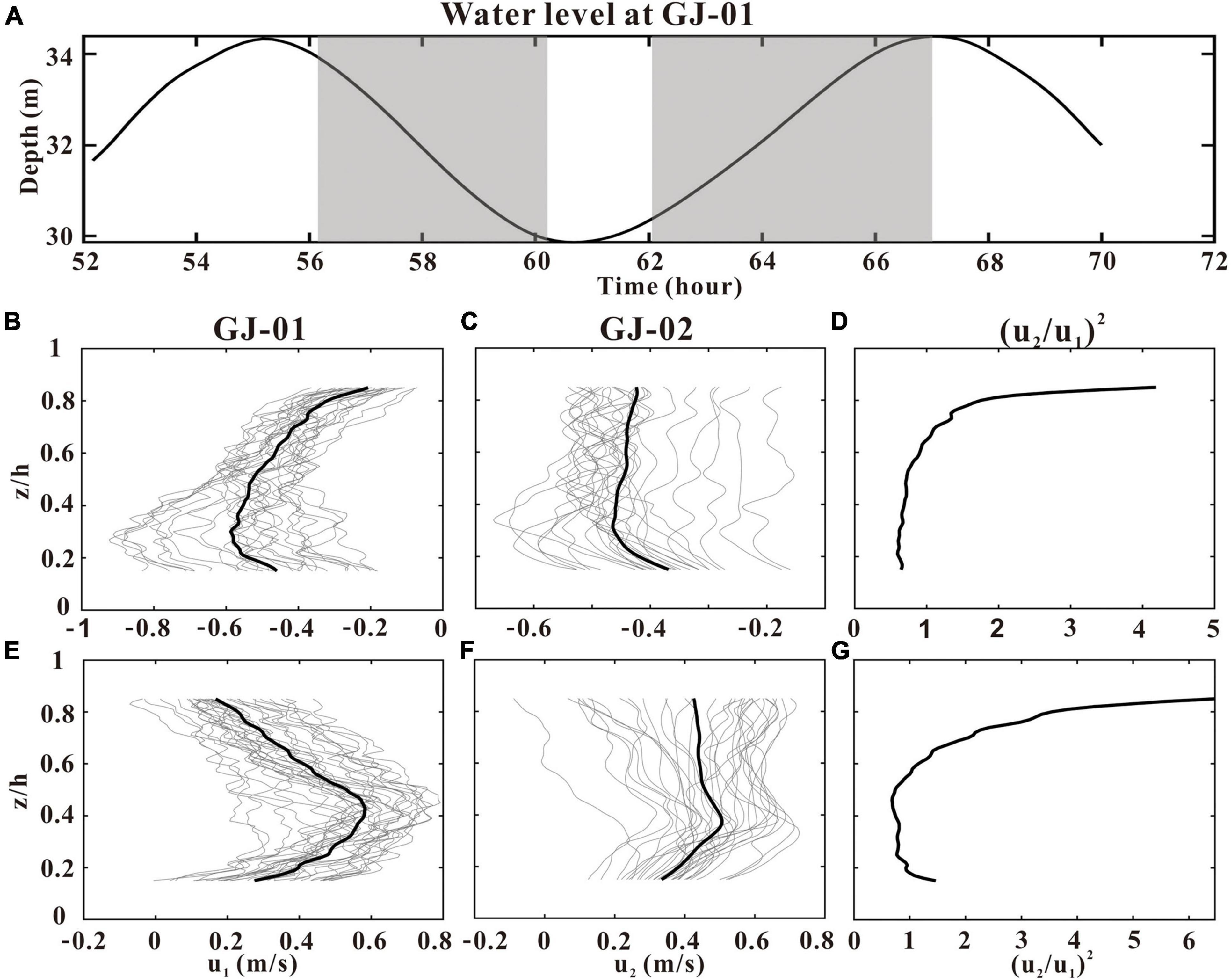
Figure 10. Profiles of u at GJ-01 (u1) and GJ-02 (u2) during the ebb (B,C) and flood tides (E,F). Water-level variations at GJ-01 were plotted in panel (A) with the two selected periods (in gray) when the absolute depth-averaged u was larger than 0.2 m/s. The gray and black curves in panels (B,C,E,F) were plotted using the 10-min average u data and the average u data over the two selected periods. The ratio of u squared at GJ-02 and GJ-01 was plotted in panels (D,G). z is the height above the bed, and h is the water depth.
Potential Mechanisms Influencing Stratification and Mixing
Periodic Stratification and Lateral Circulation
As shown in section “Stratification and Mixing,” periodic stratifications were observed at both stations. Stratification increased during the flood tide, reached the maximum at the high tide, then decreased during the ebb tide, and approached a well-mixed state at the low tide. Because this phenomenon existed in both stations, we believe that the periodic stratification is not directly related to the presence of cage farms. It is worth noting that the periodic stratification as observed here is opposite to that caused by classic tidal straining. The latter tends to favor the development of stratification during the ebb tide and the destruction of stratification during the flood tide (Simpson et al., 1990). Thus, another mechanism must be responsible for the stratification generation in this study.
Lateral circulation basically represents a horizontal circulation in the horizontal direction perpendicular to the main channel. Because it is a circulation, a vertical fluid motion should be inherently involved. In this case, the effect of horizontal flow is major, and the vertical motion is minor. The periodic stratification observed in the Wadden Sea (Becherer et al., 2015) is consistent with our observations. They found that the periodic stratification was mainly controlled by the balance between the strong transverse pressure gradient force generated by lateral circulation and turbulence, whereas the longitudinal tidal straining was very small and could be almost ignored. Lacy et al. (2003) and Scully and Geyer (2012) observed the same phenomenon in estuaries with lateral circulation. In this study, lateral circulation existed at the two sites from the profiles of spanwise current velocity (v) (Figures 5B,D). In addition, the intratidal variations in vertical stratification were in phase with temporal variations in lateral circulation. Therefore, we believe that the stratification may be mainly associated with the observed lateral circulation. Besides, the poor water exchange capacity of the upper water column at GJ-01 hindered the entry of saltier seawater as shown by the small salinity and density variation ranges (Figures 4B,C), which further increased the density difference between the surface and the bottom layers at the high tide. Unfortunately, this hypothesis cannot be justified using our present dataset because the lateral density gradient cannot be estimated; thus, further observational direct evidences are still expected.
Enhanced Vertical Mixing by Cage Farms
The stability of a stratified shear flow can be assessed through the gradient Richardson number Rig (Bowden, 1963),
The gradient Richardson number is the ratio of the strength of the density stratification to the strength of the current shear. The primary measure of strength of stratification is the buoyancy frequency squared N2 (Brunt, 1927),
where g is gravitational acceleration, ρ0 is a reference density, and the z is the height above the bed. The velocity shear is calculated from
At high values of Rig, the stabilizing effect of the density gradient dampens turbulence, reducing vertical mixing. It is generally thought that stratified shear flows are stable if Rig > 0.25 everywhere in the flow (Turner, 1973). Rig was estimated based on the ADCP velocity records and the hourly profiling CTD data.
We selected several typical periods (T1–T4, Figure 4) to investigate the impact of aquaculture structures on vertical mixing (Figures 11, 12). Although the density stratification existed at both stations (Figure 7), their flow stability patterns were different (Figures 11, 12). Stable stratification (Rig > 0.25) existed at GJ-02 except the near-bottom layer (Figure 11), and the square of velocity shear in the subsurface layer (5–10 m below the sea surface) was close to 10–4 s–2. However, the subsurface layer of GJ-01 (shaded part of Figure 12) was well-mixed (Rig < 0.25). The square of velocity shear of GJ-01 was in the order of 10–3 s–2, which indicates that the velocity of the subsurface water body was strongly sheared, enhancing vertical mixing. The stable stratification (Rig > 0.25) was mainly in the mid-water column (20–25 m below the sea surface). In the stable region, the current velocities were large and current shears were weak, suggesting a regime affected neither by the cage-induced nor by the bed-induced drag. Velocity shear caused by the friction enhanced the local mixing in the near-surface and the near-bottom layers, corresponding to the “double-drag layers” observed in the current speed profiles (Figures 5A, 10B,E).
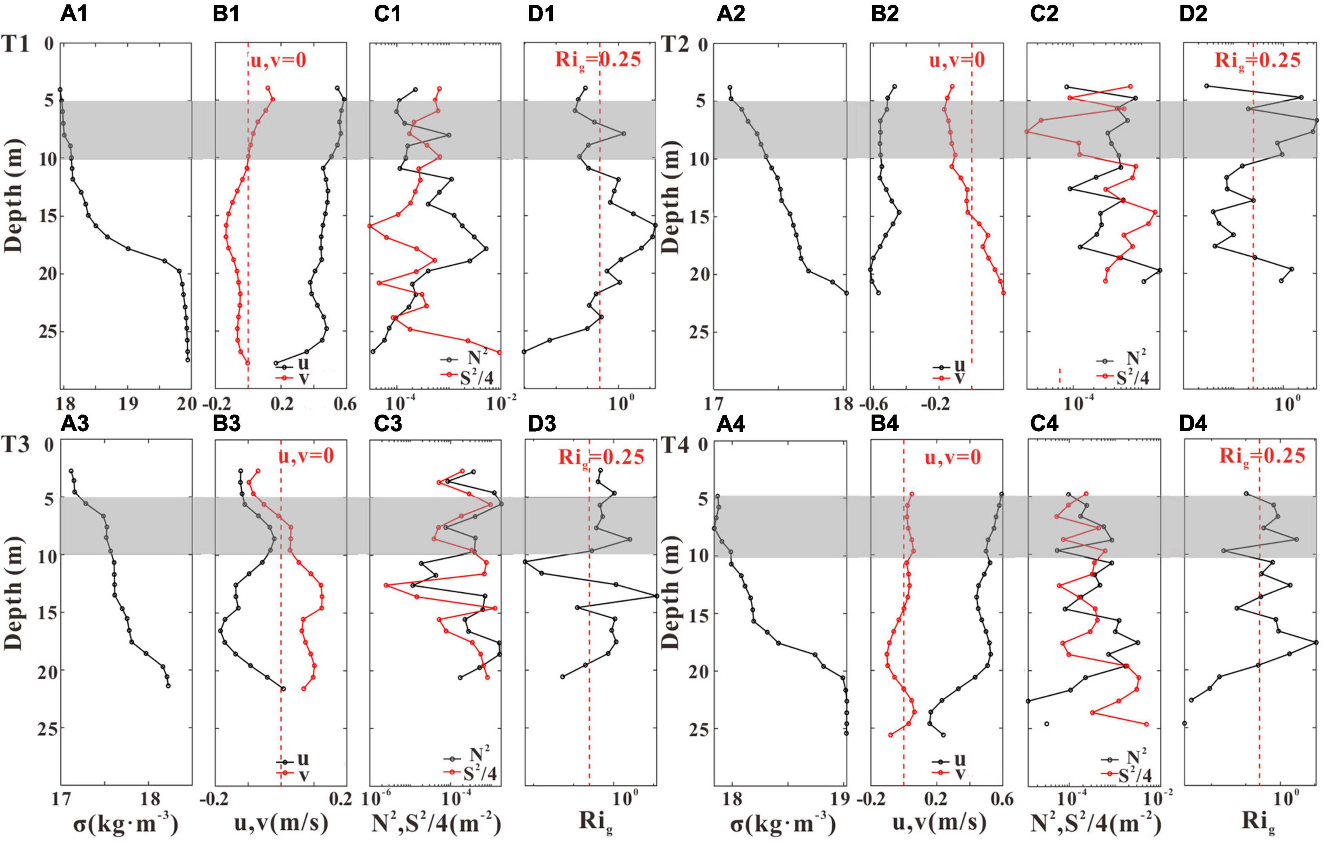
Figure 11. The profiles of density anomaly σ (A1–A4), u (black line) and v (red line) (B1–B4), the square of buoyancy frequency N2 (black line) and the square of velocity shear S2/4 (red line) (C1–C4), and the gradient Richardson number Rig (D1–D4) during the four representative periods T1–T4 at GJ-02. The red dashed lines indicate u (v) = 0 in panels (B1–B4), and Rig = 0.25 in panels (D1–D4), respectively. The shaded parts represent the subsurface (5–10 m) layers.
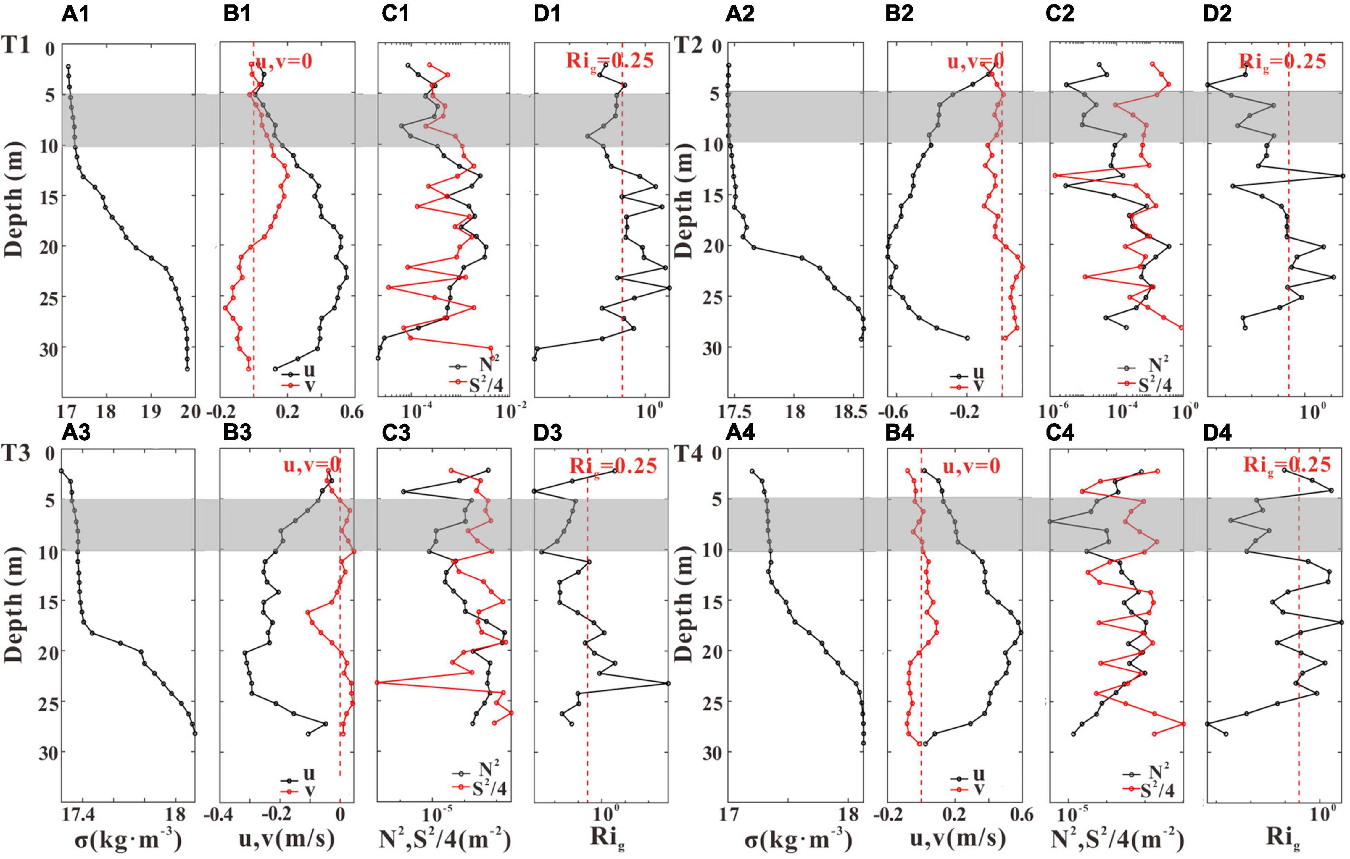
Figure 12. The profiles of density anomaly σ (A1–A4), u (black line) and v (red line) (B1–B4), the square of buoyancy frequency N2 (black line) and the square of velocity shear S2/4 (red line) (C1–C4), and the gradient Richardson number Rig (D1–D4) during the four representative periods T1–T4 at GJ-01. The red dashed lines indicate u (v) = 0 in panels (B1–B4), and Rig = 0.25 in panels (D1–D4), respectively. The shaded parts represent the subsurface (5–10 m) layers.
Liu and Huguenard (2020) reported a similar periodic stratification pattern in the oyster aquaculture farm of Damariscotta River with lateral circulation. They found that during the flood tide, farm-induced drag enhanced the lateral straining of velocity shear to enhance vertical mixing near the surface, but during the ebb tide, the decreased velocity shear due to the reduced surface velocities was difficult to overcome the stratification. Plew et al. (2006) found that the dissipation rate inside the canopy was generally higher than that near the bed, and they both varied with the tide with higher dissipation occurring at faster current speed. Plew (2011b) divided the vertical profiles of velocity into a bottom boundary layer, a canopy shear layer, and an internal canopy layer. The impact of aquaculture activities on vertical mixing and stratification may be related to the cage-induced drag. In our study, the current velocities of the subsurface layer were large during the flood and the ebb tides, and a strong velocity shear could be generated at the cage interface to enhance the local vertical mixing. Therefore, we believe that the well-mixed subsurface layer of GJ-01 may be due to the cage-induced drag, which enhances the shear of current velocity and produces local turbulence, resulting in the vertical mixing. However, due to the lack of high-frequency current velocity data of the near-surface, we are not able to verify whether there is local turbulence in the subsurface layer of GJ-01.
The gradient Richardson number at each 13-h period at the two sites was counted using individual hourly-observation profiles. Figure 13 shows that at the upper water column, 40% of the data at GJ-02 had Rig > 0.25, whereas this percentage dropped to 20% at GJ-01. This indicates that the vertical mixing in the upper water column is stronger within the cage farm than the outside. This indicates the existence of cage farms may enhance the mixing of subsurface layer water. At the mid-lower water column, the Rig of the two stations was not statistically different. Near the bed, Rig decreased due to the enhanced mixing induced by the bottom friction. The 40% of time having Rig > 0.25 in the subsurface layer at GJ-02 was about two times that of GJ-01 (20%). The current shear of the subsurface layer at GJ-01 (10–3 m–2) was about 10 times higher than that of GJ-01 (Figures 11, 12). Therefore, the well-mixed pattern of the subsurface layer inside the cage farm (GJ-01) may be due to the velocity shear caused by the cage-induced drag, resulting in local turbulence to strengthen the vertical mixing. But the specific mechanism of local turbulence is still a challenging problem and needs further investigations.
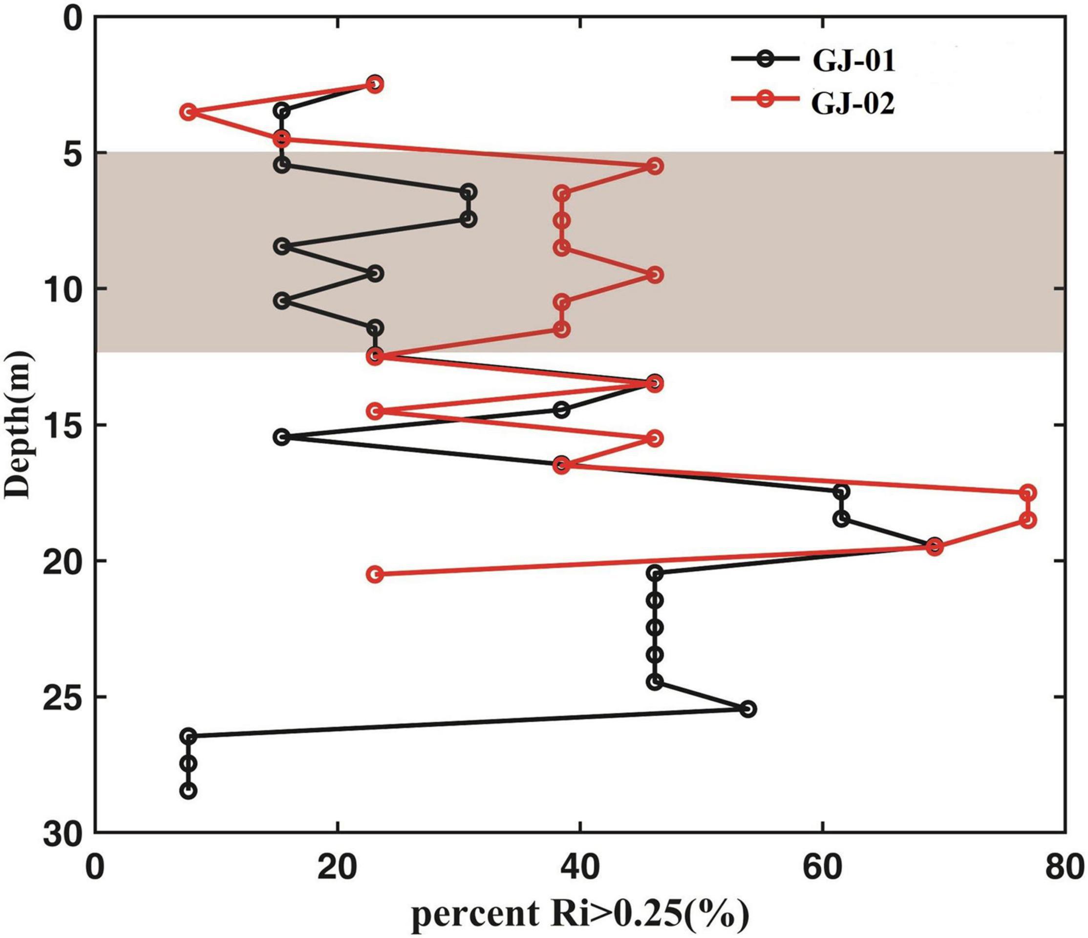
Figure 13. The proportion of the time having Rig > 0.25 is plotted vs. the water depth for GJ-01 (black line) and GJ-02 (red line). The statistics are obtained according to individual hourly-observation profiles.
Conclusion
The influence of cage farms on the flow structures and vertical stratification and mixing in the Sansha Bay was investigated based on observational data. The results indicated that the current velocities were relatively uniform in the vertical in the cage-free channels, where a single bottom boundary layer was developed without the surface boundary layer. However, a surface boundary layer was well-formed due to the frictional effects inducted by extensive, high-density cage facilities as the surface obstruction, resulting in the vertical “double-drag layers” structure. More specifically, the surface friction induced by the cage facilities caused current velocities to reduce by 54% in the upper layer and only 17% in the near-bottom layer. The cage-induced drag decreased with the increasing depth, reaching 3/4 of the water column from the surface. The decrease in current velocities reduced the horizontal exchange capacity of the upper water column, where the salinity inside the cage farm was low over the whole tidal cycle with a small density variation less than 0.3 kg m–3.
Periodic stratification phenomena were influenced by lateral circulation in the bay. The stratification of the two stations increased during the flood tide and decreased during the ebb tide. However, the subsurface layer (5–10 m below the sea surface) inside the cage farm was well-mixed through studying the gradient Richardson number (Rig). The 40% of time having Rig > 0.25 in the subsurface layer outside the cage farm was about two times that inside the cage farm (20%). The current shear of the subsurface layer inside the cage farm (10–3 m–2) was about 10 times higher than that outside the cage farm. Therefore, enhanced velocity shear by the cage-induced drag produced local turbulence to strengthen vertical mixing of the subsurface layer inside the cage farm.
Data Availability Statement
The original contributions presented in the study are included in the article/Supplementary Material, further inquiries can be directed to the corresponding author/s.
Author Contributions
XJ collected and analyzed the data and wrote the manuscript. JT designed the experiments, collected and analyzed the data, and revised the manuscript. DF conceived the idea, designed the experiments, analyzed the data, and revised the manuscript. All authors contributed to the article and approved the submitted version.
Funding
This study is supported by the National Natural Science Foundation of China (41976070 and 41906052).
Conflict of Interest
The authors declare that the research was conducted in the absence of any commercial or financial relationships that could be construed as a potential conflict of interest.
Publisher’s Note
All claims expressed in this article are solely those of the authors and do not necessarily represent those of their affiliated organizations, or those of the publisher, the editors and the reviewers. Any product that may be evaluated in this article, or claim that may be made by its manufacturer, is not guaranteed or endorsed by the publisher.
Supplementary Material
The Supplementary Material for this article can be found online at: https://www.frontiersin.org/articles/10.3389/fmars.2021.779866/full#supplementary-material
References
Becherer, J., Stacey, M. T., Umlauf, L., and Burchard, H. (2015). Lateral circulation generates flood tide stratification and estuarine exchange flow in a curved tidal inlet. J. Phys. Oceanogr. 45, 638–656. doi: 10.1175/JPO-D-14-0001.1
Bi, C. W., Chen, Q. P., Zhao, Y. P., Su, H., and Wang, X. Y. (2020). Experimental investigation on the hydrodynamic performance of plane nets fouled by hydroids in waves. Ocean Eng. 213:107839. doi: 10.1016/j.oceaneng.2020.107839
Bi, C. W., Zhao, Y. P., Dong, G. H., Wu, Z. M., Zhang, Y., and Xu, T. J. (2018). Drag on and flow through the hydroid-fouled nets in currents. Ocean Eng. 161, 195–204. doi: 10.1016/j.oceaneng.2018.05.005
Bi, C. W., Zhao, Y. P., Dong, G. H., Xu, T. J., and Gui, F. K. (2017). Numerical study on wave attenuation inside and around a square array of biofouled net cages. Aquac. Eng. 78, 180–189. doi: 10.1016/j.aquaeng.2017.07.006
Bi, C. W., Zhao, Y. P., Dong, G. H., Xu, T. J., and Gui, F. K. (2014a). Numerical simulation of the interaction between flow and flexible nets. J. Fluids Struct. 45, 180–201. doi: 10.1016/j.jfluidstructs.2013.11.015
Bi, C. W., Zhao, Y. P., Dong, G. H., Zheng, Y. N., and Gui, F. K. (2014b). A numerical analysis on the hydrodynamic characteristics of net cages using coupled fluid–structure interaction model. Aquac. Eng. 59, 1–12. doi: 10.1016/j.aquaeng.2014.01.002
Brunt, D. (1927). An investigation of periodicities in rainfall pressure and temperature at certain European stations. Q. J. R. Meteorol. Soc. 53, 1–30. doi: 10.1002/qj.49705322102
Cabre, L. M., Hosegood, P., Attrill, M. J., Bridger, D., and Sheehan, E. V. (2021). Offshore longline mussel farms: a review of oceanographic and ecological interactions to inform future research needs, policy and management. Rev. Aquac. 13, 1864–1887. doi: 10.1111/rap.12549
Fan, X., Wei, H., Yuan, Y., and Zhao, L. (2009). Vertical structure of tidal current in a typically coastal raft-culture area. Cont. Shelf Res. 29, 2345–2357. doi: 10.1016/j.csr.2009.10.007
Ferreira, J. G., Saurel, C., Lencart e Silva, J. D., Nunes, J. P., and Vazquez, F. (2014). Modelling of interactions between inshore and offshore aquaculture. Aquaculture 426–427, 154–164. doi: 10.1016/j.aquaculture.2014.01.030
Food and Agriculture Organization [FAO] (2018). The State of World Fisheries and Aquaculture 2018. Rome: FAO.
Herrera, J., Cornejo, P., Sepúlveda, H. H., Artal, O., and Quiñones, R. A. (2018). A novel approach to assess the hydrodynamic effects of a salmon farm in a Patagonian channel: coupling between regional ocean modeling and high resolution les simulation. Aquaculture 495, 115–129. doi: 10.1016/j.aquaculture.2018.05.003
Holmer, M., Marbá, N., Terrados, J., Duarte, C. M., and Fortes, M. D. (2002). Impacts of milkfish aquaculture on carbon and nutrient fluxes in the Bolinao area, Philippines. Mar. Pollut. Bull. 44, 685–696. doi: 10.1016/S0025-326X(02)00048-6
Huguenard, K. D., Valle-Levinson, A., Li, M., Chant, R. J., and Souza, A. J. (2015). Linkage between lateral circulation and near-surface vertical mixing in a coastal plain estuary. J. Geophys. Res. 120, 4048–4067. doi: 10.1002/2014JC010679
Lacy, J. R., Stacey, M. T., Burau, J. R., and Monismith, S. G. (2003). Interaction of lateral baroclinic forcing and turbulence in an estuary. J. Geophys. Res. 108:3089. doi: 10.1029/2002JC001392
Leary, P. R., Woodson, C. B., Squibb, M. E., Denny, M. W., Monismith, S. G., and Micheli, F. (2017). “Internal tide pools” prolong kelp forest hypoxic events. Limnol. Oceanogr. 62, 2864–2878. doi: 10.1002/lno.10716
Lin, H., Chen, Z., Hu, J., Cucco, A., Sun, Z., Chen, X., et al. (2019). Impact of cage aquaculture on water exchange in Sansha Bay. Cont. Shelf Res. 188:103963. doi: 10.1016/j.csr.2019.103963
Lin, H., Hu, J., Zhu, J., Cheng, P., Chen, Z., Sun, Z., et al. (2017). Tide- and wind-driven variability of water level in Sansha Bay, Fujian, China. Front. Earth Sci. 11, 332–346. doi: 10.1007/s11707-016-0588-x
Lin, J., Li, C., and Zhang, S. (2016). Hydrodynamic effect of a large offshore mussel suspended aquaculture farm. Aquaculture 451, 147–155. doi: 10.1016/j.aquaculture.2015.08.039
Liu, Z., and Huguenard, K. (2020). Hydrodynamic response of a floating aquaculture farm in a low inflow estuary. J. Geophys. Res. 125:e2019JC015625. doi: 10.1029/2019JC015625
Naylor, R. L., Goldburg, R. J., Primavera, J. H., Kautsky, N., Beveridge, M. C. M., Clay, J., et al. (2000). Effect of aquaculture on world fish supplies. Nature 405, 1017–1024. doi: 10.1038/35016500
Newton, A., Harff, J., and You, Z. J. (2016). Sustainability of future coasts and estuaries: a synthesis. Estuar. Coast. Shelf Sci. 183, 271–274. doi: 10.1016/j.ecss.2016.11.017
O’Donncha, F., James, S. C., and Ragnoli, E. (2017). Modelling study of the effects of suspended aquaculture installations on tidal stream generation in Cobscook Bay. Renew. Energ. 102, 65–76. doi: 10.1016/j.renene.2016.10.024
Ottinger, M., Clauss, K., and Kuenzer, C. (2016). Aquaculture: relevance, distribution, impacts and spatial assessments–a review. Ocean Coast. Manag. 119, 244–266. doi: 10.1016/j.ocecoaman.2015.10.015
Pilditch, C. A., Grant, J., and Bryan, K. R. (2001). Seston supply to scallops (Placopecten magellanicus) in suspended culture. Can. J. Fish. Aquat. Sci. 58, 241–253. doi: 10.1139/f00-242
Plew, D. R. (2011a). Depth-averaged drag coefficient for modeling flow through suspended canopies. J. Hydraulic Eng. 137, 234–247. doi: 10.1061/(ASCE)HY.1943-7900.0000300
Plew, D. R. (2011b). Shellfish farm-induced changes to tidal circulation in an embayment, and implications for seston depletion. Aquac. Environ. Interact. 1, 201–214. doi: 10.3354/aei00020
Plew, D. R., Spigel, R. H., Stevens, C. L., Nokes, R. I., and Davidson, M. J. (2006). Stratified flow interactions with a suspended canopy. Environ. Fluid Mech. 6, 519–539. doi: 10.1007/s10652-006-9008-1
Plew, D. R., Stevens, C. L., Spigel, R. H., and Hartstein, N. D. (2005). Hydrodynamic implications of large offshore mussel farms. IEEE J. Ocean. Eng. 30, 95–108. doi: 10.1109/JOE.2004.841387
Rosman, J. H., Koseff, J. R., Monismith, S. G., and Grover, J. (2007). A field investigation into the effects of a kelp forest (Macrocystis pyrifera) on coastal hydrodynamics and transport. J. Geophys. Res. 112:C02016. doi: 10.1029/2005JC003430
Scully, M. E., and Geyer, W. R. (2012). The role of advection, straining, and mixing on the tidal variability of estuarine stratification. J. Phys. Oceanogr. 42, 855–868. doi: 10.1175/JPO-D-10-05010.1
Shi, J., Wei, H., Zhao, L., Yuan, Y., Fang, J., and Zhang, J. (2011). A physical-biological coupled aquaculture model for a suspended aquaculture area of China. Aquaculture 318, 412–424. doi: 10.1016/j.aquaculture.2011.05.048
Simpson, J. H., Brown, J., Matthews, J., and Allen, G. (1990). Tidal straining, density currents, and stirring in the control of estuarine stratification. Estuaries 13, 125–132. doi: 10.2307/1351581
Stevens, C. L., and Petersen, J. K. (2011). Turbulent, stratified flow through a suspended shellfish canopy: implications for mussel farm design. Aquac. Environ. Interact. 2, 87–104. doi: 10.3354/aei00033
Sun, P., Yu, G., Chen, Z., Hu, J., Liu, G., and Xu, D. (2015). Diagnostic model construction and example analysis of habitat degradation in enclosed bay: III. Sansha Bay habitat restoration strategy. Chin. J. Ocean. Limnol. 33, 477–489. doi: 10.1007/s00343-015-4169-8
Tang, H., Hu, F., Xu, L., Dong, S., Zhou, C., and Wang, H. F. (2017). The effect of netting solidity ratio and inclined angle on the hydrodynamic characteristics of knotless polyethylene netting. J. Ocean Univ. China 16, 814–822. doi: 10.1007/s11802-017-3227-6
Tu, J., Fan, D., Zhang, Y., and Voulgaris, G. (2019). Turbulence, sediment induced stratification, and mixing under macrotidal estuarine conditions (Qiantang Estuary, China). J. Geophys. Res. 124, 4058–4077. doi: 10.1029/2018JC014281
Visch, W., Kononets, M., Hall, P. O. J., Nylund, G. M., and Pavia, H. (2020). Environmental impact of kelp (Saccharina latissima) aquaculture. Mar. Pollut. Bull. 155:110962. doi: 10.1016/j.marpolbul.2020.110962
Wang, B., Cao, L., Micheli, F., Naylor, R. L., and Fringer, O. B. (2018). The effects of intensive aquaculture on nutrient residence time and transport in a coastal embayment. Environ. Fluid Mech. 18, 1321–1349. doi: 10.1007/s10652-018-9595-7
Wartenberg, R., Feng, L., Wu, J. J., Mak, Y. L., Chan, L. L., Telfer, T. C., et al. (2017). The impacts of suspended mariculture on coastal zones in China and the scope for integrated multi-trophic aquaculture. Ecosyst. Health Sustain. 3:1340268. doi: 10.1080/20964129.2017.1340268
Weitzman, J., Steeves, L., Bradford, J., and Filgueira, R. (2019). “Chapter 11 - Far-field and near-field effects of marine aquaculture,” in World Seas: An Environmental Evaluation (Second Edition), ed. C. Sheppard (Cambridge, MA: Academic Press), 197–220.
Wu, Y., Hannah, C. G., O’Flaherty-Sproul, M., and Thupaki, P. (2017). Representing kelp forests in a tidal circulation model. J. Mar. Syst. 169, 73–86. doi: 10.1016/j.jmarsys.2016.12.007
Xiao, Z., Wang, X. H., Roughan, M., and Harrison, D. (2019). Numerical modelling in the Sydney Estuary, New South Wales: lateral circulations and asymmetric vertical mixing. Estuar. Coast. Shelf Sci. 217, 132–147. doi: 10.1016/j.ecss.2018.11.004
Xu, T. J., and Dong, G. H. (2018). Numerical simulation of the hydrodynamic behaviour of mussel farm in currents. Ships Offshore Struct. 13, 835–846. doi: 10.1080/17445302.2018.1465380
Zhao, F., Huai, W., and Li, D. (2017). Numerical modeling of open channel flow with suspended canopy. Adv. Water Resourc. 105, 132–143. doi: 10.1016/j.advwatres.2017.05.001
Zhao, Y. P., Bi, C. W., Chen, C. P., Li, Y. C., and Dong, G. H. (2015). Experimental study on flow velocity and mooring loads for multiple net cages in steady current. Aquac. Eng. 67, 24–31. doi: 10.1016/j.aquaeng.2015.05.005
Zhao, Y. P., Bi, C. W., Dong, G. H., Gui, F. K., Cui, Y., Guan, C. T., et al. (2013a). Numerical simulation of the flow around fishing plane nets using the porous media model. Ocean Eng. 62, 25–37. doi: 10.1016/j.oceaneng.2013.01.009
Keywords: Sansha Bay, cage aquaculture, cage-induced drag, current reduction, stratification and mixing
Citation: Jiang X, Tu J and Fan D (2022) The Influence of a Suspended Cage Aquaculture Farm on the Hydrodynamic Environment in a Semienclosed Bay, SE China. Front. Mar. Sci. 8:779866. doi: 10.3389/fmars.2021.779866
Received: 28 September 2021; Accepted: 03 December 2021;
Published: 04 January 2022.
Edited by:
Morten Omholt Alver, Norwegian University of Science and Technology, NorwayReviewed by:
Zhao Yunpeng, Dalian University of Technology, ChinaDaisuke Kitazawa, University of Tokyo, Japan
Copyright © 2022 Jiang, Tu and Fan. This is an open-access article distributed under the terms of the Creative Commons Attribution License (CC BY). The use, distribution or reproduction in other forums is permitted, provided the original author(s) and the copyright owner(s) are credited and that the original publication in this journal is cited, in accordance with accepted academic practice. No use, distribution or reproduction is permitted which does not comply with these terms.
*Correspondence: Junbiao Tu, anR1QHRvbmdqaS5lZHUuY24=; Daidu Fan, ZGRmYW5AdG9uZ2ppLmVkdS5jbg==