Temporal Variability in Acoustic Behavior of Snapping Shrimp in the East China Sea and Its Correlation With Ocean Environments

The snapping shrimp sound is known to be a major biological noise source of ocean soundscapes in coastal shallow waters of low and mid-latitudes where sunlight reaches. Several studies have been conducted to understand the activity of snapping shrimp through comparison with surrounding environmental factors. In this paper, we report the analysis of the sound produced by snapping shrimp inhabiting an area where sunlight rarely reaches. The acoustic measurements were taken in May 2015 using two 16-channel vertical line arrays (VLAs) moored at a depth of about 100 m, located ∼100 km southwest of Jeju Island, South Korea, as part of the Shallow-water Acoustic Variability Experiment (SAVEX-15). During the experiment, the underwater soundscape was dominated by the broadband impulsive snapping shrimp noise, which is notable considering that snapping shrimp are commonly observed at very shallow depths of tens of meters or less where sunlight can easily reach. To extract snapping events in the ambient noise data, an envelope correlation combined with an amplitude threshold detection algorithm were applied, and then the sea surface-bounced path was filtered out using a kurtosis value of the waveform to avoid double-counting in snap rate estimates. The analysis of the ambient noise data received for 5 consecutive days indicated that the snap rate fluctuated with a strong one-quarter-diurnal variation between 200 and 1,200 snaps per minute, which is distinguished from the periodicity of the snap rate reported in the euphotic zone. The temporal variation in the snap rate is compared with several environmental factors such as water temperature, tidal level, and current speed. It is found that the snap rate has a significant correlation with the current speed, suggesting that snapping shrimp living in the area with little sunlight might change their snapping behavior in response to changes in current speed.

Introduction

Only a few centimeters long, snapping shrimp are known to inhabit water depths of less than tens of meters in low and mid-latitudes around the world, and the noise produced by snapping shrimp is a major source of biological underwater noise in shallow water (Johnson et al., 1947; Everest et al., 1948). The snapping shrimp has one enlarged claw. When the claw closes quickly, a jet of water is ejected, and a cavitation bubble is created (Lohse et al., 2001). As the cavitation bubble collapses, a very loud and impulsive noise is emitted (Versluis et al., 2000). It was found that snapping shrimp use the cavitation bubble to stun their prey and for conspecific interactions including territorial defenses (Knowlton and Moulton, 1963; Nolan and Salmon, 1970). Previous studies (Cato and Bell, 1992; Au and Banks, 1998) reported that snapping noise covers a very wide frequency range up to 200 kHz with the main energy distributed between 2 and 5 kHz and that the peak-to-peak source level is about 190 dB (re 1 μPa @ 1 m). Kim et al. (2010) measured the snapping sounds for three species of snapping shrimp in a controlled water-tank environment and showed that the properties of the sound spectrum and pulse duration were slightly different depending on the size and shape of the claws. Such noisy snapping sound can degrade the signal-to-noise ratio (SNR) for sonar systems and underwater communication performance (Chitre et al., 2006; Legg et al., 2007). For this reason, several studies have been conducted to understand the acoustic behavior of snapping shrimp, such as the temporal acoustic pattern of snapping shrimp (Johnson et al., 1947; Everest et al., 1948; Bohnenstiehl et al., 2016; Lillis and Mooney, 2018).

It was reported that the snapping shrimp noise levels measured in 1947 at Yacht Harbor in San Diego were 3–6 dB higher at nighttime than daytime, and tended to increase before sunrise and after sunset (Johnson et al., 1947; Everest et al., 1948). However, several subsequent studies reported that the spatial and temporal variations of the snap rate seemed to be related to more complex environmental factors (Lammers et al., 2008; Bohnenstiehl et al., 2016; Lillis and Mooney, 2018). Bohnenstiehl et al. (2016) monitored the variability of the snap rate at Pamlico Sound within the state of North Carolina for 12 months and found that the snap rate was highly correlated with the seasonal variation rather than diurnal variation and concluded that it was because snapping shrimp reacted sensitively to water temperature, which was greatly influenced by the amount of sunlight. Lillis and Mooney (2018) reported that the snap rate could be related not only to the water temperature, but also to the lunar phase.

There have been many studies of the snapping shrimp noise over the past decades, but most previous measurements of snapping noise were confined to very shallow waters within the euphotic depth. In this paper, we present the analysis of the snapping shrimp noise in a water depth of about 100 m where the sunlight does not reach. The noise data were collected during the Shallow-water Acoustic Variability Experiment (SAVEX-15), which was a South Korea–United States joint experiment led by MPL-SIO (Marine Physical Laboratory, Scripps Institution of Oceanography) and KIOST (Korea Institute of Ocean Science and Technology) and in which several Korean universities, including Hanyang University, participated. The correlations of the temporal variation of the estimated snap rate with six environmental factors such as water temperature, light availability, wind speed, significant wave height, tidal level, and current speed were investigated to find the dominant component influencing the snap rate.

Materials and Methods

Measurements of Snapping Shrimp Noise

The SAVEX-15 was conducted in shallow water about 100 m deep, ∼100 km southwest of Jeju Island, South Korea, 14–28 May 2015 (Figure 1A). Two identical MPL-SIO 16-channel vertical line arrays (VLAs) with channel spacing of 3.75 m were moored at locations 32° 34′N, 126° 08′E and 32° 31′N, 126° 08′E by the KIOST research vessel, the R/V Onnuri. Both VLAs covered the water column between ∼24 and ∼80 m (Figure 1B). Sand dunes running northwest and southeast existed in the area, and VLA1 was located on the sand dune. Twenty-five temperature loggers (U12-015) and four Star-Oddi temperature loggers (DST tilt) were attached to the VLAs with spacings of 1.5 and 4 m, respectively, to monitor the water temperature. In addition, sound speed profiles were frequently measured with conductivity-temperature-depth (CTD) casts during the experiment (Figure 2A). Interestingly, an underwater sound channel with a minimum sound speed at ∼40 m was formed, and the sound speed below ∼80 m was almost constant (Song et al., 2018).

FIGURE 1

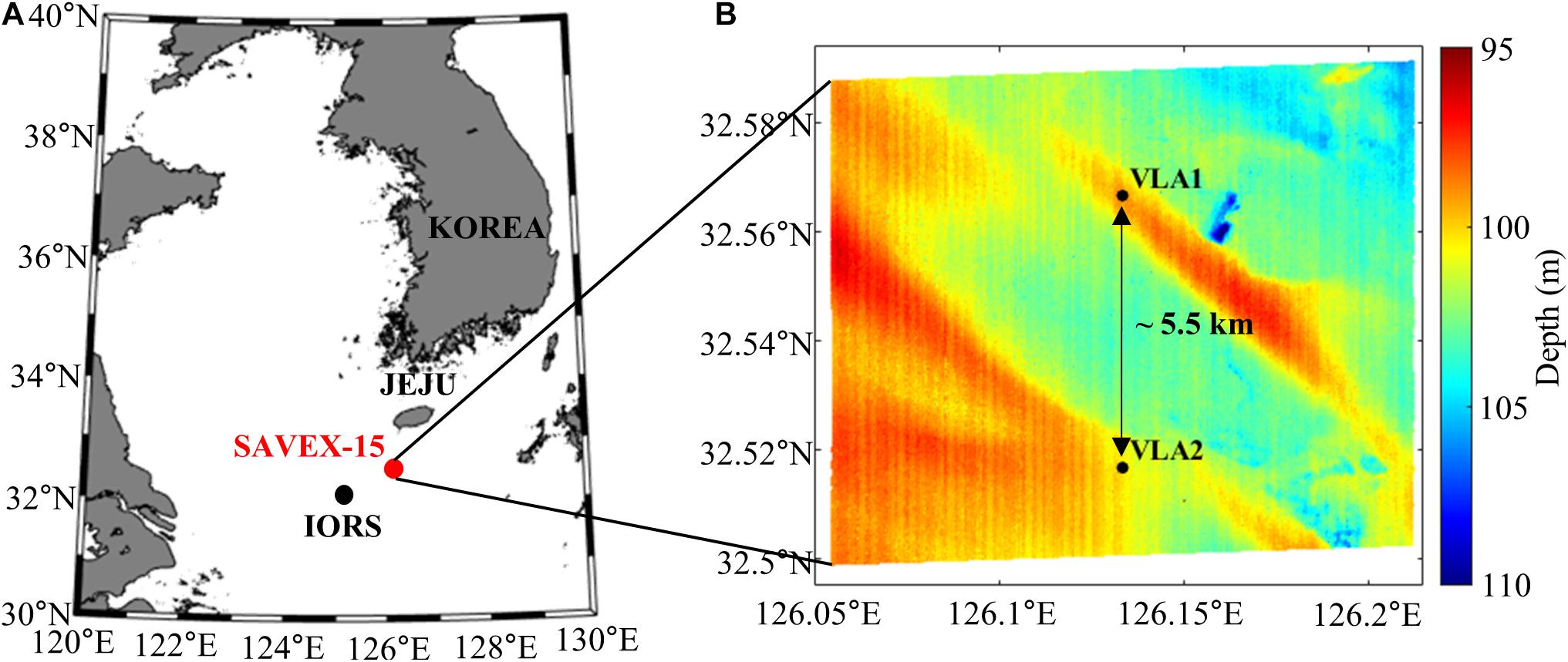
Figure 1. (A) Location of the experimental site (red circle) of SAVEX-15. The black dot denotes the IEODO ocean research station (IORS). (B) Topographic map of the experimental site including two vertical line arrays (VLAs) separated by 5.5 km: VLA1 and VLA2.

FIGURE 2

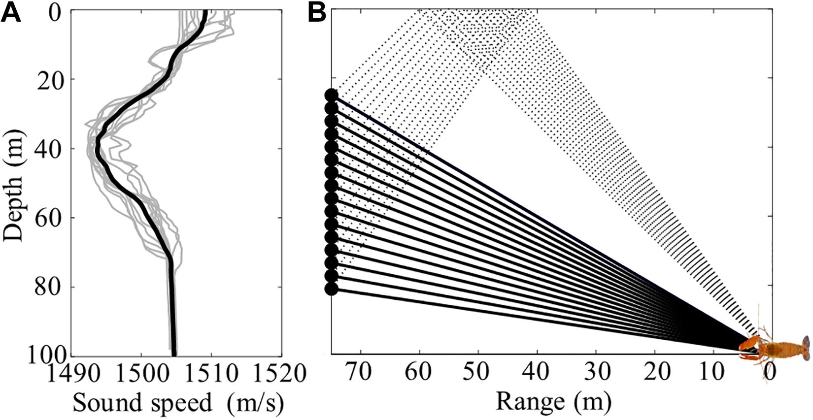
Figure 2. (A) Sound speed profiles measured by 12 conductivity-temperature-depth (CTD) casts and their mean sound speed profile (thick line) during the experiment. (B) Ray diagram showing two representative ray paths of snap sound generated by a snapping shrimp. The solid and dotted lines indicate direct and sea surface-reflected paths, respectively.

The acoustic data received by the VLAs were sampled at a 100-kHz sampling rate and saved at 1-min intervals. During the experiment, the soundscape was dominated by the snapping shrimp noise. Figure 3A shows ambient noise data for 1 min received by the bottom hydrophone of VLA1 at 81-m depth, in which numerous impulse-shaped signals are seen. The data were highpass-filtered at 2 kHz to remove the low frequency ambient noise. Figure 3B displays the arrival structure in time and array depth for a 100-ms time window marked in Figure 3A, on JD 141 (May 21) at 12:00:24 UTC. The first arrival, which is direct, was received at the hydrophones in order from the bottom to the top. The arrival angles were estimated to be between 75.6° (bottom) and 44.5° (top) in the downward direction with respect to the horizontal, assuming that the array tilt is negligible. The distance to the snapping shrimp on the seafloor was estimated to be about 75 m from the array by comparing the measured arrival angles and those predicted by a ray-based acoustic propagation model using the mean sound speed shown in Figure 2A. The second arrival, which was surface-reflected, was received at the hydrophones in order from the top to the bottom. The arrival angles were estimated to be between 22.4° (bottom) and 30.7° (top) in the upward direction, consistent with those predicted for the sea surface-reflected path for the same source location. The tilt angle of the VLA1 was estimated to be less than 3.2° around 16:00 on JD 145 (Yuan et al., 2018). Figure 3C shows a comparison of the measured arrival structure and predictions estimated from the eigenray tracing results shown in Figure 2B.

FIGURE 3

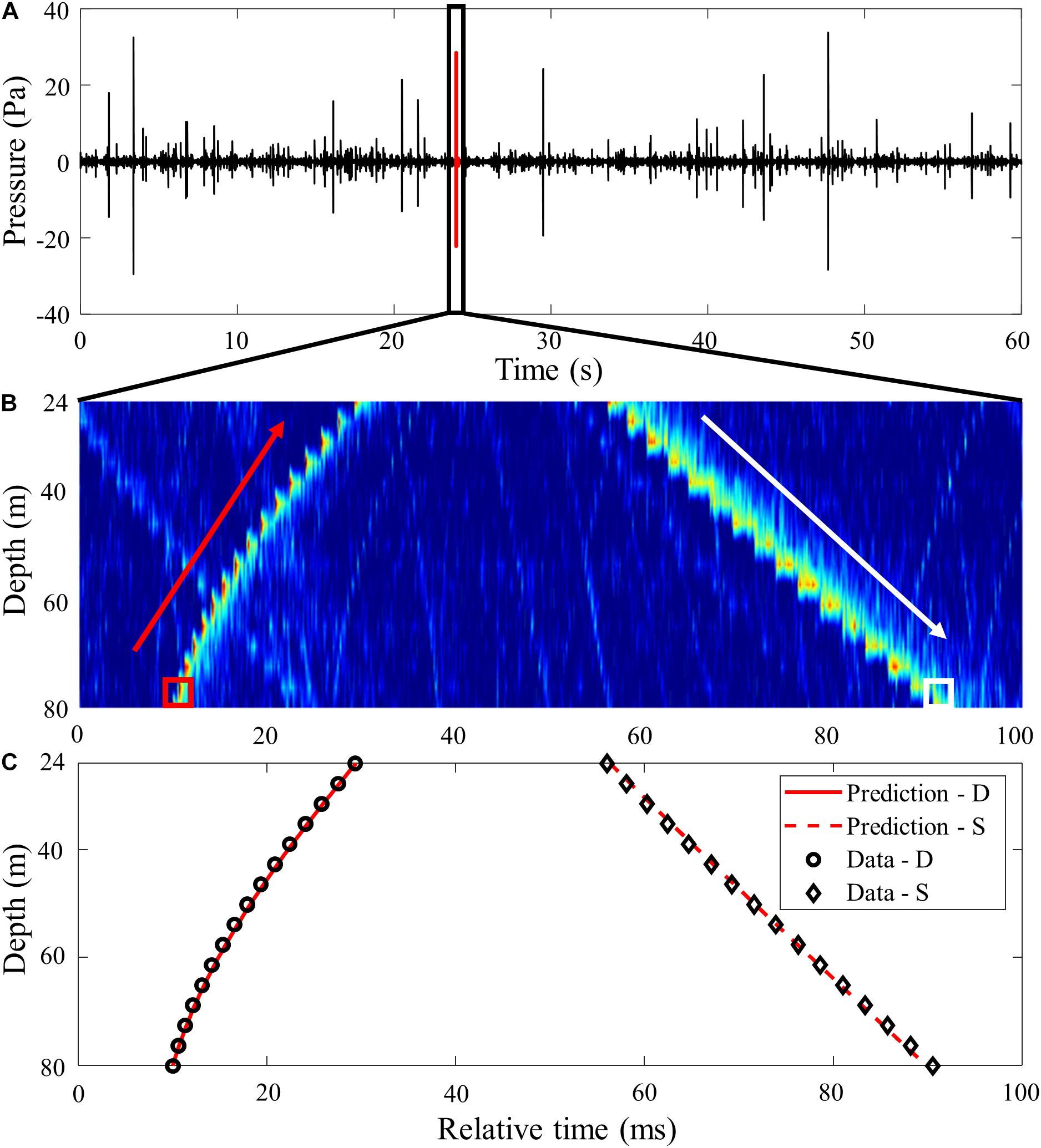
Figure 3. (A) Example of ambient noise data received for 1 min at the bottommost hydrophone (81 m) of VLA1 on JD 141 at 12:00 UTC, exhibiting many impulsive snapping shrimp noise. (B) Arrival structure of a single snapping shrimp noise in array depth and time over a 100-ms long time window, zoomed in on the black box in panel (A). The red arrow indicates that the snapping shrimp noise propagates spherically from the bottom to the sea surface, whereas the white arrow indicates a linear downward propagation of the sea surface-reflected snapping shrimp noise. (C) Model and data comparison for direct (D) and surface-reflected (S) arrival. The model assumes the source on the sea floor is at 75-m range from the array.

Note that there is a sharp distinction in acoustic properties between the direct arrival and the sea surface-reflected arrival. Figures 4A,B show the snapping shrimp noise for the direct (D) and the sea-surface (S) paths received by the bottom hydrophone of VLA1, respectively, corresponding to the signals marked by red and white boxes, respectively, in Figure 3B. The direct path is impulsive and strong, whereas the sea-surface bounced path undergoes a significant time spread caused by scattering from the rough sea surface with a smaller amplitude.

FIGURE 4

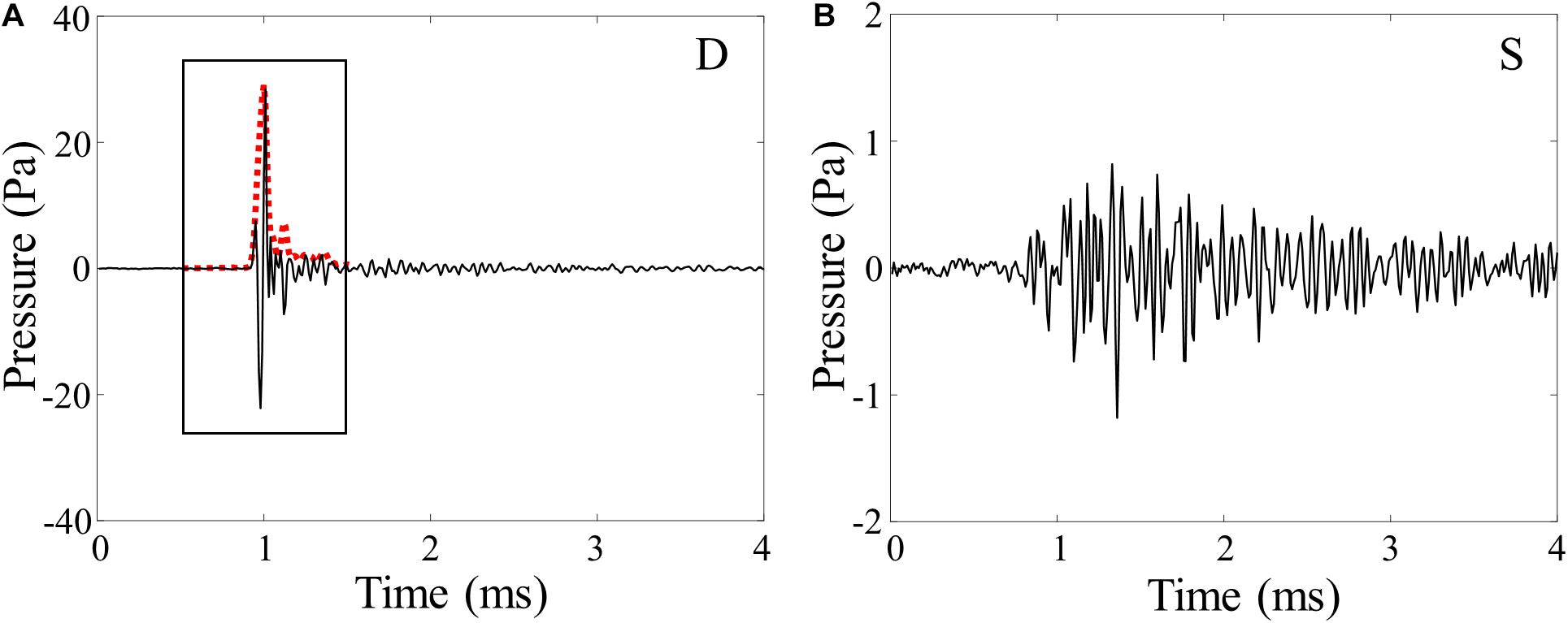
Figure 4. (A) Time series of the direct arrival (D) captured in the bottom red box in Figure 3B. The red dashed line indicates the 1-ms smoothed kernel envelope of the snapping shrimp noise. (B) The waveform of snapping shrimp noise reflected from the sea surface (S), captured in the bottom white box in Figure 3B. Note the different pressure scales.

Snap Detection Algorithm

To investigate the correlation between the snap rate and ocean environmental factors, it is necessary to accurately extract only the snapping shrimp waveforms from the received acoustic data. Recently, an envelope correlation combined with amplitude threshold detection algorithm (Bohnenstiehl et al., 2016; Lillis and Mooney, 2018) were used to extract the snapping events. In this paper, we applied the algorithm with some modifications to discard the waveform corresponding to the sea surface-reflected snapping noise. The 1-ms waveform displayed in the box of Figure 4A was Hilbert-transformed, and a three-point moving average was applied to extract a smoothed kernel envelope of the snapping shrimp waveform (red dashed line). The kernel envelope was then cross-correlated with a segmented signal envelope of the same length. After that, the time window in the signal envelope was advanced in steps of 0.5 ms along the time axis, and the cross-correlation process was applied repeatedly. Once the correlation coefficient value exceeded 0.8, the corresponding signal was selected. However, there were instances where one snapping event was initially counted twice in succession because the time window overlapped by 0.5 ms, which is half the length of the time window; we removed the double counts. Then, among the selected waveforms, only those whose peak amplitude exceeded four times the root-mean-square (rms) amplitude of the received signal were chosen as snapping shrimp events to reduce the probability of false detection due to ambient and system noise. Assuming a normal distribution, the amplitude of a signal that exceeds four times the rms value was in the upper 0.01% (Taylor, 1997).

Finally, it is important to avoid double-counting from the sea-surface bounce path for the same event. In this paper, we use kurtosis, which in statistics is a measure of the sharpness of the probability distribution (Abramowitz and Stegun, 1972), but here can be applied to measure the relative sharpness of the waveform shape. Unlike the direct path, the sea surface-reflected path usually undergoes a time spread (Figure 4B) due to scattering from the rough sea surface and microbubbles beneath the sea surface (Dahl, 1999; Choi and Dahl, 2006), thereby leading to a smaller kurtosis value. Figure 5A shows the kurtosis values for the direct (D, black circles) and sea surface (S, gray circles) paths from the analysis of 1,000 waveforms captured at the bottom hydrophone of VLA1 for 30 min from JD 142 00:00 UTC, which are well-separated (horizontal red line). The mean and standard deviation for the D and S are 20.2 ± 3.5 and 5.2 ± 1.6, respectively. Based on the histograms displayed in Figure 5B, the waveforms whose kurtosis values are >11.2 (denoted by a vertical line) were counted as the direct path from the snapping shrimp.

FIGURE 5

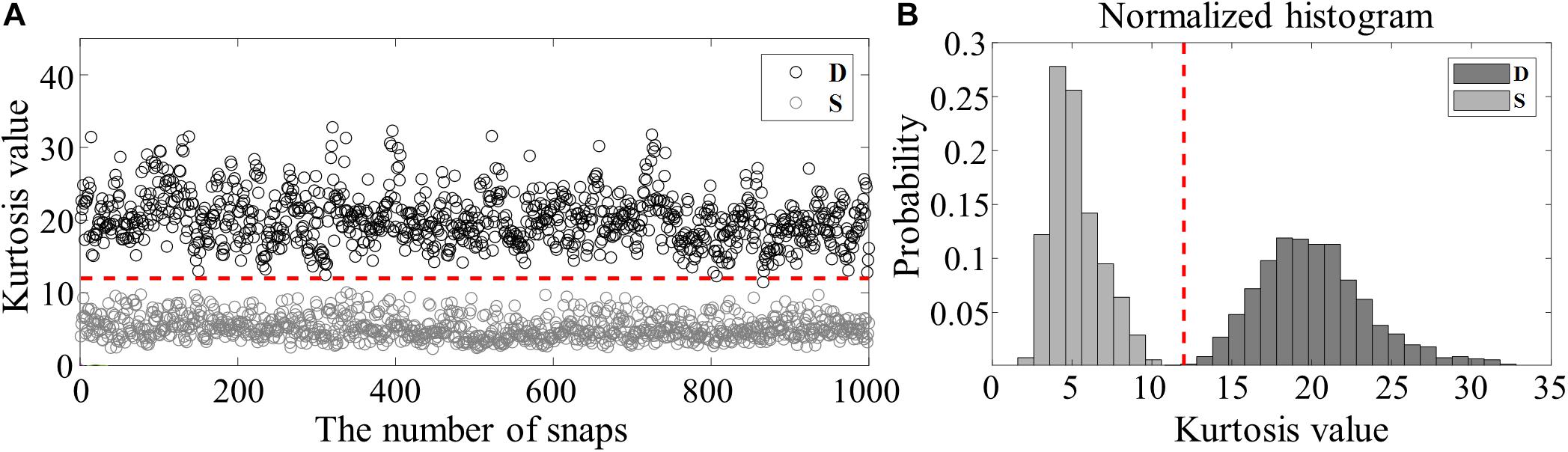
Figure 5. (A) Kurtosis values estimated from 1,000 waveforms for direct (D, black circles) and sea-surface reflected (S, gray circles) paths, which were collected by the bottom hydrophone of VLA1 for 30 min from JD 142 at 00:00 UTC. (B) Corresponding normalized histograms of kurtosis values for D (dark) and S (gray), respectively. The red vertical line denotes the kurtosis value of 11.2, which was selected as the criterion to filter out the S paths.

Results

Temporal Variation of Snap Rate

Figure 6A shows the temporal variation of the snap rate extracted from the bottommost hydrophones of VLA1 (solid) and VLA2 (dashed) over a 5-day period (JD 140–JD 145). The objective of SAVEX-15 was to collect acoustic and environmental data appropriate for studying the coupling of oceanography, acoustics, and underwater communications (Song et al., 2018), so acoustic transmissions were made intermittently in various frequency bands (0.5–32 kHz) throughout the experiment. Therefore, we excluded the data containing the broadcast signals for the analysis of snapping shrimp noise. First, we calculated the number of snaps per minute (gray and pink dots) during the 5 days, which were then smoothed out using a 90-point moving average filter (black solid and red dashed line in Figure 6A). Although the two arrays were ∼5.5 km apart, the temporal variations of the snap rate exhibit a nearly identical pattern between 200 and 1,200 snaps per minute. To examine the periodicity of the snap rate, we applied the Morse wavelet method (Lilly, 2016) to the VLA1 (solid line), which is shown in Figure 6B as a function of time and frequency. In contrast to the previous studies (Bohnenstiehl et al., 2016; Lillis and Mooney, 2018), this result reveals that there is a strong one-quarter-diurnal (four cycles per day) period with a relatively weak semi-diurnal (twice a day) period in the snap rate.

FIGURE 6

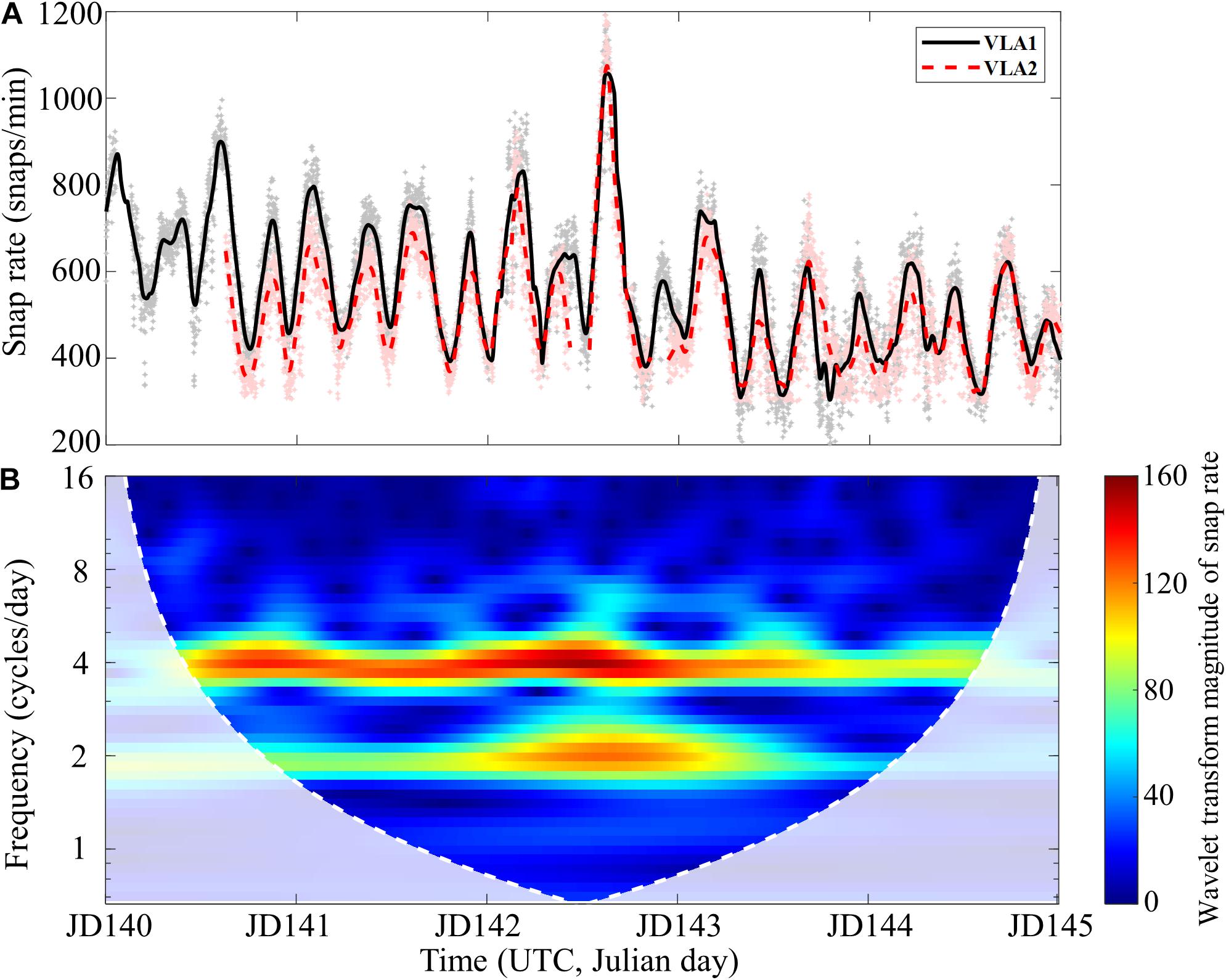
Figure 6. (A) Temporal variation of the snap rate extracted from the bottommost hydrophones of VLA1 (solid, gray dots) and VLA2 (dashed, pink dots) over a 5-day period (JD 140–JD 145). Each dot represents the snap rate calculated per minute, and a 90-point moving average produces the two smooth lines. Although the two arrays are separated by 5.5 km, the patterns are strikingly similar. (B) Magnitude scalogram of the snap rate at the VLA1 using the Morse wavelet method. The white dashed line marks the boundary of the cone of influence, and the shaded region below the line is affected by edge-effect artifacts. The scalogram highlights that the one-quarter-diurnal (four cycles per day) period is dominant in the snapping noise generated by the snapping shrimp inhabiting the SAVEX-15 area.

Correlation of Snap Rate and Environmental Factors

As mentioned earlier, the main difference between previous studies and our work is that the habitat of the snapping shrimp analyzed in this paper is an environment with minimal or no impact of the sunlight on the physical oceanic variabilities. The euphotic zone depth Z_eu is defined as the depth where the photosynthetic available radiation (PAR) value is 1% of the surface value (Kirk, 2010). It can be estimated indirectly by the empirical relationship between the chlorophyll-a (Chl-a) measured at the sea surface and Z_eu, which is given by (Morel et al., 2007)

$$log\left(Z_{eu}\right)=1.524-0.436X-0.0145X^2+0.0186X^3,(1)$$

where X = log(C_chl−a) and C_chl–a is the Chl-a concentration (mg/m³). The Chl-a concentration can be also indirectly measured by the Moderate Resolution Imaging Spectroradiometer (MODIS) on board satellite. Shang et al. (2011) compared Z_eu obtained from Eq. (1) using the Chl-a concentration estimated by the MODIS with the in situ Z_eu measured directly in the East China Sea, and showed that two values were highly correlated with an r-value of 0.95. The regional monthly mean sea surface Chl-a concentrations measured from the MODIS mounted on Aqua are available on the National Aeronautics and Space Administration (NASA) Ocean Color website¹. Using the regional monthly mean sea surface Chl-a concentrations corresponding to May 2015, the euphotic zone depth for the experimental site was estimated to be ∼30 m, meaning that sunlight hardly reaches the ocean depth of 100 m in the experimental site. Therefore it is worth noting that the habitat of the snapping shrimp in the current work is distinguished from the environments covered in previous studies (Johnson et al., 1947; Everest et al., 1948; Watanabe et al., 2002; Bohnenstiehl et al., 2016; Lillis and Mooney, 2018).

In an effort to identify the most significant factors affecting the snap rate of snapping shrimp living in the mesopelagic zone, we compare the temporal variability of the snap rate to the temporal variabilities of the following five environmental factors: the temperature profile in the water column, tidal level, current speed, wind speed, and significant wave height. Figure 7A shows the temporal variation of the temperature profile in the water column during the 8 days from JD 139 to JD 147. Overall, the temperature is lower in the middle layer, and increases toward the surface and the seafloor. Note that the boundaries of the cold water oscillate over time resulting from the non-linear internal waves observed in the area (Nam et al., 2018). We employed an empirical orthogonal function (EOF) analysis (Emery and Thomson, 2001) over only the first 4-day period from JD 139 to JD 143 (denoted by the dashed box) because the upper temperature data were not available in the second half.

FIGURE 7

Figure 7. (A) Temporal variation of the temperature profile in the water column measured at VLA1 during the experiment. (B) Amplitude of the first three empirical orthogonal function (EOF) modes for the temperature profiles measured during the first 4 days marked by the dashed box in panel (A). (C–E) Temporal variations of the first three EOF modes.

For the EOF analysis, the temperature profiles were demeaned, and then the eigenvalues and eigenvectors of the covariance matrix were calculated. The eigenvalues are arranged in a descending order to evaluate the percentage of the variance corresponding to each mode. The measured temperature profile, T(z,t) can be expressed as (Casagrande et al., 2011)

$$T(z,t)=\overline{T}\left(z\right)+{\sum }_{i=1}^M{\mathrm{\alpha }}_i(t)\cdot {\varphi }_i(z),(2)$$

where $\overline{T}\left(z\right)$ is the time-averaged temperature profile, α_i(t) is the amplitude of the ith orthogonal mode at time t, and ϕ_i(z) represents the ith EOF eigenmode. M is the total number of EOF mode considered in the EOF analysis. The first three EOF modes (EOF1, EOF2, and EOF3) are displayed along the depth in Figure 7B, and the temporal fluctuation of each mode amplitude is shown in Figures 7C–E, respectively. The first mode (EOF1) accounts for 46.5% of the total variation, while the first three modes account for 78.1%. Note that modes EOF1 (black) and EOF2 (blue) in Figure 7B concentrate in the upper and lower water column, respectively. As a result, the amplitude of EOF1 exhibits a strong correlation with the temporal variation of the upper thermocline with an r-value of 0.92 (see the upper black line in Figure 7A, which denotes the 13.5°C isotherm). On the other hand, EOF2 in Figure 7D is correlated with the temporal variation of the lower thermocline represented by the 13.5°C isotherm denoted by the lower blue line in Figure 7A with an r-value of 0.72. The EOF analysis indicates that the first three modes take into account most of the temperature variation in the water column, but the water temperature near the seafloor inhabited by snapping shrimp remained unchanged at about 14°C. The CTD casts made during the measurement period also confirmed that the sound speed dependent on the water temperature was almost constant near the seafloor (see Figure 2A). In summary, we did not find any evidence to support the correlation between the snap rate and water temperature as reported in the literature (Knowlton and Moulton, 1963; Watanabe et al., 2002; Jung et al., 2012; Bohnenstiehl et al., 2016).

The tidal variation can be deduced from the in situ tidal measurement at the nearby IEODO ocean research station (IORS) ∼100 km southwest of the SAVEX-15 area (Figure 1A) because the tidal phase difference between the two regions can be computed from the mean high-water intervals (MHWI) provided by the Korea Hydrographic and Oceanographic Agency (KHOA) website.² For Korean waters, the MHWI is defined as the mean time lag between the transit of the moon over the meridian 135° east and the following high water at a given location. The tidal phase of our experimental site was estimated to be 4 min faster than that of IORS. In Figure 8, the extrapolated tide (blue line) from JD 140 to JD 145 indicates a strong semi-diurnal period in the region, in contrast with the one-quarter-diurnal cycle of the snap rate (Figure 6A). However, it appears that the snap rate tends to peak at both high and low tides with some time lag.

FIGURE 8

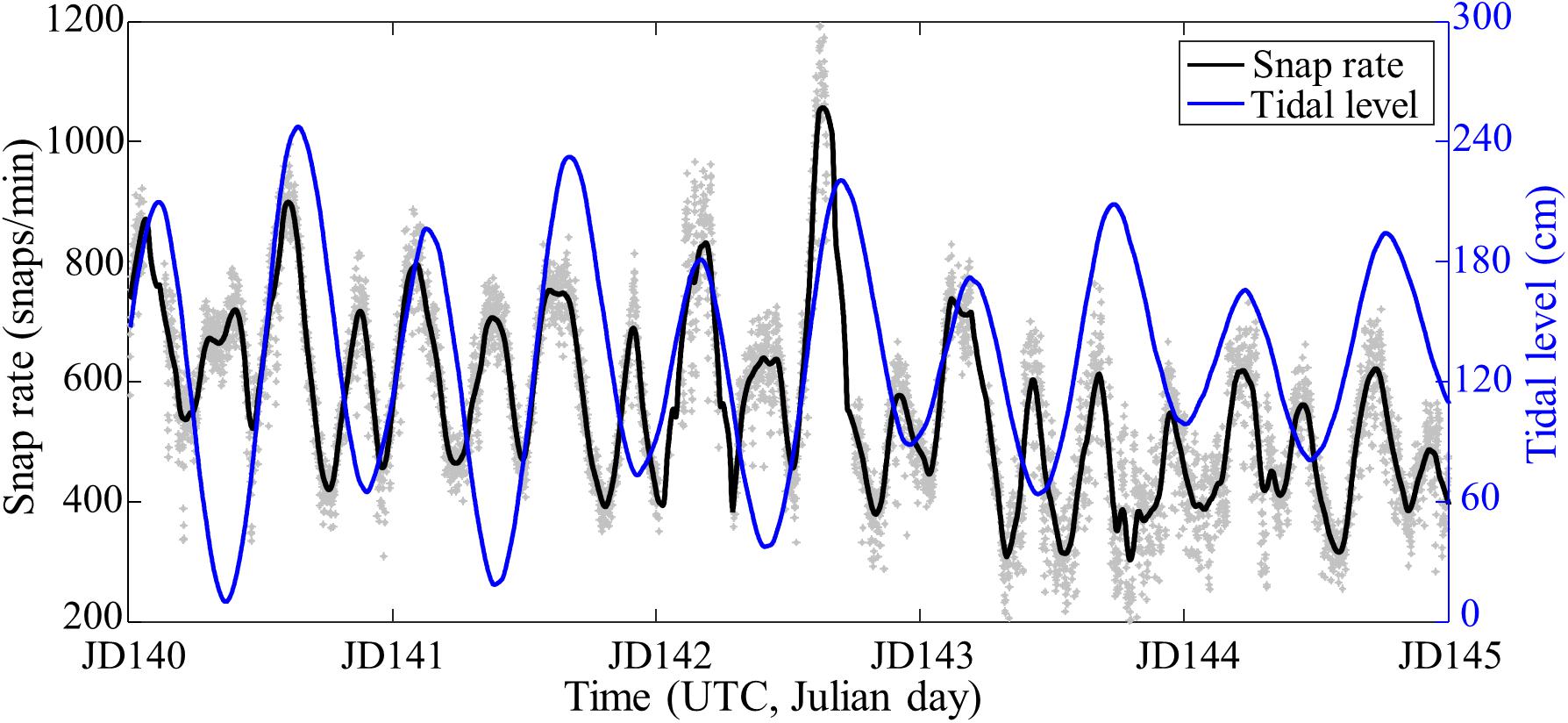
Figure 8. Reproduction of Figure 6A at VLA1 (gray dots and black line). The extrapolated tidal level (blue line) is superimposed for comparison.

The snap rate is now compared to the current since the tide affects the current. During the experiment, we collected the current data intermittently using a 150-kHz acoustic Doppler current profiler (ADCP) installed on the R/V Onnuri, while stationed about 5 km southwest of the VLA1. Figures 9A,B show the zonal (U_i) and meridional (V_i) components of the current velocity measured at 8-m intervals between 17 and 65 m of water depth and their respective mean values (thick black circles). Overall, the water column moves in the same direction (i.e., barotropic) with a semi-diurnal cycle, indicating the dominance of the tidal current in the region (Turgut et al., 2013; Noh et al., 2014; Lozovatsky et al., 2015). The current speed estimated by $\sqrt{{\overline{U}}^2+{\overline{V}}^2}$, where the upper bar denotes an average over depth, is presented in Figure 9C (blue line) along with the tide (black line) estimated at VLA1 site throughout the experiment (JD 135–JD 145). The local maximum of the current speed occurs at both high and low tides (vertical dashed lines), consistent with the characteristic of progressive tidal wave in open ocean (Parker, 2007; Hicks, 2013). As a result, the current speed exhibited a quarter-diurnal period as observed in the snap rate (Figure 8).

FIGURE 9

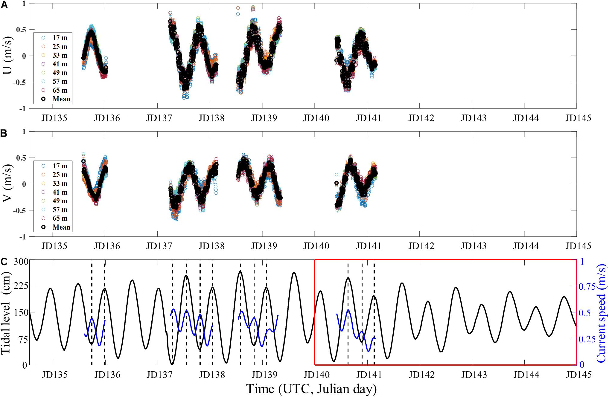
Figure 9. Time series of (A) zonal and (B) meridional components of the current velocity measured at various depths and their respective mean values (thick black circles). (C) The mean current speed (blue line) computed from panels (A,B) is superimposed on the tide (black line) at VLA1 site throughout the experiment (JD 135–JD 145). The vertical dashed lines denote the times of high and low tides. Our snap rate was estimated during the period in the red box (JD 140–JD 145).

To confirm the correlation between the snap rate and current speed, we focus on the short period (JD 140.4–JD 141.2) when both the current data and snap rate are available. The detrended current speed (blue) and snap rate (black) are shown in Figure 10A, indicating a strong correlation with a time lag. In fact, the cross-correlation has the maximum (r = 0.87) at 1 h and 15 min (1.25 h) in Figure 10B, meaning that the snap rate peaks 1.25 h prior to the local maximum current.

FIGURE 10

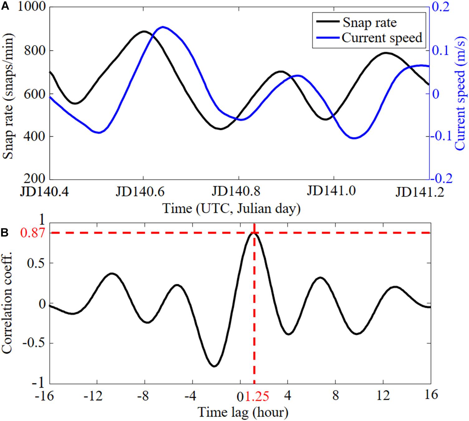
Figure 10. (A) Comparison between the snap rate (black) and current speed (blue) from JD 140.4 to JD 141.2 (see Figure 9C). (B) Cross-correlation between snap rate and current speed. The maximum correlation indicates that the snap rate peaks 1.25 h before the local maximum current.

Lastly, the snap rate was compared to the wind speed and the significant wave height at the time of measurements. The wind speed was measured by a vessel-mounted auto weather station (AWS), while the significant wave height was measured by a directional waverider buoy (DWR-G4, Datawell). These two environmental factors, however, did not show any pattern relevant to the snap rate.

Summary and Discussion

The sound generated by snapping shrimp is the dominant source of ambient noise in shallow coastal waters, especially at low to mid-latitudes. This sound has a strong peak energy and a wide frequency range, and greatly fluctuates in space and time. Although there have been several studies on which ocean environmental factors influence the snap rate, most studies were confined to the data observed at very shallow waters with a depth of a few tens of meters or less that sunlight reaches (euphotic zone). In contrast, we report the snapping shrimp sound observed at a depth of ∼100 m where sunlight does not reach. The temporal variation of the snap rate was investigated using the ambient noise data collected by two hydrophones at 81 m separated by 5.5 km during a 5-day period. Interestingly, the fluctuation of the snap rate at two sites was strikingly similar despite the distance. Second, the pattern exhibited a strong one-quarter-diurnal cycle, which, to our knowledge, has not previously been reported in the literature.

We compared the temporal variability of the snap rate to the temporal variabilities of the five environmental factors: the temperature profile in the water column, tidal level, current speed, wind speed, and significant wave height. It was found that the snap rate had a high correlation with the current speed in the experimental area where the barotropic tidal current is dominant. Interestingly, there was a time lag of about 1.25 h between the snap rate and current speed. It is beyond the scope of this work to investigate the cause of the time lag, including consideration of the biological characteristics of snapping shrimp. Lastly, because the snap rate change for only 5 consecutive days was unfortunately observed in this study, it was impossible to compare it with the long-term variability of ocean environmental factors such as seasonal or monthly variations performed in previous studies. Therefore, future work should involve long-term observations (monthly or seasonal) and collaboration with marine biologists to understand the acoustic behavior of snapping shrimp inhabiting the area where sunlight hardly reaches.

Data Availability Statement

The datasets presented in this article are not readily available because this experiment was performed with the supports of U.S. Office of Naval Research. Thus, the datasets are not uploaded to a publicly accessible repository. Requests to access the datasets should be directed to JC, choijw@hanyang.ac.kr.

Ethics Statement

Ethical review and approval was not required for the animal study because this study is not an ethically questionable study. This is a study on the sound produced by snapping shrimp.

Author Contributions

DL, JC, and HS: primary writing. DL, JC, SS, and HS: synthesis and overall coordination. HS: experiment design and data collection. DL and JC: acoustic data analysis. DL, JC, and SS: ocean environment data analysis. All authors discussed the results and contributed to writing through discussion, and reviewed the manuscript.

Funding

The SAVEX-15 was performed with the supports of U. S. Office of Naval Research and Korea Institute of Ocean Sciences and Technology. This work was also supported by the National Research Foundation of Korea (NRF) grant funded by the Korea Government (MSIT) (2020R1A2C2007772).

Conflict of Interest

The authors declare that the research was conducted in the absence of any commercial or financial relationships that could be construed as a potential conflict of interest.

Publisher’s Note

All claims expressed in this article are solely those of the authors and do not necessarily represent those of their affiliated organizations, or those of the publisher, the editors and the reviewers. Any product that may be evaluated in this article, or claim that may be made by its manufacturer, is not guaranteed or endorsed by the publisher.

Acknowledgments

We would like to thank SungHyun Nam and Seung-Woo Lee in Seoul National University, South Korea and Sung Hyup You in Korea Meteorological Administration for providing valuable comments on the characteristics of physical oceanography of the SAVEX-15 area.

Footnotes

1. ^ http://oceancolor.gsfc.nasa.gov/
2. ^ https://www.khoa.go.kr/

References

Abramowitz, M., and Stegun, I. A. (1972). Handbook of Mathematical Functions With Formulas, Graphs, and Mathematical Tables. Washington, DC: U.S. Department of Commerce.

Google Scholar

Au, W. W. L., and Banks, K. (1998). The acoustics of the snapping shrimp Synalpheus parneomeris in Kaneohe Bay. J. Acoust. Soc. Am. 103, 41–47. doi: 10.1121/1.423234

CrossRef Full Text | Google Scholar

Bohnenstiehl, D. R., Lillis, A., and Eggleston, D. B. (2016). The curious acoustic behavior of estuarine snapping shrimp: temporal patterns of snapping shrimp sound in sub-tidal oyster reef habitat. PLoS One 11:e0143691. doi: 10.1371/journal.pone.0143691

PubMed Abstract | CrossRef Full Text | Google Scholar

Casagrande, G., Stephan, Y., Varnas, A. C. W., and Folegot, T. (2011). A novel empirical orthogonal function (EOF)-based methodology to study the internal wave effects on acoustic propagation. IEEE J. Ocean. Eng. 36, 745–759. doi: 10.1109/JOE.2011.2161158

CrossRef Full Text | Google Scholar

Cato, D., and Bell, M. (1992). Ultrasonic Ambient Noise in Australian Shallow Waters at Frequencies Up to 200 kHz. Technical Report. Urbana: DSTO Materials Research Laboratory.

Google Scholar

Chitre, M. A., Potter, J. R., and Ong, S.-H. (2006). Optimal and near-optimal signal detection in snapping shrimp dominated ambient noise. IEEE J. Ocean. Eng. 31, 497–503. doi: 10.1109/JOE.2006.875272

CrossRef Full Text | Google Scholar

Choi, J. W., and Dahl, P. H. (2006). Measurement and simulation of the channel intensity impulse response for a site in the East China Sea. J. Acoust. Soc. Am. 119, 2677–2685. doi: 10.1121/1.2189449

CrossRef Full Text | Google Scholar

Dahl, P. H. (1999). On bistatic sea surface scattering: field measurements and modeling. J. Acoust. Soc. Am. 105, 2155–2169. doi: 10.1121/1.426820

CrossRef Full Text | Google Scholar

Emery, W. J., and Thomson, R. E. (2001). “Chapter 4 - The spatial analyses of data fields,” in Data Analysis Methods in Physical Oceanography, eds W. J. Emery and R. E. Thomson (Amsterdam: Elsevier Science), 305–370. doi: 10.1016/b978-044450756-3/50005-8

CrossRef Full Text | Google Scholar

Everest, F. A., Young, R. W., and Johnson, M. W. (1948). Acoustical characteristics of noise produced by snapping shrimp. J. Acoust. Soc. Am. 20, 137–142. doi: 10.1121/1.1906355

CrossRef Full Text | Google Scholar

Hicks, S. D. (2013). Understanding Tides. Silver Spring, MD: National Oceanic and Atmospheric Administration.

Google Scholar

Johnson, M. W., Everest, F. A., and Young, R. W. (1947). The role of snapping shrimp (Crangon and Synalpheus) in the production of underwater noise in the sea. Biol. Bull. 93, 122–138. doi: 10.2307/1538284

CrossRef Full Text | Google Scholar

Jung, S.-K., Choi, B. K., Kim, B.-C., Kim, B.-N., Kim, S. H., Park, Y., et al. (2012). Seawater temperature and wind speed dependences and diurnal variation of ambient noise at the snapping shrimp colony in shallow water of Southern Sea of Korea. Jpn. J. Appl. Phys. 51:07GG09. doi: 10.1143/jjap.51.07gg09

PubMed Abstract | CrossRef Full Text | Google Scholar

Kim, B.-N., Hahn, J., Choi, B. K., and Kim, B.-C. (2010). Snapping shrimp sound measured under laboratory conditions. Jpn. J. Appl. Phys. 49:07HG04. doi: 10.1143/jjap.49.07hg04

PubMed Abstract | CrossRef Full Text | Google Scholar

Kirk, J. T. O. (2010). Light and Photosynthesis in Aquatic Ecosystems, 3rd Edn, Vol. 4. Cambridge: Cambridge University Press, 1–651. doi: 10.1017/CBO9781139168212

CrossRef Full Text | Google Scholar

Knowlton, R. E., and Moulton, J. M. (1963). Sound production in the snapping shrimps Alpheus (Crangon) and Synalpheus. Biol. Bull. 125, 311–331. doi: 10.2307/1539406

CrossRef Full Text | Google Scholar

Lammers, M. O., Brainard, R. E., Au, W. W., Mooney, T. A., and Wong, K. B. (2008). An ecological acoustic recorder (EAR) for long-term monitoring of biological and anthropogenic sounds on coral reefs and other marine habitats. J. Acoust. Soc. Am. 123, 1720–1728. doi: 10.1121/1.2836780

CrossRef Full Text | Google Scholar

Legg, M. W., Duncan, A. J., Zaknich, A., and Greening, M. V. (2007). “Analysis of impulsive biological noise due to snapping shrimp as a point process in time,” in Proceedings of the OCEANS 2007 - Europe, Aberdeen, 1–6. doi: 10.1109/OCEANSE.2007.4302279

CrossRef Full Text | Google Scholar

Lillis, A., and Mooney, T. A. (2018). Snapping shrimp sound production patterns on Caribbean coral reefs: relationships with celestial cycles and environmental variables. Coral Reefs 37, 597–607. doi: 10.1007/s00338-018-1684-z

CrossRef Full Text | Google Scholar

Lilly, J. (2016). jLab: A Data Analysis Package for Matlab, v. 1.6. 2. Available online at: http://www.jmlilly.net/jmlsoft.html (accessed September 10, 2021).

Google Scholar

Lohse, D., Schmitz, B., and Versluis, M. (2001). Snapping shrimp make flashing bubbles. Nature 413, 477–478. doi: 10.1038/35097152

PubMed Abstract | CrossRef Full Text | Google Scholar

Lozovatsky, I., Jinadasa, P., Lee, J.-H., and Fernando, H. J. (2015). Internal waves in a summer pycnocline of the East China Sea. Ocean Dyn. 65, 1051–1061. doi: 10.1007/s10236-015-0858-2

CrossRef Full Text | Google Scholar

Morel, A., Huot, Y., Gentili, B., Werdell, P. J., Hooker, S. B., and Franz, B. A. (2007). Examining the consistency of products derived from various ocean color sensors in open ocean (Case 1) waters in the perspective of a multi-sensor approach. Remote Sens. Environ. 111, 69–88. doi: 10.1016/j.rse.2007.03.012

CrossRef Full Text | Google Scholar

Nam, S., Kim, D.-J., Lee, S.-W., Kim, B. G., Kang, K.-M., and Cho, Y.-K. (2018). Nonlinear internal wave spirals in the northern East China Sea. Sci. Rep. 8:3473. doi: 10.1038/s41598-018-21461-3

PubMed Abstract | CrossRef Full Text | Google Scholar

Noh, S.-Y., Seung, Y. H., Lim, E.-P., and You, H.-Y. (2014). Characteristics of semi-diurnal and diurnal currents at a KOGA station over the East China Sea shelf. Ocean Polar Res. 36, 59–69. doi: 10.4217/OPR.2014.36.1.059

CrossRef Full Text | Google Scholar

Nolan, B., and Salmon, M. (1970). The behavior and ecology of snapping shrimp (Crustacea: Alpheus heterochelis and Alpheus normanni). Forma Funct. 2, 289–335.

Google Scholar

Parker, B. B. (2007). Tidal Analysis and Prediction. Silver Spring, MD: NOAA.

Google Scholar

Shang, S. L., Lee, Z. P., and Wei, G. M. (2011). Characterization of MODIS-derived euphotic zone depth: results for the China Sea. Remote Sens. Environ. 115, 180–186. doi: 10.1016/j.rse.2010.08.016

CrossRef Full Text | Google Scholar

Song, H., Cho, C., Hodgkiss, W., Nam, S., Kim, S.-M., and Kim, B.-N. (2018). Underwater sound channel in the northeastern East China Sea. Ocean Eng. 147, 370–374. doi: 10.1016/j.oceaneng.2017.10.045

CrossRef Full Text | Google Scholar

Taylor, J. R. (1997). An Introduction to Error Analysis. Sausalito, CA: University Science Books.

Google Scholar

Turgut, A., Mignerey, P. C., Goldstein, D. J., and Schindall, J. A. (2013). Acoustic observations of internal tides and tidal currents in shallow water. J. Acoust. Soc. Am. 133, 1981–1986. doi: 10.1121/1.4792141

CrossRef Full Text | Google Scholar

Versluis, M., Schmitz, B., Von der Heydt, A., and Lohse, D. (2000). How snapping shrimp snap: through cavitating bubbles. Science 289, 2114–2117.

Google Scholar

Watanabe, M., Sekine, M., Hamada, E., Ukita, M., and Imai, T. (2002). Monitoring of shallow sea environment by using snapping shrimps. Water Sci. Technol. 46, 419–424. doi: 10.2166/wst.2002.0772

CrossRef Full Text | Google Scholar

Yuan, Z. Q., Richards, E. L., Song, H. C., Hodgkiss, W. S., and Yan, S. F. (2018). Calibration of vertical array tilt using snapping shrimp sound. J. Acoust. Soc. Am. 144, 1203–1210. doi: 10.1121/1.5054089

CrossRef Full Text | Google Scholar