 Zunlei Liu1,2
 Yan Jin1,2Liping Yan1,2Yi Zhang1,2Hui Zhang1,2Chuyi Shen3
 Linlin Yang1,2*Jiahua Cheng1,2*
- 1East China Sea Fisheries Research Institute, Chinese Academy of Fishery Sciences, Shanghai, China
- 2Key Laboratory of East China Sea Fishery Resources Exploitation and Utilization, Ministry of Agriculture and Rural Affairs, Shanghai, China
- 3College of Economics and Management, Shanghai Ocean University, Shanghai, China
Identifying the spatio-temporal distribution hotspots of fishes and allocating priority conservation areas could facilitate the spatial planning and efficient management. As a flagship commercial fishery species, Largehead hairtail (Trichiurus japonicus) has been over-exploited since the early 2000s. Therefore, the spatio-temporal management of largehead hairtail nursery grounds could effective help its recovery. This study aims to predict juvenile largehead hairtail distribution patterns and identify priority conservation areas for nursery grounds. A two-stage hierarchical Bayesian spatio-temporal model was applied on independent scientific survey data (Catch per unit effort, CPUE) and geographic/physical variables (Depth, Distance to the coast, Sea bottom temperature, Dissolved oxygen concentration and Net primary production) to analyze the probability of occurrence and abundance distribution of juvenile largehead hairtail. We assessed the importance of each variable for explaining the occurrence and abundance. Using persistence index, we measured the robustness of hotspots and identified persistent hotspots for priority conservation areas. Selected models showed good predictive capacity on occurrence probability (AUC = 0.81) and abundance distribution (r = 0.89) of juvenile largehead hairtail. Dissolved oxygen, net primary production, and sea bottom temperature significantly affected the probability of occurrence, while distance to the coast also affected the abundance distribution. Three stable nursery grounds were identified in Zhejiang inshore waters, the largest one was located on the east margin of the East China Sea hairtail national aquatic germplasm resources conservation zones (TCZ), suggesting that the core area of nursery grounds occurs outside the protected areas. Therefore, recognition of these sites and their associated geographic/oceanic attributes provides clear targets for optimizing largehead hairtail conservation efforts in the East China Sea. We suggested that the eastern and southern areas of TCZ should be included in conservation planning for an effective management within a network of marine protected areas.
Introduction
Recruitment is a fundamental process in population dynamics, which is highly variable in time, space and vulnerable to fishing gear (Gaillard et al., 2008). Understanding the spatial pattern of juvenile distribution is of great interest to fishery science and marine ecology, since juvenile is a critical stage of fish stocks. Therefore, reducing the fishing effort with non-selective gears in recruitment areas will help avoid recruitment overfishing (Caddy, 2000; Paradinas et al., 2015). Considering the vulnerability of recruitment and their role in population dynamics and stock size fluctuation, the protection of important habitats is critical for the conservation of marine fish and even the conservation of biodiversity (Hunt et al., 2020). A recommended management tool is establishing a network of Fisheries Restricted Areas (FRA) in regions where the target species is known to aggregate during critical stages of their life cycle (Caddy, 2009, 2000; Colloca et al., 2015; Paradinas et al., 2015; Petza et al., 2019). However, ensuring the effectiveness of such protected areas requires a comprehensive understanding of species distribution and habitat relationships. This ecological knowledge is becoming increasingly important for the sustainable exploitation of commercially important marine populations (Colloca et al., 2015; Paradinas et al., 2015).
Linking the environmental processes and ecological interactions to recruitment success may help explain the dynamics of fish populations and their productivity (Zimmermann et al., 2019). Biogeographers studied the environmental drivers of recruitment distribution and variation at the regional and other extents and identified basin scale oceanographic processes as the key drivers (Castillo-Jordán et al., 2016; Koenigstein et al., 2016; Zimmermann et al., 2019). As powerful physical forces in the seas, oceanic currents have a major influence on the distribution of water masses, nutrients and the productivity of ecosystems, thus influencing the drift, dispersal, and settlement of fish at early life stages (White et al., 2019; Bashevkin et al., 2020). The thermal environments that organisms experience strongly affect their survival rates, distribution, and abundance (Kingsolver, 2009; Isaak et al., 2015). Therefore, temperature defines the habitat of a species’ realized thermal niche (Armstrong et al., 2021). Dissolved oxygen in the aquatic habitat is an important requirement for fish growth and survival, because the energetic demands of organisms increase with temperature and activity, and must be met by an adequate supply of oxygen (Smith and Delorme, 2010; Deutsch et al., 2020). In the California Current large marine, Keller et al. (2015) indicated that catch and species richness exhibited positive relationships with near-bottom oxygen concentration. However, fish and organisms have a different tolerance for low dissolved oxygen concentrations, for instance, pelagic fish require higher levels of dissolved oxygen, while benthic organisms such as crabs and shrimp are more tolerant to the lower oxygen concentration (Brennan et al., 2016). Environmental predictors have been used to accurately predict the distribution of species in several studies (Bateman et al., 2012; Albuquerque and Beier, 2015a,b; Young and Carr, 2015). Such analyses concluded that abiotic variables could be used to predict the location of irreplaceable areas for conservation efforts (Lomolino et al., 2010). At large marine ecosystem scales, average trends in recruitment capacity in each ecosystem were found to be significantly related to environmental variables (Britten et al., 2016). Therefore, a better understanding of the environmental preference, the temporal and spatial scales at which species move could provide information on habitat use for the effective management. The East China Sea (ECS) is situated in the western Pacific Ocean. It is a semi-enclosed marginal sea spanning an area of 744,000 km2. More than 50% of the harvested stocks are overexploited due to the unselective exploitation pattern (Teh et al., 2019) and opportunistic fishery behavior. The minimum mesh size of trawl fisheries had been implemented since 2004. Due to poor enforcement and reduced trawl selectivity, 43.59% of the catch in bottom trawl fisheries are low-valued feed-grade fish that dominated by juveniles of food fish (Zhang et al., 2020). Such an exploitation pattern hinders the achievement of Maximum Sustainable Yield (MSY) for fisheries, as required by the new fisheries law and total allowable catch guide policy during China’s 13th Five-Year Plan. The current annual amount of feed-grade fish in China has been estimated to be over 4 mmt, corresponding to a percentage of 34.7% of the overall catch (Zhang et al., 2020). The protection of main commercial species nurseries is increasingly viewed as a major step toward achieving more sustainable exploitation patterns.
Largehead hairtail (Trichiurus japonicus) is a flagship species in China. The annual catch in China was over 1.4 mmt in 2006 (see Chinese Fishery Statistical Yearbook, 2016), but declined to 0.92 mmt in 2019 (see Chinese Fishery Statistical Yearbook, 2019). Due to the wide distribution of spawning grounds and high fecundity, largehead hairtail catch remained high for a long time despite persistently high-intensity fishing pressure. Although largehead hairtail fisheries have shown a surprisingly high resilience to human exploitation than other fisheries, the most important commercial species is now fully exploited. Important negative impacts have also been detected, such as a high proportion of juvenile fish in the catch because of non-selective gears and fishing grounds overlap with the juvenile largehead hairtail distribution.
The Chinese government has taken a series of practical measures to address these problems. In 2010, the State Council issued and implemented the strategy and action plan for biodiversity conservation in China (2011–2030), which provided guidance for the priority areas of inland, water, ocean, and coastal biodiversity conservation. By 2019, China had established 271 protected areas that include oceans (Zhou et al., 2021). They cover 12.4 million hectares of the ocean but represent only 4.1% of China’s maritime area (Zhou et al., 2021). Because of small conservation areas, the ability to protect migratory fishes is likely hindered by their fragmentation. China holds an annual fishing moratorium lasting nearly 4 months in the Yellow Sea, the ECS, and the South China Sea and established ECS largehead hairtail national aquatic germplasm resources conservation zones (TCZ) to protect spawning and juvenile largehead hairtail stock. However, the current TCZ cannot keep up with the demand for effective resource protection. How to accurately identify and determine the priority reserve is a prerequisite for conservation activities. Accurate identification and determination of priority reserves can guide the rational allocation of resources and maximize the protection benefits (Wu et al., 2016).
Species distribution models (SDMs) have been widely used across terrestrial, freshwater, and marine realms to identify species-environment relationships and to identify priority areas, ‘hotspots’ of vulnerable species (Ovando et al., 2019; Pennino et al., 2019a; Lyons et al., 2020; Epele et al., 2021) or essential fish habitat (Colloca et al., 2015; Laman et al., 2018). A variety of methodological approaches have been developed over the last decades to generate SDMs, such as Neural Networks (Özesmi and Özesmi, 1999), Boosted Regression Trees (Elith et al., 2008; Wege et al., 2021), Maximum Entropy (Phillips et al., 2006), Generalized Linear Regression Model (Guisan et al., 2002), and Additive Regression Models (Swartzman et al., 1992; Austin, 2007). However, the statistical challenges using SDMs have increased as datasets have become more complex over time (Orúe et al., 2020; Lloret-Lloret et al., 2021). Recently, Bayesian hierarchical spatiotemporal models with the Integrated Nested Laplace Approximation (INLA) methodology has acquired an important role, since it is ideally suited for fitting complex spatiotemporal covariance structures (Rue et al., 2009; Silva et al., 2017). INLA provides accurate approximations to the posterior marginal distributions of latent Gaussian Markov Random Field (GMRF) models with considerably less computational effort (Rue and Held, 2005). INLA handles models with the additional advantage of integrating common modeling approaches and uncertainty analyses into a more general hierarchical framework. Because of these advantages, Bayesian methods are increasingly used in fisheries studies in recent years (Pennino et al., 2014, 2019a,2019b; Nikolioudakis et al., 2019; Cavieres et al., 2021; Hintzen et al., 2021).
This study aims to provide seminal information on the key marine areas of the largehead hairtail in ECS to support conservation efforts by elucidating the spatial relationship between largehead hairtail distribution and oceanography. To accomplish this, (i) species distribution models of the INLA-SPDE approach was developed using Generalized Additive Models (GAM) to define oceanographic features of key largehead hairtail habitats in the ECS and identify contributions of each predictor. (ii) abundance indices from model output to explore the spatial and temporal patterns of juvenile largehead hairtail abundance in the ECS. (iii) we discussed the results within the current conservation and draw attention to the main threats for the studied species. We argued that an improved understanding of the spatial distribution of largehead hairtail could help to determine and manage MPAs by taking into account sensitive habitats.
Materials and Methods
Study Area
East China Sea is a marginal sea of the northwest Pacific. It connects with the South China Sea and the Yellow Sea, with an average depth of only 370 m (Liu, 2013). The study area included the ECS continental shelf (20–150 m in depth) and southern waters of the Yellow Sea (20–80 m in depth). This area covers approximately 370,000 km2. ECS is a highly productive area in China due to the presence of the Yangtze River and locally oceanographic circulation that brings nutrients to the upper slope and shelf areas.
Oceanographic characteristics of the ECS include two major current systems: the coastal current and the Kuroshio warm current. The Kuroshio warm current is a strong western boundary current in the North Pacific Ocean, which plays an important role in transporting heat, nutrients, and pelagic migratory species from the subtropical zone to the subarctic zone (Uda, 1972; Ma et al., 2021). The coastal current has characteristics of low salinity and high nutrient content. The Subei coastal current flows to the southeast and keeps stable. The surface current of the ECS coastal current varies from winter to summer. In autumn and winter, it flows southward along the shore and northward in summer. April to May and September are the transition periods. The influx and strength of each current vary both seasonally and inter-annually due to the basin-scale climatic phenomenon. These currents and water masses provide the ECS with high primary productivity, making it a vital spawning and nursery grounds for commercially valuable fishes (Zhao, 1987; Teh et al., 2019).
In the study area, permanent spatial closures for trawl vessels have been in existence since 1955, and fishing activities are allowed only for the artisanal fleet. In 1995, the summer fishing moratorium system came into effect outside the forbidden fishing line of motor trawling. In particular, the seasonal closures for juvenile largehead hairtail are located at the inshore of middle-north ECS, in which trawling is forbidden from April to September.
Survey Data
The biological data used in this study were collected by a scientific demersal trawling surveys conducted from 2014 to 2017 within the China National Project. The demersal trawling surveys were carried out during spring (April 25 to May 28), summer (July 16 to September 2), autumn (October 18 to November 12), and winter (December 30 to February 10). The survey provides a spatio-temporal dataset of fishery-independent indices related to demersal species abundance and spatial distribution (Supplementary Figure 1). The survey design follows a systematic sampling design with sampling stations evenly distributed in the survey area at a 30’ interval between each pair (Liu et al., 2009a). However, due to the influence of weather conditions or topography roughness, the number of survey stations varied slightly from year to year, and the trawling time and sampling latitude and longitude were not completely consistent with expectations. Roughly 372–538 survey stations were actually completed every year. A standard bottom trawling gear (4 m × 100 mesh, cod-end mesh size 20 mm) was used for 60 min based on the standard sampling protocol for bottom trawling (Liu et al., 2009a). All marine organisms were classified into species, and the abundance and biomass for each species were standardized to the number of individuals/h and kg/h (catch per unit effort, CPUE) as a measure of relative fish abundance. The largehead hairtail were randomly sampled from each presence site, with each largehead hairtail measured AL, body weight, sex, and gonadal maturity. Juveniles were considered individuals that had finished their larval phase but still had not reached first sexual maturity (Criscoli et al., 2017). However, the transition between larval and juvenile development remains ill defined, Colloca et al. (2015) assumed that the first separable modal component of the age group 0 as recruits, we operationally defined juveniles as within the smallest size at sexual maturity in anal length (AL 123 mm) followed Jin et al. (2020), the corresponding age is about 3–5 months according to early growth (Sun et al., 2020a). Sex identification for partial juveniles was difficult, so we pooled all the juveniles together regardless of gender for each site.
We created a Kernel Density Estimation (KDE) layer that provided an estimate of the probability to find juveniles presence points for each pixel (Figure 1), KDE recognized clusters or holes and gave intuitive perspective to examine significant concentrations of occurrence. KDE was calculated with the ‘kde2d’ function of the MASS package (Venables and Ripley, 2002) in the R platform on the extent of the ECS region (n and lims parameters defined to fit a raster layer of extent (118, 128, 23, 36) and number of grid points in each direction are set to 100, with a 0.1 degree and 0.03 degree of longitude/latitude grid). The occurrence distribution was variable over the ECS domain through this period, with most occurrence locations concentrated off the inshore of Central Zhejiang Province.
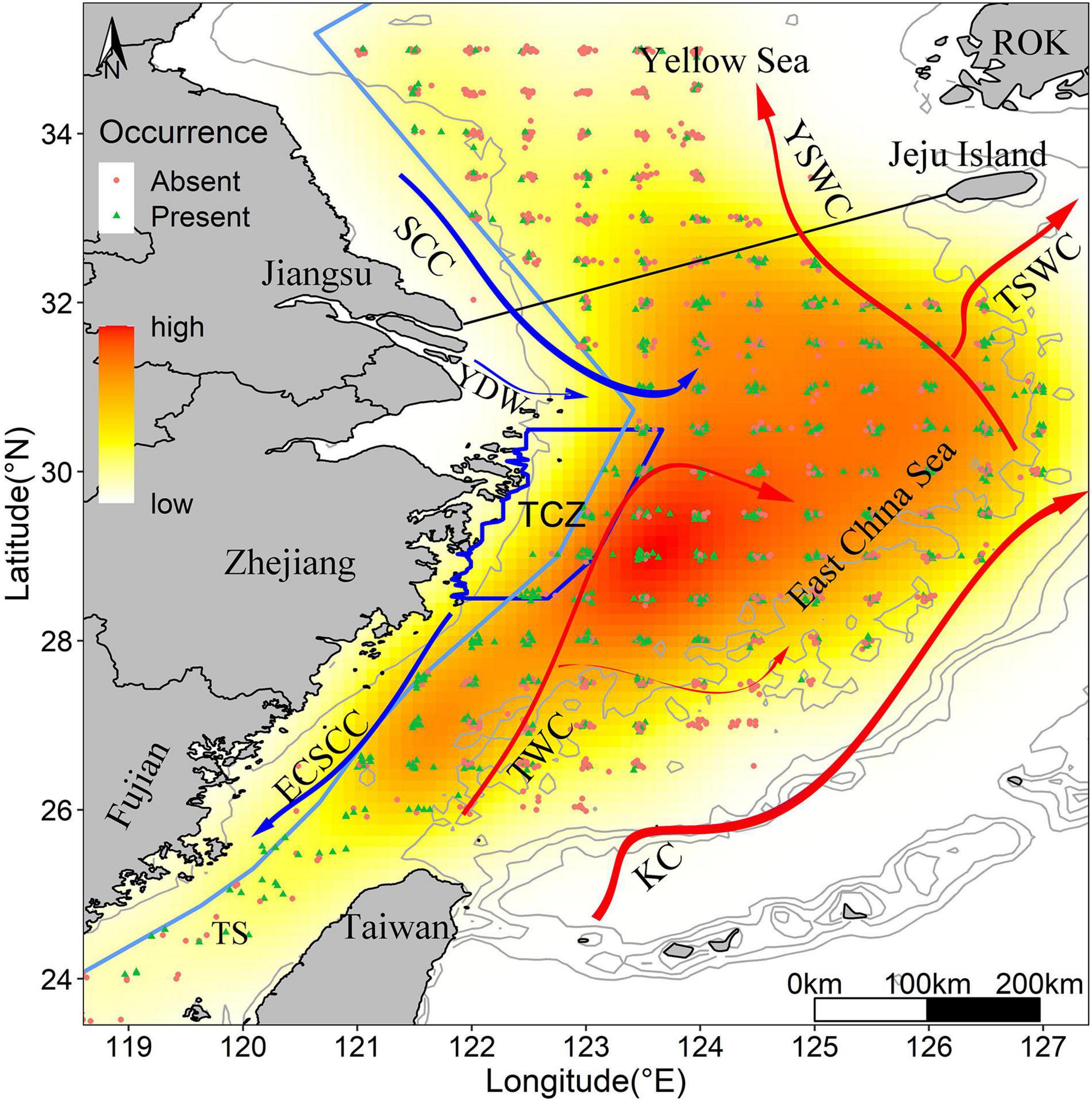
Figure 1. Kernel density map of survey samples in the ECS from 2014 to 2017. Yellow to red shading shows the intensification of occurrence probability. The blue dots and red dots refer to the presence points and absence points, respectively. Blue polygon indicates the largehead hairtail conservation zones. The light blue line along the continental coast represents trawl fishing forbidden line. Isobaths of 20, 100, 200, 500, and 1,000 m are indicated. Red and blue solid lines represent warm and cold currents, respectively (KC, Kuroshio Current; TSWC, Tsushima Warm Current; YSWC, Yellow Sea Warm Current; TWC, Taiwan Warm Current; ECSCC, East China Sea Coastal Current; SCC, Subei Coastal Current; YDW, Yangtze River diluted water). ROK represents Republic of Korea.
Environmental Data
Topographic variables and oceanographic variables were used as predictors of largehead hairtail occurrence and abundance. Due to a lack of detail observational data available in this region, topographic variables data were obtained from the Global Marine Environmental Datasets (GMED1) with a 0.083° × 0.083° spatial resolution. Oceanographic variables were extracted from the European Union Copernicus Marine Environmental Monitoring Service (CMEMS2) with a spatial resolution of 0.25° × 0.25° and a time resolution of daily. The CMEMS was used to act as our data for modeling because CMEMS assimilates a number of observation data sources, and previous findings indicated that the data assimilation technique can produce a reliable dataset (Edwards et al., 2015; Martin et al., 2015). Indeed, numerous studies employed the CMEMS to evaluate their observational data or produced ocean model in ECS and South China Sea (Lin et al., 2017; Lee et al., 2020; Sun et al., 2020b; Kok et al., 2021; Wu et al., 2021). Three topographic variables and six oceanographic variables were extracted for each position and date of the survey dataset, all variables were downscaled using a bilinear interpolation to match our fisheries data. The environmental factors included were as follows: bathymetry (Depth, m), distance to the coast (Disland, 100 km), slope, sea bottom temperature (SBT, °C), sea bottom salinity (SBS, psu), chlorophyll-a concentration (CHL, mg m–3), dissolved oxygen concentration (DO, mmol m–3), total phytoplankton (PHYC, mg m–3), and net primary production (NPPV, mg m–3). Terrain ruggedness index (TRI) provides a measure of the complexity of the seafloor and emphasizes small variations in the seabed terrain (Pennino et al., 2019a). It was derived from the continuous bathymetry using the raster package (Hijmans, 2016) in R (R Core Team, 2020).
In addition to the topographic and oceanographic variables, largehead hairtail conservation zone was considered as a covariate that may help to explain the necessity or accuracy of marine spatial planning. The TCZ is located in the middle area of the north-central ECS. The protection period of the core area is from April 16th to September 16th every year, during which trawling is prohibited. TCZ was considered a variable according to whether the survey station occurred in or out of TCZ.
Before running the models, the explanatory variables were standardized (difference from the mean divided by the corresponding standard deviation) to facilitate interpretation and compare relative weights between variables (Abada et al., 2020; Orúe et al., 2020). All environmental variables were tested for outliers, missing values, and correlation (Zuur et al., 2009a). Points on the far end along the horizontal axis (extremely large or extremely small values) were considered outliers by Cleveland dotplots. There were two relatively larger values for NPPV and one for TRI, PHYC, and CHL, respectively. These values were corrected by replacing them by a prediction value interpolated from the values of the four nearest cells. Missing values were not found in datasets. Correlation among variables was checked by performing Pearson correlation coefficient and Spearman correlation coefficient with the ‘Hmisc’ package (Harrell, 2021) and visualized the results using ‘corrplot’ package (Wei and Simko, 2017) in R. Pairs of variables with high correlation values (| r| > 0.7) were identified, and only one was included in the modeling process according to the ecological interpretation or the extent of collinearity. In addition, collinearity was assessed using the variance inflation factor analysis (VIF), the ‘corvif’ function with the code HighstatLibV10.R, and a cutoff value of 3 (Zuur and Ieno, 2017). Based on these preliminary analyses, High correlations were found between CHL and PHYC (r = 0.96), CHL and NPPV (r = 0.80), PHYC and NPPV (0.87), and between Slope and TRI (r = 0.87) (Supplementary Figure 2). Spearman correlation gave similar results but higher correlation was detected between Depth and SBS (r = 0.74), Depth and NPPV (r = –0.73) (Supplementary Figure 2). Variables with VIF > 3 included PHYC, CHL, NPPV, Slope, TRI and Depth (Supplementary Table 1). Considering that numerous studies reported strong relationships between NPPV and catch within regions or subsets of systems (Iverson, 1990; Chassot et al., 2007), and many of ecosystem models relied on NPPV as a forcing variable (Heneghan et al., 2021). Therefore, CHL and PHYC were removed from variables and NPPV was preserved for further analysis. Both of Slope and TRI provides an interpretation of the seabed features, we dropped the slope variable as it showed the stronger VIF index value. We retained Depth variable that was likely to be more ecologically relevant in explaining the distribution of largehead hairtail in the ECS (Du et al., 2020). We then repeated VIF process and found all VIF values were smaller than 3 (Zuur et al., 2009b) (Supplementary Table 1). As a result, Slope, CHL, and PHYC were eliminated for the posterior modeling due to the high correlation and collinearity. Finally, seven environmental variables were selected as explanatory predictors for the statistical models: Depth, TRI, Disland, SBT, SBS, DO, and NPPV (Table 1).
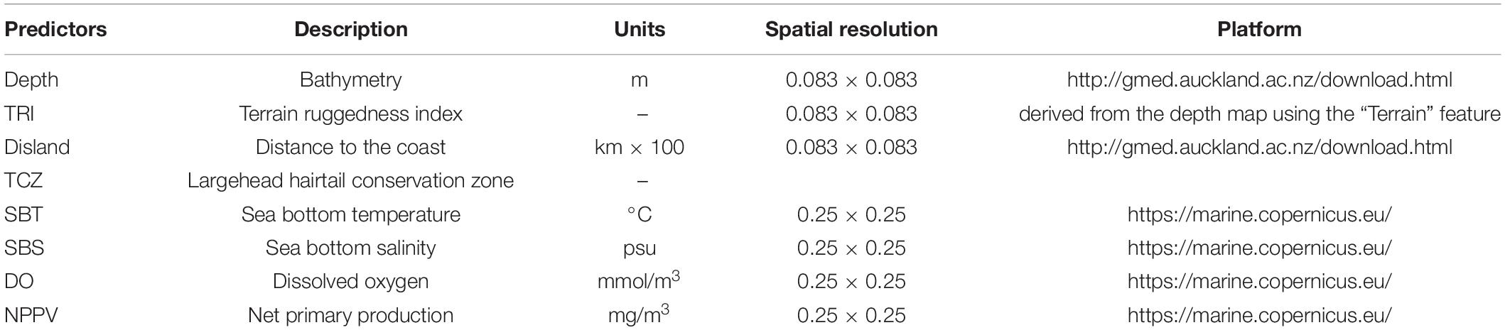
Table 1. Predictor variables used for modeling largehead hairtail juveniles.
Statistical Models
Fishery-independent surveys often overlook any species-specific specimens at unfavorable conditions, thus producing zero-inflated datasets (Martin et al., 2005). An exploratory analysis showed that largehead hairtail abundance data have high numbers of zeros, and the percentage of zeros per year was between 51.5 and 61.5%. For the Poisson generalized linear model (GLM), the counts of largehead hairtail were modeled as a function of year and environment variables. Strong spatial dependence was found in the Pearson residuals using the semi-variogram method (Supplementary Figure 3). Based on characteristics of spatial dependence and zero-inflated datasets, a two-step hierarchical Bayesian spatial model was implemented, providing the basis to account for the spatial autocorrelation, excess of zeros, and uncertainties associated with the sampling process (Pennino et al., 2019b; Abada et al., 2020). This model consisted of two parts: (i) modeling the presence/absence of the species in order to predict the probability of occurrence and (ii) modeling the conditional-to-presence abundances of the studied species to predict the probability of abundance (Abada et al., 2020). The spatially distributed occurrence was modeled using a binomial distribution with a logit link function and the conditional-to-presence abundance by a Poisson distribution with a log link function. The model specification is as shown in following equation.
Occurrence process: Zij∼Bernoulli(πij)
Abundance process: Yij∼Poisson(λij)
Where ZAP indicated zero-altered Poisson model, πij represents the probability of occurrence at location i and year j, while λij is the mean of the conditional-to-presence abundance. a(Z) and a(Y) represent the intercept of the linear predictor, Xij is the matrix of covariates, β represents the vector of the regression coefficients, and represent the spatially structured random effect of the occurrence and conditional-to-presence abundance respectively at location i, and Tj is the component of the temporal unstructured random effect at year j. A prior Gaussian distribution was assumed with a zero mean and a Matérn covariance function Q(k,τ), which depends on the hyperparameters k and τ that represent its range and variance.
The Integrated Nested Laplace Approximation (INLA) methodology and package3 were applied to obtained Bayesian parameter estimates and predictions, which were implemented in R. The INLA algorithm is a deterministic algorithm for Bayesian inference and has a greater accuracy and a shorter computing time than Markov chain Monte Carlo (MCMC) (Blangiardo and Cameletti, 2015; Lloret-Lloret et al., 2021). For the spatial effect, INLA implements the Stochastic Partial Differential Equations (SPDE) approach that involves approximating a continuously indexed Gaussian Field (GF) with a Matérn covariance function (Q) by a Gaussian Markovian Random Field (GMRF) (Fonseca et al., 2017).
Default priors (a zero-mean Gaussian prior distribution with a variance of 100) were assigned for all fixed effect parameters, which are approximations of non-informative priors and have little influence on the posterior distributions. Penalized complexity priors were assigned for the parameters of the spatial random field. The priors for the range r (the distance at which spatial autocorrelation was small) was set to r < 100 km = 0.001, meaning that the range is unlikely to be smaller than 100 km because the distance between 0 and 100 km was relatively small according to the histogram of Euclidean distance between sampling sites (Supplementary Figure 4). The reason for using the value of 0.001 in this prior was to avoid overfitting data in the spatial random field. The mesh that defined the spatial domain was created with 1220 nodes. The mesh resolution gets finer, the boundaries between the different Ω should be resolved more precisely, but increases the computational burden. We set a ratio of 1–5 between the resolutions in the inner and outer mesh, following a recommended ratio by Zuur and Ieno (2017).
Model Selection and Validation
A two-step model selection was performed by testing all possible combinations among the possible variables and spatial-temporal structure. First, the explanatory variable selection was performed beginning with all possible interaction terms using the Poisson GLM model without spatiotemporal effect to save running time. Only the best combination of variables was chosen based on the lowest Deviance Information Criterion (DIC) (Berg et al., 2004), Watanabe-Akaike information criterion (WAIC) (Watanabe, 2010). Specifically, DIC and WAIC measured the compromise between fit and parsimony in the model and were used to measure goodness-of-fit. WAIC is similar to the DIC but the effective number of parameters was computed in a different way. Preliminary analysis showed that Poisson GLM has a non-linear residuals pattern, and the non-linear Depth, SBT, and NPPV effects were identified. Thus, linear combinations on the different latent effects were defined, and their posterior marginals estimated using a smoothing splines. We chose a thin plate regression spline as the type of smoother, the smoother was fitted with 5 knots to control effective degrees of freedom and save on computational time, fitting the smoother procedure was done in “mgcv” package by using the “by” argument in the s() and smoothCon functions (Wood, 2017; Zuur and Ieno, 2017). Finally, SBS and TRI were deleted from the predictors due to high DIC and WAIC. Once the relevant predictors had been selected for the model, a series of models with different spatio-temporal effects were developed based on the selected variables of the first step. M0 was a Poisson GAM model with neither temporal effect nor spatial effect; M1 was a Poisson GAM model with spatial random field and constant over time; M2 included a spatial effect that varied annually. The models were ranked by AIC/WAIC, with the best approximating model being the one with the lowest AIC/WAIC value.
Cross-validation was applied with a 10-fold partitioning method based on randomly selected training and test data sets to assess model performance. The binomial part was tested for prediction sensitivity using the area under the receiver-operating characteristic curve (AUC). The abundance part was evaluated by comparing the predictions to the observations using Spearman’s rank correlation analysis. The correlation coefficient (r) range from –1 to 1, where those closer to 1 indicate better predictions (Pennino et al., 2019a).
Identifying Conservation Priority Areas
The spatial pattern of largehead hairtail distribution was computed by multiplying the spatial prediction for the probability of non-zero CPUE and the prediction for the positive CPUE, we simply rescaled the abundance index to obtain suitability index (SI) for each survey and cell, SI varies between 0 and 1. Using a threshold value, it was easily identified the areas of greatest concentration of juveniles, that is the hotspots of abundance. SI was computed as follows:
where A is the predicted abundance; Amin and Amax are the minimum and maximum values of the predicted abundance. Hotspots areas were identified as having SI values above 0.6. Moreover, the spatio-temporal persistence for largehead hairtail was estimated by measuring the relative persistence of cell i as a hotspots area. The index of persistence was calculated following the method of Fiorentino et al. (2003). If grid cell i was included in a hotspots area in year j, it was marked with δij = 1 and δij = 0 otherwise. Then, the spatial persistence index per cell was mapped to determine the location of priority largehead hairtail conservation areas. Ii was computed as follows:
Where n was the number of surveys considered.
Results
Binomial Component
Based on DIC and WAIC minimum criteria, the model without the spatio-temporal effect showed higher DICs, WAIC than those with this effect (Table 2). Finally, the spatial random domain model with specific years was selected (STRF), and the predictive variables included Year, Depth, Disland, TCZ, SBT, DO, and NPPV. According to the analysis results of the optimal model (Table 3), the occurrence probability and abundance of largehead hairtail showed an interannual oscillation change during 2014–2017. The occurrence probability was higher in 2015 and 2017 and the lowest in 2016. The abundance was the highest in 2016 and the lowest in 2014. Among the environmental variables of the binomial model, TCZ and Disland were found irrelevant on the variability of the largehead hairtail occurrence, while DO (posterior mean = 0.568; 95% CI = [0.4, 0.74]) showed a positive relationship with the largehead hairtail occurrence.
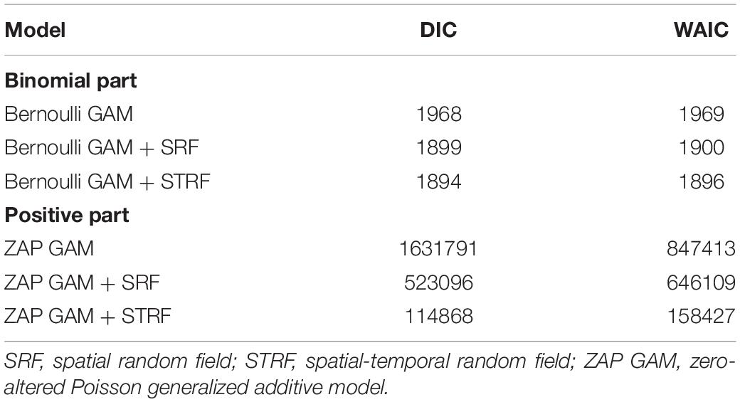
Table 2. Model comparison for the models with different spatial effects.
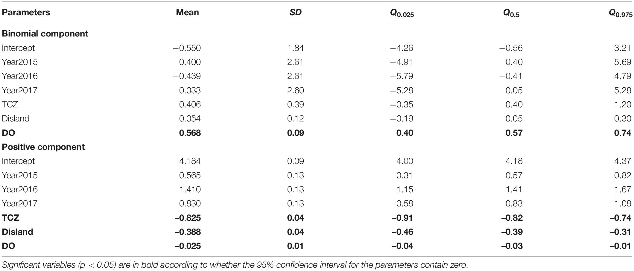
Table 3. Numerical summary of the marginal posterior distribution of the fixed effects for the Poisson GAM STRF model.
The overall predictability of the models was evaluated using the area under the receiver-operating curve (AUC). AUC was 0.81, indicating good model prediction performance and an excellent degree of discrimination between the locations with juvenile largehead hairtail presence and absence.
Depth, NPPV, and SBT returned a smooth spline, the basis functions were provided in the Supplementary Table 2. Indeed, the binomial and positive models captured the non-linear relationship between these environmental variables and response variables (Figures 2, 3). Depth showed a negative relationship with the probability of occurrence, i.e., the probability of occurrence was lower in deeper waters. SBT showed the opposite trend, with a positive effect on largehead hairtail occurrence. In particular, the probability of occurrence increased rapidly from the temperature of 10°C. However, a decreasing trend was found when SBT was above 17–18°C. The probability of occurrence showed a decreasing trend with NPPV increasing from 0 to 70 mg/m3 (Figure 3), while the probability of occurrence showed a unimodal pattern above this concentration. Finally, the probability of occurrence slowly increased and then decreased with a concentration above 140 mg/m3.
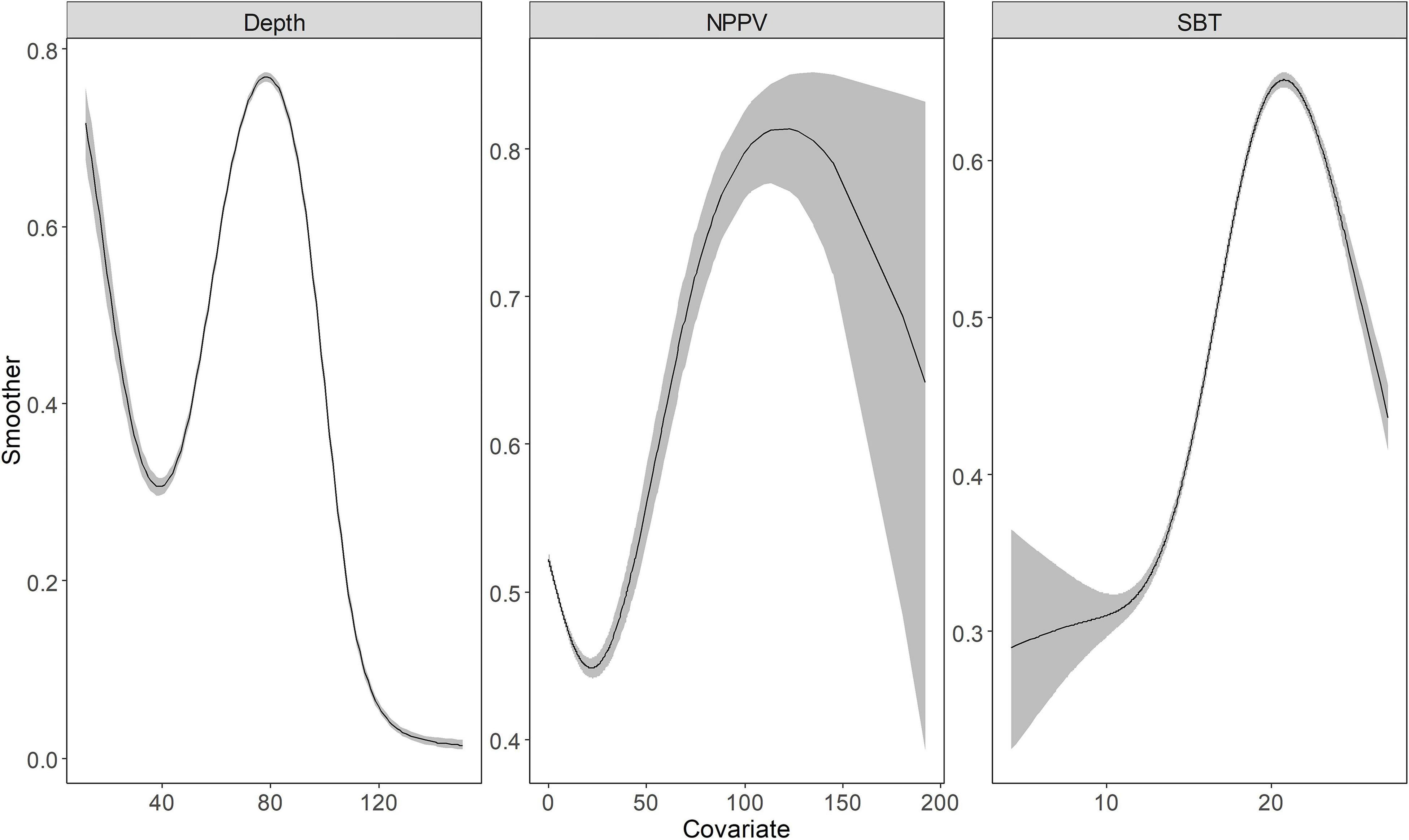
Figure 2. The functional response of Depth, Net Primary Production (NPPV), and Sea Bottom Temperature (SBT) with respect to the predicted abundance of the juvenile largehead hairtail from 2014 to 2017. The solid line represents the smooth function estimate; the shaded region represents the approximate 95% credibility interval.
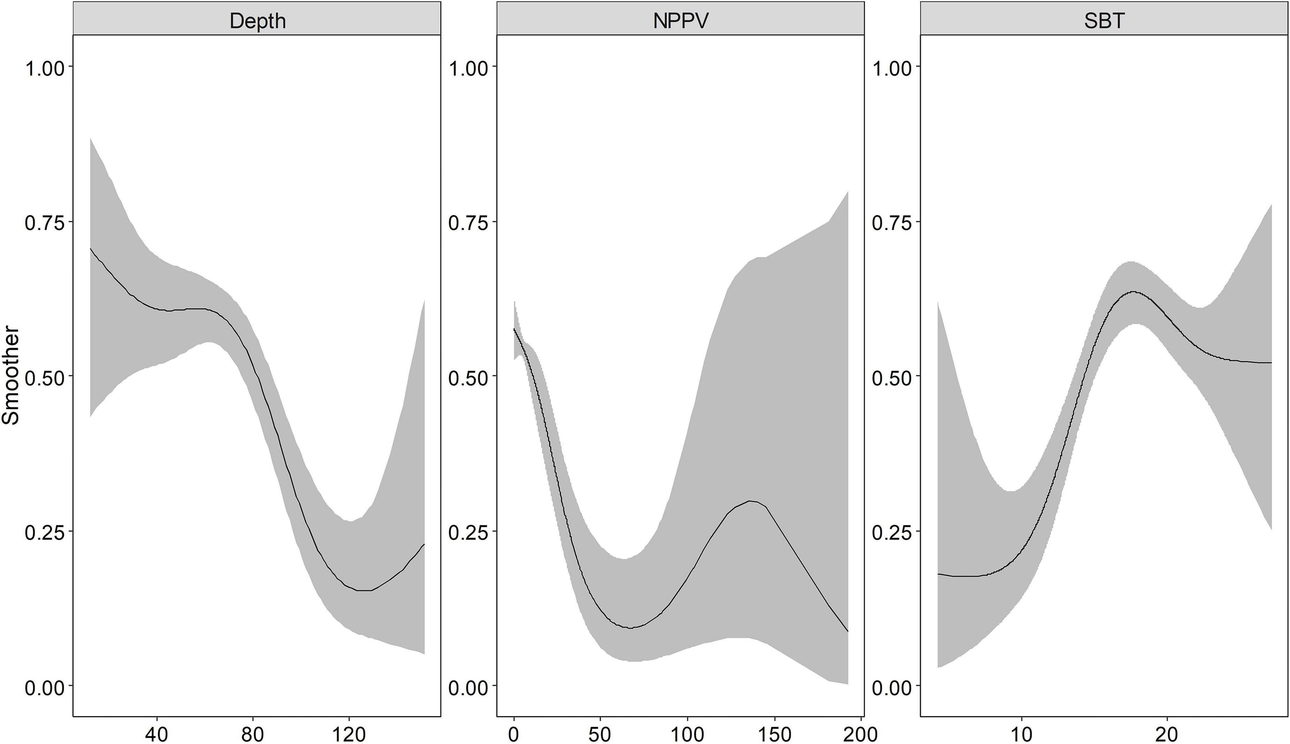
Figure 3. The functional response of Depth, Net Primary Production (NPPV), and Sea Bottom Temperature (SBT) with respect to the predicted occurrence probability of the juvenile largehead hairtail from 2014 to 2017. The solid line represents the smooth function estimate; the shaded region represents the approximate 95% credibility interval.
Both occurrence and abundance estimations were patchy, kernel smoothing method was applied to predictive data for better visualization. The mean posterior probability of largehead hairtail occurrence in the ECS showed a more coastal distribution, and higher probabilities of occurrence (above 0.5) appeared in medium-shallow waters with high bottom temperatures (Figure 4). Moreover, the probability of occurrence in the southern waters of Jeju Island was relatively higher and spread wide, but the range showed inter-annual changes, with the largest range in 2017 and the smaller range in 2014, 2015, and 2016. The map of the spatial effect showed a longitudinal pattern, with positive values in the western part and negative values in the eastern part (Figure 5).
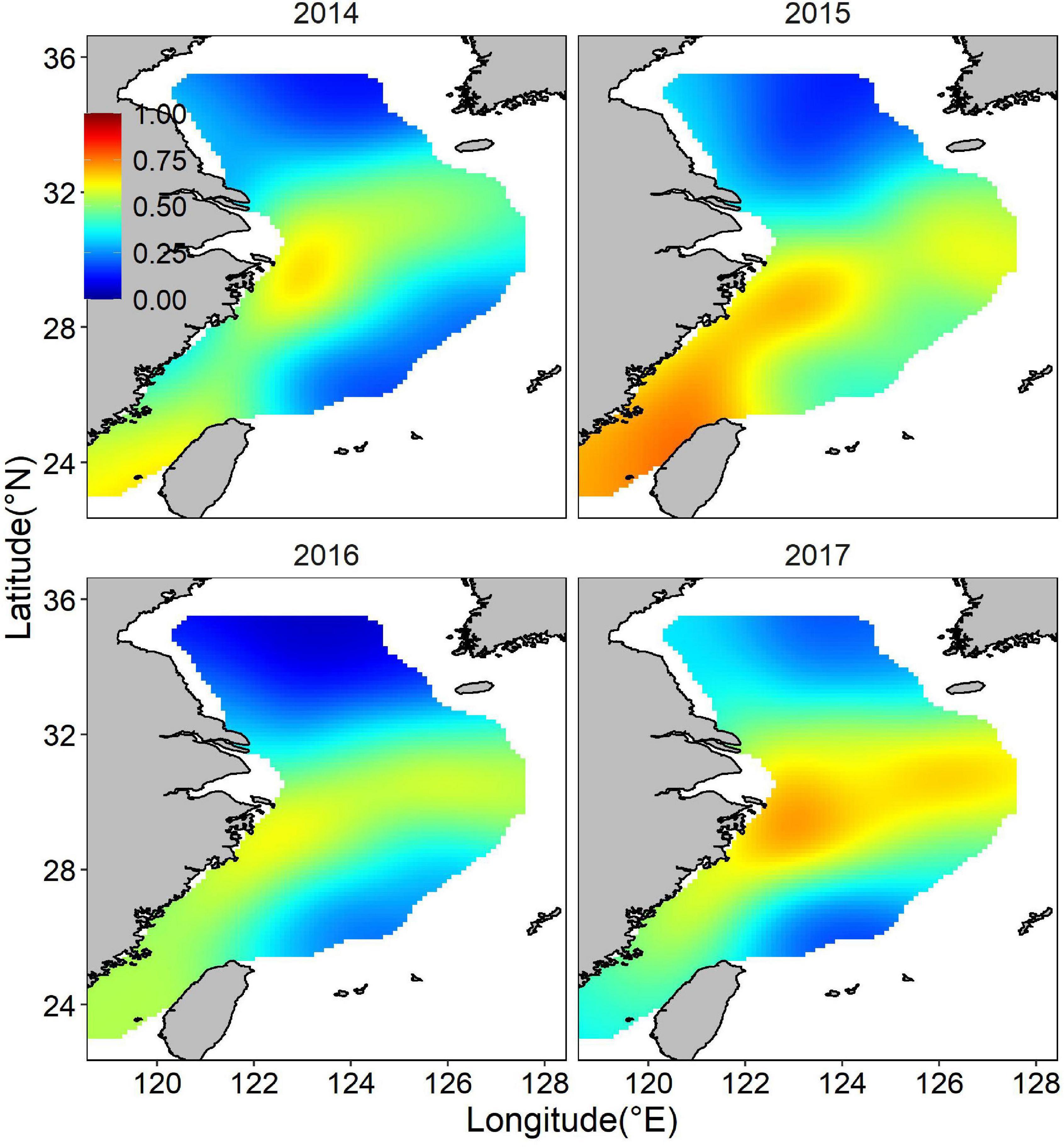
Figure 4. Distribution of the posterior mean of juvenile largehead hairtail occurrence probability from 2014 to 2017.
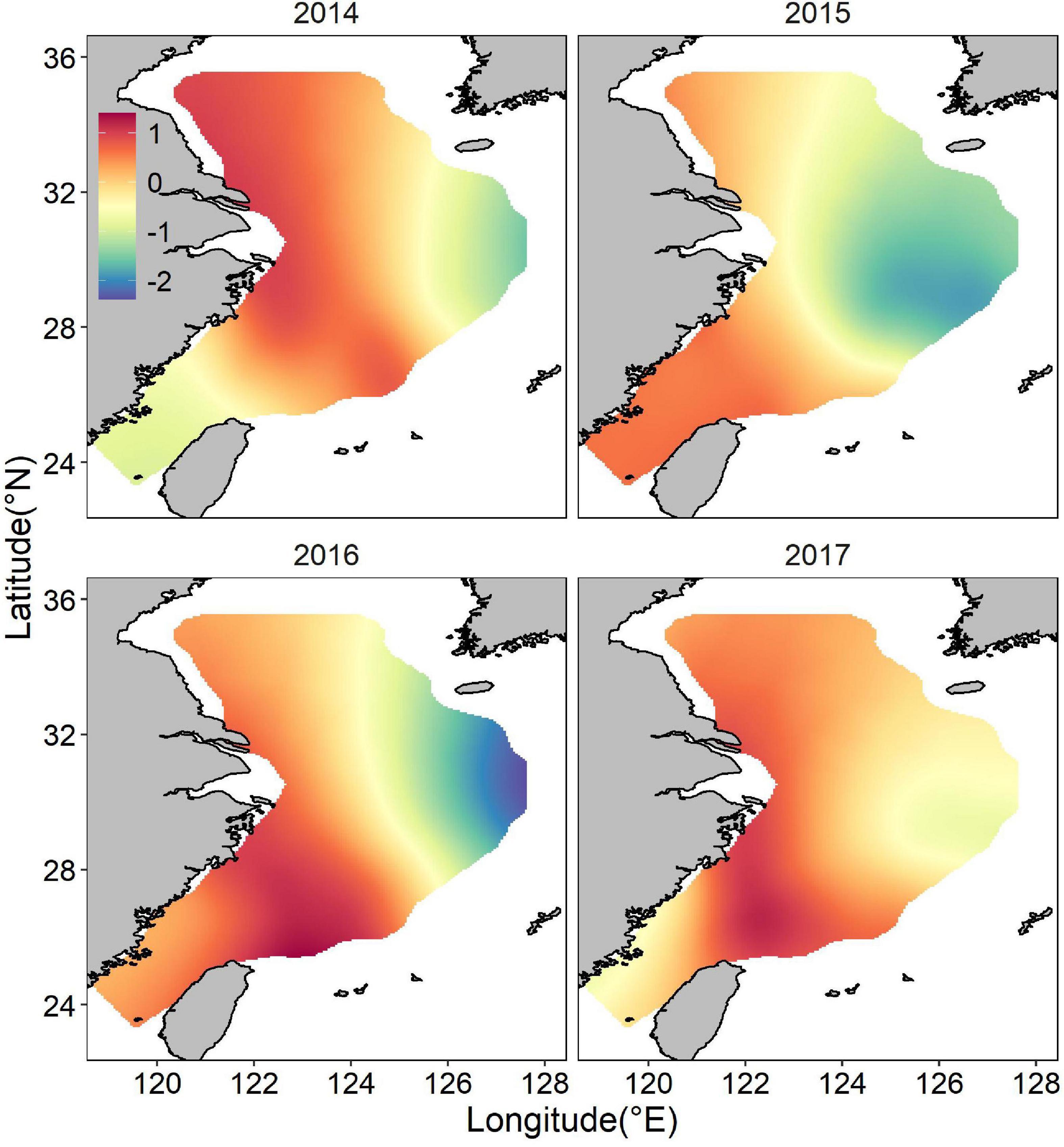
Figure 5. Distribution of the posterior mean of the spatial random effect for juvenile largehead hairtail occurrence from 2014 to 2017.
Abundance Component
According to the positive model with the best fit, Spearman’s rank correlation coefficient of r = 0.89 (n = 1658) was achieved between the observed and predicted values, indicating excellent prediction performance of the models. The abundance variability was mainly explained by TCZ, Disland, DO, Depth, NPPV, SBT, and the spatial and temporal effects (Table 3). The results showed a negative relationship between TCZ (posterior mean = –0.825; 95% CI = [–0.91, –0.74]), Disland (posterior mean = –0.388; 95% CI = [–0.46, –0.31]), DO (posterior mean = –0.025; 95% CI = [–0.04, –0.01]) and the largehead hairtail abundance. Depth, NPPV, and SBT were retained variables that required smoothing splines (Supplementary Table 2). The abundance of the largehead hairtail decreased on the inner shelf until 40 m, increased in middle depth water, and declined in deeper water. SBT and NPPV had similar effects on abundance, showing a unimodal pattern of first increasing and then decreasing. Results showed higher abundances in waters between 60 and 90 m, with SBT between 19 and 23°C and NPPV higher than 50 mg/m3 (Figure 2).
The posterior mean of largehead hairtail abundance showed a heterogeneous spatial pattern (Figure 6), highlighting two hotspots: one along the coast of Zhejiang Province and the other at the Fujian coast. The identified hotspots overlapped partially with largehead hairtail spawning stocks reserve and TCZ. Other smaller areas with high abundance were in offshore waters of northern Zhejiang Province in the high-temperature areas. These hotspots showed the characteristics of scattered patch distribution. Although the abundance had similar spatial distribution in different years, the location and range of high abundance also showed changes in specific years, especially in the southern ECS. In 2014 and 2016, high abundance areas concentrated around the coastal waters and expanded northward. High abundance areas occupied all the coast of the Fujian Province in 2017. In 2015, the high abundance locations remained unchanged but expanded up to the offshore waters of ECS. The map of the spatial effect showed a latitudinal gradient, with positive values in the southern part, sporadic area that showed negative values (Figure 7).
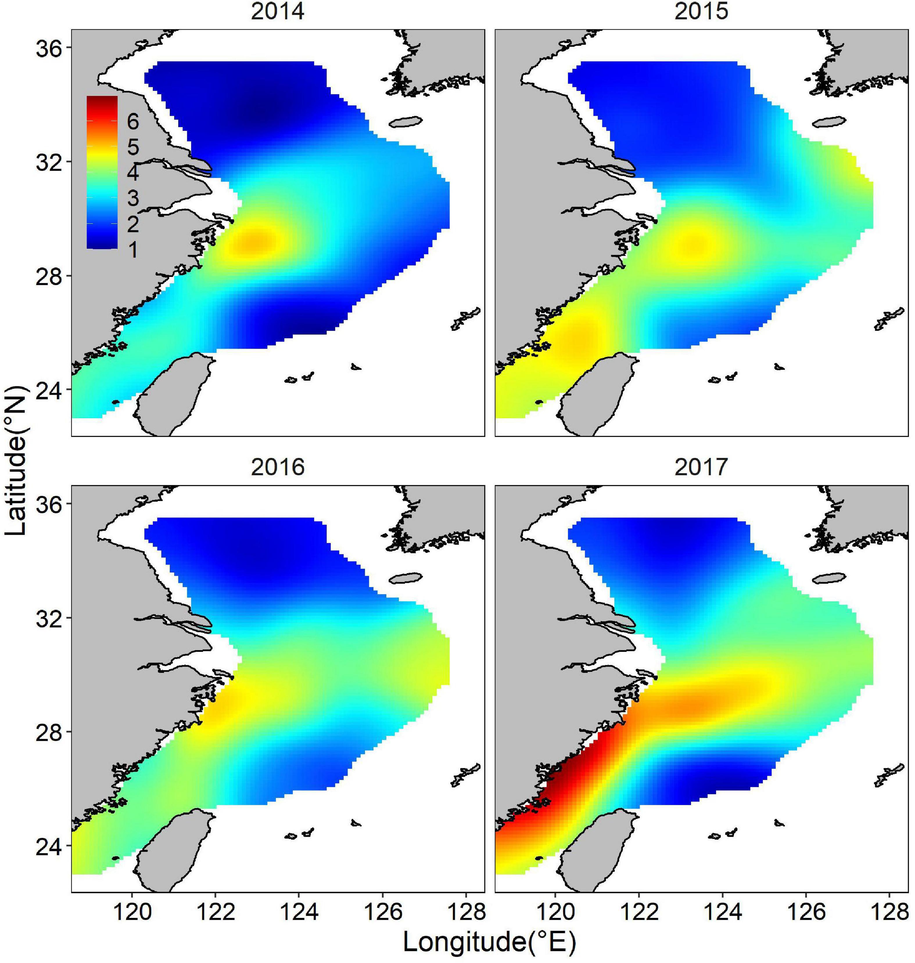
Figure 6. Distribution of the posterior mean of juvenile largehead hairtail abundance (natural logarithm) from 2014 to 2017.
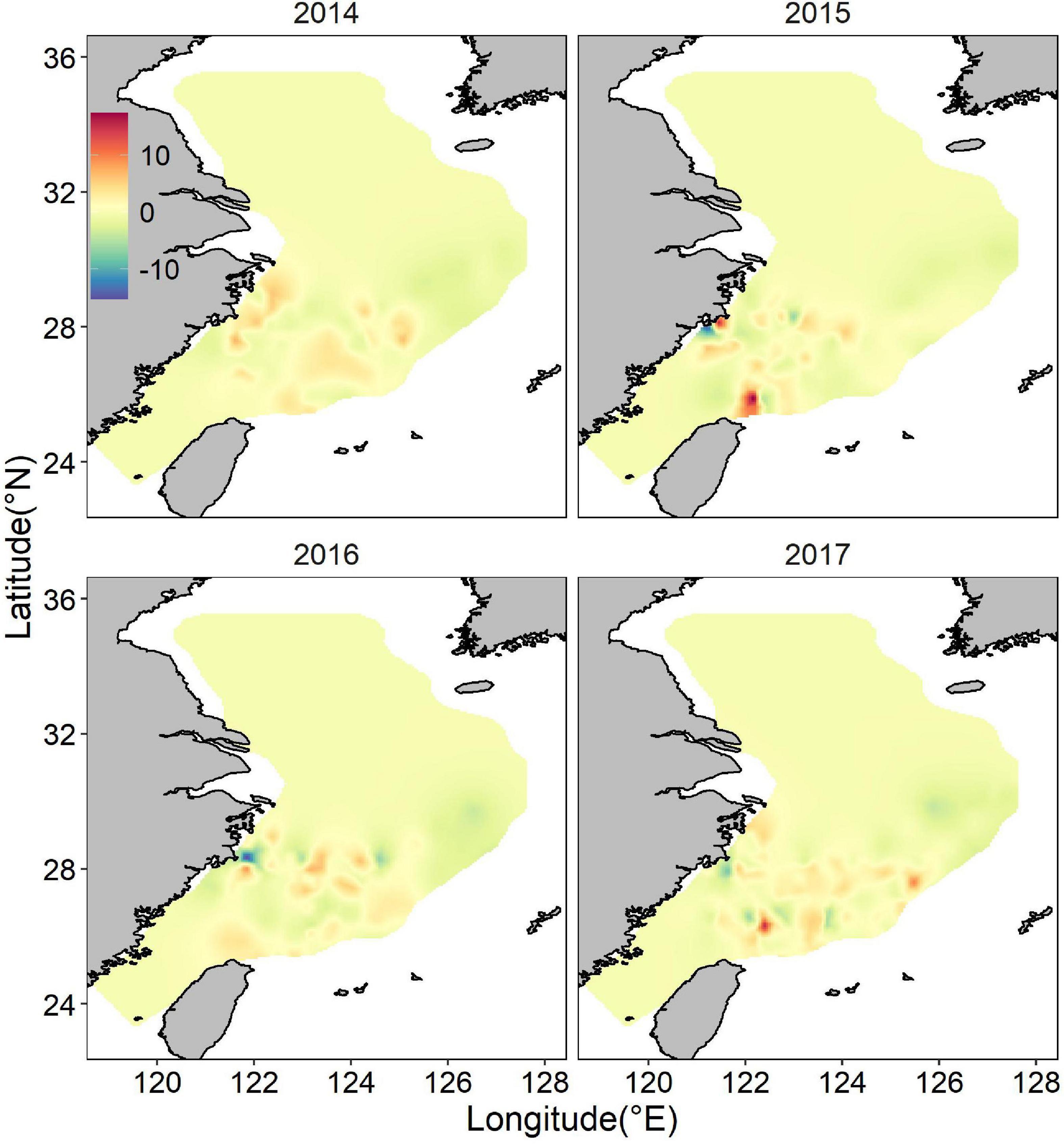
Figure 7. Distribution of the posterior mean of the spatial random effect for juvenile largehead hairtail abundance from 2014 to 2017.
The occurrence probability and abundance inside the protected area were higher than those outside the protected area (Figures 8A,B), and the inter-annual difference reached significant levels, indicating that the protected area concentrated on higher occurrence frequency and abundance. The probability of occurrence and abundance in the protected areas were relatively higher in 2014 and 2017 but lower in 2015 and 2016. The occurrence probability and abundance varied within a narrow range outside the reserves than those inside the reserves. The median value of occurrence probability ranged from 0.40 to 0.48 and the median value of logarithmic transformation abundance ranged from 0.69 to 1 outside the TCZ, the performance of both models were stable over time, indicating that both models captured relevant spatial environment relationships outside the TCZ over time.
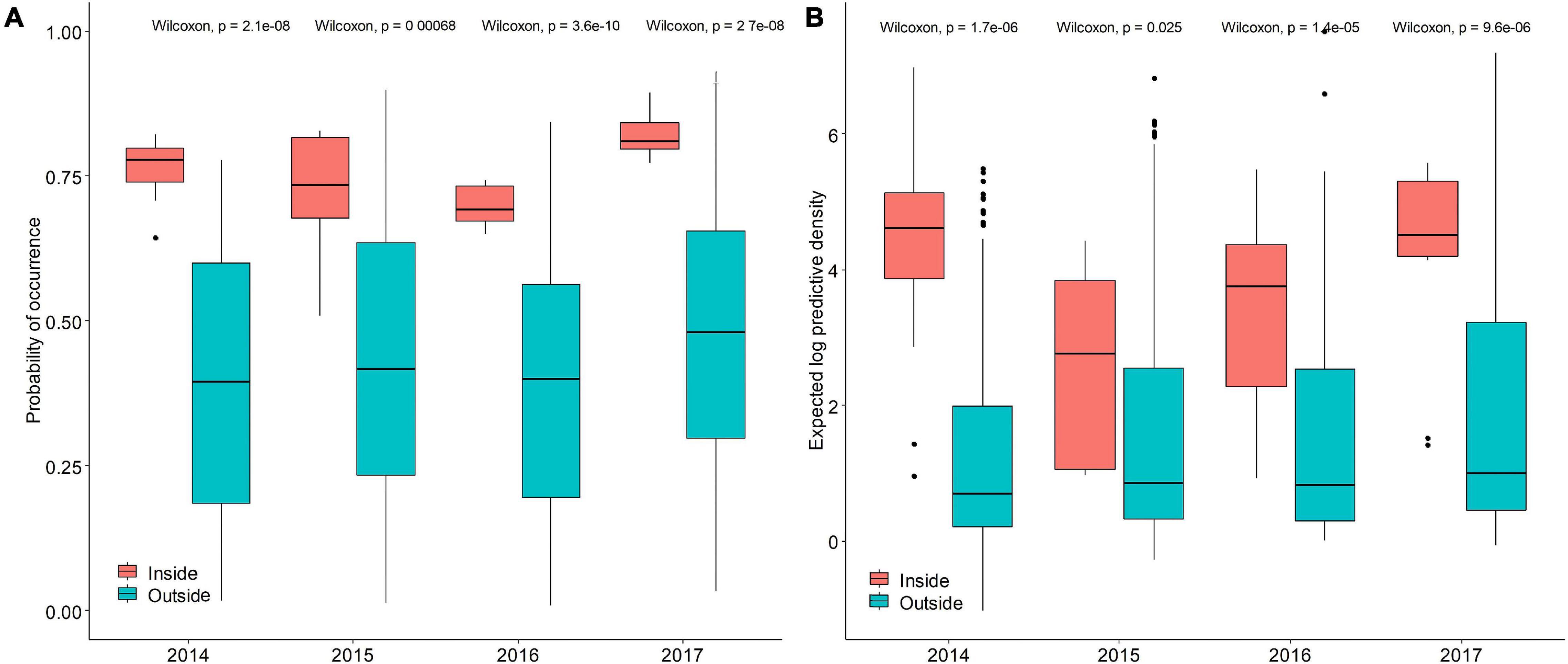
Figure 8. The predictive performance boxplots of the (A) binomial and (B) positive components of the Poisson GAM STRF model. Red boxes represent survey area inside the TCZ, blue box represent survey area outside the TCZ.
Priority Area Identification
The abundance distribution of the posterior mean combined by binomial and positive components showed a similar spatial pattern with only the abundance component (Figure 9), which showed a consistent spatial distribution pattern both of binomial and positive components. The spatial and temporal stability of hotspots were considered a useful measure to evaluate their suitability as nurseries. The larger nursery areas (I > = 0.75) under hotspots cutoff value of 0.6 appeared sporadically along the coast of mainland China. At least three persistent areas were identified. A large persistent area was on the right edge of TCZ, most of which was not in the TCZ. The smaller persistent areas were 122 km off the TCZ. Persistent nurseries covered 2.86% of the study area and included approximately 16% of juvenile largehead hairtail (Figure 10). When the hotspot threshold was set at 0.7, only one persistence area was identified, which was closed to but outside the TCZ (Figure 10).
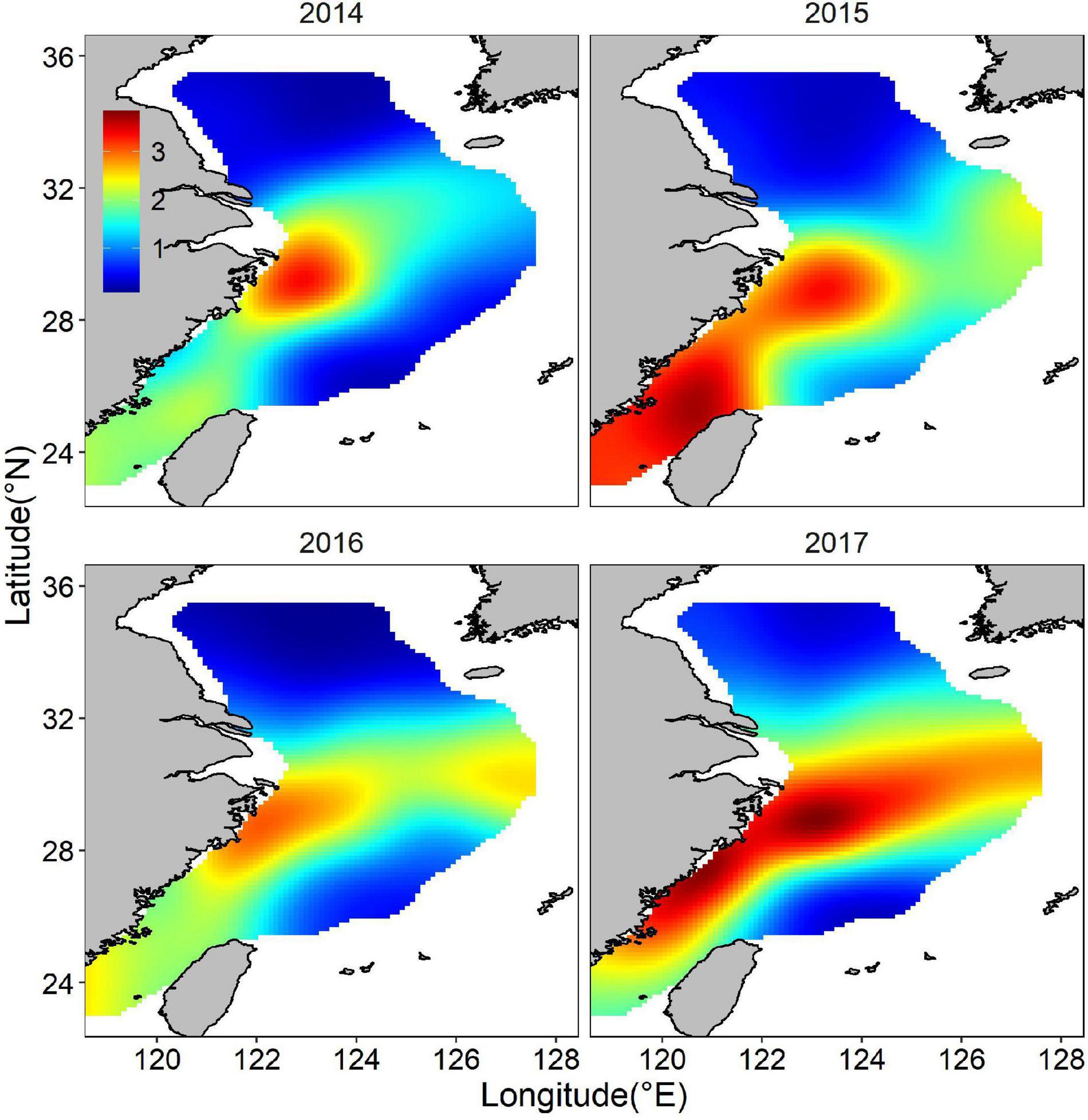
Figure 9. Abundance distribution (natural logarithm) of the posterior mean combined by binomial and positive components for juvenile largehead hairtail from 2014 to 2017.
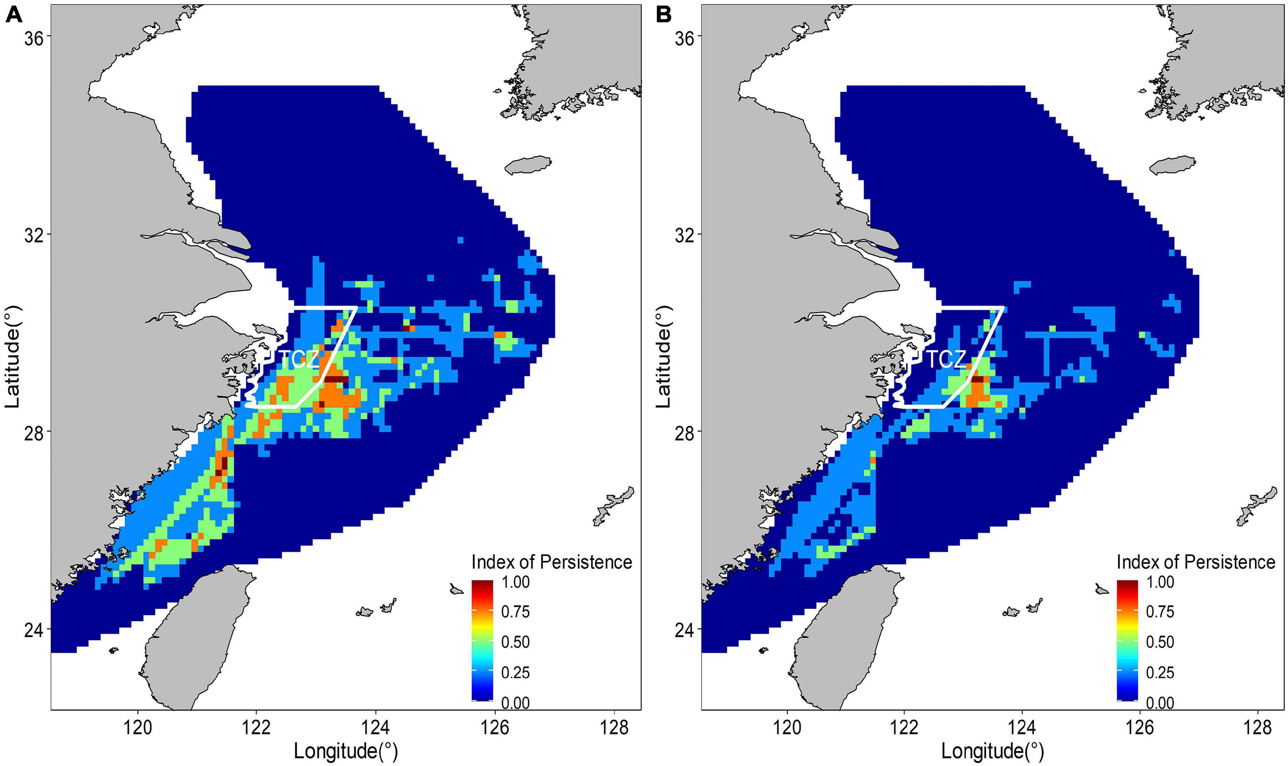
Figure 10. Temporal persistence of nurseries hotspots estimated by suitability index above 0.6 (A) and suitability index above 0.7 (B) from 2014 to 2017.
Discussion
The red line for ecological protection marks the minimum ecological protection space designated by the Chinese government based on the requirements for protecting the integrity and connectivity of the ecosystem so as to maintain regional ecological security and sustainable development (Xu et al., 2015; Lin et al., 2016). Protecting sensitive ecosystems and important ecological functions is an important element of the red line for ecological protection. Marine fish spawning grounds and nursery grounds are important for replenishing the stock and maintaining biodiversity, while non-selective fishing often leads to massive bycatch of juveniles. Therefore, conserving nursery grounds is important for the sustainable development of fisheries resources, and the spatial characteristics of key habitats for exploited stocks need to be understood. Thus, identifying the spatio-temporal distribution of nursery grounds is a prerequisite for setting the red line of ecological protection. In this paper, nursery grounds were identified based on the persistence of the hotspots of the juveniles spatial distribution. Specifically, two spatio-temporal structure models were adopted to represent the juveniles’ occurrence and abundance, which were combined to present the hotspots, and the persistence index was used to map the spatial distribution of nursery grounds. This method of using abundance distributions to determine nursery grounds is particularly suitable when the contribution of nursery grounds to the adult stock and the ecological processes are unclear (Beck et al., 2001; Gillanders et al., 2003; Maynou et al., 2003; Tserpes et al., 2008; Garofalo et al., 2011; Colloca et al., 2015; Paradinas et al., 2015). Many researches focused on identifying the nursery grounds by developing different metrics (Colloca et al., 2009, 2015). Geostatistical techniques are often adopted in identifying the nursery grounds of fish species such as red mullet, European hake, and deep-water rose shrimp in the southern Adriatic Sea (Carlucci et al., 2009), as well as European hake nursery grounds in the central Mediterranean Sea (Colloca et al., 2009). Colloca et al. (2015) argued that using unique standardized method of spatial modeling for all species/stages/areas was unfeasible due to the large observed differences in the availability of data and causal mechanisms. Colloca et al. (2015) adopted adaptive methods for different species to overcome the issues of autocorrelation, non-linearity and large amount of zero catch. In this study, we used the ZAP models to deal with zero inflated data, that was similar to the zero inflated generalized additive models adopted by Colloca et al. (2015). In addition, alternative Bayesian spatio-temporal models were fitted using INLA-SPDE approach, and we selected the most appropriate model that captured spatial and temporal effects, which explained additional sources of uncertainty on the structure of dependence, thus was able to accurately describe the spatial distribution of nursery grounds. In this case, areas of high abundance but low probability of occurrence may not be considered important nursery habitats. Instead, only locations of high abundance and high probability of occurrence are identified as the cores of nursery grounds. In this study, the concepts of habitat suitability index and hotspots were used to identify core areas of nursery grounds (Colloca et al., 2015). Specifically, hotspots were identified by a suitability index standardized between 0 and 1, which were then classified into important nursery grounds using different thresholds. In this way, the spatial distribution of nursery grounds can be more flexibly compared under the same scale, making it possible to distinguish whether there are unique spatial processes or whether the spatial structure has changed over time. Compared to the geostatistical aggregation curve (Colloca et al., 2009; Tamdrari et al., 2010) or the Getis-Ord hotspot analysis (Colloca et al., 2015; Zacher et al., 2018; Milisenda et al., 2021), the suitability index analysis does not require complex calculation but lacks statistical interpretations and objectivity in the hotspot classification criteria. In this study, since the spatial distribution pattern of juvenile largehead hairtail was inter-annually stable with slight variations in the southern part of the ECS, the persistence index could be used for nursery grounds identification. In addition, two thresholds were used to identify important nursery grounds based on different aggregation intensities.
Due to the presence of permanent largehead hairtail nursery grounds in the study area, different thresholds were adopted in the classification of nursery grounds hotspots so that the importance of different areas can be evaluated. Three permanent nursery grounds were identified under a suitability index of 0.6, and the two larger ones were in the waters of Taizhou Islands and the eastern waters of Yushan Island, both of which had relatively high abundance and probability of occurrence. Parts of the two nursery grounds were inside the TCZ, which was established for the exclusive protection of largehead hairtail, especially the spawning stock and juveniles. The TCZ is rich in feedstuff organisms, and trawling is prohibited from April to September, which provides a stable and high-quality ecosystem for juvenile largehead hairtail and improves their survival rate. However, parts of the two nursery grounds were still not within the TCZ. The smallest nursery ground was in the southern waters of the Beijishan Islands and Nanjishan Islands. Although the abundance of the smallest nursery ground was lower than those of the two northern nursery grounds, the location of the core area is stable, and its abundance was even higher in specific year. Since 2017, the area has been managed under the local government’s spawning ground protection policy and is protected from any fishing operations other than longline fishing from April to August each year. The permanent nursery grounds were extremely small and outside the TCZ under a suitability index of 0.7, which may be related to the life history stage of the population. Since the TCZ was set up to protect the spawning stock and juveniles, the juveniles could be transported to the shallow nearshore waters and feeding around (Wu, 1991). The juvenile largehead hairtail in our study were mainly immature individuals under 20 g (123 mm). They have migratory ability and move across TCZ for seeking feedstuff around the spawning grounds, which is also a common behavior of many fish species.
Functional response curves are important for understanding the optimal environmental adaptability and tolerance of a certain species as they provide information on how species respond to environmental gradients. The range of environmental features for potential juvenile largehead hairtail habitats was obtained based on the findings in this study. The occurrence and abundance distribution of juvenile largehead hairtail were closely related to water depth and hydrological conditions. The abundance distribution showed optimum areas within the depth range from 60 to 100 m with a turning point at 80 m. Abundance was positively correlated with water depth in the range of 40–80 m and negatively correlated with water depth above 80 m. Beyond 60 m, the probability of occurrence was negatively correlated with water depth, i.e., the probability of occurrence was higher in shallow waters within the depth of 60 m. Although the probability of occurrence was greatest in shallow waters at 40 m, there was a high uncertainty due to the limited number of shallow water survey stations with depths smaller than 40 m. The inconsistency between the optimum occurrence areas and the peak abundance areas may be attributed to individuals’ choice of different habitats for their development, i.e., the ecological niche differentiation of different sized individuals drives the adaptation of occurrence and abundance to local areas. The differences in occurrence and abundance were adjusted through the competition for resources, which, in turn, drives the migrations between different areas (Bijleveld et al., 2018). In macroecology, different mechanisms have been proposed to explain the interspecific abundance-occurrence relationships. The ecologically based explanations focus on the availability and distribution of habitat and food resources, individual size and the corresponding migration ability, species specificity, and adaptation to the habitat (Borregaard and Rahbek, 2010; Miranda and Killgore, 2019). As in the description of macrobenthos in the Wadden Sea made by Bijleveld et al. (2018), there is no general relationship between the biomass of a species and its occupancy. Friedland et al. (2021) studied the interannual variation in the occurrence and biomass gravity center of fish and macroinvertebrates in the northeastern U.S. shelf ecosystem and found that habitats differed in depth and that habitats with the center of gravity were in shallower waters and the biomass gravity center was shifting to deeper waters. Since the occurrence and abundance characteristics of species distribution offered valuable information for the management process but showed inconsistent patterns, occurrence and abundance distributions need to be balanced in the spatial planning of resources.
Thermal conditions constrain species’s distributions through physiological processes (Stuart-Smith et al., 2017). All fish species are characterized by their temperature tolerance and the preferred temperature in which they demonstrate optimal growth (Kır et al., 2017). Juveniles are expected to be adapted to a relatively narrow range of temperatures due to relatively weak thermal tolerance (Turko et al., 2020). Both the occurrence and abundance of juvenile largehead hairtail showed optimal temperature ranges, juveniles showed a preference for warmer waters to colder waters, confirming previous studies (Mi, 1997; Wang et al., 2011) that suggested that warmer waters promoted largehead hairtail growth. The results in the present study indicated a narrower temperature range of the bottom water temperature than that was reported by You and Xu (1984), which was 16–22°C in summer in the central fishing ground. Our results suggested that adult and juvenile largehead hairtail inhabited a similar thermal niche, but juveniles that occupied nursery grounds were restricted to these habitats because of narrower physiological thermal tolerance compared to tolerances of adults. Sun et al. (2020b) studied daily growth of young-of-the-year largehead hairtail by otolith microstructure analysis, suggested that daily growth of juvenile largehead hairtail was influenced by the interactive effects of water temperature and nutrient supplies. For the October-spawned and November-spawned cohort, otolith daily increment showed maximum growth at temperatures 18 and 21°C, respectively, which were approximate optimal temperature in the nursery areas of our present study. Temperature-dependent physiological mechanism may contribute to persistent existence of largehead hairtail nursery grounds. However, the mechanism of the effects of increased thermal variability on largehead hairtail physiology and stress are not well understood, many experimentally manipulated thermal regimes and found that thermal variance affected the biochemical reaction rates and metabolic rates of fish species (Brown et al., 2004; Steel et al., 2012). Moreover, the formation of largehead hairtail nursery grounds may largely depend on those that maximize a particular physiological performance, but will also depend on food and habitat availability and various other ecological factors (Payne et al., 2015).
Largehead hairtail spawn almost year round with peak spawning periods spanning from April to October in the East China Sea. In late spring, the spawning stock migrates from the southern Zhejiang offshore to the northern Zhejiang offshore drove by the Taiwan warm current (TWC). In autumn, the spawning stock spawns offshore at the mouth of the Yangtze River and gradually migrates southward (Li, 1982). The waters around the nursery grounds and spawning grounds are dominated by two current systems with different features, i.e., the low-temperature water along the coast of Jiangsu and Zhejiang in nearshore areas, and the high-temperature water of the TWC in offshore areas. Thus the primary productivity is high in the frontal zone (Jiao et al., 1998). The location of nursery grounds changes with the advance and retreat of the Taiwan warm current. As the temperature decreases, the aggregation area of largehead hairtail moves south; as the temperature increases, the aggregation area moves north. The catch of largehead hairtail is also closely related to the coastal current and the TWC. When the coastal current is stronger, the catch in the ECS is higher, and vice versa. The catch in the ECS is inversely proportional to the strength of the TWC (Chen et al., 2004). The effects of coastal current and the TWC on catch may be related to the transport and survival rate of juvenile largehead hairtail. TWC originating from the northward Kuroshio flows along the Sea of ECS coast, has poor nutrients and low primary production (Yatsu et al., 2013; Karu et al., 2020). In contrast, the coastal current has rich nutrients and high primary productivity (Ichikawa and Beardsley, 2002). In some years, strong TWC and weak coastal current can change the nursery grounds location of largehead hairtail, and the quality of largehead hairtail nursery grounds declines, thus reducing the early survival rate. The effects of NPPV are consistent with those of temperature on the abundance. Increases in temperature within a certain range promote increases in primary productivity. Guan et al. (2014) describes the relationship between the maximum photosynthetic rate and temperature exhibits a peak near 20°C, followed by a decline with further increases in temperature through the VGPM (Vertically Generalized Production Model) algorithm, indicating that although higher temperature usually increased photosynthesis, it was often associated with the nutrient limitation that inhibited phytoplankton growth. In addition, increasing temperature can increase the respiration of phytoplankton and limit the accumulation of photosynthetic products. Although the relationship between temperature and NPPV was not analyzed in this paper, we found the abundance of juvenile fish began to decrease at temperatures above 20°C and NPPV above 120 mg/m3, which shown a similar response trend. Du et al. (2020) concluded that low salinity and high temperature were conducive to the growth of phytoplankton, which promote the migration, feeding, aggregation of largehead hairtail, and the formation of fishing grounds in the ECS.
The non-linear relationship between NPPV and the abundance of juvenile largehead hairtail showed that the effect of NPPV on the abundance was positive over a wide range but shifted to negative beyond a threshold. Guan et al. (2014) found the same pattern in the relationship between Scomber japonicus and NPPV in the ECS and concluded that interspecific competition between Scomber japonicus and largehead hairtail limited the biomass increase of Scomber japonicus. In addition, a negative feedback mechanism exists between zooplankton and phytoplankton (Goldyn and Kowalczewska-Madura, 2008; Daewel et al., 2014; Vallina et al., 2014). As a result, the abundance of zooplankton decreases with the increases in NPPV. Thus the abundance of zooplankton-feeding fish is regulated through the bottom-up mechanism. Juvenile largehead hairtail mainly feed on plankton and small pelagic fish (Zhang, 2004), thus having a closer trophic relationship to the NPPV. Chen et al. (2004) analyzed the relationship between the feedstuff and fishing grounds location of largehead hairtail in the ECS using the distribution data of zooplankton from 1960 to 1981, and found that the distribution of zooplankton biomass, particularly krill was closely related to the changes of largehead hairtail fishing ground location and the migration of fish schools. However, largehead hairtail is highly cannibalistic during its juvenile and adult stages, and the weight of juvenile largehead hairtail could reach 25.2% of their stomach contents (Liu et al., 2009b). Based on the available results, the non-linear response of juvenile largehead hairtail to NPPV may be attributed to the complex ecosystems, and it is difficult to determine which mechanism controls the dynamics of juvenile largehead hairtail abundance.
Marine spatial planning is an important tool for marine fisheries management and an important means to govern marine space and promote sustainable use of marine fisheries. Currently, the understanding of the spatial ecology of marine species is limited, which is necessary for the conservation of marine species and the development of marine spatial planning approaches. As tools to support management and conservation, habitat suitability models could help identify priority conservation and management areas. This study extends the knowledge of the relationship between juvenile and the environment in the highly exploited species of largehead hairtail. Considering the commercial and economic importance of the species, the results of our present study provided priority conservation areas for permanent nursery grounds in early life history stages and that can be used to achieve sustainable and adaptive fisheries management and spatial management of human activities.
The small size and proximity of the identified permanent nursery grounds and the fact that they did not cover multiple administrative units brought the feasibility of implementing effective marine spatial planning and connected conservation area networks. Marine conservation areas are set up to manage human activities rather than fish or biodiversity. Since fishing is the most important human activity, and the distribution of trawl fishing grounds is highly overlapping with nursery grounds (Zhang et al., 2016). Thus, resistance to spatial planning stems mainly from fisheries actions, especially trawling. The smaller area of permanent nursery grounds may be a convenient feature, which could help the negotiation with fishery administrations and reducing the impacts on fisheries and fishermen (Paradinas et al., 2015). An effective assessment of permanent nursery grounds should include the spatial and temporal dynamics of the species throughout the year (Crowdera and Norse, 2008; Paradinas et al., 2015), even involving the knowledge on environmental regimes. Therefore, future studies may focus on the analysis of the spatial distribution of different months and supplement other information, such as the fishery-dependent catch and fishing effort. If a persistent pattern exists throughout the year, a permanent fishery restriction area may be recommended. However, fish reproduction is seasonal and cyclical, and concentrating on protecting the space of peak reproductive and nursery periods could prove a more flexible management approach. In addition to strict protection of existing fish distribution hotspots, new suitable habitats could be added to expand the range of hotspots. For example, analysis in this study showed potentially suitable areas were outside the permanent nursery habitats. Although most of them were at the periphery of the hotspots, those areas were even the core of distribution in specific years. At present, those potentially suitable areas are disturbed by human activities and lack of adequate protection. Due to the complex system behavior of marine populations and ecosystems, there is no guarantee that removing the stresses will lead to population recovery at times of populations decline. Therefore, precautionary action is a more robust management strategy than restoration measures under population collapse.
Data Availability Statement
The raw data supporting the conclusions of this article will be made available by the authors, without undue reservation.
Ethics Statement
Ethical review and approval was not required for the animal study because all the fish samples were collected by scientific investigation and no specific licenses for the studied populations were needed.
Author Contributions
ZL, YJ, and LLY conceived and designed the study. ZL, YZ, HZ, and CS collected the data. ZL, YJ, and LLY analyzed the data. ZL, YJ, LPY, LLY, and JC developed the initial version of the manuscript. All authors contributed to the article and approved the submitted version.
Funding
This work was supported by the National Key Research and Development Project (2020YFD0900804), Shanghai Sailing Program (18YF1429800), Special funds for survey of offshore fishery resources by the Ministry of Agriculture and Rural Affairs (125C0505).
Conflict of Interest
The authors declare that the research was conducted in the absence of any commercial or financial relationships that could be construed as a potential conflict of interest.
Publisher’s Note
All claims expressed in this article are solely those of the authors and do not necessarily represent those of their affiliated organizations, or those of the publisher, the editors and the reviewers. Any product that may be evaluated in this article, or claim that may be made by its manufacturer, is not guaranteed or endorsed by the publisher.
Acknowledgments
We are grateful to Copernicus Marine Service and University of Auckland for providing us with the marine data.
Supplementary Material
The Supplementary Material for this article can be found online at: https://www.frontiersin.org/articles/10.3389/fmars.2021.779144/full#supplementary-material
Footnotes
References
Abada, E., Penninoa, M. G., Valeiras, J., Vilela, R., Bellido, J. M., Punzón, A., et al. (2020). Integrating spatial management measures into fisheries: the Lepidorhombus spp. case study. Mar. Policy 116:103739. doi: 10.1016/j.marpol.2019.103739
Albuquerque, F., and Beier, P. (2015a). Global patterns and environmental correlates of high-priority conservation areas for vertebrates. J. Biogeogr. 42, 1397–1405. doi: 10.1111/jbi.12498
Albuquerque, F., and Beier, P. (2015b). Using abiotic variables to predict importance of sites for species representation. Conserv. Biol. 29, 1390–1400. doi: 10.1111/cobi.12520
Armstrong, J. B., Fullerton, A. H., Jordan, C. E., Ebersole, J. L., Bellmore, J. R., Arismendi, I., et al. (2021). The importance of warm habitat to the growth regime of cold-water fishes. Nat. Clim. Chang. 11:354–361. doi: 10.1038/s41558-021-00994-y
Austin, M. (2007). Species distribution models and ecological theory: a critical assessment and some possible new approaches. Ecol Modell. 200, 1–19. doi: 10.1016/j.ecolmodel.2006.07.005
Bashevkin, S. M., Dibble, C. D., Dunn, R. P., Hollarsmith, J. A., Ng, G., Satterthwaite, E. V., et al. (2020). Larval dispersal in a changing ocean with an emphasis on upwelling regions. Ecosphere 11:e03015. doi: 10.1002/ecs2.3015
Bateman, B. L., VanDerWal, J., Williams, S. E., and Johnson, C. N. (2012). Biotic interactions influence the projected distribution of a specialist mammal under climate change. Divers. Distrib. 18, 861–872. doi: 10.1111/j.1472-4642.2012.00922.x
Beck, M. W., Heck, K. L., Able, K. W., Childers, D. L., Eggleston, D. B., Gillanders, B. M., et al. (2001). The identification, conservation, and management of estuarine and marine nurseries for fish and invertebrates. A better understanding of the habitats that serve as nurseries for marine species and the factors that create site-specific variability in nursery quality will improve conservation and management of these areas. BioScience 51, 633–641.
Berg, A., Meyer, R., and Yu, J. (2004). Deviance information criterion for comparing stochastic volatility models. J. Bus. Econ. Stat. 22, 107–120. doi: 10.1198/073500103288619430
Bijleveld, A. I., Compton, T. J., Klunder, L., Holthuijsen, S., Horn, J., and Koolhaas, A. (2018). Presence-absence of marine macrozoobenthos does not generally predict abundance and biomass. Sci. Rep. 8:3039. doi: 10.1038/s41598-018-21285-1
Blangiardo, M., and Cameletti, M. (2015). Spatial and Spatio-Temporal Bayesian Models with R-INLA. New York, NY: John Wiley Press.
Borregaard, M. K., and Rahbek, C. (2010). Causality of the relationship between geographic distribution and species abundance. Q. Rev. Biol. 85, 3–25. doi: 10.1086/650265
Brennan, C. E., Blanchard, H., and Fennel, K. (2016). Putting temperature and oxygen thresholds of marine animals in context of environmental change: a regional perspective for the Scotian shelf and Gulf of St. Lawrence. PLoS One 11:e0167411. doi: 10.1371/journal.pone.0167411
Britten, G. L., Dowd, M., and Worm, B. (2016). Changing recruitment capacity in global fish stocks. Proc. Natl. Acad. Sci. U.S.A. 113, 134–139. doi: 10.1073/pnas.1504709112
Brown, J. H., Gillooly, J. F., Allen, A. P., Savage, V. M., and West, G. B. (2004). Toward a metabolic theory of ecology. Ecology 85, 1771–1789. doi: 10.1890/03-9000
Caddy, J. F. (2000). A fisheries management perspective on marine protected areas in the Mediterranean. Environ. Conserv. 27, 98–103. doi: 10.1017/S0376892900000138
Caddy, J. F. (2009). Practical issues in choosing a framework for resource assessment and management of Mediterranean and Black Sea fisheries. Mediterr. Mar. Sci. 10, 83–120. doi: 10.12681/mms.124
Carlucci, R., Giuseppe, L., Porzia, M., Francesca, C., Alessandra, M. C., and Letizia, S. (2009). Nursery areas of red mullet (Mullus barbatus), hake (Merluccius merluccius) and deep-water rose shrimp (Parapenaeus longirostris) in the Eastern-Central Mediterranean Sea. Estuar. Coast. Shelf Sci. 83, 529–538. doi: 10.1016/j.ecss.2009.04.034
Castillo-Jordán, C., Klaer, N. L., Tuck, G. N., Frusher, S. D., Cubillos, L. A., and Tracey, S. R. (2016). Coincident recruitment patterns of Southern Hemisphere fishes1. Can. J. Fish. Aquat. Sci. 73, 270–278. doi: 10.1139/cjfas-2015-0069
Cavieres, J., Monnahan, C. C., and Vehtari, A. (2021). Accounting for spatial dependence improves relative abundance estimates in a benthic marine species structured as a metapopulation. Fish. Res. 240:e105960. doi: 10.1016/S0165-7836(02)00062-0
Chassot, E., Mélin, F., Le Pape, O., and Gascuel, D. (2007). Bottom-up control regulates fisheries production at the scale of eco-regions in European seas. Mar. Ecol. Prog. Ser. 343, 45–55. doi: 10.3354/meps06919
Chen, Y., Wang, F., Bai, X., Bai, H., and Ji, F. (2004). Relationship between largehead hairtail (Trichiurus haumela) catchs and marine hydrologic environment in East China Sea. Oceanol. Limnol. Sin. 35, 404–412.
Chinese Fishery Statistical Yearbook (2016). Bureau of Fisheries, Ministry of Agriculture. Beijing: China Agriculture Press.
Chinese Fishery Statistical Yearbook (2019). Bureau of Fisheries, Ministry of Agriculture. Beijing: China Agriculture Press.
Colloca, F., Bartolino, V., Lasinio, G. J., Maiorano, L., Sartor, P., and Ardizzone, G. (2009). Identifying fish nurseries using density and persistence measures. Mar. Ecol. Prog. Ser. 381, 287–296. doi: 10.3354/meps07942
Colloca, F., Garofalo, G., Bitetto, I., Facchini, M. T., Grati, F., and Martiradonna, A. (2015). The seascape of demersal fish nursery areas in the north Mediterranean Sea, a first step towards the implementation of spatial planning for trawl fisheries. PLoS One 10:e0119590. doi: 10.1371/journal.pone.0119590
Criscoli, A., Carpentieri, P., Colloca, F., Belluscio, A., and Ardizzone, G. (2017). Identification and characterization of nursery areas of red mullet Mullus barbatus in the central tyrrhenian sea. Mar. Coast. Fish. 9, 203–215. doi: 10.1080/19425120.2017.1290723
Crowdera, L., and Norse, E. (2008). Essential ecological insights for marine ecosystem-based management and marine spatial planning. Mar. Policy 32, 772–778. doi: 10.1016/j.marpol.2008.03.012
Daewel, U., Hjøllo, S. S., Huret, M., Ji, R., Maar, M., Niiranen, S., et al. (2014). Predation control of zooplankton dynamics: a review of observations and models. ICES J. Mar. Sci. 71, 254–271. doi: 10.1093/icesjms/fst125
Deutsch, C., Penn, J. L., and Seibel, B. (2020). Metabolic trait diversity shapes marine biogeography. Nature 585, 557–562. doi: 10.1038/s41586-020-2721-y
Du, P., Chen, Q., Yan, Y., Ye, W., Li, S., and Yu, C. (2020). Advances in the Trichiurus lepturus changes and habitat driving factors in the East China Sea. J. Guangdong Ocean Unive. 40, 126–132. doi: 10.3969/j.issn.1673-9159.2020.01.017
Edwards, C. A., Moore, A. M., Hoteit, I., and Cornuelle, B. D. (2015). Regional ocean data assimilation. Annu. Rev. Mar. Sci. 7, 21–42. doi: 10.1146/annurev-marine-010814-015821
Elith, J., Leathwick, J. R., and Hastie, T. (2008). A working guide to boosted regression trees. J. Anim. Ecol. 77, 802–813. doi: 10.1111/j.1365-2656.2008.01390.x
Epele, L. B., Grech, M. G., Manzo, L. M., Macchi, P. A., Hermoso, V., Miserendino, M. L., et al. (2021). Identifying high priority conservation areas for Patagonian wetlands biodiversity. Biodivers. Conserv. 30, 1359–1374. doi: 10.1007/s10531-021-02146-2
Fiorentino, F., Garofalo, G., De Santi, A., Bono, G., Giusto, G. B., and Norrito, G. (2003). Spatio-temporal distribution of recruits (0 group) of Merluccius merluccius and Phycis blennoides (Pisces, Gadiformes) in the strait of sicily (Central Mediterranean). Hydrobiologia 503, 223–236. doi: 10.1007/978-94-017-2276-6_23
Fonseca, V. P., Pennino, M. G., Nóbrega, M. F., Oliveira, J. E. L., and Mendes, L. F. (2017). Identifying fish diversity hot-spots in data-poor situations. Mar. Environ. Res. 129, 365–373. doi: 10.1016/j.marenvres.2017.06.017
Friedland, K. D., Smoliński, S., and Tanaka, K. R. (2021). Contrasting patterns in the occurrence and biomass centers of gravity among fish and macroinvertebrates in a continental shelf ecosystem. Ecol. Evol. 11, 2050–2063. doi: 10.1002/ece3.7150
Gaillard, J. M., Coulson, T., and Festa-Bianchet, M. (2008). “Recruitment,” in Encyclopedia of Ecology, eds S. E. Jørgensen and B. D. Fath (Amsterdam: Academic Press), 2982–2986. doi: 10.1016/B978-008045405-4.00655-8
Garofalo, G., Fortibuoni, T., Gristina, M., Sinopoli, M., and Fiorentino, F. (2011). Persistence and co-occurrence of demersal nurseries in the Strait of Sicily (central Mediterranean): Implications for fishery management. J. Sea Res. 66, 29–38. doi: 10.1016/j.seares.2011.04.008
Gillanders, B. M., Able, K. W., Brown, J. A., Eggleston, D. B., and Sheridan, P. F. (2003). Evidence of connectivity between juvenile and adult habitats for mobile marine fauna: an important component of nurseries. Mar. Ecol. Prog. Ser. 247, 281–295. doi: 10.3354/meps247281
Goldyn, R., and Kowalczewska-Madura, K. (2008). Interactions between phytoplankton and zooplankton in the hypertrophic Swarzedzkie Lake in western Poland. J. Plankton Res. 30, 33–42. doi: 10.1093/plankt/fbm086
Guan, W., Chen, X., Gao, F., and Li, G. (2014). Linkages between the biomass of Scomber japonicus and net primary production in the southern East China Sea. Acta Oceanol. Sin. 33, 43–48. doi: 10.1007/s13131-014-0540-4
Guisan, A., Edwards, T. C. Jr., and Hastie, T. (2002). Generalized linear and generalized additive models in studies of species distributions: setting the scene. Ecol. Modell. 157, 89–100.
Heneghan, R. F., Galbraith, E., Blanchard, J. L., Harrison, C., Barrier, N., and Bulman, C. (2021). Disentangling diverse responses to climate change among global marine ecosystem models. Prog. Oceanogr. 198:102659. doi: 10.1016/j.pocean.2021.102659
Hijmans, R. J. (2016). Geographic Data Analysis and Modeling: Package ‘raster’. Available online at: https://cran.r-project.org/web/packages/raster/index.html (accessed September, 2021).
Hintzen, N. T., Aarts, G., Poos, J. J., Van der Reijden, K. J., and Rijnsdorp, A. D. (2021). Quantifying habitat preference of bottom trawling gear. ICES J. Mar. Sci. 78, 172–184. doi: 10.1093/icesjms/fsaa207
Hunt, T. N., Allen, S. J., Bejder, L., and Parra, G. J. (2020). Identifying priority habitat for conservation and management of Australian humpback dolphins within a marine protected area. Sci. Rep. 10:14366. doi: 10.1038/s41598-020-69863-6
Ichikawa, H., and Beardsley, R. C. (2002). The current system in the Yellow and East China Seas. J. Oceanogr. 58, 77–92. doi: 10.1023/A:1015876701363
Isaak, D. J., Young, M. K., Nagel, D. E., Horan, D. L., and Groce, M. C. (2015). The cold-water climate shield: delineating refugia for preserving salmonid fishes through the 21st century. Glob. Chang. Biol. 21, 2540–2553. doi: 10.1111/gcb.12879
Iverson, R. L. (1990). Control of marine fish production. Limnol. Oceanogr. 35, 1593–1604. doi: 10.4319/lo.1990.35.7.1593
Jiao, N., Wang, R., and Li, C. (1998). Primary production and new production in spring in the East China Sea. Oceanol. Limnol. Sin. 29, 135–140.
Jin, Y., Liu, Z., Yan, L., Yuan, X., and Cheng, J. (2020). Maturity of Hairtail varies with latitude and environment in the East China Sea. Mar. Coast Fish. 12, 395–403. doi: 10.1002/mcf2.10132
Karu, F., Kobari, T., Honma, T., Kanayama, T., Suzuki, K., Yoshie, N., et al. (2020). Trophic sources and linkages to support mesozooplankton community in the Kuroshio of the East China Sea. Fish. Oceanogr. 29, 442–456. doi: 10.1111/fog.12488
Keller, A. A., Ciannelli, L., Wakefield, W. W., Simon, V., Barth, J. A., and Pierce, S. D. (2015). Occurrence of demersal fishes in relation to near-bottom oxygen levels within the California Current large marine ecosystem. Fish. Oceanogr. 24, 162–176. doi: 10.1111/fog.12100
Kingsolver, J. G. (2009). The well-temperatured biologist. (American Society of Naturalists Presidential Address). Am. Nat. 174, 755–768. doi: 10.1086/648310
Kır, N., Sunar, M. C., and Altındaǧ, B. C. (2017). Thermal tolerance and preferred temperature range of juvenile meagre acclimated to four temperatures. J. Therm. Biol. 65, 125–129. doi: 10.1016/j.jtherbio.2017.02.018
Koenigstein, S., Mark, F. C., Gößling-Reisemann, S., Reuter, H., and Poertner, H. O. (2016). Modelling climate change impacts on marine fish populations: process-based integration of ocean warming, acidification and other environmental drivers. Fish Fish. 17, 972–1004. doi: 10.1111/faf.12155
Kok, P. H., Wijeratne, S., Akhir, M. F., Pattiaratchi, C., Roseli, N. H., and Mohamad Ali, F. S. (2021). Interconnection between the Southern South China Sea and the Java Sea through the Karimata Strait. J. Mar. Sci. Eng. 9:1040. doi: 10.3390/jmse9101040
Laman, E. A., Rooper, C. N., Turner, K., Rooney, S., Cooper, D. W., and Zimmermann, M. (2018). Using species distribution models to describe essential fish habitat in Alaska. Can. J. Fish. Aquat. Sci. 75, 1230–1255. doi: 10.1139/cjfas-2017-0181
Lee, H., Lee, K., Nam, S. H., and Lee, J. H. (2020). Observations of the warm-tongue circulation in the northern East China Sea. Sci Rep. 10:276. doi: 10.1038/s41598-019-57148-6
Li, C. (1982). Annual ovarian changes of Trichiurus haumela in the East China Sea. Oceanol. et Limnol. Sin. 13, 461–472.
Lin, H. Y., Hu, J. Y., Liu, Z. Y., Belkin, L. M., Sun, Z. Y., and Zhu, J. (2017). A peculiar lens-shaped structure observed in the South China Sea. Sci. Rep. 7:478. doi: 10.1038/s41598-017-00593-y
Lin, Y., Fan, J., Wen, Q., Liu, S., and Li, B. (2016). Primary exploration of ecological theories and technologies for delineation of ecological redline zones. Acta Ecol. Sin. 36, 1244–1252. doi: 10.5846/stxb201407091405
Liu, J. (2013). Status of marine biodiversity of the China Seas. PLoS One 8:e50719. doi: 10.1371/journal.pone.0050719
Liu, Y., Chen, Y., and Cheng, J. (2009a). A comparative study of optimization methods and conventional methods for sampling design in fishery-independent surveys. ICES J. Mar. Sci. 66, 1873–1882. doi: 10.1093/icesjms/fsp157
Liu, Y., Cheng, J., and Chen, Y. (2009b). A spatial analysis of trophic composition: A case study of largehead hairtail (Trichiurus japonicus) in the East China Sea. Hydrobiologia 632, 79–90. doi: 10.1007/s10750-009-9829-2
Lloret-Lloret, E., Pennino, M. G., Vilas, D., Bellido, J. M., Navarro, J., and Coll, M. (2021). Main drivers of spatial change in the biomass of commercial species between summer and winter in the NW Mediterranean Sea. Mar. Environ. Res. 164:105227. doi: 10.1016/j.marenvres.2020.105227
Lomolino, M. V., Riddle, B. R., Whittaker, R. J., and Brown, J. H. (2010). Biogeography, 4th Edn. Sunderland, MA: Sinauer.
Lyons, D. A., Lowen, J. B., Therriault, T. W., Brickman, D., Guo, L., Moore, A. M., et al. (2020). Identifying marine invasion hotspots using stacked species distribution models. Biol. Invasions 22, 3403–3423. doi: 10.1007/s10530-020-02332-3
Ma, S., Tian, Y., Fu, C., Yu, H., Li, J., Liu, Y., et al. (2021). Climate-induced nonlinearity in pelagic communities and non-stationary relationships with physical drivers in the Kuroshio ecosystem. Fish Fish. 22, 1–17. doi: 10.1111/faf.12502
Martin, M., Balmaseda, M., Bertino, L., Brasseur, P., Brassington, G., Cummings, J. K., et al. (2015). Status and future of data assimilation in operational oceanography. J. Oper. Oceanogr. 8, 28–48. doi: 10.1080/1755876X.2015.1022055
Martin, T. G., Wintle, B. A., Rhodes, J. R., Kuhnert, P. M., Field, S. A., Low-Choy, S. J., et al. (2005). Zero tolerance ecology: improving ecological inference by modelling the source of zero observations. Ecol. Lett. 8, 1235–1246. doi: 10.1111/j.1461-0248.2005.00826.x
Maynou, F., Lleonart, J., and Cartes, J. E. (2003). Seasonal and spatial variability of hake (Merluccius merluccius L.) recruitment in the NW Mediterranean. Fish Res. 60, 65–78.
Mi, C. (1997). A study on resources stock structure and variation of reproductive habit of Largehead hairtail Trichiurus haumela in East China Sea. J. Fish. Sci. China 4, 7–14.
Milisenda, G., Garofalo, G., Fiorentino, F., Colloca, F., Maynou, F., Ligas, A., et al. (2021). Identifying persistent hot spot areas of undersized fish and crustaceans in Southern European waters: implication for fishery management under the discard ban regulation. Front. Mar. Sci. 8:610241. doi: 10.3389/fmars.2021.610241
Miranda, L. E., and Killgore, K. J. (2019). Abundance-occupancy patterns in a riverine fish assemblage. Freshw. Biol. 64, 2221–2233. doi: 10.1111/fwb.13408
Nikolioudakis, N., Skaug, H. J., Olafsdottir, A. H., Jansen, T., Jacobsen, J. A., and Enberg, K. (2019). Drivers of the summer-distribution of Northeast Atlantic mackerel (Scomber scombrus) in the Nordic Seas from 2011 to 2017; a Bayesian hierarchical modelling approach. ICES J. Mar. Sci. 76, 530–580. doi: 10.1093/icesjms/fsy085
Orúe, B., Pennino, M. G., Lopez, J., Moreno, G., Santiago, S., Ramos, L., et al. (2020). Seasonal distribution of tuna and non-tuna species associated with drifting fish aggregating devices (DFADs) in the Western Indian Ocean using fishery-independent data. Front. Mar. Sci. 7:441. doi: 10.3389/fmars.2020.00441
Ovando, X. M. C., Miranda, M. J., Loyola, R., and Cuezzo, M. G. (2019). Identifying priority areas for invertebrate conservation using land snails as models. J. Nat. Conserv. 50:125707. doi: 10.1016/j.jnc.2019.04.004
Özesmi, S. L., and Özesmi, U. (1999). An artificial neural network approach to spatial habitat modelling with interspecific interaction. Ecol. Modell. 116, 15–31. doi: 10.1016/S0304-3800(98)00149-5
Paradinas, I., Conesa, D., Pennino, M. G., Muñoz, F., Fernández, A. M., López-Quílez, A., et al. (2015). Bayesian spatio-temporal approach to identifying fish nurseries by validating persistence areas. Mar. Ecol. Prog. Ser. 528, 245–255. doi: 10.3354/meps11281
Payne, N. L., Smith, J. A., van der Meulen, D. E., Taylor, M. D., Watanabe, Y. Y., Takahashi, A., et al. (2015). Temperature dependence of fish performance in the wild: links with species biogeography and physiological thermal tolerance. Funct. Ecol. 30, 903–912. doi: 10.1111/1365-2435.12618
Pennino, M. G., Guijarro-García, E., Vilela, R., del Río, J. L., and Bellido, J. M. (2019a). Modeling the distribution of thorny skate (Amblyraja radiata) in the southern Grand Banks (Newfoundland, Canada). Can. J. Fish. Aquat. Sci. 76, 2121–2130. doi: 10.1139/cjfas-2018-0302
Pennino, M. G., Vilela, R., Bellido, J. M., and Velasco, F. (2019b). Balancing resource protection and fishing activity: the case of the European hake in the northern Iberian Peninsula. Fish. Oceanogr. 28, 54–65. doi: 10.1111/fog.12386
Pennino, M. G., Muñoz, F., Conesa, D., López-Quílez, A., and Bellido, J. M. (2014). Bayesian spatio-temporal discard model in a demersal trawl fishery. J. Sea Res. 90, 44–53. doi: 10.1016/j.seares.2014.03.001
Petza, D., Chalkias, C., Koukourouvli, N., Coll, M., Vassilopoulou, V., Karachle, P. K., et al. (2019). An operational framework to assess the value of fisheries restricted areas for marine conservation. Mar. Policy 102, 28–39. doi: 10.1016/j.marpol.2019.01.005
Phillips, S. J., Anderson, R. P., and Schapire, R. E. (2006). Maximum entropy modeling of species geographic distributions. Ecol. Modell. 190, 231–259. doi: 10.1016/j.ecolmodel.2005.03.026
R Core Team (2020). R: A Language and Environment for Statistical Computing. R Foundation for Statistical Computing. Vienna: R Foundation for Statistical Computing.
Rue, H., and Held, L. (2005). Gaussian Markov Random Fields: Theory And Applications. Boca Raton, FL: Chapman&Hall/CRC, 263.
Rue, H., Martino, S., and Chopin, N. (2009). Approximate Bayesian in-ference for latent Gaussian models by using integrated nested Laplace approximations. J. R. Stat. Soc. Ser. B Stat. Methodol. 71, 319–392. doi: 10.1111/j.1467-9868.2008.00700.x
Silva, L. D., de Azevedo, E. B., Elias, R. B., and Silva, L. (2017). Species distribution modeling: comparison of fixed and mixed effects models Using INLA. Int. J. Geo Inf. 6:391. doi: 10.3390/ijgi6120391
Smith, A. J., and Delorme, L. D. (2010). in Ecology and Classification of North American Freshwater Invertebrates, eds H. T. James and P. C. Alan (San Diego, CA: Academic Press).
Steel, E. A., Tillotson, A., Larsen, D. A., Fullerton, A. H., Denton, K. P., and Beckman, B. R. (2012). Beyond the mean: the role of variability in predicting ecological effects of stream temperature on salmon. Ecosphere 3:art104. doi: 10.1890/ES12-00255.1
Stuart-Smith, R. D., Edgar, G. J., and Bates, A. E. (2017). Thermal limits to the geographic distributions of shallow-water marine species. Nat. Ecol. Evol. 1, 1846–1852. doi: 10.1038/s41559-017-0353-x
Sun, P., Chen, Q., Fu, C., Xu, Y., Sun, R., Li, J., et al. (2020a). Latitudinal differences in early growth of largehead hairtail (Trichiurus japonicus) in relation to environmental variables. Fish. Oceanogr. 29, 470–483. doi: 10.1111/fog.12490
Sun, P., Chen, Q., Fu, C., Zhu, W., Li, J., and Zhang, C. (2020b). Daily growth of young-of-the-year largehead hairtail (Trichiurus japonicus) in relation to environmental variables in the East China Sea. J. Mar. Syst. 201:103243. doi: 10.1016/j.jmarsys.2019.103243
Swartzman, G., Huang, C., and Kaluzny, S. (1992). Spatial analysis of bering sea groundfish survey data using generalized additive models. Can. J. Fish. Aquat. Sci. 49, 1366–1378.
Tamdrari, H., Castonguay, M., Brêthes, J. C., and Duplisea, D. (2010). Density-independent and -dependent habitat selection of Atlantic cod (Gadus morhua) based on geostatistical aggregation curves in the northern Gulf of St Lawrence. ICES J. Mar. Sci. 67, 1676–1686. doi: 10.1093/icesjms/fsq108
Teh, L. S. L., Cashion, T., Alava Saltos, J. J., Cheung, W. W. L., and Sumaila, U. R. (2019). Status, trends, and the future of fisheries in the East and South China Seas. Fish. Centre Res. Rep. 27:101. doi: 10.14288/1.0379884
Tserpes, G., Politou, C., Peristeraki, P., Kallianiotis, A., and Papaconstantinou, C. (2008). Identification of hake distribution pattern and nursery grounds in the Hellenic seas by means of generalized additive models. Hydrobiologia 612, 125–133. doi: 10.1007/s10750-008-9486-x
Turko, A. J., Nolan, C. B., Balshine, S., Scott, G. R., and Pitcher, T. E. (2020). Thermal tolerance depends on season, age and body condition in imperiled redside dace Clinostomus elongatus. Conserv. Physiol. 8:coaa062. doi: 10.1093/conphys/coaa062
Uda, M. (1972). “Review of fishery oceanography of the kurishio waters. The kuroshio- 2,” in Proceedings of the Secong Symposium on the Results of the Cooperative Study of the Kuroshio and adjacent regions, (Tokyo: Saikon Publ. Com. Ltd.), 25–32.
Vallina, S. M., Follows, M. J., Dutkiewicz, S., Montoya, J. M., Cermeno, P., and Loreau, M. (2014). Global relationship between phytoplankton diversity and productivity in the ocean. Nat. Commun. 5:4299. doi: 10.1038/ncomms5299
Venables, W. N., and Ripley, B. D. (2002). Modern Applied Statistics with S, 4th Edn. New York, NY: Springer.
Wang, Y., Jia, X., Lin, Z., and Sun, D. (2011). Responses of Trichiurus japonicas catches to fishing and climate variability in the East China Sea. J. Fish. China 35, 1881–1889.
Watanabe, S. (2010). Asymptotic equivalence of Bayes cross validation and widely applicable information criterion in singular learning theory. J. Mach. Learn. Res. 11, 3571–3594.
Wege, M., Bornemann, H., Blix, A. S., NordØy, E. S., Biddle, L., and Bester, M. N. (2021). Distribution and habitat suitability of ross seals in a warming ocean. Front. Mar. Sci. 8:659430. doi: 10.3389/fmars.2021.659430
Wei, T., and Simko, V. (2017). R package “corrplot”: Visualization of a Correlation Matrix (Version 0.84). Available online at: https://github.com/taiyun/corrplot (accessed December, 2021).
White, J. W., Carr, M. H., Caselle, J. E., Washburn, L., Woodson, C. B., Palumbi, S. R., et al. (2019). Connectivity, dispersal, and recruitment connecting benthic communities and the coastal ocean. Oceanography 32, 50–59. doi: 10.5670/oceanog.2019.310
Wood, S. N. (2017). Generalized Additive Models: An Introduction with R, 2nd Edn. Boca Raton, FL: Chapman and Hall/CRC.
Wu, C. (1991). Distribution of yong largehead hairtail in Zhejiang coastal waters. J. Zhejiang Coll. Fish. 10, 21–29.
Wu, J., Xue, D., Wang, A., and Zhao, F. (2016). Case studies on the identification of key biodiversity areas (KBAs) in foreign countries and progress and prospects in China. Acta Ecol. Sin. 36, 3108–3114. doi: 10.5846/stxb201408261695
Wu, R., Wu, H., and Wang, Y. H. (2021). Modulation of shelf circulations under multiple river discharges in the East China Sea. J. Geophys. Res. Oceans 126:e2020JC016990. doi: 10.1029/2020JC016990
Xu, D., Zou, C., Xu, M., You, G., and Wu, D. (2015). Ecological security pattern construction based on ecological protection redlines. Biodivers. Sci. 23, 740–746. doi: 10.17520/biods.2015132
Yatsu, A., Chiba, S., Yamanaka, Y., Ito, S.-I., Shimizu, Y., Kaeriyama, M., et al. (2013). Climate forcing and the Kuroshio/Oyashio ecosystem. ICES J. Mar. Sci. 70, 922–933. doi: 10.1093/icesjms/fst084
You, H., and Xu, R. (1984). Relationship between central fishing ground and water temperature and salinity of largehead hairtail in summer. Mar. Fish. 6, 165–167.
Young, M., and Carr, M. H. (2015). Application of species distribution models to explain and predict the distribution, abundance and assemblage structure of nearshore temperate reef fishes. Divers. Distri. 21, 1428–1440. doi: 10.1111/ddi.12378
Zacher, L. S., Kruse, G. H., and Hardy, S. M. (2018). Autumn distribution of Bristol Bay red king crab using fishery logbooks. PLoS One 13:e0201190. doi: 10.1371/journal.pone.0201190
Zhang, B. (2004). Feeding habits and ontogenetic diet shift of largehead hairtail fish (Trichiurus lepturus) in East China Sea and Yellow Sea. Mar. Fish. Res. 25, 6–12.
Zhang, S., Jin, S., Zhang, H., Fan, W., Tang, F., and Yang, S. (2016). Distribution of bottom trawling effort in the Yellow Sea and East China Sea. PLoS One 11:e0166640. doi: 10.1371/journal.pone.0166640
Zhang, W., Liu, M., de Mitcheson, Y. S., Cao, L., Leadbitter, D., Newton, R., et al. (2020). Fishing for feed in China: facts, impacts and implications. Fish Fish. 21, 47–62. doi: 10.1111/faf.12414
Zhao, C. (1987). Investigation and Zoning of Fishery Resources of the East China Sea. Shanghai: East China Normal University Press.
Zhou, W., Wang, M., Huang, M., and Wang, M. (2021). A marine biodiversity plan for China and beyond. Science 371, 685–686. doi: 10.1126/science.abg7976
Zimmermann, F., Claireaux, M., and Enberg, K. (2019). Common trends in recruitment dynamics of north-east Atlantic fish stocks and their links to environment, ecology and management. Fish Fish. 20, 518–536. doi: 10.1111/faf.12360
Zuur, A. F., and Ieno, E. N. (2017). Beginner’s Guide to Spatial, Temporal, and Spatial-Temporal Ecological Data Analysis With R-INLA, Vol. II. Newburgh, NY: Highland Statistics Ltd.
Zuur, A. F., Ieno, E. N., Walker, N. J., Saveliev, A. A., and Smith, G. M. (2009a). “Limitations of linear regression applied on ecological data,” in the Mixed Effects Models and Extensions in Ecology with R, eds A. F. Zuur, E. N. Ieno, N. J. Walker, A. A. Saveliev, and G. M. Smith (New York, NY: Springer), 11–33.
Zuur, A. F., Mira, A., Carvalho, F., Ieno, E. N., Saveliev, A. A., Smith, G. M., et al. (2009b). “Negative binomial GAM and GAMM to analyse amphibian roadkills,” in The Mixed Effects Models and Extensions in Ecology with R, eds A. F. Zuur, E. N. Ieno, N. J. Walker, A. A. Saveliev, and G. M. Smith (New York, NY: Springer), 383–397.
Keywords: marine spatial planning, species distribution models, integrated nested Laplace approximation, East China Sea, nursery areas
Citation: Liu Z, Jin Y, Yan L, Zhang Y, Zhang H, Shen C, Yang L and Cheng J (2022) Identifying Priority Conservation Areas of Largehead Hairtail (Trichiurus japonicus) Nursery Grounds in the East China Sea. Front. Mar. Sci. 8:779144. doi: 10.3389/fmars.2021.779144
Received: 18 September 2021; Accepted: 22 December 2021;
Published: 14 January 2022.
Edited by:
Pedro M. Costa, New University of Lisbon, PortugalReviewed by:
Yi Xu, Department of Fisheries and Oceans Canada, CanadaGermana Garofalo, Institute for Biological Resources and Marine Biotechnology, Consiglio Nazionale delle Ricerche (CNR), Italy
Copyright © 2022 Liu, Jin, Yan, Zhang, Zhang, Shen, Yang and Cheng. This is an open-access article distributed under the terms of the Creative Commons Attribution License (CC BY). The use, distribution or reproduction in other forums is permitted, provided the original author(s) and the copyright owner(s) are credited and that the original publication in this journal is cited, in accordance with accepted academic practice. No use, distribution or reproduction is permitted which does not comply with these terms.
*Correspondence: Linlin Yang, c2Vhc3VuMTA3QDEyNi5jb20=; Jiahua Cheng, ZGhzeml5dWFuQDE2My5jb20=