Matching Data Types to the Objectives of Species Distribution Modeling: An Evaluation With Marine Fish Species

Species distribution model (SDM) is a crucial tool for forecasting ranges of species and mirroring habitat references and quality. Different types of species distribution data have been commonly used in SDMs regarding different purposes and availability, whereas, the influences of data types on model performances have not been well understood. This study considered three data types characterized by different levels of organism information and cost in data acquisitions, namely presence/absence (P/A), ordinal data, and abundance data. We developed a range of distribution models for nine demersal species in the coastal waters of Shandong Peninsula, China, using two modeling algorithms [the Generalized Additive Model (GAM) and Random Forest]. Firstly, we evaluated the performances of all models on predicting species occurrence (i.e., habitat suitability or range boundaries), and then compared the models built with ordinal data and abundance data on projecting ordinal predictions (i.e., relative density or habitat quality). Their predictive abilities were assessed through cross-validation tests with diverse performance measurements. Overall, no data type is superior in all situations, but combined with two algorithms, the abundance data slightly outperformed the ordinal data and P/A data unexpectedly exerted reliable performances. Specifically, the effectiveness of data type for two application purposes of SDMs substantially varied with modeling algorithms, revealing that GAMs always benefit most from ordinal data and the opposite was true for Random Forest. For some small resident organisms with moderate prevalence, rough distribution data might be adopted for providing reliable projections. Our findings highlight the importance of clarifying the objectives of SDMs when choosing data types for species distribution modeling.

Introduction

Anthropogenic disturbance and climate change have stimulated the destruction of marine habitat and loss of biodiversity worldwide (Pereira et al., 2010; Bellard et al., 2012). To inform marine management and biological conservation, species distribution models (SDMs) that correlate with species occurrence or abundance with environmental factors to define species niches have been adopted as common tools to predict the spatial distribution of the concerned species. To fulfill the role of informing the management, the predictive performance has always been a critical concern in the applications of SDMs (Guisan and Zimmermann, 2000). It is acknowledged that the predictive capacity is challenged by many issues, including the selection of modeling techniques, assumption deficiency, lack of biotic factors, spatial/temporal scales, and inherent traits of the species being modeled (Elith et al., 2006; McPherson and Jetz, 2007; de Araújo et al., 2014). Additionally, the successful prediction of SDMs is essentially dependent on data quality, such as data resolution, inclusion of critical variables, observation errors, and detectability of species (Guisan et al., 2007; Osborne and Leitão, 2009; Austin and Van Niel, 2011; Fernandes et al., 2019).

This study focuses on the effects of data types, i.e., the types of response variables on the predictive performance of SDMs. We considered three types of response data typically used, including occurrence data [i.e., presence/absence (P, binomial data), graded abundance data (e.g., low/medium/high, ordinal data), and abundance data (discrete or continuous data), which contained different levels of information from low to high]. Amongst these data types, occurrence and abundance data are the most commonly used; the former indicates the patterns of species distributions (Fukuda et al., 2012) and the latter contains more information about sizes of population and dynamics of range of the species (Howard et al., 2014). Ordinal data is recorded coarsely in graded classes, less commonly used but gaining growing popularity in dynamic distribution and multispecies distribution modeling (Mieszkowska et al., 2013; Howard et al., 2014). Despite their differences in information quality, the model outputs from three data types can be useful for guiding marine management. For example, presence/absence or probability of occurrence can be used for habitat suitability evaluation, species range–size identification (Thuiller, 2004), and marine protected area (MPA) designation (Sundblad et al., 2011), whereas, the prediction of abundance and relative abundance are more frequently used for monitoring the dynamics of the populations of species (Beck et al., 2010; Acevedo et al., 2017), delineating high quality habitat (Pearce and Ferrier, 2001), and forecasting the center of gravity of species distributions (Thorson et al., 2017). From a management perspective, however, raw predicted outcomes such as abundance may not be necessary for specific application purposes, such as habitat evaluation and MPA designation, for which suitability indices or relatively high/low values may be sufficient for decision making. Therefore, different data requirements should match with the different predictive objectives of SDMs.

The nature of different data types raises substantial concerns in model development. For instance, different types of data come with different costs in data collection, thus more sampling efforts are required to develop abundance-based models. In addition, abundance data may not be available in many cases, whereas, occurrence and ordinal records can be collected with fewer efforts from sources other than planned surveys, such as museum, atlases, citizen science, and remote sensing (Guillera-Arroita et al., 2015). Particularly for habitat research of marine fish species, sometimes there had been no abundance data observed by conventional fisheries surveys. A feasible alternative is the coarse estimate of occurrence distributions and categorical abundance (such as “high, middle, or low”), which could be provided by global range maps from authoritative websites (Zhang et al., 2019), or even information from untrained local fishermen. Although it is established that poor information of distribution data leads to inaccurate forecasts, pertinent literature provided mixed results on comparing predictive powers of the models built by occurrence and abundance data (Gutiérrez et al., 2013; Howard et al., 2014). This divergence may be related to a variety of factors, such as characteristics of the ecosystem, spatial/temporal scales, performance metrics, and modeling techniques., whereas, the observation errors of different data types may also play an important role (Guillera-Arroita et al., 2015). Specifically, data with more details, such as abundance, may be more vulnerable to errors from the observation process and imperfect detection compared to the occurrence and ordinal data (Gutiérrez et al., 2013), and the errors possibly cause problems in model estimations. It is therefore of great importance to understand the role of contained information in the development and distribution projections of SDMs.

The present study aims to evaluate the effect of three data types on model performances with respect to two application goals of SDMs (the prediction of the occurrence of marine organisms and graded abundance) across a variety of species and modeling algorithms. Most relevant studies on the types of response variables mainly focused on terrestrial organisms (Brotons et al., 2004; Mateo et al., 2010; Gutiérrez et al., 2013; Howard et al., 2014); however, distribution modeling on marine species should be paid equally if not more attention, regarding the difficulty and the accuracy of marine survey data. We considered two well-established modeling approaches, the regression algorithms and the machine learning algorithms (ML algorithms). The regression methods, such as generalized additive models (GAMs), allow for simulating species habitat associations straightforwardly, but need to assume data distribution functions based on different types of ecological data (Olden and Jackson, 2002); the ML algorithms can tackle complex species responses and variable interactions and be free of distribution assumptions of statistical responses (Elith and Leathwick, 2009; Gobeyn et al., 2019). We observed abundance data of fisheries from a bottom trawl survey in the coastal waters of the Shandong peninsula, China, using nine demersal species with various ecological traits as the target of modeling. The predictive abilities of the models were evaluated with regard to the two predictive application goals using cross-validation and multiple accuracy metrics. This study may be contributive to successful model prediction with respect to different data types and provide guidance to perform cost-effective designs for data collection in management practices.

Materials and Methods

Data Collection

The species relative abundance data were collected from across the coastal waters of the Shandong peninsula, China (area in between 35°N–38.5°N and 119°E–124°E) in August 2017 (Figure 1). We carried out a bottom trawl survey at 111 sampling stations (Figure 1), using otter trawl vessels equipped with the bottom trawl nets with heights of 7.53 m, widths of 15 m and cod-end mesh sizes of 17 mm. The tow duration by the trawl is about 1 h at a speed of 2–3 knots in daylight. The weight of fish (biomass, i.e., the abundance data) at each site was standardized to a constant effort of 1 h haul at 2 knots (i.e., CPUE of kn^∗h). The abundance data were logarithmically transformed to avoid the skewed distributions in modeling (Brosse et al., 1999; Xue et al., 2017). We selected nine demersal species for model development and collected biological and ecological information that are important for species distribution modeling (Luan et al., 2020), including migratory behavior, body size, and prevalence (Table 1). The target species were assigned into two taxon categories: fish and shrimp. The migratory behaviors encompassed three classes: regional movements regarded as long-distance migratory (LM) behaviors, migrations between deep and shallow waters that were treated as short distance migratory (SM) behaviors, and locally nomadic movements that were regarded as sedentary (L) behaviors (Sui et al., 2017). The body sizes were qualitatively assigned into four categories according to observed gaps in the distribution of the individual weights of the organisms that were measured during the survey: small, medium, medium–large, and large. Species of different traits were compared to evaluate the effect of data types on the predictive performance of the models.

FIGURE 1

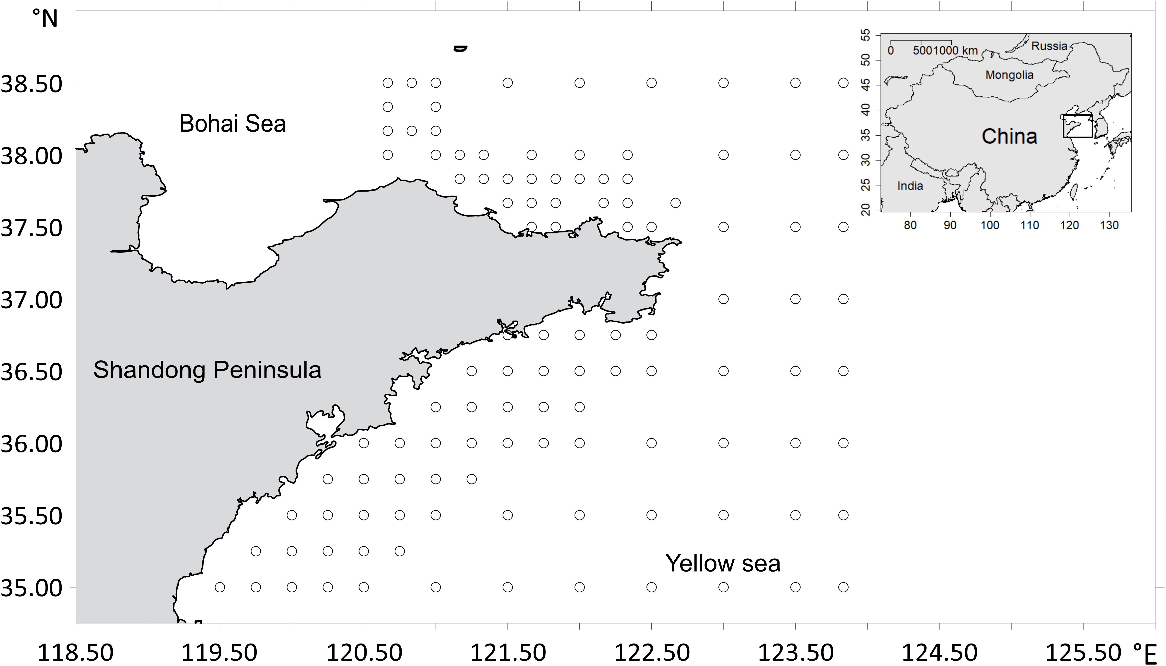
Figure 1. Map of survey stations in the coastal waters of Shandong Peninsula.

TABLE 1

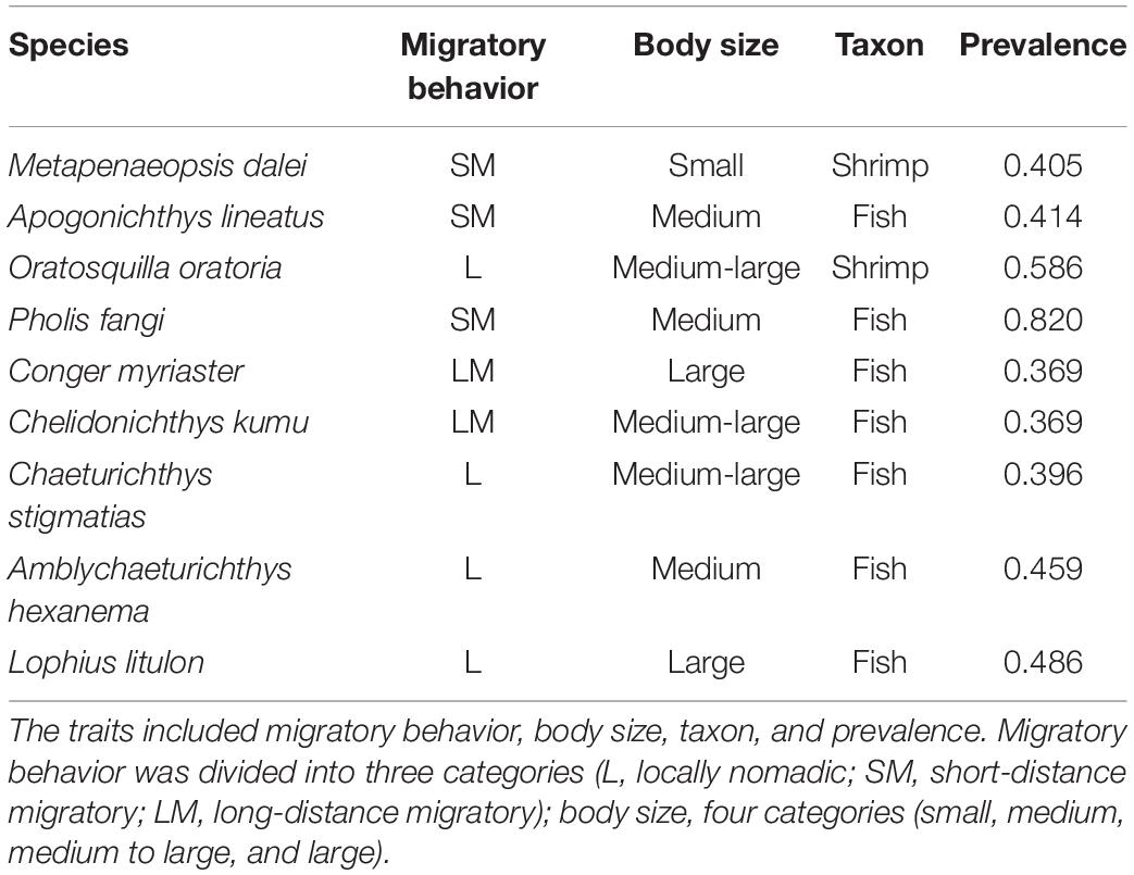
Table 1. Summary of biological traits of the nine demersal species being modeled.

The candidate environment predictors in distribution modeling consisted of sea bottom salinity (BS), sea bottom temperature (BT), water depth (DP), and sediment type (SD). The temperature, salinity, and depth were recorded by the CTD system (XR-420) at the beginning of each tow in each sampled station. The sediment type included three categories, sand, sandy silt, and sand–silt–clay, which follow Shepard’s nomenclature of sediments (Shepard, 1954; data were unpublished and were provided by the College of Environmental Science and Engineering, Ocean University of China). We also considered two geographical coordinates (longitude, LN and latitude, LT) as the explanatory variables, which can serve as surrogates of unobserved environmental factors, given the existence of Yellow Sea cold-water mass. We used the variation inflation factor (VIF) to examine the collinearity between predictive variables before model construction (Parra et al., 2017). The VIF value of a variable that was higher than 3 implied substantial correlations with other variables and was thus omitted.

Here, we assumed three scenarios that presented the availability of the three data types (i.e., response variables) (Table 2). Our trawl surveys in the coastal waters of the Shandong peninsula collected abundance data, and we created occurrence data and ordinal data through the transformations of the abundance in our analyses. It should be noted that the occurrence data and ordinal data may be collected from other sources in practical use, and the transformation is only needed for our evaluation study. Firstly, the ordinal categorical abundance was obtained by binning the abundance data, for which a “k-means cluster” binning strategy in R “arules” package was applied to convert continuous abundance into ordinal categorical abundance with five classes (0, 1, 2, 3, and 4) (Supplementary Appendix Figure 1). The interval boundaries for discretization among nine target species were calculated automatically and listed in Supplementary Appendix Table 1. For the occurrence data, every site that had an abundance category > 0 received a binary occurrence value of “1” (i.e., the presence of species), while the remained sites were coded as “0” (i.e., the absence of species). The generation of P/A and ordinal abundance mimic the situations in which abundance data were not available. In each scenario, the available data type was served as the response variable in the modeling process (Table 2).

TABLE 2

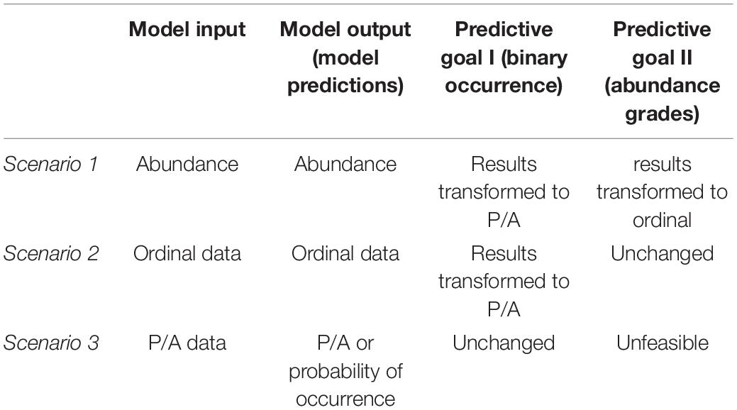
Table 2. The workflow of models built with three types of data (three scenarios) for achieving two predictive goals.

Statistical Modeling Algorithms

As the comparison among data types may be biased due to different modeling algorithms, we utilized two established-well modeling algorithms, GAM and RF, to developed models based on the three data types. The algorithms are described below.

The generalize additive model (GAM) is a semiparametric regression method featured by additive constituents and “smooth” functions (Hastie and Tibshirani, 1990). The merits of GAMs are flexibility in tackling non-linear and non-monotonic relationships. Here, we dealt with different types of response variable through setting the error distribution of GAMs with binomial family for presence/absence data, “ocat” family proposed by Wood et al. (2016) for ordinal categorical data, and gaussian family for log-transformed abundance data. Its formulation is expressed as:

$$g\left(Y\right)=\mathrm{\alpha }+\sum _{i=1}^n{f}_i(x_i)+\mathrm{\epsilon }$$

where, g() is the monotonic link function that establishes a relationship between the mean of the response variable and predictive variables, and f_i is the spline smoothing function of each explanatory variable x_i, which enables to flexibly describe non-linear relationships (Guisan et al., 2002). In the equation α is the intercept, n is the number of explanatory variables, and ε is the residual error term.

Random Forest (RF) (Breiman, 2001) served as a representative of the ML algorithms due to its improving predictive performances (Cutler et al., 2007; Olaya-Marín et al., 2013; Li et al., 2017). RFs were implemented according to the following steps: (i) draw n_tree sets of bootstrap samples and m_try random subset of predictors to product non-pruned regression and classification tree learners (ii) at each node of trees, the predictor was selected for the best binary split and the samples were partitioned recursively until the root node contained a bootstrap sample of data (iii) the predictions from the trees were averaged in the case of regression trees or tallied using a voting system for classification trees (Liaw and Wiener, 2002; Luan et al., 2018). In our study, we applied the randomForest() in the randomForest package in R program. If the response is a factor, randomForest performs classification; if the response is continuous (that is, not a factor), randomForest performs regression. Note that randomForest does not handle ordinal information in the categorical responses (Breiman, 2001). Additionally, the number of trees (n_tree) was set to 2000, and we trained models with different m_try values and chose the optimal m_try = 1 when RF performed best.

For all the models, significant predictors were selected using a stepwise variable selection procedure, in which the model was updated by adding the variables one-by-one, starting with a null model. The applied criterion of variable selection varied from different algorithms and data types. For GAMs, “deviance explained” and AIC among the nested models were used in model selection and to examine the variable importance (Jensen et al., 2005; Li et al., 2017). For RFs, the out-of-bag estimate of error rate was applied for modeling the P/A and ordinal categorical data, whereas the percentage of variance explained by the model (“variance explained”) was used for the abundance data, accordingly (Breiman, 2001). After the stepwise variable selection, all optimal fitted models with different combinations of significant environmental variables using three data types for the nine species were listed in Supplementary Appendix Table 2. Here, the significant environment covariate sets in optimal models may vary depending on the aspect of distribution, i.e., the types of distribution data. Thus, our study aims to select the most simplistic models with the best fitting capacity to further obtain corresponding predictive performance.

Performance Evaluation

The predictive performances of the models (both GAM and RF) based on P/A, and ordinal and abundance data were evaluated under predictive goal I (binary occurrence) and predictive goal II (abundance grades), respectively, followed by the procedure in Table 2. Regarding the capacity of forecasting the binary occurrence (goal I), the models trained by the three data types (three scenarios) were compared, for which the outputs of the ordinal and abundance-based models were transformed into presence/absence according to the same rule as in data transformation (section “Data Collection”) to allow for the direct comparison. Regarding the ability to project the abundance grades (goal II), only models trained by ordinal and abundance data (scenario 1 and 2) were compared, as the abundance grades could not be obtained from occurrence models. The output of abundance-based models was transformed into the categorical abundance to compare predictive accuracies of abundance classifications (Table 2).

The model performance evaluation was implemented using the cross-validation approach, in which 75% of the data were randomly sampled as training data for model fitting, while the remaining 25% were used as testing data to make predictions (i.e., model outputs) and evaluation. This cross-validation process was conducted for 100 replicates, and a number of predictive accuracy measures were estimated by comparing the model predictions with the observations in the testing dataset (Liu et al., 2011).

The accuracy of predicting binary occurrence (predictive goal I) was assessed applying four metrics of discrimination capacity, Cohen’s Kappa (Cohen, 1960), the area under the curve (AUC) of the receiver operating characteristic (Fielding and Bell, 1997), sensitivity (Se), and specificity (Sp), which were widely used in SDM validations (Liu et al., 2011). Among them, Cohen’s Kappa measures the agreement between observations and predictions comparing it with the expected agreement by chance, ranging from −1 to 1 with Kappa value below 0 indicating a prediction no better than random. Kappa values > 0.75 indicate excellent prediction, 0.4–0.75 for good predictions and <0.4 for poor predictions. AUC is a threshold-independent metric, independent of species prevalence (McPherson et al., 2004; Liu et al., 2011). Its values range from 0 to 1, with 0.5 indicating random sorting and 1 indicating perfect prediction (Swets, 1988). Se refers to the probability that a known presence is correctly predicted, and Sp indicates the probability that the model correctly predicts the absence of species.

The accuracy of predicting abundance grades (predictive goal II) was assessed by applying weighted Kappa (Cohen, 1968) regarding the discrimination capacity among abundance grades (Janitza et al., 2016). The weighted Kappa can recognize the levels of classification mistake from models by assigning the weights for the degrees of disagreements between ordinal classes (i.e., the “distances” between the true classification and the predicted one) (Ben-David, 2008).

The differences in the predictive performance among data types, modeling algorithms, and species being modeled were tested by multiway ANOVA, for different performance metrics separately. Here, we selected AUC (for predictive goal I) and weighted Kappa (for predictive goal II) as the dependent variables, and three influencing factors (i.e., data type, algorithm, and species) as the independent variables. We considered that the two performance measures indicate the relatively comprehensive accuracy index in the performance evaluation process. The interaction between data types and algorithms was examined to detect whether the effect of data types might vary among algorithms. We estimated the effects of each factor according to the coefficient in multiple linear regression models of the same structure. All analyses were implemented in R.

Comparisons of Predicted Spatial Distributions

We used the finite volume coastal ocean model (FVCOM) to simulate the hydrological environmental data covering the whole studied area for forecasting the spatial distributions. The FVCOM was developed and its implementation was detailed by the published literature (Xing et al., 2020). In this study, the 42,975 simulated environmental information grid points were extracted from the FVCOM hindcasts in August, 2017. We applied the RF built with the three species data types to generate spatial distribution maps, in which the spatial predictions from distinct response data were transformed into binary distributions (i.e., distribution range) or abundance grades for direct comparison. We examined comparisons of one target species for accurate spatial mapping.

Results

Predictive Performances on Species Occurrences

The predictive performances on species occurrences were compared between models trained with three types of response data applying two modeling algorithms, and the results of O. oratoria were firstly shown as an example (Figure 2). The rank order of data type in predictive accuracy did not vary between AUC and Kappa, but had variances between sensitivity (Se) and specificity (Sp). Specifically, RFs showed that occurrence data achieved relatively great capacity (moderate sensitivity and specificity and overall best discrimination capacity (i.e., the highest values of AUC and Kappa)). On the contrary, abundance data led to the highest sensitivity but the lowest specificity. When using the GAM algorithm, the models trained with ordinal data displayed the best performances, and the results of sensitivity and specificity were consistent with that of RF.

FIGURE 2

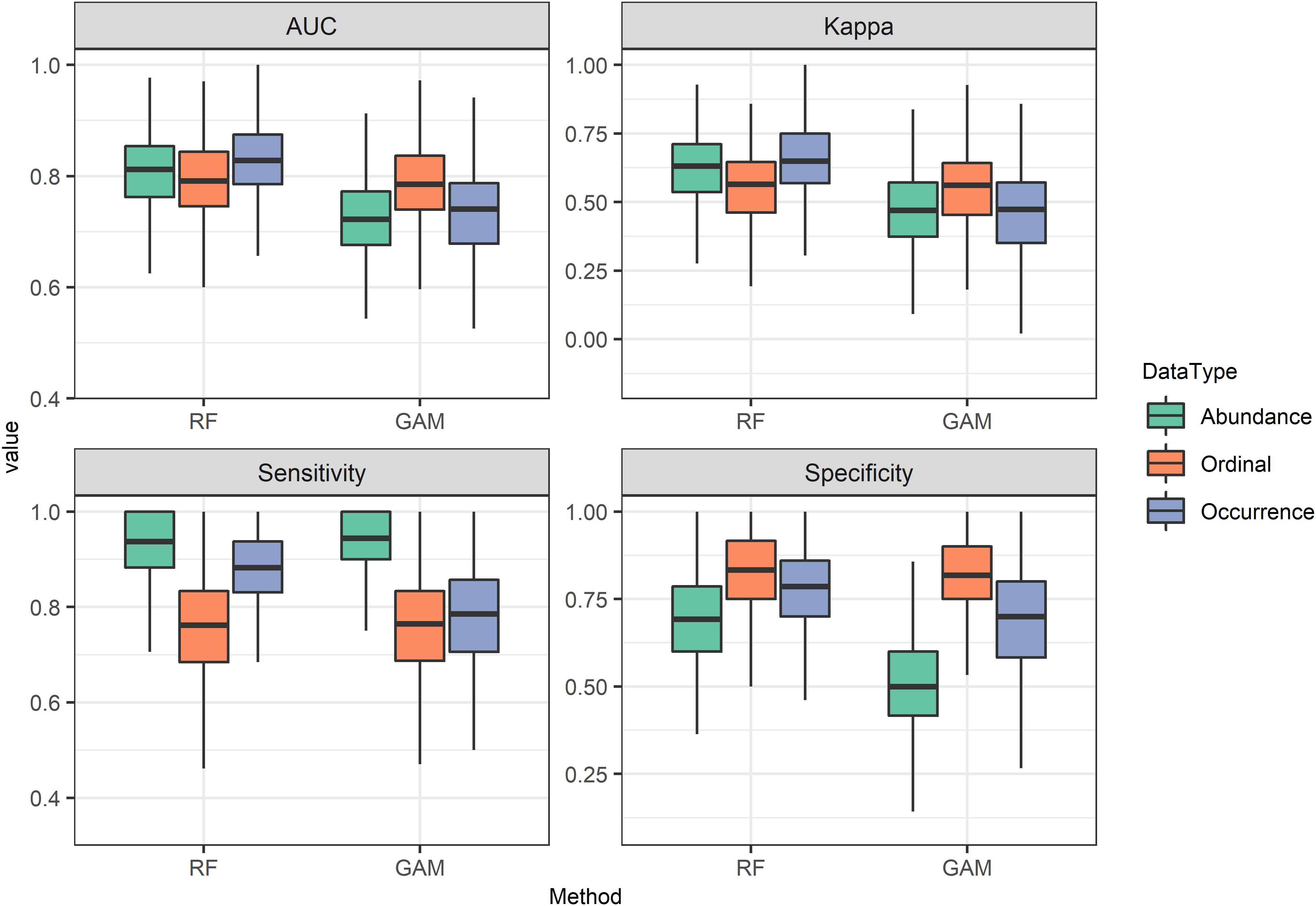
Figure 2. The accuracy metrics for predicting occurrence of O. oratoria between the models based on three data types in two modeling algorithms.

Overall, in terms of AUC, the results of the nine species suggested that occurrence data led to the best predictive performances when RF was used, followed by abundance data, and ordinal data might result in substantially worse performances (Figure 3). On the contrary, when GAM was used for modeling, ordinal data could contribute to the best predictive performances. Meanwhile, there were remarkable divergences between data types among three species, encompassing P. fangi, C. myriaster, C. kumu.

FIGURE 3

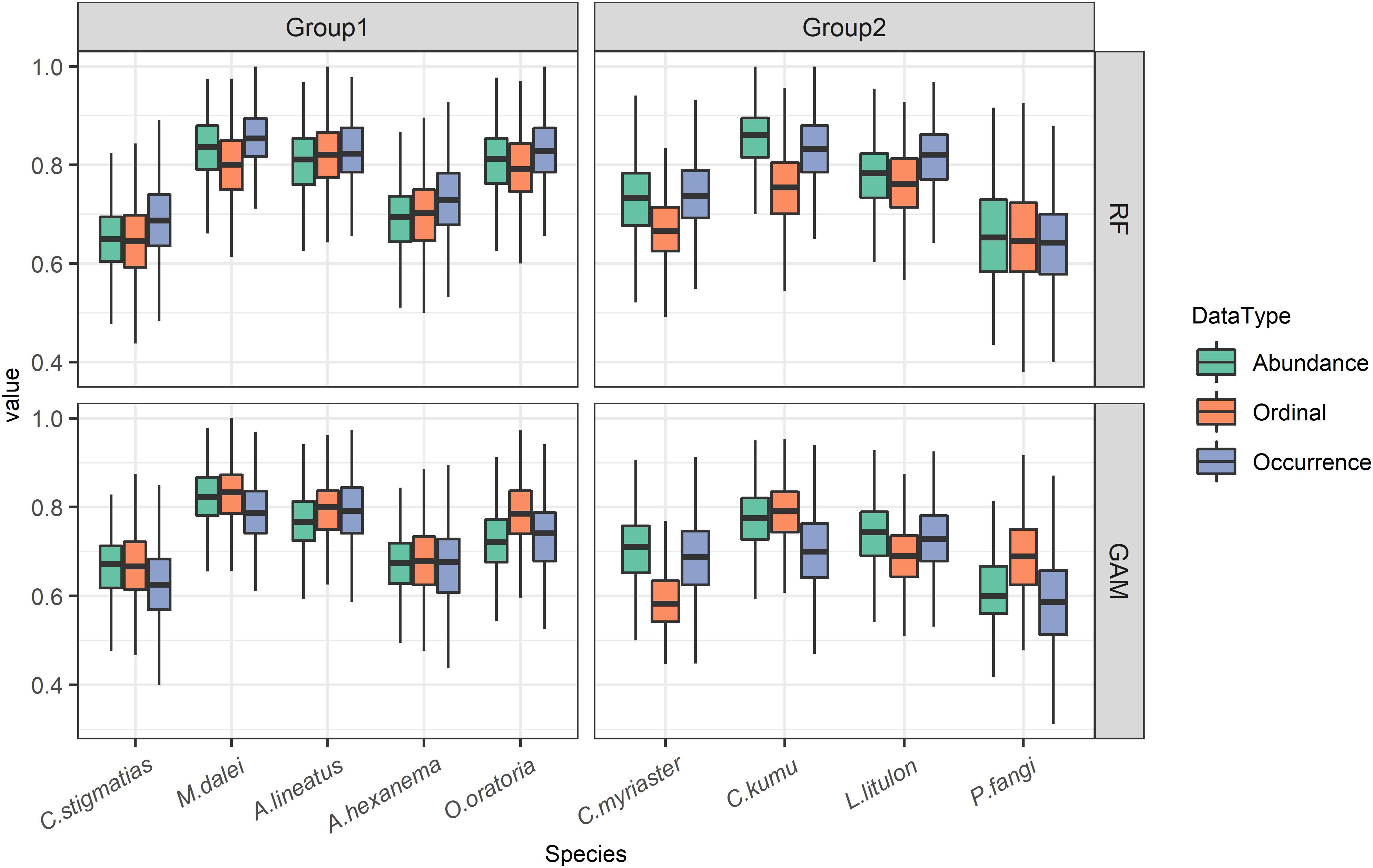
Figure 3. The accuracy metric (AUC) of models trained with three data types for 9 demersal species in terms of predicting occurrence.

The predictive performances were further evaluated among the nine species, which was divided into two groups for better comparison (Figure 3). Species group1 included C. stigmatias, M. dalei, A. lineatus, A. hexanema, and O oratoria, representing small–medium shrimp and fish with limited dispersal ability. This group showed a similar level of model performances in terms of different data types (i.e., three scenarios). On the contrary, species group2 exhibited larger discrepancies in predictive accuracy between data types. This group included C. myriaster, C. kumu, L. litulon, P. fangi, representing medium-large organisms with long-distance migration. Combination of the results from RF and GAM, uses of ordinal data generally contributed to the poorest model performance amongst three data types when modeling species group 2.

Predictive Performances on Abundance Grades

The predictive performances on abundance grades were compared between models utilizing abundance and ordinal data, and the results of L. litulon were shown as an example. Given the challenge of multilevel prediction, both of the models yielded remarkable misclassification. The abundance-based models were more discriminating for the medium-ranked classifications but had substantial error rates in the lowest and highest grades. By contrast, ordinal-based models had a greater capacity to classify the lowest and highest classes, but underestimated the probability of medium-ranked classes. Besides, the prediction of abundance-based models tended to bias to presence whereas ordinal-based models were more likely to predict absence of species occurrence (Figure 4). The resultant comparisons of predicted classifications from other eight species using two data types were analogous to that of L. litulon (see Supplementary Appendix Figure 2).

FIGURE 4

Figure 4. The ordinal categorical predictions of L. litulon from the models using two data types.

The metric of ability to predict abundance grades, weighted Kappa, were compared between uses of ordinal and abundance data across the nine species, which were assigned to the same species groups as section “Predictive Performances on Species Occurrences.” Regarding RFs, the weighted Kappa indicated that abundance data could marginally improve predictions compared to ordinal data (Figure 5). Regarding GAMs, ordinal-trained models performed better in terms of weighted Kappa, except C. myriaster that abundance-trained models predicted more accurately.

FIGURE 5

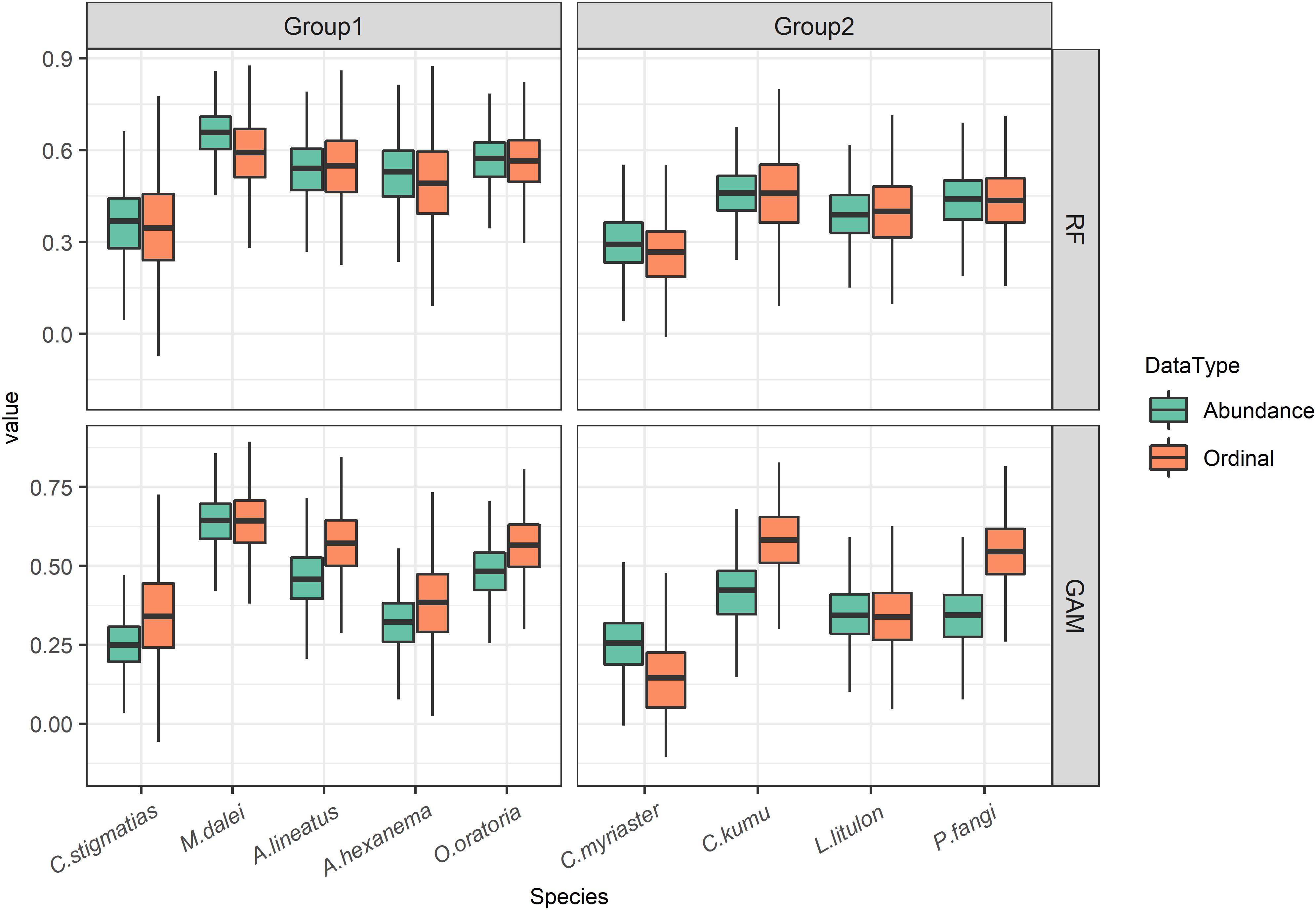
Figure 5. The accuracy metric (weighted Kappa) of models trained with two data types in terms of predicting abundance grades.

In addition, the differences in predictive accuracy between data types were more remarkable when using GAMs compared to that of RFs (Figure 5). For the GAM algorithm, there were discrepancies between uses of two data types in six species cases, expect for M. dalei, A. hexanema, and L. litulon. While most species in the two groups showed less difference between the two data types in the RF algorithm, with the exception of M. dalei, which showed better discrimination capacity using abundance data.

The Effects on Predictive Performance

ANOVA showed that the performance metric AUC varied significantly between algorithm (P < 0.01) and species (P < 0.01), whereas the effect of data types was insignificant (P > 0.05) (Table 3). Specifically, according to the estimates fitted by the multiple linear regression, RF algorithm significantly provided better predictive accuracy than GAM. In terms of species, there was a large difference in AUC among species being modeled, and M. dalei was better predicted than other species, following by A. lineatus.

TABLE 3

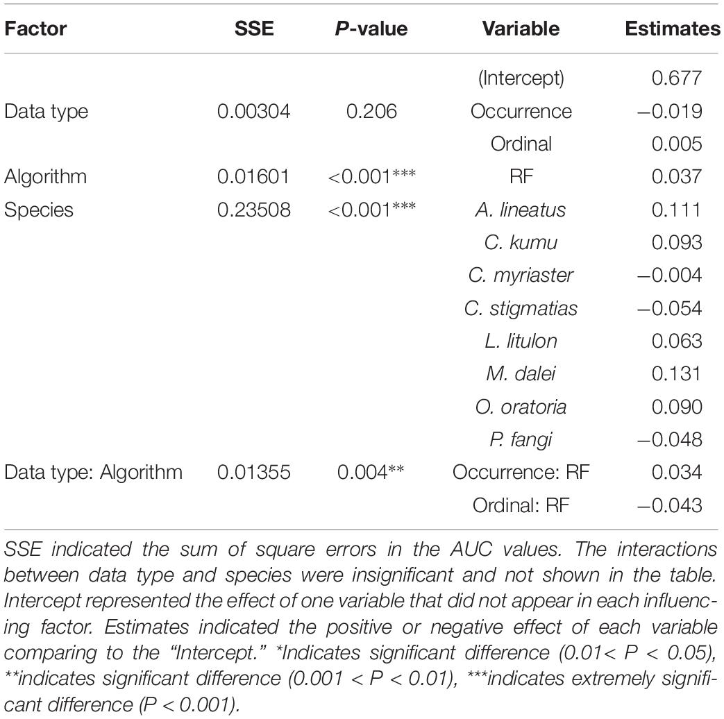
Table 3. The effects of data type, algorithm and species on performance metric (AUC) for predictions on binary occurrence by ANOVA.

The interaction between the effects of data types and algorithms was highly significant (P < 0.01), implying the relative predictive accuracies of each data type varied between RF and GAM (Table 3). When applying the RF algorithm to predict the binary occurrence, P/A data generated better predictions (0.748, estimated coefficient in the regression model) than abundance (0.714), followed by ordinal data (0.671). For the GAM algorithm, models built with ordinal data marginally outperformed (0.682) the counterparts with abundance data (0.677) and occurrence data (0.658).

In terms of weighted Kappa (to predict abundance grades), algorithm and species had a significant influence on predictability (P < 0.01), respectively, Whereas, there were no significant differences among data types (P > 0.05) (Table 4). Regarding species, the model performance was the highest for M. dalei, followed by O. oratoria. Similar to the results of AUC, the interaction between the effects of data type and algorithm was significant for the variance of weighted Kappa (P < 0.05), i.e., for RF, the abundance-based models (0.444) performed better than ordinal-based models (0.375), and the converse was true for GAM (abundance: 0.377, ordinal: 0.442). Combined with the results of the two algorithms, abundance data exhibited slightly better discriminations.

TABLE 4

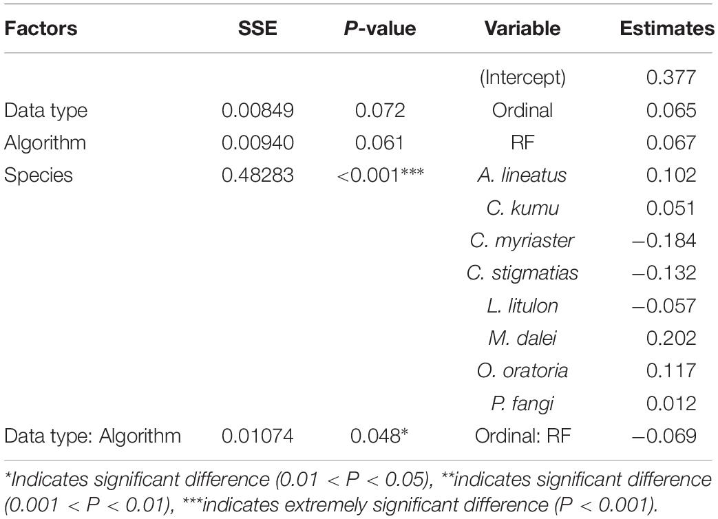
Table 4. The effects of data type, algorithm and species on performance metric (weighted Kappa) for predictions on abundance grades by ANOVA.

Comparisons of Spatial Mapping

The predicted spatial distributions of one target organism (M. dalei) by RFs with distinct response data types were mapped according to the two predictive goals for visual comparisons. For projecting the distribution ranges (predictive goal I) (Figure 6), in the southern waters of the study area, the inaccurate ordinal data showed an inferior capacity to identify the presences than other data (Figure 6B). Besides, models built with abundance and ordinal data overestimated the range size of M. dalei in the northern waters. For predicting the abundance grades (predictive goal II) (Figure 7), the discrepancy in spatial predictions between the two data types was greatly obvious, especially in the southern nearshore and the northern waters. The ordinal-based model tended to simulate higher abundance for M. dalei and showed worse predicted classifications in the northern area (Figure 7B).

FIGURE 6

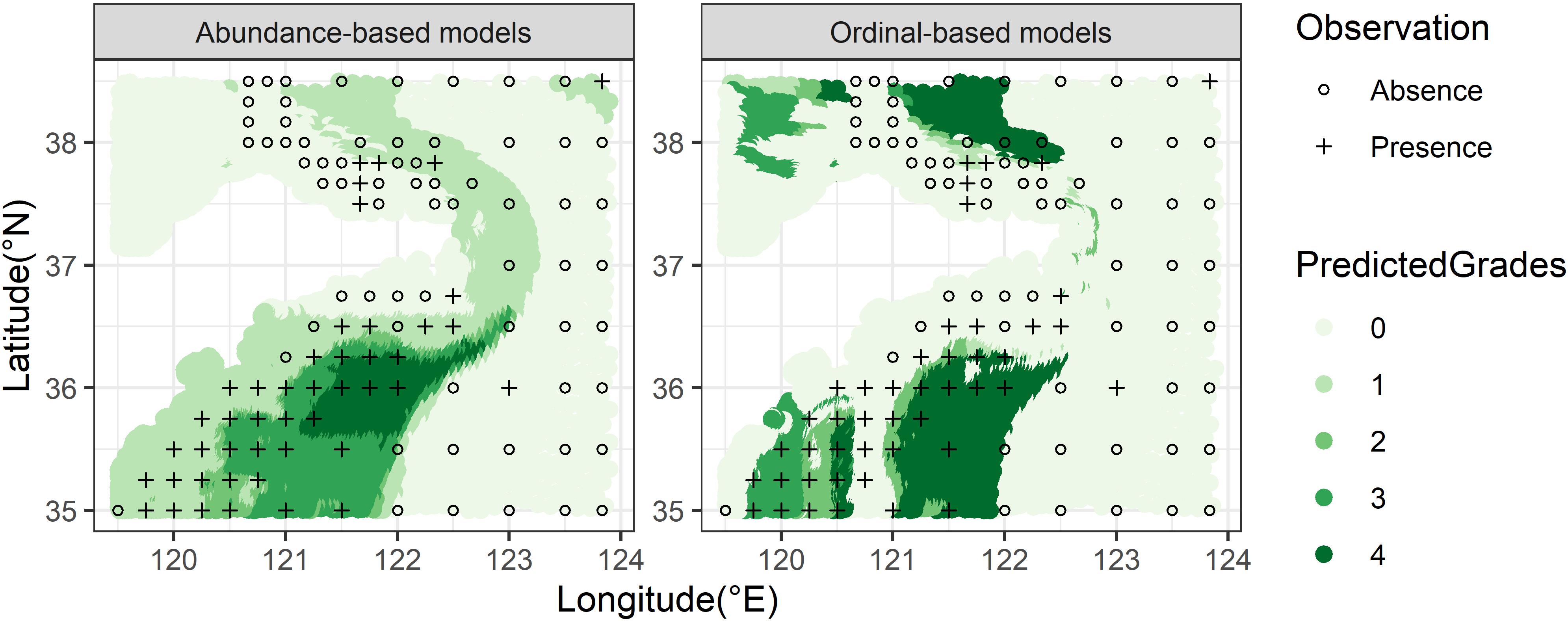
Figure 6. The predicted (color circles) distribution ranges of M. dalei by RF for uses of three species data types in the coastal waters of Shandong Peninsula. The overlying hollow circles indicates the observed stations with absence, and the overlying cross indicates observed stations with presence.

FIGURE 7

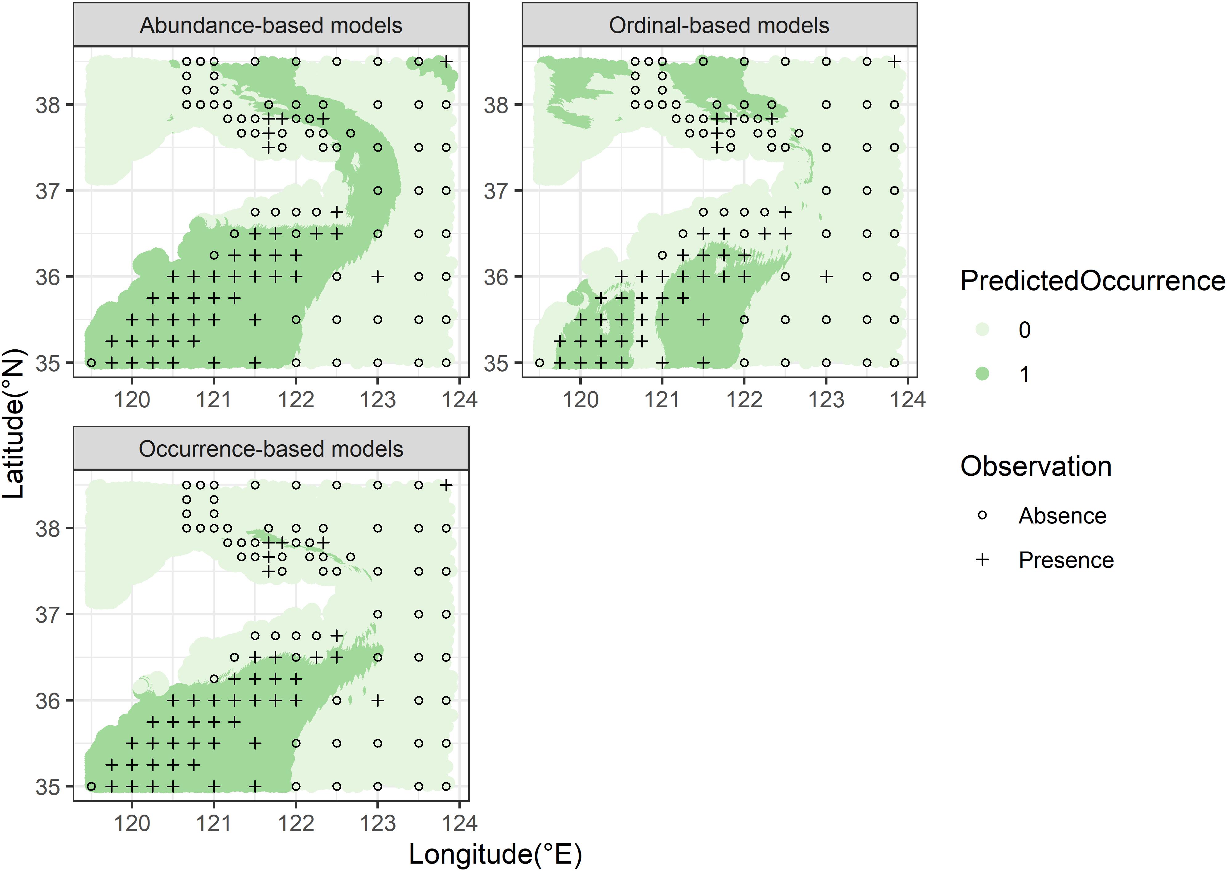
Figure 7. The predicted (color circles) abundance grades of M. dalei by RF for uses of two species data types in the coastal waters of Shandong Peninsula.

Discussion

Increasing uncertainty in the predictability of SDMs and extensive applications toward forecast impelled researchers to enhance the understanding of model assessment. Selection of response dataset types essentially makes a difference in model performances, and unquestionably, higher data quality contributes to greater model projections. However, the limited availability of accurate observations has quickened a growing utilization of georeferenced distribution data for model simulations. Most notably, some applications only required provisions of rough abundance grades or distribution ranges and boundaries. Thus, the model capacity we concerned was not to quantitatively predict accurate abundance, but to qualitatively describe the distribution patterns of an organism. In this context, we assumed three scenarios based on the availability of the three data types to clarify whether less informative data types could be reliable for qualitative predictions without implements of the sampling survey. In general, our results illustrated that the effect of data type on predictability was varied across modeling methods, species and two predictive application goals, and even in some cases, P/A data were more reliable for providing occurrence projections as well as ordinal data were marginally better (but insignificantly) for distinguishing abundance grades since abundance data failed to perform better. Whereas, combined with two algorithms, ANOVA showed that the abundance data was slightly better than the ordinal data. Why abundance data might not necessarily bring outperformances? Preliminarily, due to the complexity and dynamics of the marine environment (Oppel et al., 2012), abundance observations in fisheries surveys tend to contain higher uncertainty originating from observation error, imperfect detectability and improper sample designs (Pearce and Ferrier, 2001; Briscoe et al., 2019), which may undermine the processes of model fitting and offset the advantage of rich information. Apart from the possibility of sampling deficiency, the convincing biological explanation is that environmental factors that are influential for species occurrence may not be the same for species abundance, for instance, a higher suitability of habitat at a location might not be correlated with a larger number of individuals and long persistence time for species presence (Acevedo et al., 2017). The argument behind this explanation is that the relationship between habitat suitability and abundance has been widely debated (Pearce and Ferrier, 2001). In this study, the higher specificity index revealed that uses of ordinal data were prone to predict the absence of a species, which was supported by the viewpoint from VanDerWal et al. (2009) that habitat suitability could indicate the upper limit of abundance and abundance is low with decreased habitat suitability. Whereas, using abundance data showed converse consequence, which might attribute to the methodological aspect that abundance-based models hardly predicted a zero abundance. Moreover, distribution models could more easily capture the responses of species occurrence to the environment at larger spatial scales and coarse resolutions than the responses of abundance (Pearce and Ferrier, 2001; Fukuda et al., 2012).

Implications

The fact that the effects of data types on model performances may be case specific implies that proper response data with the cost-effective collection process may be considered for achieving specific habitat research objectives. Specifically, when binary occurrence details serve as the predictive target to satisfy the applications, such as identifying habitat preferences (Thuiller, 2004) and planning for spatial conservation (Guisan et al., 2013) (i.e., requirement for prediction precision are relatively low), the P/A data can be recommended as the reliable input of SDMs when abundance is unavailable. Meanwhile, when grades of abundance serve as the target to inform the applications, such as delineation of habitat quality, assessment of MPA effects, and forecasting the center of gravity of species distributions (Pearce and Ferrier, 2001; Fukuda et al., 2012; Thorson et al., 2017), using the relatively coarse abundance categories combined with designated modeling techniques (like GAM) may be an alternative to the application of accurate abundance data, if survey funding and time are limited.

Furthermore, the effects of data types on model predictive performance vary among demersal species, probably implying that their intrinsic traits have an impact on the influence of data types on predictive performances. Particularly, for the targets of predictions on occurrences, the shrimps and non-resident fish with moderate prevalence (i.e., species group1) showed fewer discrepancies in predictability among data types, suggesting that the effort to obtain response data for these species could be largely mitigated. Furthermore, our finding agreed with the idea from recent literature, that the predictive accuracies of P/A-based models were more sensitive to species prevalence than abundance-based models (Fukuda et al., 2012; Howard et al., 2014) and presented marginally inferior performance when modeling species with relative low/high prevalence (Figure 3).

The ANOVA analysis revealed that the effects of data types on predictive accuracy might substantially depend on distinct algorithms applied, which might associate with the distinct data processing behaviors (Marmion et al., 2009). With the implementation of GAM, the better performance with the ordinal data might benefit from applying an appropriate error distribution assumption (i.e., “ocat” family). Regarding the RF algorithm, the classical RF by randomForest package is incapable of recognizing the ordinal nature of data, (i.e., treats the ordinal variable as nominal). Notably, RF showed consistent resultant rankings of data types among all modeled species compared to GAM, possibly resulting from its “bagging” and “ensemble” ideas for creating many sampling sets that could produce stable predictions (Breiman, 2001).

Limitations and Perspectives

Although our assessment framework was implemented reasonably from a practical viewpoint, there existed some limitations. First, our analysis compared the model performances based on different data types but of the same sample size. However, an important fact is that with the same survey cost and sampling intensity spent or the same effort applied in obtaining information from georeferenced data sources, more recorded points of occurrence data can be collected than that of abundance data. This implies that our comparisons provide only a baseline and the models based on information-poor data may perform better in practice than that in our simulations. Besides, it is also acknowledged that the SDMs simulated species potential distributions based on the concept of the fundamental niche (Hutchinson, 1957) without consideration of abiotic factors and interspecific relationships (Kearney and Porter, 2009). Thus, there was no guarantee that the same comparing results can be brought out if the realized niche was required to be projected. Being unable to cover the geographical extent and ranges of migratory and generalist species might bring out little understanding of their environmental adaptions in the habitat patches, influencing models to correctly determine the species responses to habitat. As a consequence, some conclusions may require further validation before being applied in different marine ecosystems and spatial scales.

As the traditional correlative SDMs in our study might fail to take full advantage of the information details in abundance data, we recommend that the application of spatial abundance information to dynamic SDMs or dynamic range models by including explicit demographical processes, such as population dynamics and dispersal in distribution modeling (Keith et al., 2008; Mieszkowska et al., 2013; Briscoe et al., 2019), thus allowing for a time series of future abundance and expected persistence times of local populations. We can foresee that with the emergence of novel algorithms, further model simulations, and assessment for other types of response data could supply additional approaches to settlement ecological questions.

Conclusion

Ecologists have always been eager for better datasets, especially long-term temporal data of species abundance covering an appropriate spatial scale and frequency (Joseph et al., 2006), as quantitative data are essentially richer in information than qualitative data. Additionally, as an increasing number of global databases are available to provide periodic atlases, more detailed data may be more important in the future. Nevertheless, our designed evaluation process put the results into new perspectives on the selection of datasets. Significantly, this study demonstrated that no data type was superior in any situation, and the effect of data types substantially varied by the algorithms implemented. The mixed results possibly related to the complex dynamics of marine ecosystems and influencing factors on occurrence–abundance relationship (Nielsen et al., 2005; Gutiérrez et al., 2013), suggesting that matching data types for the predictive targets of the SDMs should be based on specific circumstances, depending on algorithms, and species groups of diverse ecological traits. Our implications would possibly alleviate the pressures from suspicion of the reliability of rough distribution data to an extent. We also underlined the importance of richer data content in model constructions and simulations, despite a slight advantage in applying abundance data.

Data Availability Statement

The original contributions presented in the study are included in the article/Supplementary Material, further inquiries can be directed to the corresponding author/s.

Ethics Statement

The animal study was reviewed and approved by College of fisheries, Ocean University of China.

Author Contributions

JL: data curation, methodology, writing-original draft, writing-review and editing, and software. CZ: conceptualization, writing-review and editing, and supervision. YJ and YX: validation and supervision. BX: conceptualization and investigation. YR: funding acquisition and supervision. All authors contributed to the article and approved the submitted version.

Funding

This work was supported by the National Key R&D Program of China (2018YFD0900904 and 2018YFD0900906).

Conflict of Interest

The authors declare that the research was conducted in the absence of any commercial or financial relationships that could be construed as a potential conflict of interest.

Publisher’s Note

All claims expressed in this article are solely those of the authors and do not necessarily represent those of their affiliated organizations, or those of the publisher, the editors and the reviewers. Any product that may be evaluated in this article, or claim that may be made by its manufacturer, is not guaranteed or endorsed by the publisher.

Acknowledgments

The authors thank the editor and the two reviewers for their review and comments on the manuscript. The authors would like to thank the colleagues of the Fishery Ecosystem Monitoring and Assessment (FEMA) Laboratory of Ocean University of China for their help in sample collection and experimental assistance. The authors would also like to thank Yunzhou Li for her help in improving the language of this manuscript.

Supplementary Material

The Supplementary Material for this article can be found online at: https://www.frontiersin.org/articles/10.3389/fmars.2021.771071/full#supplementary-material

References

Acevedo, P., Ferreres, J., Escudero, M. A., Jimenez, J., Boadella, M., and Marco, J. (2017). Population dynamics affect the capacity of species distribution models to predict species abundance on a local scale. Divers. Distrib. 23, 1008–1017. doi: 10.1111/ddi.12589

CrossRef Full Text | Google Scholar

Austin, M. P., and Van Niel, K. P. (2011). Improving species distribution models for climate change studies: variable selection and scale. J. Biogeogr. 38, 1–8. doi: 10.1111/j.1365-2699.2010.02416.x

CrossRef Full Text | Google Scholar

Beck, J. L., Dauwalter, D. C., Gerow, K. G., and Hayward, G. D. (2010). Design to monitor trend in abundance and presence of American beaver (Castor canadensis) at the national forest scale. Environ. Monit. Assess. 164, 463–479. doi: 10.1007/s10661-009-0907-8

PubMed Abstract | CrossRef Full Text | Google Scholar

Bellard, C., Bertelsmeier, C., Leadley, P., Thuiller, W., and Courchamp, F. (2012). Impacts of climate change on the future of biodiversity. Ecol. Lett. 15, 365–377. doi: 10.1111/j.1461-0248.2011.01736.x

PubMed Abstract | CrossRef Full Text | Google Scholar

Ben-David, A. (2008). Comparison of classification accuracy using Cohen’s Weighted Kappa. Expert Syst. Applic. 34, 825–832. doi: 10.1016/j.eswa.2006.10.022

CrossRef Full Text | Google Scholar

Breiman, L. (2001). Random forests. Mach. Learn. 45, 5–32. doi: 10.1023/A:1010933404324

CrossRef Full Text | Google Scholar

Briscoe, N. J., Elith, J., Salguero-Gómez, R., Lahoz-Monfort, J. J., Camac, J. S., Giljohann, K. M., et al. (2019). Forecasting species range dynamics with process-explicit models: matching methods to applications. Ecol. Lett. 22, 1940–1956. doi: 10.1111/ele.13348

PubMed Abstract | CrossRef Full Text | Google Scholar

Brosse, S., Guegan, J. F., Tourenq, J. N., and Lek, S. (1999). The use of artificial neural networks to assess fish abundance and spatial occupancy in the littoral zone of a mesotrophic lake. Ecol. Model. 120, 299–311. doi: 10.1016/S0304-3800(99)00110-6

CrossRef Full Text | Google Scholar

Brotons, L., Thuiller, W., Araujo, M. B., and Hirzel, A. H. (2004). Presence-absence versus presence-only modeling methods for predicting bird habitat suitability. Ecography 27, 437–448. doi: 10.1111/j.0906-7590.2004.03764.x

CrossRef Full Text | Google Scholar

Cohen, J. (1960). A coefficient of agreement for nominal scales. Educ. Psychol. Meas. 20, 37–46. doi: 10.1177/001316446002000104

CrossRef Full Text | Google Scholar

Cohen, J. (1968). Weighted kappa: nominal scale agreement provision for scaled disagreement or partial credit. Psychol. Bull. 70:213. doi: 10.1037/h0026256

PubMed Abstract | CrossRef Full Text | Google Scholar

Cutler, D. R., Edwards, T. C. Jr., Beard, K. H., Cutler, A., Hess, K. T., Gibson, J., et al. (2007). Random forests for classfication in ecology. Ecology 88, 2783–2792. doi: 10.1890/07-0539.1

CrossRef Full Text | Google Scholar

de Araújo, C. B., Marcondes-Machado, L. O., and Costa, G. C. (2014). The importance of biotic interactions in species distribution models: a test of the Eltonian noise hypothesis using parrots. J. Biogeogr. 41, 513–523. doi: 10.1111/jbi.12234

CrossRef Full Text | Google Scholar

Elith, J., Graham, C. H., Anderson, R. P., Dudík, M., Ferrier, S., Guisan, A., et al. (2006). Novel methods improve prediction of species’ distributions from occurrence data. Ecography 29, 129–151. doi: 10.1111/j.2006.0906-7590.04596.x

CrossRef Full Text | Google Scholar

Elith, J., and Leathwick, J. R. (2009). Species distribution models: ecological explanation and prediction across space and time. Annu. Rev. Ecol. Evol. Syst. 40, 677–697. doi: 10.1146/annurev.ecolsys.110308.120159

CrossRef Full Text | Google Scholar

Fernandes, R. F., Scherrer, D., and Guisan, A. (2019). Effects of simulated observation errors on the performance of species distribution models. Divers. Distrib. 25, 400–413. doi: 10.1111/ddi.12868

CrossRef Full Text | Google Scholar

Fielding, A. H., and Bell, J. F. (1997). A review of methods for the assessment of prediction errors in conservation presence/absence models. Environ. Conserv. 24, 38–49. doi: 10.1017/S0376892997000088

CrossRef Full Text | Google Scholar

Fukuda, S., Mouton, A. M., and De Baets, B. (2012). Abundance versus presence/absence data for modeling fish habitat preference with a genetic Takagi–Sugeno fuzzy system. Environ. Monit. Assess. 184, 6159–6171. doi: 10.1007/s10661-011-2410-2

PubMed Abstract | CrossRef Full Text | Google Scholar

Gobeyn, S., Mouton, A. M., Cord, A. F., Kaim, A., Volk, M., and Goethals, P. L. (2019). Evolutionary algorithms for species distribution modeling: a review in the context of machine learning. Ecol. Model. 392, 179–195. doi: 10.1016/j.ecolmodel.2018.11.013

CrossRef Full Text | Google Scholar

Guillera-Arroita, G., Lahoz-Monfort, J. J., Elith, J., Gordon, A., Kujala, H., Lentini, P. E., et al. (2015). Is my species distribution model fit for purpose? Matching data and models to applications. Global Ecol. Biogeogr. 24, 276–292. doi: 10.1111/geb.12268

CrossRef Full Text | Google Scholar

Guisan, A., Edwards, T. C. Jr., and Hastie, T. (2002). Generalized linear and generalized additive models in studies of species distributions: setting the scene. Ecol. Model. 157, 89–100. doi: 10.1016/S0304-3800(02)00204-1

CrossRef Full Text | Google Scholar

Guisan, A., Tingley, R., Baumgartner, J. B., Naujokaitis-Lewis, I., Sutcliffe, P. R., Tulloch, A. I, et al. (2013). Predicting species distributions for conservation decisions. Ecol. Lett. 16, 1424–1435. doi: 10.1111/ele.12189

PubMed Abstract | CrossRef Full Text | Google Scholar

Guisan, A., and Zimmermann, N. E. (2000). Predictive habitat distribution models in ecology. Ecol. Model. 135, 147–186. doi: 10.1016/S0304-3800(00)00354-9

CrossRef Full Text | Google Scholar

Guisan, A., Zimmermann, N. E., Elith, J., Graham, C. H., Phillips, S., and Peterson, A. T. (2007). What matters for predicting the occurrences of trees: techniques, data, or species’characteristics? Ecol. Monogr. 77, 615–630. doi: 10.1890/061060.1

CrossRef Full Text | Google Scholar

Gutiérrez, D., Harcourt, J., Díez, S. B., Illán, J. G., and Wilson, R. J. (2013). Models of presence–absence estimate abundance as well as (or even better than) models of abundance: the case of the butterfly Parnassius apollo. Landsc. Ecol. 28, 401–413. doi: 10.1007/s10980-013-9847-3

CrossRef Full Text | Google Scholar

Hastie, T. J., and Tibshirani, R. J. (1990). Generalized Additive Models (Vol. 43). Boca Raton, FL: CRC Press.

Google Scholar

Howard, C., Stephens, P. A., Pearce-Higgins, J. W., Gregory, R. D., and Willis, S. G. (2014). Improving species distribution models: the value of data on abundance. Methods Ecol. Evol. 5, 506–513. doi: 10.1111/2041-210X.12184

CrossRef Full Text | Google Scholar

Hutchinson, G. E. (1957). Concluding remarks. Cold Spring Harbor Symp. Quant. Biol. 22, 145–159. doi: 10.1101/SQB.1957.022.01.039

CrossRef Full Text | Google Scholar

Janitza, S., Tutz, G., and Boulesteix, A. L. (2016). Random forest for ordinal responses: prediction and variable selection. Comput. Stat. Data Anal. 96, 57–73. doi: 10.1016/j.csda.2015.10.005

CrossRef Full Text | Google Scholar

Jensen, O. P., Seppelt, R., Miller, T. J., and Bauer, L. J. (2005). Winter distribution of blue crab Callinectes sapidus in Chesapeake Bay: application and cross-validation of a two-stage generalized additive model. Mar. Ecol. Prog. Ser. 299, 239–255. doi: 10.3354/meps299239

CrossRef Full Text | Google Scholar

Joseph, L. N., Field, S. A., Wilcox, C., and Possingham, H. P. (2006). Presence-absence versus abundance data for monitoring threatened species. Conserv. Biol. 20, 1679–1687. doi: 10.1111/j.1523-1739.2006.00529.x

PubMed Abstract | CrossRef Full Text | Google Scholar

Kearney, M., and Porter, W. (2009). Mechanistic niche modeling: combining physiological and spatial data to predict species’ ranges. Ecol. Lett. 12, 334–350. doi: 10.1111/j.1461-0248.2008.01277.x

PubMed Abstract | CrossRef Full Text | Google Scholar

Keith, D. A., Akçakaya, H. R., Thuiller, W., Midgley, G. F., Pearson, R. G., Phillips, S. J., et al. (2008). Predicting extinction risks under climate change: coupling stochastic population models with dynamic bioclimatic habitat models. Biol. Lett. 4, 560–563. doi: 10.1098/rsbl.2008.0049

PubMed Abstract | CrossRef Full Text | Google Scholar

Li, M., Zhang, C., Xu, B., Xue, Y., and Ren, Y. (2017). Evaluating the approaches of habitat suitability modeling for whitespotted conger (conger myriaster). Fish. Res. 195, 230–237.

Google Scholar

Liaw, A., and Wiener, M. (2002). Classification and regression by randomForest. R News 2, 18–22.

Google Scholar

Liu, C., White, M., and Newell, G. (2011). Measuring and comparing the accuracy of species distribution models with presence–absence data. Ecography 34, 232–243. doi: 10.1111/j.1600-0587.2010.06354.x

CrossRef Full Text | Google Scholar

Luan, J., Zhang, C., Xu, B., Xue, Y., and Ren, Y. (2018). Modeling the spatial distribution of three Portunidae crabs in Haizhou Bay, China. PLoS One 13:e0207457.

Google Scholar

Luan, J., Zhang, C., Xu, B., Xue, Y., and Ren, Y. (2020). The predictive performances of random forest models with limited sample size and different species traits. Fish. Res. 227:105534. doi: 10.1016/j.fishres.2020.105534

CrossRef Full Text | Google Scholar

Marmion, M., Parviainen, M., Luoto, M., Heikkinen, R. K., and Thuiller, W. (2009). Evaluation of consensus methods in predictive species distribution modeling. Divers. Distrib. 15, 59–69. doi: 10.1111/j.1472-4642.2008.00491.x

CrossRef Full Text | Google Scholar

Mateo, R. G., Croat, T. B., Felicísimo, ÁM., and Munoz, J. (2010). Profile or group discriminative techniques? Generating reliable species distribution models using pseudo-absences and target-group absences from natural history collections. Divers. Distrib. 16, 84–94. doi: 10.1111/j.1472-4642.2009.00617.x

CrossRef Full Text | Google Scholar

McPherson, J. M., and Jetz, W. (2007). Effects of species’ ecology on the accuracy of distribution models. Ecography 30, 135–151.

Google Scholar

McPherson, J. M., Jetz, W., and Rogers, D. J. (2004). The effects of species’ range sizes on the accuracy of distribution models: ecological phenomenon or statistical artefact? J. Appl. Ecol. 41, 811–823. doi: 10.1111/j.0021-8901.2004.00943.x

CrossRef Full Text | Google Scholar

Mieszkowska, N., Milligan, G., Burrows, M. T., Freckleton, R., and Spencer, M. (2013). Dynamic species distribution models from categorical survey data. J. Anim. Ecol. 82, 1215–1226. doi: 10.1111/1365-2656.12100

PubMed Abstract | CrossRef Full Text | Google Scholar

Nielsen, S. E., Johnson, C. J., Heard, D. C., and Boyce, M. S. (2005). Can models of presence-absence be used to scale abundance? Two case studies considering extremes in life history. Ecography 28, 197–208. doi: 10.1111/j.0906-7590.2005.04002.x

CrossRef Full Text | Google Scholar

Olaya-Marín, E. J., Martínez-Capel, F., and Vezza, P. (2013). A comparison of artificial neural networks and random forests to predict native fish species richness in Mediterranean rivers. Knowl. Manag. Aquat. Ecosyst. 409, 7–25.

Google Scholar

Olden, J. D., and Jackson, D. A. (2002). A comparison of statistical approaches for modeling fish species distributions. Freshw. Biol. 47, 1976–1995. doi: 10.1046/j.1365-2427.2002.00945.x

CrossRef Full Text | Google Scholar

Oppel, S., Meirinho, A., Ramírez, I., Gardner, B., O’Connell, A. F., Miller, P. I., et al. (2012). Comparison of five modeling techniques to predict the spatial distribution and abundance of seabirds. Biol. Conserv. 156, 94–104. doi: 10.1016/j.biocon.2011.11.013

CrossRef Full Text | Google Scholar

Osborne, P. E., and Leitão, P. J. (2009). Effects of species and habitat positional errors on the performance and interpretation of species distribution models. Divers. Distrib. 15, 671–681. doi: 10.1111/j.1472-4642.2009.00572.x

CrossRef Full Text | Google Scholar

Parra, H. E., Pham, C. K., Menezes, G. M., Rosa, A., Tempera, F., and Morato, T. (2017). Predictive modeling of deep-sea fish distribution in the Azores. Deep Sea Res. Part II Top. Stud. Oceanogr. 145, 49–60. doi: 10.1016/j.dsr2.2016.01.004

CrossRef Full Text | Google Scholar

Pearce, J., and Ferrier, S. (2001). The practical value of modeling relative abundance of species for regional conservation planning: a case study. Biol. Conserv. 98, 33–43. doi: 10.1016/S0006-3207(00)00139-7

CrossRef Full Text | Google Scholar

Pereira, H. M., Leadley, P. W., Proença, V., Alkemade, R., Scharlemann, J. P., Fernandez-Manjarrés, J. F., et al. (2010). Scenarios for global biodiversity in the 21st century. Science 330, 1496–1501. doi: 10.1126/science.1196624

PubMed Abstract | CrossRef Full Text | Google Scholar

Shepard, F. P. (1954). Nomenclature based on sand-silt-clay ratios. J. Sediment. Res. 24, 151–158. doi: 10.1306/D4269774-2B26-11D7-8648000102C1865D

CrossRef Full Text | Google Scholar

Sui, H. Z., Xue, Y., Ren, Y. P., Zhou, Y. Y., and Yu, L. (2017). Studies on the ecological groups of fish communities in Haizhou Bay. China. J. Ocean U. China (Chin. Ed.) 47, 59–71.

Google Scholar

Sundblad, G., Bergström, U., and Sandström, A. (2011). Ecological coherence of marine protected area networks: a spatial assessment using species distribution models. J. Appl. Ecol. 48, 112–120. doi: 10.1111/j.1365-2664.2010.01892.x

CrossRef Full Text | Google Scholar

Swets, J. A. (1988). Measuring the accuracy of diagnostic systems. Science 240, 1285–1293. doi: 10.1126/science.3287615

PubMed Abstract | CrossRef Full Text | Google Scholar

Thorson, J. T., Ianelli, J. N., and Kotwicki, S. (2017). The relative influence of temperature and size-structure on fish distribution shifts: a case-study on Walleye pollock in the Bering Sea. Fish Fish. 18, 1073–1084. doi: 10.1111/faf.12225

CrossRef Full Text | Google Scholar

Thuiller, W. (2004). Patterns and uncertainties of species’ range shifts under climate change. Global Change Biol. 10, 2020–2027. doi: 10.1111/j.1365-2486.2004.00859.x

CrossRef Full Text | Google Scholar

VanDerWal, J., Shoo, L. P., Johnson, C. N., and Williams, S. E. (2009). Abundance and the environmental niche: environmental suitability estimated from niche models predicts the upper limit of local abundance. Am. Natur. 174, 282–291. doi: 10.1086/600087

PubMed Abstract | CrossRef Full Text | Google Scholar

Wood, S. N., Pya, N., and Säfken, B. (2016). Smoothing parameter and model selection for general smooth models. J. Am. Stat. Assoc. 111, 1548–1575. doi: 10.1080/01621459.2016.1180986

CrossRef Full Text | Google Scholar

Xing, Q., Yu, H., Yu, H., Sun, P., Liu, Y., Ye, Z., et al. (2020). A comprehensive model-based index for identification of larval retention areas: a case study for Japanese anchovy Engraulis japonicus in the Yellow Sea. Ecol. Indic. 116:106479. doi: 10.1016/j.ecolind.2020.106479

CrossRef Full Text | Google Scholar

Xue, Y., Guan, L., Tanaka, K., Li, Z., Chen, Y., and Ren, Y. (2017). Evaluating effects of rescaling and weighting data on habitat suitability modeling. Fish. Res. 188, 84–94. doi: 10.1016/j.fishres.2016.12.001

CrossRef Full Text | Google Scholar

Zhang, Z., Xu, S., Capinha, C., Weterings, R., and Gao, T. (2019). Using species distribution model to predict the impact of climate change on the potential distribution of Japanese whiting Sillago japonica. Ecol. Indic. 104, 333–340. doi: 10.1016/j.ecolind.2019.05.023

CrossRef Full Text | Google Scholar