Hurricane Flood Hazard Assessment for the Archipelago of San Andres, Providencia and Santa Catalina, Colombia

Despite the low occurrence of tropical cyclones at the archipelago of San Andres, Providencia, and Santa Catalina (Colombia), Hurricane Iota in 2020 made evident the area vulnerability to tropical cyclones as major hazards by obliterating 56.4 % of housing, partially destroying the remaining houses in Providencia. We investigated the hurricane storm surge inundation in the archipelago by forcing hydrodynamic models with synthetic tropical cyclones and hypothetical hurricanes. The storm surge from synthetic events allowed identifying the strongest surges using the probability distribution, enabling the generation of hurricane storm surge flood maps for 100 and 500 year return periods. This analysis suggested that the east of San Andres and Providencia are the more likely areas to be flooded from hurricanes storm surges. The hypothetical events were used to force the hydrodynamic model to create worst-case flood scenario maps, useful for contingency and development planning. Additionally, Hurricane Iota flood levels were calculated using 2D and 1D models. The 2D model included storm surge (SS), SS with astronomical tides (AT), and SS with AT and wave setup (WS), resulting in a total flooded area (percentage related to Providencia’s total area) of 67.05 ha (3.25 %), 65.23 ha (3.16 %), and 76.68 ha (3.68%), respectively. While Hurricane Iota occurred during low tide, the WS contributed 14.93 % (11.45 ha) of the total flooded area in Providencia. The 1D approximation showed that during the storm peak in the eastern of the island, the contribution of AT, SS, and wave runup to the maximum sea water level was −3.01%, 46.36%, and 56.55 %, respectively. This finding provides evidence of the water level underestimation in insular environments when modeling SS without wave contributions. The maximum SS derived from Iota was 1.25 m at the east of Providencia, which according to this study has an associated return period of 3,234 years. The methodology proposed in this study can be applied to other coastal zones and may include the effect of climate change on hurricane storm surges and sea-level rise. Results from this study are useful for emergency managers, government, coastal communities, and policymakers as civil protection measures.

Introduction

Tropical Cyclones (TC) present a major hazard for countries in tropical areas (Ortiz-Royero, 2012; Martell-Dubois et al., 2018; Marsooli and Lin, 2020; Mendoza et al., 2020). In 2017, the TC trio of Harvey, Irma, and Maria caused an estimated $215B USD in losses, which were higher than the previous record year of 2005 that included hurricanes Katrina, Rita, and Wilma (overall losses $170B USD; insured losses $85B USD) (Faust and Bove, 2017). Historically, TC have caused significant loss of life, coastal infrastructure damage, and affectation in the Caribbean economics. Destruction due to such storms comes in the form of heavy high winds, flooding due to storm surge (SS) (Lin et al., 2014; Marsooli and Lin, 2020; Rey et al., 2020) and waves (Chang et al., 2018; Shih et al., 2018; Chen et al., 2019), and heavy rainfall (Sealy and Strobl, 2017). Colombia is one of the countries that are affected by the hurricanes formed in the North-Atlantic basin, particularly the insular part of Colombia, which according to the Colombian Ocean Commission (Comisión Colombiana del Océano) (CCO, 2015) represent 28% of the Colombian territory located in the Caribbean Sea. The most exposed area in Colombia to TC is the archipelago of San Andres, Providencia, and Santa Catalina (SPSC), followed by the Guajira Peninsula (Figure 1A). The occurrence of TC in the Colombian Caribbean is low, with only sixty events between 1900 and 2010 (0.55 TC events per year); some of them landfalling or passing near to the Guajira Peninsula (Ortiz-Royero, 2012). According to Ortiz Royero et al. (2015), the San Andres Island has been exposed in the last 100 years to only 17 TC, which have passed less than 150 km from the coast, approaching mostly from the SE. Accordingly, the frequency of occurrence for the San Andres Island is only 0.17 TC per year. The TC with more affectation to the Colombian Caribbean zone are Hattie in 1961, Alma in 1970, Joan in 1988, Bret in 1993, Cesar in 1996, Katrina in 1999, Roxanne in 1995, Cesar in 1996, Mitch in 1988, Lenny in 1999, Beta in 2005 and Iota in 2020. The latest is the only recorded landfalling TC in Providencia Island as a category V, based on the Saffir-Simpson Hurricane Wind Scale (SSHWS), and resulted in the obliteration of 56.4 % of housing, partial destruction of the remaining 43.6%, displacement of more than 5000 inhabitants to the makeshift harbor, and affecting power, communications, and fisher’s infrastructure (Colombian’s National Unit for the Management of Risk of Disasters) (UNGRD, 2021).

FIGURE 1

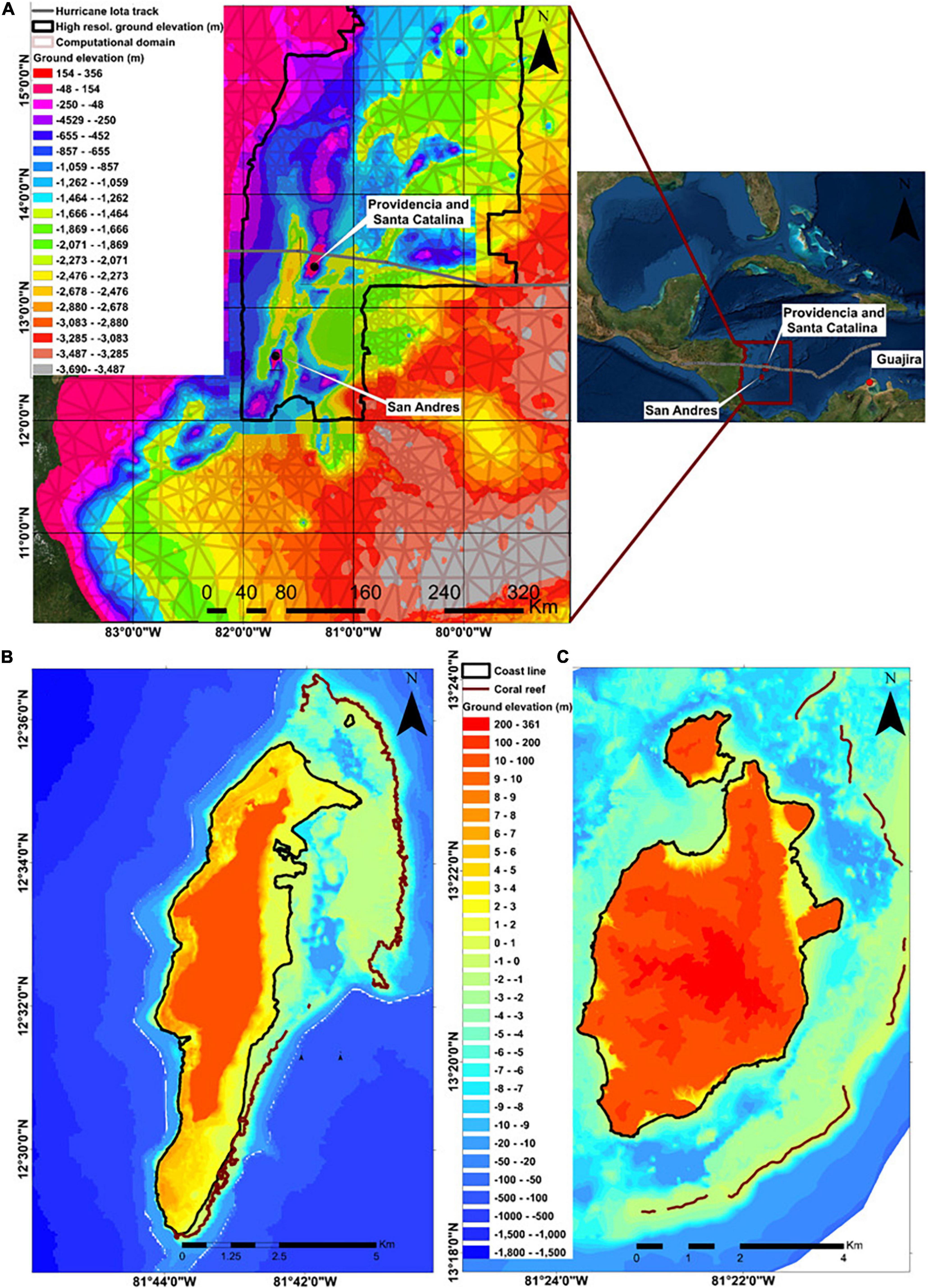
Figure 1. Study area. (A) Topographic elevation and bathymetric depth, computational domain (unstructured mesh), Hurricane Iota track (gray color). Ground elevation data for the islands of (B) San Andres, and (C) Providencia, and Santa Catalina. Santa Catalina is the smallest island located in the north part of Providencia. Modified from Rey et al. (2019b).

Considering the exposure of the SPSC to TC, the archipelago is exposed to hurricane SS flooding, and assessing the inundation hazard is relevant for decision making and planning. Despite the relevance for assessing flood levels, there are only a few historical events to perform a robust statistical description of the TC climate in this area. This limitation has been solved regionally utilizing synthetic TC (Emanuel et al., 2006, 2008) enabling robust statistical analysis to characterize the TC climatology, or using hypothetical TC (Zachry et al., 2015; Rey et al., 2019a) to assess flood worst-case scenarios. In this study, we followed the method from Ruiz-Salcines et al. (2021), using synthetic events (Emanuel et al., 2006, 2008) to develop a model-based hurricane SS flood hazard using a hydrodynamic model. As in previous studies (Lin et al., 2010; Meza-Padilla et al., 2015; Appendini et al., 2019; Marsooli and Lin, 2020), this flood hazard assessment methodology does not rely on historical data on TC or surges, but rather generates synthetic storms that are derived based on the physics of TC (Emanuel et al., 2006, 2008), enabling the assessment of SS flood and their return periods in areas with low TC occurrence, as in the archipelago of SPSC. As such, a large number of synthetic TC were generated over the Caribbean Sea, to use those passing 250 km from the middle point between the San Andres and Providencia islands, and used to force a hydrodynamic model to determine hurricane SS and their associated flood in the archipelago. Additionally, given the scarcity of major hurricanes in the synthetic hurricane dataset, we created hypothetical category V hurricane events for each island to assess the flood worst-case scenario (Zachry et al., 2015; Rey et al., 2019a; Ruiz-Salcines et al., 2021). Considering the above, this study aims to assess the inundation threat from TC for the archipelago of SPSC by means of a hydrodynamic model, which was forced with synthetic tropical cyclones and hypothetical hurricanes, the former to determine the probability for different hurricane SS levels and the latter to provide hurricane SS flood worst-case scenarios. Although the wave contribution to surges in insular environments is significant (Chen et al., 2017), in this study has been neglected due to computational constraints to simulate hundreds of TC events. However, the contribution of the astronomical tide (AT), SS, the wave setup (WS), and wave runup to the maximum seawater level during the pass of hurricane Iota in 2020 for Providencia and Santa Catalina is investigated to know the underestimation of seawater level when waves and tides are not considered. The description of materials and methods as well as description of the study area is introduced in section “Materials and Methods.” The results and discussions are conducted in section “Results and discussions,” and section “Conclusion” presents the main conclusions.

Materials and Methods

Description of the Study Area

The Colombian Caribbean Sea extends from 8° to 13°N latitude and from the country’s border with Panama in the southwest (SW) at longitude 79°W to the Guajira Peninsula in the northeast (NE) at longitude 71° W. The insular Colombian Caribbean is formed by the archipelago of SPSC, the Roncador, Quitasueño, Serrania, and other cays, adjacent islets, and deed-water coral reefs (Otero et al., 2016). The study area is the archipelago of SPSC (Figure 1), composed of the San Andres Island, Providencia, and Santa Catalina and a group of lesser islands, atolls, and coral reefs that are home to a variety of marine flora and fauna (Geister, 1973), making this area the most important tourist destination in Colombia, with roughly 500,000 visitors a year (Ortiz Royero et al., 2015). Figure 1A shows the ground level, which is referred to as the Mean Low Water Spring (MLWS), and the computational domain for the hydrodynamic model.

San Andres is located 190 km east of Nicaragua, and roughly 480 km northwest of the Colombian coast. Providencia is 90 km north of San Andres, and Santa Catalina is separated from Providencia by a 150 m wide channel. The total surface areas for San Andres, Providencia, and Santa Catalina are approximately 2,678 ha, 2,065 ha, and 119 ha, respectively (Rey et al., 2019b). Based on topographic LIDAR data with a spatial resolution of 5 m for the archipelago of SPSC (surveyed from 2010 by the Oceanographic and Hydrographic Research – CIOH, of the General Maritime Direction – DIMAR), the San Andres Island (Figure 1B) is characterized by a low-lying coastal plain in the eastern side with altitudes lower than 5 m, whereas in the western side there is a narrow low-lying area. In the inner sector, there are topographic elevations up to 91 m. The black polygon in Figure 1A represents the bathymetric data collected by CIOH between 2015 and 2017, surveyed with single beam echo sounders in shallow waters and multi-beam echo sounders in deep waters. Outside the polygon, the bathymetric data was complemented with the General Bathymetric Chart of the Oceans (GEBCO) database (International Hydrographic Organization, Intergovernmental Oceanographic Commission) (IHO-IOC, 2018). Figure 1B shows that the insular shelf extends outside the coral reef northeast of San Andres, while the southeast area has a narrow shelf, with corals very close to the coastline or absent. In Providencia Island (Figure 1C), the main low-lying coastal plain area is in the northeast, north, and northwest side. The channel between Santa Catalina and Providencia has average depths of 3 m. The inner sector of Providencia and Santa Catalina have altitudes up to 358 m and 135.6 m, respectively. At the northeast, east, and southeast of Providencia, the insular shelf goes beyond the coral reef.

The Colombian climate is characterized by dry and wet seasons. The former occurs from December to May, and the latter in the rest of the year, interrupted by a relative minimum in June and July known as the Indian summer (Andrade and Barton, 2000). Hurricanes occur from June to November with a peak in activity in September. During most of the wet and dry seasons (September to April), cold fronts generate swells that can create considerable damage to coastal structures (Ortiz et al., 2014). On average there are six cold fronts per year in the Colombian Caribbean zone, but years such as 2010 have presented 20 events, and are relevant for coastal planning as they generate the largest waves in the Colombian Caribbean Sea (Ortiz-Royero et al., 2013), except for the east of the Guajira Peninsula and the archipelago of SPSC where extreme waves are related to TC (Ortiz-Royero, 2012; Otero et al., 2016). During average conditions, the most energetic waves in the continental Colombian Caribbean coast are in the regions of Cartagena, Barranquilla, and Santa Marta while in insular part are in San Andres and Providencia, where stronger trade winds from the northeast generate local sea waves (Osorio et al., 2016).

Tropical Cyclone Datasets Used

To characterize the TC climatology we used synthetic events generated using the method proposed by Emanuel et al. (2006, 2008), consisting of a downscaling technique to allow a better representation of TC in locations with a scarcity of historical events (Emanuel and Jagger, 2010), including gray swan events, which are not be predicted based on history but can have a high-impact and can be foreseeable using physical knowledge together with historical data (Lin and Emanuel, 2016). The TC model involves storm tracks from genesis to lysis. The genesis starts with random seeding of warm-core vortices with peak wind speeds of 12 m/s. These vortices may decay or become TC depending on the ocean and atmospheric environmental conditions. The surviving vortices are then moved by a beta-advection model (Marks, 1992) and intensified based on the Coupled Hurricane Intensity Prediction System (CHIPS) (Emanuel et al., 2004), according to environmental factors based on the National Center for Environmental Prediction/National Center for Atmospheric Research (NCEP/NCAR) reanalysis (Kalnay et al., 1996), referred hereafter as NCEP. The resulting synthetic contained storm parameters such as date, time, position, maximum winds, central pressure, and storm size, which is measured by the radius of maximum wind (R_mw). For this study, we employed a large number of synthetic tracks under NCEP conditions for the late twentieth century (1981–2000) over the Caribbean Sea. The events included 1000 tracks passing within 250 km of the middle point between the San Andres and Providencia islands (81.55° W, 12.95° N). The synthetic hurricane dataset was split into TC categories, from tropical storms to category V hurricanes. These events were used to force a hydrodynamic model to generate SS and determine inundation levels.

The use of a synthetic hurricane dataset allows us to perform robust statistics for TC climate in the area. However, the dataset has only few major hurricanes, with most events being minor hurricanes and tropical storms. As such, the synthetic database limits the determination of the worst-case flood scenario in case of major hurricanes striking the study area. Therefore, we additionally used hypothetical events (to differentiate from synthetic events), which have straight-line trajectories, considering different possible angles of approach to a given site, and different combinations of storm sizes, and forward speeds (Ruiz-Salcines et al., 2021). The hypothetical events we modeled considered category V hurricanes approaching the archipelago of SPSC. The final events had a constant maximum wind speed intensity of 95.17 m/s, a constant forward speed of 5.87 m/s, and a constant R_mw of 56.3 km during their lifetime, for tracks with 11 different approach angles to the area of interest (Figure 2). At the regional level, Hurricane Mitch in 1998 reached category V (79.73 m/s) before making landfall in Honduras, while at a local level, Hurricane Iota in 2020 made landfall in Providencia as category V (72 m/s). Nevertheless, we selected the storm parameters for the hypothetical events based on a conservative perspective of the climatology for this site. Due to the distance between San Andres and Providencia (90 km), we used different hypothetical hurricane datasets for each island. Each of the eleven directions considered three parallel tracks separated by a distance equal to the R_mw, with the central track passing through the center of the island, giving a total of 33 hypothetical events for each island. Figure 2 shows the hypothetical tracks for San Andres and Providencia, the area of movement for hurricane tracks, the computational domain for calculating the hydrodynamic, and the domain for the wind and pressure fields (also used for the synthetic events). The hydrodynamic model was forced with the hypothetical dataset in each island to generate SS to calculate the inundation areas.

FIGURE 2

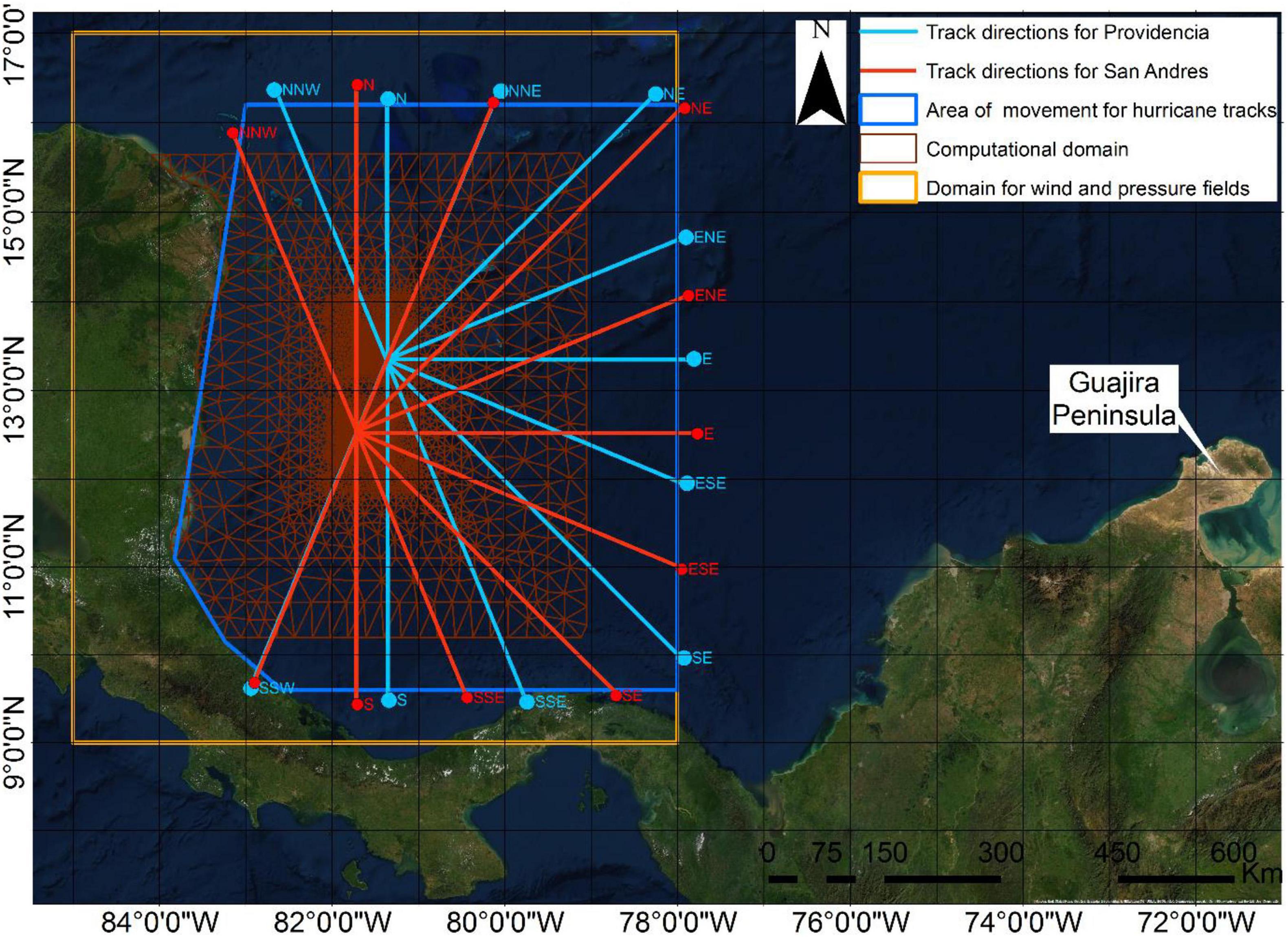
Figure 2. Hypothetical events for San Andres and Providencia. Three parallel tracks per direction were taken into account.

To assess the flooding from Hurricane Iota in 2020 we used storm parameters from the best track dataset from the National Hurricane Center and Central Pacific Hurricane Center (NHC, 2020) to create the input wind fields for the hydrodynamic model.

Hydrodynamic Model Setup

For the hydrodynamic simulations, we used the two-dimensional model MIKE 21 HD FM (DHI, 2014a), which solves the momentum, continuity, temperature, salinity, and density equations with turbulent closure scheme equations. It is based on the incompressible Reynolds averaged Navier-Stokes equations (RANS) under the Boussinesq and hydrostatic pressure approximation (DHI, 2014a). The spatial discretization of the equations was based on the finite volume scheme. The model uses a dynamic time step to optimize simulation speed while ensuring numerical stability and considers a barotropic density with a varying Coriolis force according to the domain. The wetting and drying algorithm is included following the work of Zhao et al. (1994) and Sleigh et al. (1998). The HD FM model used an unstructured mesh (Figure 1) with a resolution of 40 km in the offshore areas far from the islands, increasing its resolution to 80 m in the vicinity of the archipelago and with up to 30 m resolution in the nearshore and flood-prone areas.

Regarding the boundary conditions on the HD FM model, when using the synthetic hurricane dataset, the hydrodynamic model was only forced with wind and pressure fields to account only the TC SS. The computational domain and ocean boundaries were set to zero water level and the boundary along the Nicaraguan coast was set to land. The wind fields were generated at the gradient level by the parametric wind model embedded in the SLOSH hydrodynamic model (Jelesnianski et al., 1992) using the storm characteristics from synthetic and hypothetical TC datasets. This parametric wind model is used by the National Hurricane Center (US) to create wind fields and force the hydrodynamic SLOSH model to forecast hurricane SS inundation in the Gulf of Mexico and the Atlantic ocean (Zachry et al., 2015). As shown by Chen et al. (2019), hybrid wind fields (parametric winds embedded in reanalysis data) provides a better estimation of the tropical cyclone far field winds. While this is not possible for synthetic events, it could be done for historical events such as hurricane Iota (used in this study). Nevertheless, the far field winds are not expected to influence the maximum flood levels in the study area, which is located within the R_mw, thus, the use of parametric wind models is considered more accurate.

The formulation for the parametric wind model is given by

$${\mathit{\text{V}}}_{\mathit{(}\mathit{r}\mathit{)}}={\mathit{\text{V}}}_{\mathit{max}}\frac{\mathit{2}{\mathit{\text{R}}}_{\mathit{mw}}\mathit{\text{r}}}{\mathit{\text{R}}_{\mathit{mw}}{}^{\mathit{2}}+{\mathit{\text{r}}}^{\mathit{2}}}(1)$$

where V_(r) is the gradient wind velocity, at a radius r in m/s, R_mw is the radius of maximum wind in km and V_max is the maximum sustained 1 min speed in m/s.

For TC SS modeling purposes, the wind gradient level requires to be translated to surface level to account for surface friction. The wind correction was done based on the method proposed by Lin and Chavas (2012), and used in other studies (Ruiz-Salcines et al., 2019; Rey et al., 2020). As the model provides symmetric wind fields at gradient level, the translation to surface level provides asymmetric wind fields used to force hydrodynamic models. For the MIKE 21 storm surge simulations, we adjusted the 1-min. wind to a 10-min. average by a reduction factor of 0.893 (Powell et al., 1996). For a given height, wind speed averaged over 10-30 min speeds will typically be about 80% of the maximum 1-min wind speeds (Resio and Westerink, 2008).

The pressure fields were calculated from the pressure distribution model of Holland (1980) as follows, using the storm characteristics from synthetic and hypothetical TC datasets.

$${\mathit{\text{P}}}_{(\mathit{r})}={\mathit{\text{P}}}_{\mathit{c}}+\left({\mathit{\text{P}}}_{\mathit{n}}-{\mathit{\text{P}}}_{\mathit{c}}\right)\text{exp}{\left(-\frac{{\mathit{\text{R}}}_{\mathit{mw}}}{\mathit{\text{r}}}\right)}^{\mathit{B}}(2)$$

where P_c is the central pressure, P_n the ambient pressure, and B is the Holland shape parameter obtained from Eq. 2

$$\mathit{\text{B}}=\frac{\mathit{\text{V}}_{\mathit{max}}{}^{\mathit{2}}\mathit{\text{e}}\mathit{\rho }+{\mathit{\text{fV}}}_{\mathit{max}}{\mathit{\text{R}}}_{\mathit{mw}}\mathit{\text{e}}\mathit{\rho }}{\left({\mathit{\text{P}}}_{\mathit{n}}-{\mathit{\text{P}}}_{\mathit{c}}\right)}(3)$$

where ρ is the air density and e is the base of the natural logarithm.

Regarding Hurricane Iota, we used the approximation given by Silva et al. (2002) (Eq. 4), as the R_mw is not provided by the NHC (2020).

$${\mathit{\text{R}}}_{\mathit{mw}}=\mathbf{0.47}{\mathit{\text{p}}}_{\mathit{c}}-\mathbf{413.01}\left(\mathit{km}\right)(4)$$

where p_c represents the central pressure of the TC. This equation was found by Chang et al. (2015) as the most accurate when compared to other formulations.

When using the hypothetical hurricane dataset, each simulation was run with an initial water level of 0 m and 0.354 m. The latter is the equivalent to the Mean High Water Level (MHWL) as in Rey et al. (2019a) and was calculated from tidal records in San Andres Island covering from January 1997 to February 2015. The tide series have a relative reference and several gaps, which were filled using the Fourier series approximation. Therefore, the gaps were filled before calculating the MHWL. The tidal form factor, or Courtier index (F), obtained was 1.45 and calculated according to the following equation:

$$\mathit{\text{F}}=\frac{{\mathit{\text{K}}}_{\mathbf{1}}+{\mathit{\text{O}}}_{\mathbf{1}}}{{\mathit{\text{M}}}_{\mathbf{2}}+{\mathit{\text{S}}}_{\mathbf{2}}}(5)$$

where K₁, O₁ and M₂ and S₂ are the diurnals (1) and semi-diurnals (2) tide constituents, respectively. In the study area, the tides have a mixed regime, with a predominantly semi-diurnal component (0.25 < F < 1.50), having two high tides and two low tides every day, as defined by Jigena-Antelo et al. (2015).

Because of the tide series gaps, an approximation, based on Fourier series was applied to predict the values of the lost data (Alvera-Azcárate et al., 2005; Bauer et al., 2017). The prediction of missed values of the surface water level (including the residual tide) was reconstructed with the following equation:

$$\begin{array}{l}\mathit{y}(\mathit{t})=\left(\mathbf{0}.\mathbf{1}\mathbf{0}\mathbf{7}*\frac{\mathit{t}}{\mathbf{1}\mathbf{5}\mathbf{4}\mathbf{8}\mathbf{6}\mathbf{5}}-\mathbf{0}.\mathbf{0}\mathbf{5}\right)\\ +\mathit{x}\mathbf{0}+\frac{\mathit{A}}{\mathbf{2}}*\mathit{s}\mathit{i}\mathit{n}\mathit{s}\mathit{i}\mathit{n}(\mathbf{\pi }*\frac{\mathit{t}}{\mathit{a}}+\mathit{\pi })(6)\end{array}$$

where: x0 = 2.38; A = 0.085; a = 30678

This is a procedure that can be applied repeatedly in a cycle until the series converges. Unfortunately, there are no tide gauge records neither in San Andres nor in Providencia during the passing of TC to validate the model results. Therefore, we employed the same model setup as in Rey et al. (2019a, 2020), consisting of a constant eddy viscosity of 0.28 under the Smagorinksy formulation and varying bottom friction based on the Manning coefficients for various categories of land as in previous studies (Mattocks and Forbes, 2008; Zhang et al., 2012). The wind friction varied with the wind speed, as in Rey et al. (2018), with a constant value of 0.001255 for wind speed below 7 m/s and a constant value of 0.002425 for wind speed above 25 m/s, and a linear variation between those values.

For modeling the flood-prone areas derived from Hurricane Iota in Providencia and Santa Catalina, we used four configurations for the model setup: (a) the first to determine SS levels, consisting on forcing the HD FM model with the wind fields from Hurricane Iota over a constant water level set to zero in the computational domain and on the ocean boundaries, (b) the second to account for AT and SS contributions to water levels, where the previous configuration was modified to include tides in the ocean boundaries, as obtained from the tide global model (Andersen, 1995), which represents the major diurnal (K1; O1; P1, and Q1) and semi-diurnal tidal constituents (M2, S2, N2, and K2) with a spatial resolution of 0.25° × 0.25°. Besides the contribution of AT and SS to the water levels, wave runup including both setup and swash (Dorrestein, 1961; Longuet-Higgins and Stewart, 1963; Sallenger, 2000; Stockdon et al., 2007) may be important, particularly for insular environments where the bathymetry is usually quite steep near the coast. Usually, the 2% exceedance level for vertical wave runup (R₂) is used as an indicator of this value (Ruggiero et al., 2001). Therefore, as a first approximation to include the wave contribution to water levels at the coast, we included (c), a third configuration to account for WS contribution by adding wave radiation stresses to configuration (b). To do so, we coupled the HD FM model with the MIKE 21 third-generation Spectral Wave (SW) model (DHI, 2014b). For information regarding source terms of the SW model, governing equations, time integration, and model parameters, readers are referred to Sørensen et al. (2004) and the manual documentation (DHI, 2014b). However, this coupled HD FM – SW model does not take into account the swash contribution to seawater levels. Consequently, a fourth configuration (d) was implemented to solve in detail the coastal processes in the surf zone, such as the wave propagation in shallow water, and the wave runup. As such, we implemented the X Beach 1D model (Roelvink et al., 2010). For validation purposes, we used a bathymetry profile in the eastern part of Santa Catalina (north of Providencia) whose initial point (x = 0.0 m) corresponds to the location of the AW600 sensor (Figure 3), whose recorded data were used as a boundary condition. The last point of the profile (x = 7196 m) ends in the coast, passing through two sensors in x = 3024 m (AW1000) and x = 4008 (RBR), which were used to validate the model. The model was forced with wave parameters (significant wave height Hs, peak wave period Tp, mean wave direction and spectral conditions) and a sea water level recorded by the AW600 sensor.

FIGURE 3

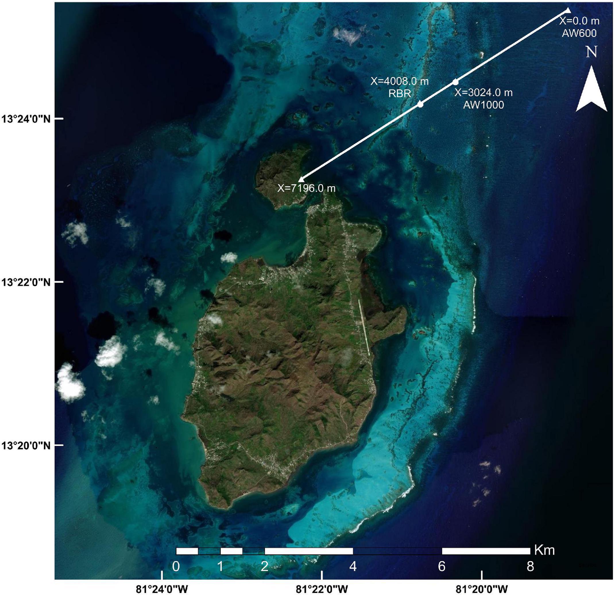
Figure 3. Computational domain for the X Beach model.

For model calibration, we focused on bed friction parameters as this parameter does not change from mean to storm conditions (bed friction due to seafloor configurations). Specifically, we calibrated the values of the bed friction coefficient C_f, which has been used in the same model for similar sea floor configurations (Roelvink et al., 2021), getting values of 0.01 for the points before x = 3600 m and after x = 7090 m, and values of 0.9 in between, where coral rubble can be found (Díaz et al., 2000). According to the seafloor configuration for other profiles, we extrapolated these results to find the zones of the domain where each C_f value applies.

Using the non-hydrostatic mode, from the X Beach profile we extracted the free sea surface elevation every second in the points where the AW1000 and RBR sensors are located. We validated the model by comparing simulated Hs to observations. After validation, we used the same configuration to run the model in profiles located in the eastern and western parts of Providencia. To do so, we forced the X Beach model with wave parameters and water levels obtained from the SW and HD FM models, respectively.

The HD FM model results were processed following the National Hurricane Center (NHC) methodology to obtain the Maximum Envelope of Water (MEOWs) and Maximum of MEOWs (MOMs) (Zachry et al., 2015). The MEOW represents the maximum SS resulting from a set of hypothetical storms of a given category (from tropical storm to category V) and forward speed with varying sizes (related to the R_mw), initial water level, and unique track direction. The MOMs are composed of the maximum SS at each grid/cell element based on the category of storms from all the storm directions, storm sizes, forward speeds, and AT levels (zero or high). It means that MOMs are separated by category and initial water level, retaining the maximum SS value in each grid cell. MEOWs for the synthetic tropical cyclone dataset were not computed because events for a given storm category are allowed to move randomly. There is not a group of parallel synthetic tracks moving in the same direction to reach the coast as in the hypothetical dataset. Therefore, only MOMs for all the categories (tropical storm-category V) for zero tide level were calculated for the synthetic dataset. For the hypothetical dataset, MEOWs and MOMs for hurricane category V were computed for zero and high tide levels.

Extreme Storm Surge Statistical Analysis

The synthetic tropical cyclone dataset is composed of 1000 events. However, we used only events with equal or higher intensity than tropical storms inside a polygon centered in the middle point between San Andres and Providencia and a radius of 250 km. In this sense, only 738 events were considered. The total number of events per category were 366, 256, 49, 36, 22, and 9 for tropical storms, and categories I, II, III, IV, and V, respectively. The surge heights return periods were calculated by combining the SS cumulative distribution function (CDF) and the annual storm frequency (Lin et al., 2010). The SS CDF is estimated based on exceedance statistical methods. Since extreme events usually exhibited a heavy tail, we modeled the tail of the SS CDF using the peaks-over-threshold method (POT) with a generalized Pareto distribution (GPD) and maximum likelihood estimation (Coles, 2001). The threshold values were selected with the criterion of finding the best GPD curve fitting the empirical data.

Results and Discussion

This section shows the 2D MIKE 21 and 1D Xbeach inundation results for Hurricane Iota at Providencia and Santa Catalina, synthetic and hypothetical tropical cyclones inundation maps, as well as the statistical analysis of the synthetic TC SS for the archipelago of San Andres, Providencia and Santa Catalina.

Tide gauge records for San Andres have a mixed tide regime with semidiurnal dominance with strong neap-spring variability, and a tidal range of 1.01 m, varying from 1.90 m during neaps, to 2.91 during springs. The MHWL was calculated based on the Fourier series approximation. Because of the lack of tide gauge records during the pass of TC near San Andres, it was not possible to validate the HD FM model results. However, we used the same calibration parameters used with the hydrodynamic model in previous studies (Rey et al., 2019a, 2020), and we consider this model results reasonable as a first approximation for assessing the inundation threat from tropical cyclones at the study site.

Figure 4 shows hydrodynamic modeling results for the maximum envelope of water depth (i.e., water level above the terrain) induced by Hurricane Iota for Providencia and Santa Catalina, considering the SS contribution (Figure 4A), SS plus AT (Yu et al., 2019), which compose the storm tide (Figure 4B), and storm tide plus WS (Figure 4C). The total flooded area considering only SS was larger than storm tide since Iota passed over Providencia during low tide. The simulation considering storm tide plus WS showed a 14.93 % increase of the flooded area compared to the case when considering only storm tide (an increase of 11.45 ha), similar as in Wu et al. (2018), which used an idealized, alongshore uniform domain, finding that waves have a major influence on the maximum inundation distance inland, with contribution up to 16% of the inundation distance, depending on the different storm characteristics. This significant contribution of the WS to the flood-prone area is because of the bathymetry, which is quite steep beyond the coral reef. Waves make the dominant contribution to the total surge in coastal areas with steep slopes such as near reefed islands or levees. For instance, during typhoon Soudelor in 2015 the wave setup reached up to 0.5–1 m along the northeastern coast of Taiwan (Chen et al., 2017). But even on shallow slopes, the wave contribution could be significant, as an example waves added about 0.6–1.2 m to the surges during Hurricane Katrina in the coast of Louisiana, United States (Resio and Westerink, 2008). Due to computational constraints and the increased computational time when including WS, synthetic and hypothetical events simulations did not include WS, despite the increased flooded area observed under Iota when including WS.

FIGURE 4

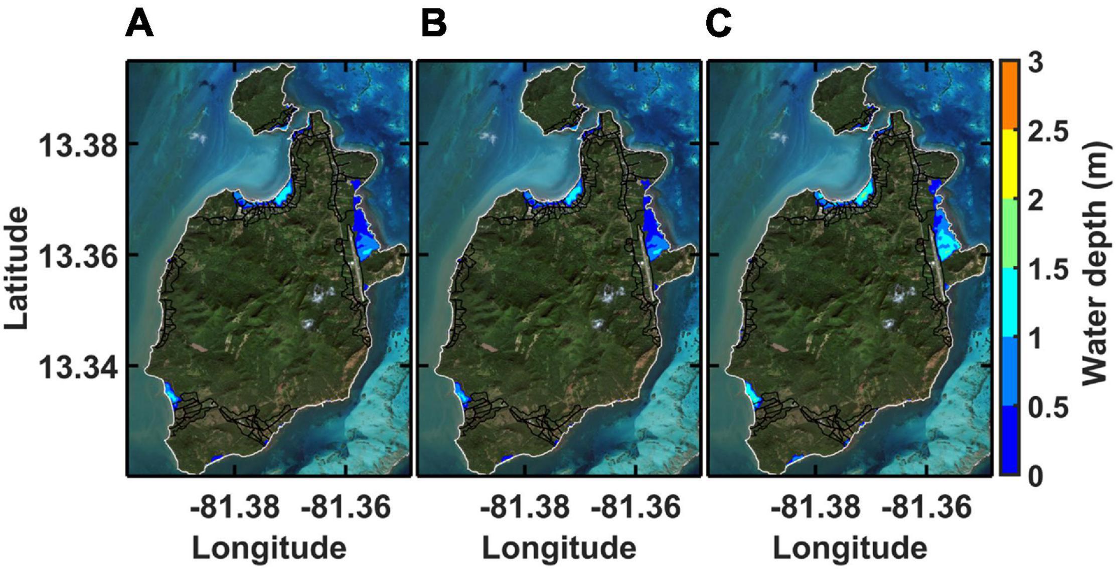
Figure 4. Maximum envelope of water depth induced by Hurricane Iota on Providencia (on the bottom) and Santa Catalina (on the top). The envelope is composed of (A) storm surge, (B) storm tide, (C) storm tide plus wave setup.

Hurricane Iota passed 11 km north of Providencia. Thus, the maximum winds were from offshore north of the island in the forward direction of movement. However, over the island, the winds were in the backward direction of Iota’s track, resulting in the highest flooded water depths northwest of the island. If Iota had passed on the south of Providencia with a distance similar to the R_mw, the hurricane SS would have been larger in the east of the island. Table 1 shows the land area (in hectares, ha) for Providencia and Santa Catalina, as well as the total flooded area induced by hurricane Iota, and flooded area for different water depth intervals and associated percentage related to the total area of each island. The modeled SS induced by Iota on San Andres was negligible (not shown), as Iota passed roughly 100 km to the north.

TABLE 1

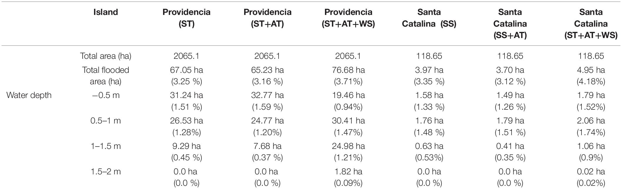
Table 1. Flooded area for Hurricane Iota on Providencia and Santa Catalina.

The previous analysis did not consider the swash contribution to flooding. Therefore, to solve the hydrodynamic details in the surf zone, we modeled the wave propagation in shallow water and the wave runup employing the X Beach 1 D model. Figure 5 presents the Hs and tide levels used as forcing (AW600, Figure 5E) and to validate the X Beach model (AW100 and RBR, Figures 5F,G). Free sea surface levels were recorded at the three sensors between 6/03/2021 at 11h and 15/03/2021 at 15h. The profile and position of the sensors are presented in Figure 5D. The correlation coefficient between the modeled and measured Hs by the AW100 and RBR sensors are 0.93 and 0.80, respectively; and the RMSE are 0.012 m and 0.0025 m, respectively. These results show the capacity of the model to adequately reproduce the hydrodynamics process in the surf zone.

FIGURE 5

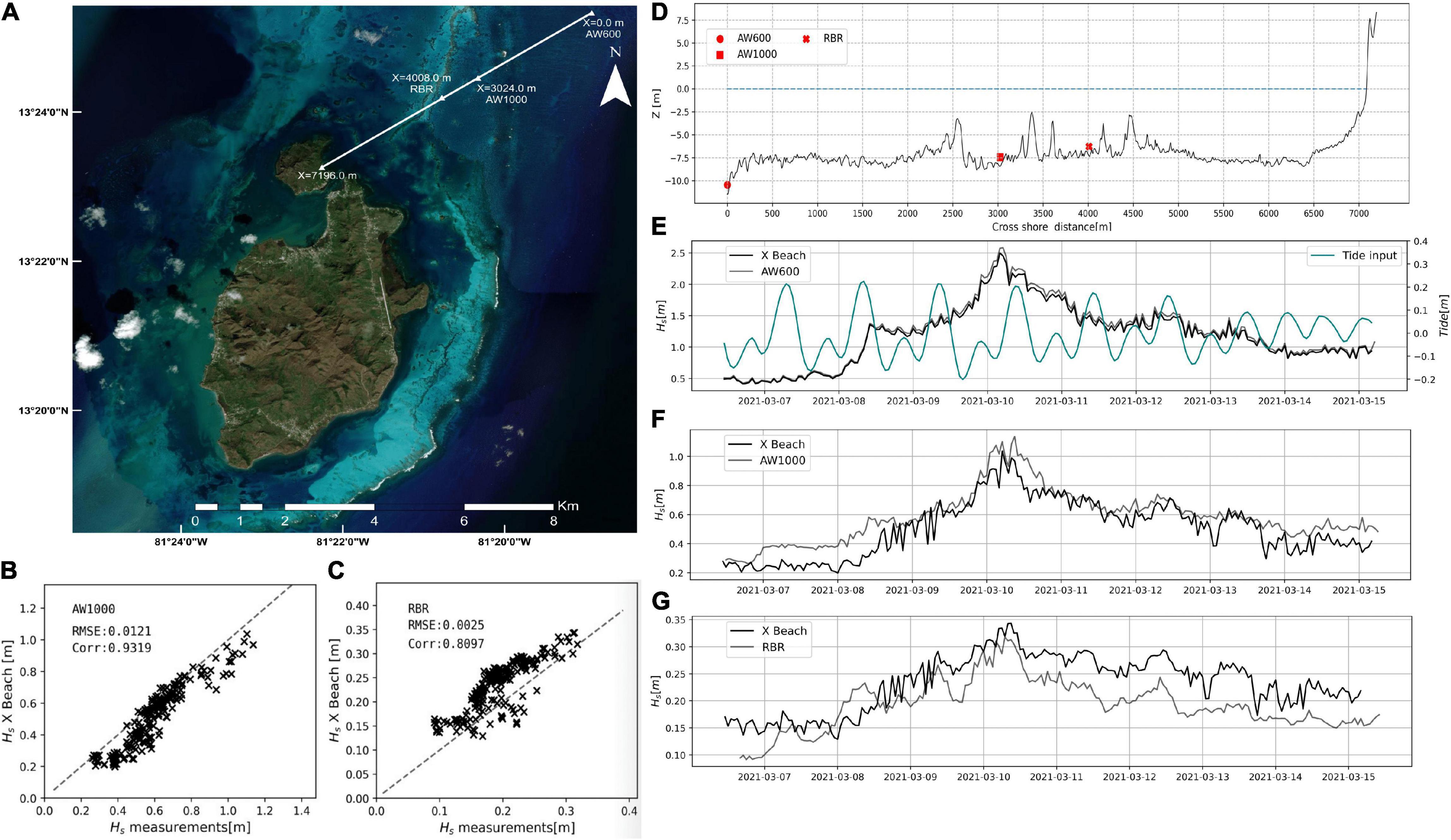
Figure 5. Validation of the X Beach model. (A) Position of the beach profile. (B,C) estimation of the error in the model validation. (D) Position of the sensor on the beach profile. (E) Time series of Hs and tide levels used as forcing in the validation. (F,G) Comparison of the simulated and measured Hs.

Once the X Beach 1D model was validated, we used the model setup for modeling the coastal hydrodynamic in other profiles at Providencia during the pass of Hurricane Iota, specifically at the eastern and western part of the island, where the flood analysis in 2D shows the largest flood-prone areas (Figure 4C). We assessed the contribution of AT, SS, and R₂ to the maximum water level reached, R_high (Sallenger, 2000) (Figure 6), which has vertical and horizontal displacements, varying on each time step. R_high is modulated by SS (Figure 6B). Based on the R_high values at hourly intervals, we estimated the 2% exceedance water level for vertical R_high (R_high2) during the simulation period (42 h). R_high is simulated with the X Beach model, and SS and the storm tide with the HD FM model. R₂ was obtained by subtracting storm tide from R_high2. R_low is composed of storm tide and WS (Sallenger, 2000), simulated with the coupled HD FM – SW model. The WS was estimated by subtracting the modeled storm tide from R_low. Percentage contributions to R_high2 during the storm peak by AT, SS, WS and R₂ were −3.01 %, 46.3 %, 17.17 %, and 56.55 %, respectively (Figure 6C). The negative value is because the AT levels for the storm peak period were low. The spatial evolution of these contributions as well as Hs for the storm peak, using as a reference of the maximum R_high2 (2.22 m) show how the attenuation of Hs is compensated with the increase of SS and WS (Figure 6D). However, the increase of R_high2 is remarkable, with values above 2 m, and this elevation is evident in the swash excursion of around 500 m (Figures 6E,F) inshore. These results confirm oral testimonies of inhabitants and show the importance of wave setup and runup contributions in the flooding process. Finally, Figure 6G shows the percentiles for the simulation period, the storm peak, and the temporal evolution of R_high where the exceedance at 90% is 1.925 m during the storm peak, also confirming the flooding and infrastructure loss in the island during the pass of Hurricane Iota.

FIGURE 6

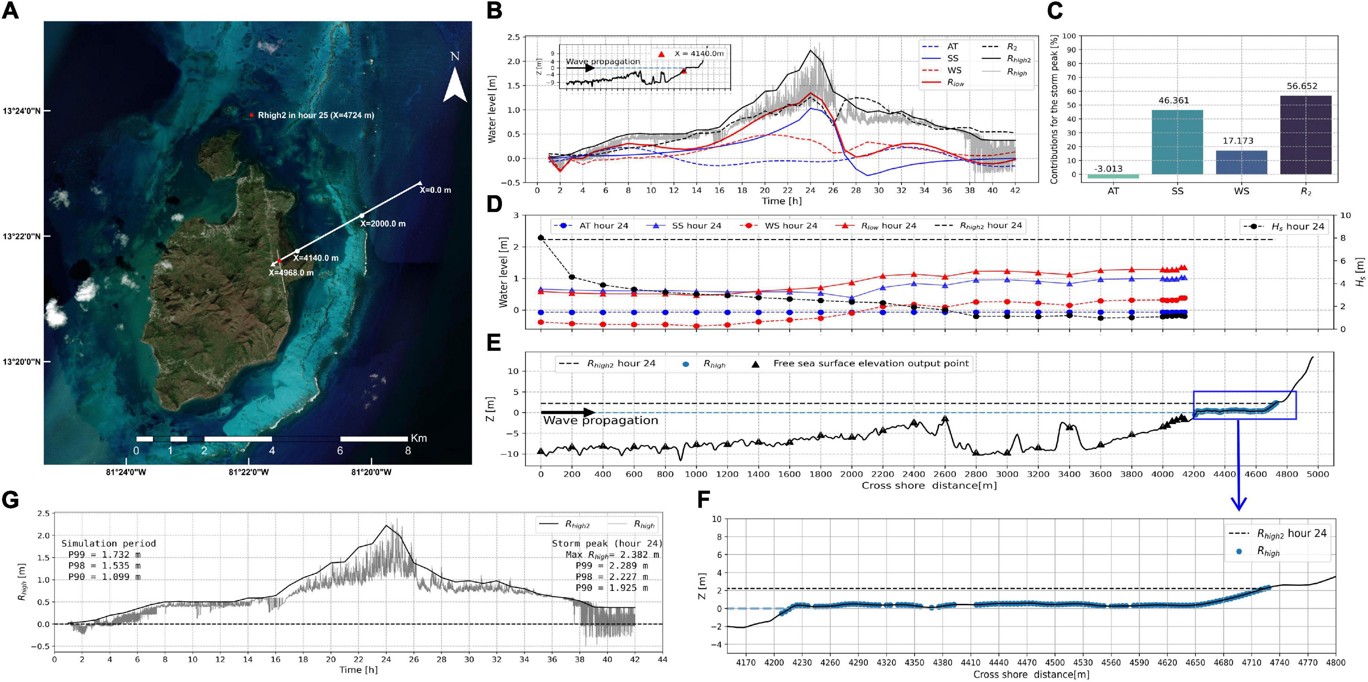
Figure 6. Ocean flood contributions in the eastern side of Providencia during the pass of Iota. (A) Position of the beach profile for analysis of Hurricane Iota flooding. (B) Time series of the water levels for the AT, SS, WS, R₂, R_low, R_high, and R_high2. (C) Percentage contributions to R_high2 by AT, SS, WS and R₂, during the storm peak (24 h). (D) Spatial distribution of AT, SS, WS, R₂, R_low, and R_high2 during the storm peak. (E,F) Horizontal displacements of R_high in the swash excursion. (G) Temporal evolution of R_high.

A similar analysis as the previous one is shown for a profile in the western side of Providencia (Figure 7). The maximum of R_high2 occurred 1 h later than in the eastern part of the island. Due to the location of the profile and the predominant eastern wave direction, the percentage contributions of the AT, SS, WS, and R₂ to R_high2 for the storm peak were −3.56 %, 80.42%, 12.07%, and 23.14%, respectively, which suggests that the SS was the predominant contribution to the maximum seawater level reached on the western side of the island. Therefore, while in the eastern part of Providencia, the predominant contribution to R_high2 was by R₂, in the western was by the SS. The contributions to flood from R₂ and SS are mainly conditioned to the coastal environment such as the bathymetry and configuration of the coast as well as the storm characteristics.

FIGURE 7

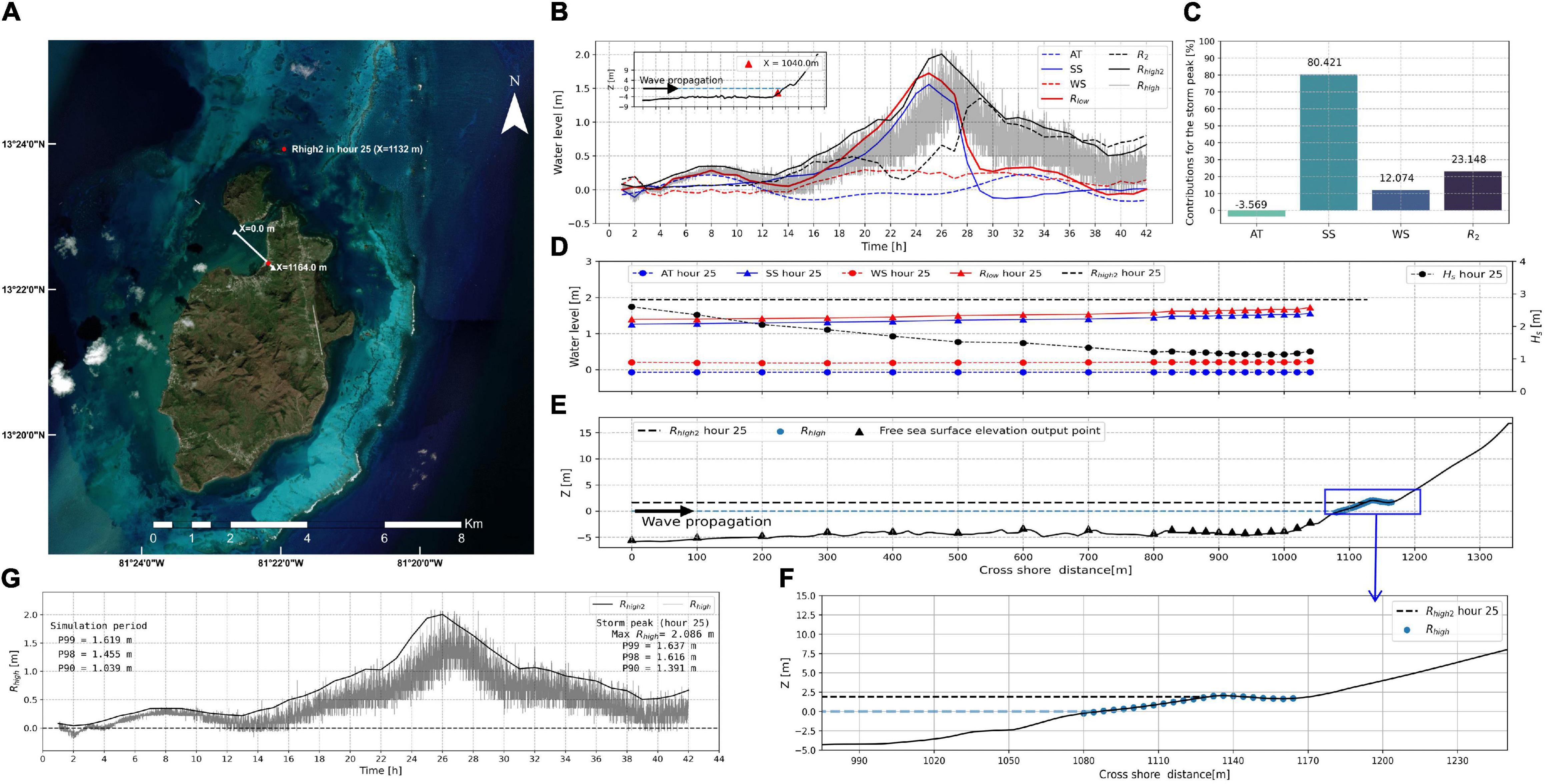
Figure 7. Ocean flood contributions in the western side of Providencia during the pass of Iota. Since this figure shows the same analysis as the previous one, but on the opposite side of the island, the description for each label is the same as for Figure 6.

Figure 8 shows the classification of the synthetic tropical cyclones by category, where each panel shows the entire track of the color-coded events with the category at each track location. Please note that the classification by category is done by using the highest category attained when the event pass inside the red circle, which has a center in the middle point between San Andres and Providencia and a radius of 250 km. As expected, when increasing the hurricane category, the number of events decreases.

FIGURE 8

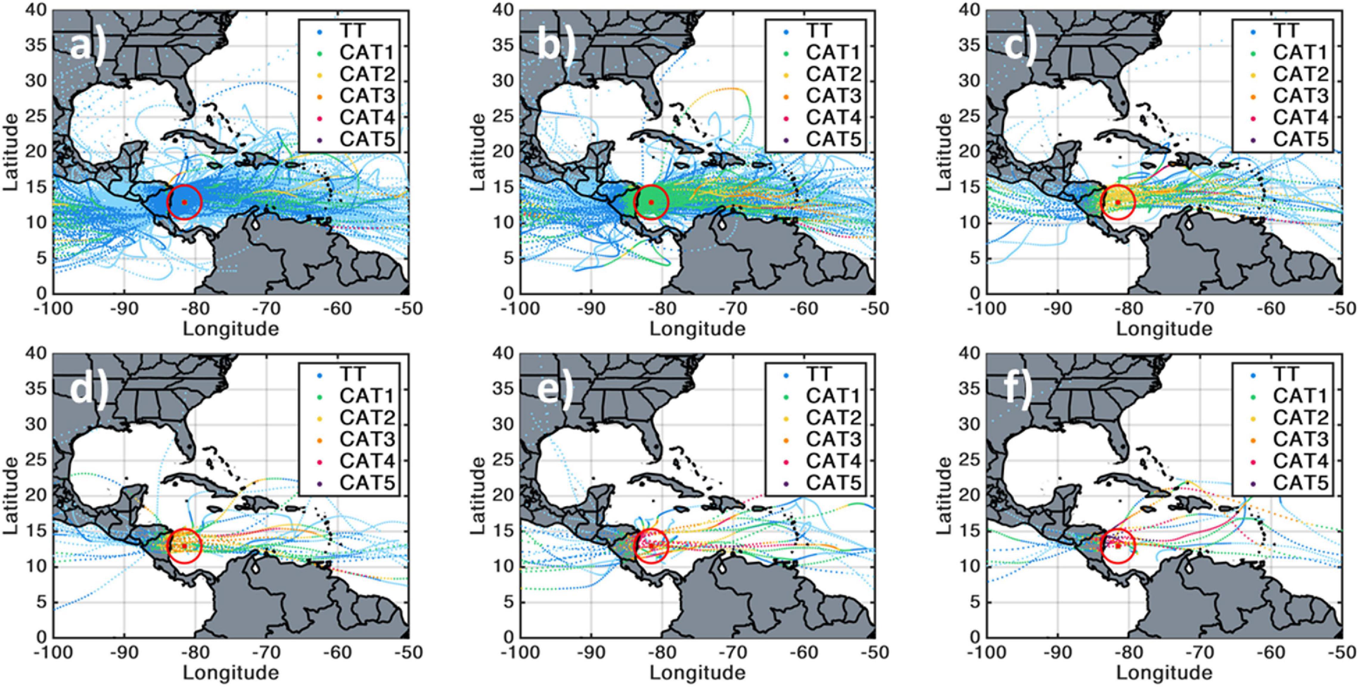
Figure 8. Classification of the synthetic tropical cyclone dataset inside the red polygon. (a) Tropical storms, (b) Hurricane category I, (c) Hurricane category II, (d) Hurricane category III, (e) Hurricane category IV, and (f) Hurricane category V.

Histograms of the simulated SS generated by the synthetic tropical cyclones at San Andres and Providencia islands are shown in Figure 9. The SS values used to create the histograms were extracted for specific points located at sea and inside the computational domain. The coordinates are 81.707° W and 12.5721° N (tide gauge location), and 81.3537° W, 13.3608° N for San Andres and Providencia, respectively. The histogram peaks are approximately at SS level of 0.1 and 0.12 m for San Andres and Providencia, respectively, and rapidly decrease as the values of SS increase, showing a large tail that extends to the maximum SS of 1.68 m and 1.46 m, respectively.

FIGURE 9

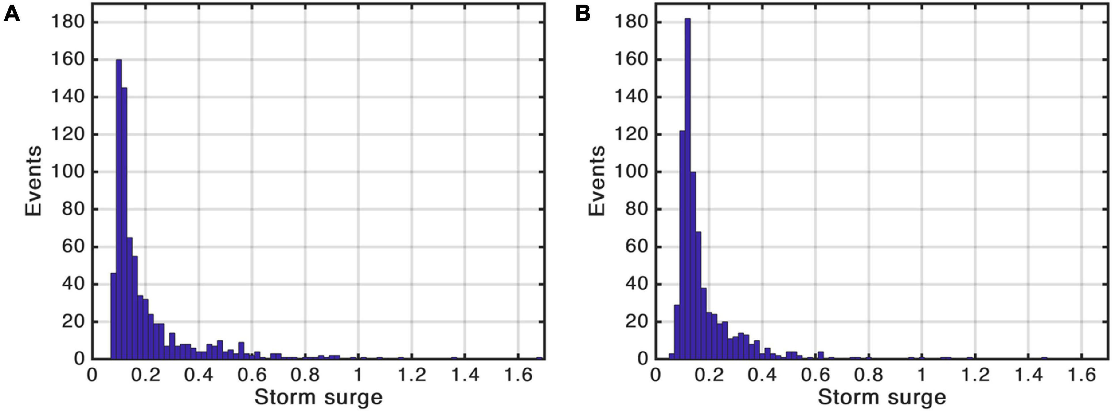
Figure 9. Histograms of the simulated storm surge at the San Andres (A) and Providencia (B) islands for the 738 synthetic tracks that passed within 250 km of the middle point between the San Andres and Providencia Islands.

Figures 10, 11 show synthetic TC MOMs from tropical storm to category V hurricane for zero tide level at San Andres, Providencia, and Santa Catalina, respectively. Each category MOM produces higher SS inundation compared to the corresponding lower category MOM. The city blocks (black lines on the maps) were generated by the National Administrative Department of Statistics of Colombia (DANE, 2018). The results show that the highest exposure area to SS flooding is in the northeast part of San Andres Island, particularly the areas surrounding the harbor and the north part of the island, which is also the most populated area. Other areas do not seem to be exposed to floods, mainly because of their physical characteristics. For instance, while the northeast part of the island has a flat insular shelf and coral reef, which dissipate the waves but amplifies SS (Flather, 2001), the southeast of the island has a narrow shelf with a scarce presence of coral reefs, resulting in negligible SS despite suffering significant wave impact (Ortiz Royero et al., 2015; Bernal et al., 2016). However, the coral barrier reef seems to work as a natural wall that decreases the impact of hurricanes in those islands. The role of the coral reef in inundation, though somehow studied (Gallop et al., 2020), will be a topic of future research for those islands. The total flooded area and associated percentage related to the total area of San Andres are 37.08 ha (1.38%), 52.97 ha (1.97%), 59.55 ha (2.22%), 78.70 ha (2.93%), 95.86 ha (3.57%), and 148.93 ha (5.56 %) for tropical storm, and categories I, II, III, IV, and V, respectively.

FIGURE 10

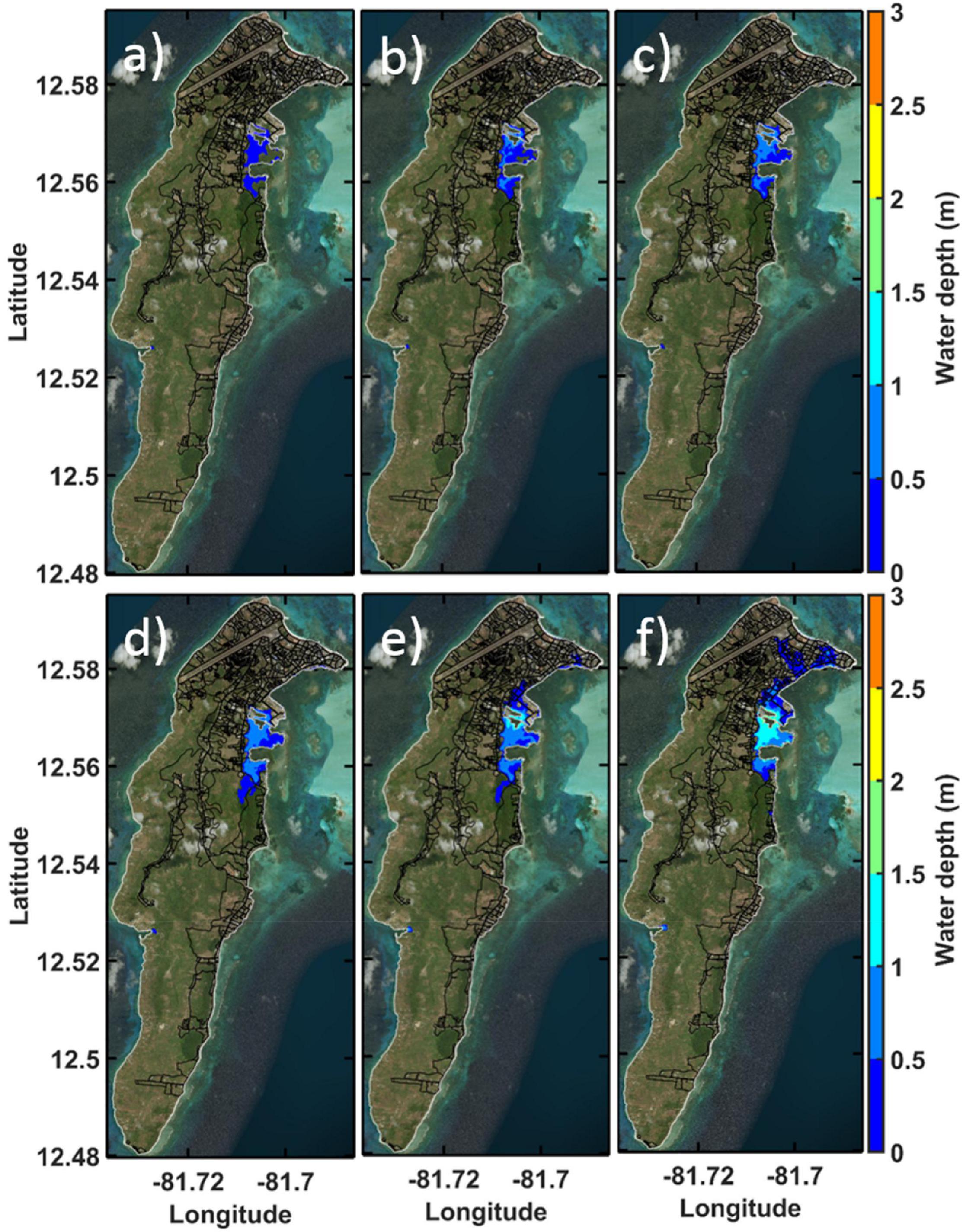
Figure 10. Synthetic hurricane inundation (m) maps for the San Andres Island based on the SSHWS tropical storm to category 5 MOMs product. (a) Tropical storm, (b) category I, (c) category II, (d) category III, (e) category IV, and (f) category V.

FIGURE 11

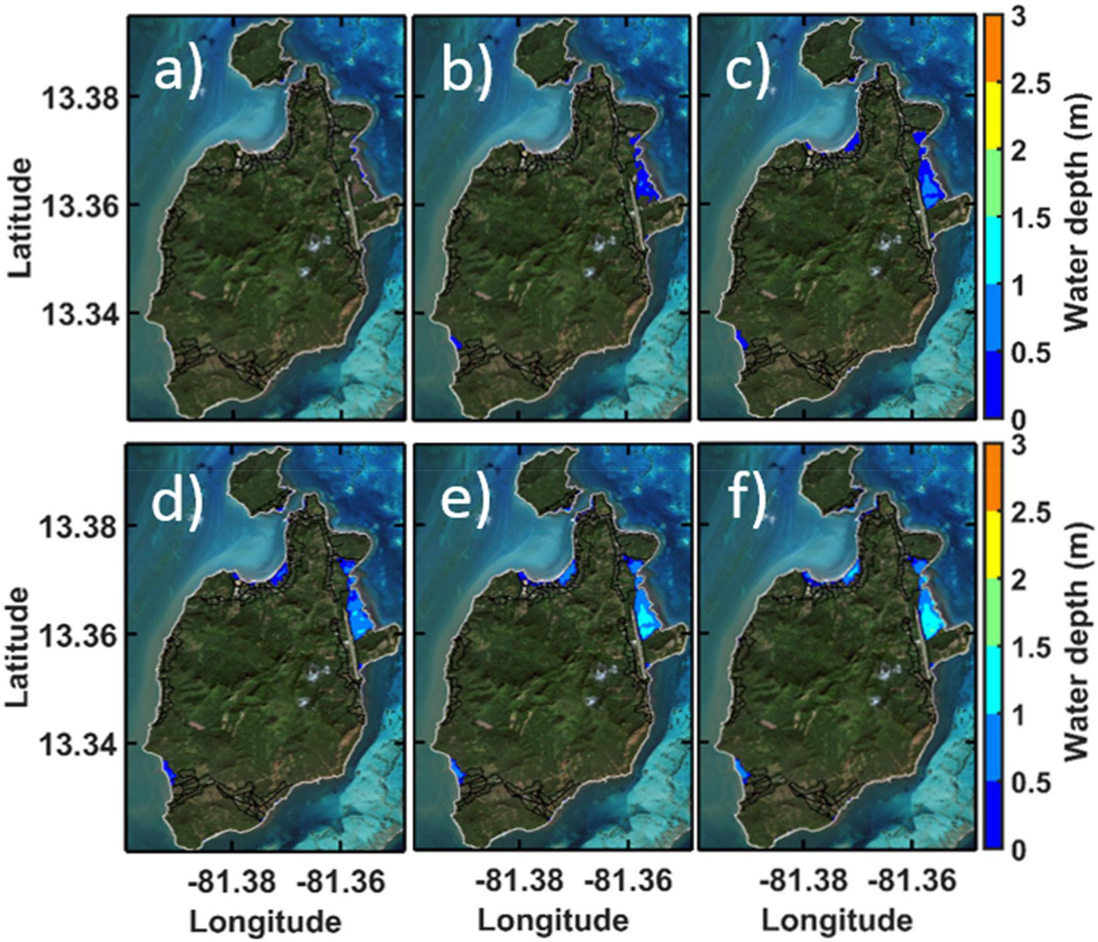
Figure 11. Synthetic hurricane inundation (m) maps for the Providencia and Santa Catalina islands based on the SSHWS tropical storm to category 5 MOMs product. (a) Tropical storm, (b) category I, (c) category II, (d) category III, (e) category IV, and (f) category V.

The northeast of Providencia Island (Figure 11) is the most prone to be flooded because of the flat insular shelf, coral reef, and low topography. Whereas there are no settlements in that area, there is an airport exposed to flooding. For northwest of Providencia, as well as southeast of Santa Catalina, settlements exist in flood-prone areas. The total flooded area and associated percentage related to the total area of Providencia are 3.29 ha (0.15%), 27.32 ha (1.32%), 52.48 ha (2.54%), 58.29 ha (2.82%), 66.49 ha (3.21 %), and 69.30 ha (3.35 %) for tropical storm and categories I, II, III, IV, and V, respectively. These values for Santa Catalina are 0.83 ha (0.7 %), 0.92 (0.78%), 1.64 ha (1.38%), 2.22 ha (1.87%), 2.92 ha (2.46%), and 3.62 ha (3.05%) for tropical storm and categories I, II, III, IV, and V, respectively. The percentage of the flooded area for Providencia derived from the Iota SS is similar to the synthetic hurricane category IV MOM (Figure 11e), and the one generated for Iota SS in Santa Catalina is larger than the synthetic hurricane category V MOM by 8.81% (Figure 11f). Therefore, MOMs based on hypothetical events are important to characterize and cover all susceptible flood-prone areas from TC, which is complicated with synthetic events. More events would be needed.

As an alternative to the lack of enough major hurricanes in the synthetic dataset to assess all the potential exposed areas to hurricane floods, we used hypothetical tracks. This allows assessing the inundation threat for a given area to provide valuable information for evacuation plans. Figure 12 shows the MOMs for hypothetical category V hurricane during (a) low tide and (b) high tide, as well as the flood-prone areas (maximum water depth envelope) induced by the maximum SS resulting from the 738 synthetic tropical cyclones (c) for San Andres. Figures 12d–f shows the same information as described before for Providencia and Santa Catalina. Whereas the hypothetical hurricane category V MOM maps for (a), (b), (d) and (e) in Figure 12 are useful for showing the potential hurricane SS floods, (c) and (f) may not be called MOM because is composed of several synthetic events with different categories, the MOM is composed for events with the same category. However, the information provided in (c) and (f) is useful to determine the probability for different hurricane SS levels. For San Andres, the MOMs show that the maximum water depth is generated around the harbor. This maximum is a result of the diminished flushing capacity through the inlet (Rey et al., 2018). As result, the surrounded area such as the south of the harbor is flooded, this area is characterized as having low altitudes (less than 1 m) and being covered mainly by mangroves. Fortunately, there are just a few houses in that area, at the head of the harbor. The total flooded area and associated percentage related to the total area of San Andres are 354.83 ha (13.24 %), 392.23 ha (14.64%), and 164.63 ha (6.14 %) for the hypothetical hurricane category V MOM for zero tide level, hypothetical hurricane category V MOMs for high tide, and the flood-prone area induced by the synthetic TC SS, respectively. When comparing the flooded area for the hypothetical hurricane category V MOM for zero tide level tide (Figure 12a) with the one for high tide, the latter (Figure 12b) is larger up to 9.53%. It is recommended for future studies to create MEOWs and MOMs based on hypothetical tracks for all the categories (tropical storm to Category V) since synthetic TC dataset is not enough to reproduce the hurricane SS inundation-prone areas. MEOWs and MOMs are used for evacuation plans from a conservative perspective rather than to forecast a single event (Zhang et al., 2013). The flooded area induced by the near-worts-case hypothetical MOM category V for low tide (Figure 12a) is larger up to 53.60 % than the one induced by the synthetic TC events (Figure 12c). As major hurricanes are scarce in the synthetic TC dataset, the use of hypothetical hurricanes provides the opportunity to assess the flooding from higher category events. However, it is important to note that the maximum hurricane SS does not depend only on the hurricane intensity, but also on the storm size, forward speed, direction of approach, and the configuration of the basin and the coastal bathymetry (Resio and Westerink, 2008; Lin et al., 2010).

FIGURE 12

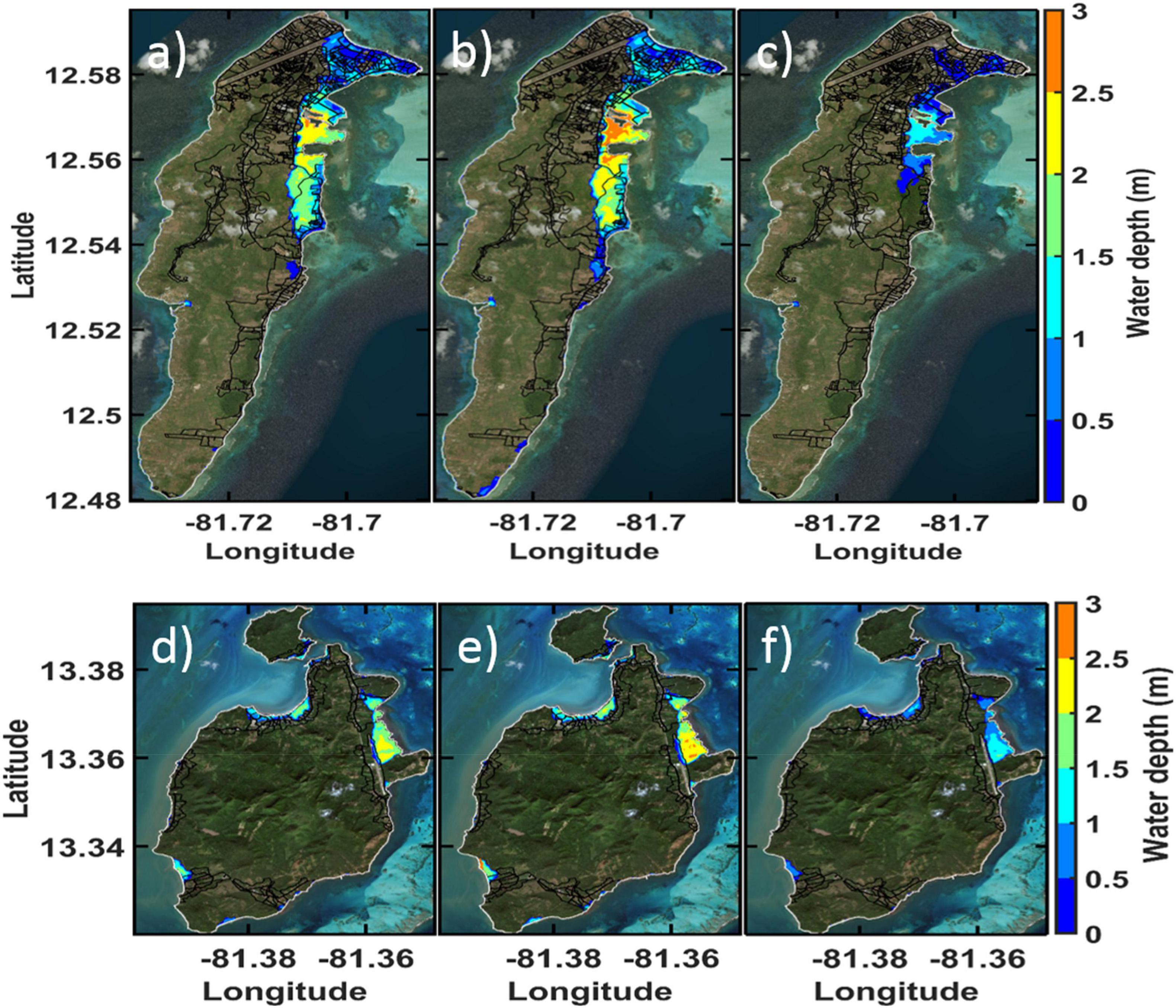
Figure 12. Hurricane inundation (m) maps for San Andres Island (a–c) and Providencia and Santa Catalina Islands (d–f) based on (a,d) the SSHWS hypothetical hurricane category V MOMs for low and, (b,e) high tide, and (c,f) flood-prone area induced by the hurricane SS resulting of the events used from the synthetic TC dataset.

Regarding the total flooded area (Figures 12d–f) and associated percentage related to the total area of Providencia, the values are 91.12 ha (4.41%), 98.57 ha (4.77%), 69.84 ha (3.38 %) for the hypothetical hurricane category V MOM for low tide, and high tide, and for the flood-prone area induced by the synthetic events, respectively. For Santa Catalina, these values are 6.79 ha (5.72 %), 8.89 ha (7.49 %) and 3.62 ha (3.05 %) for the hypothetical hurricane category V MOM for low tide, and high tide, and the flood-prone area induced by the synthetic events, respectively. The flooded area induced by hypothetical hurricane category V MOM for high tide is 7.55%, and 23.62% larger than for low tide for Providencia, and Santa Catalina, respectively.

The main contributors to coastal flooding during the pass of tropical cyclones are the AT, the SS (wind setup plus pressure setup), the wave runup (swash plus wave setup) and the freshwater (river, rainfall). MEOWs and MOMS do not account for the inclusion of wave runup neither freshwater to the total water depth in each hydrodynamic simulation and thus in the MEOWs and MOMs products (Zachry et al., 2015). Additionally, the dynamically forced tidal signal is not included, only a constant water level is considered. Once known these limitations, products from this study may be used adequately.

Another geospatial tool often used for assessing coastal floods is the Geographic Information System (GIS) models. However, the use of hydrodynamic models is preferable to the GIS models for modeling coastal floods (Seenath et al., 2016; Ruiz-Salcines et al., 2021). The latter is primarily based on topography, and it does not take into account the physics of the fluid dynamics (e.g., bottom friction, fluid flow direction, structural barriers). Therefore, in certain cases, it is possible that the use of GIS over-estimates the flood levels and consequently causes over-engineered schemes for defenses and inflated estimates of socio-economic impact. For instance, if the GIS model had been used in this study, all the east parts of San Andres Island from north to south would have been resulted exposed to inundation because the topographic levels are less than 5 m over that zone. However, in the southeast part of the Island, the shelf is narrow with steep slope. Therefore, under these conditions, the SS induced coastal flood is negligible, which is unknown by a GIS model.

Figure 13 shows the hurricane SS return periods for San Andres and Providencia at the same locations used for creating the SS histograms (Figure 9). The thresholds of 0.18 m and 0.14 m were used to define the tail for statistical fitting with the GPD, for San Andres and Providencia, respectively. In order to know the Hurricane Iota SS return period at the location of the extreme analysis at Providencia, we extracted the maximum SS of Iota from the computational domain for that point, which is 1.25 m. Thus, looking into the SS return period curve for Providencia, this value has an associate return period of 3,234-years (Figure 13B). Given the low probability of the Hurricane Iota SS under present climate, future studies should consider the effect of climate change on tropical cyclones (Lin et al., 2019; Marsooli and Lin, 2020) to know if storm surge values as the one for Hurricane Iota will be more frequent in Providencia and Santa Catalina at the end of the century.

FIGURE 13

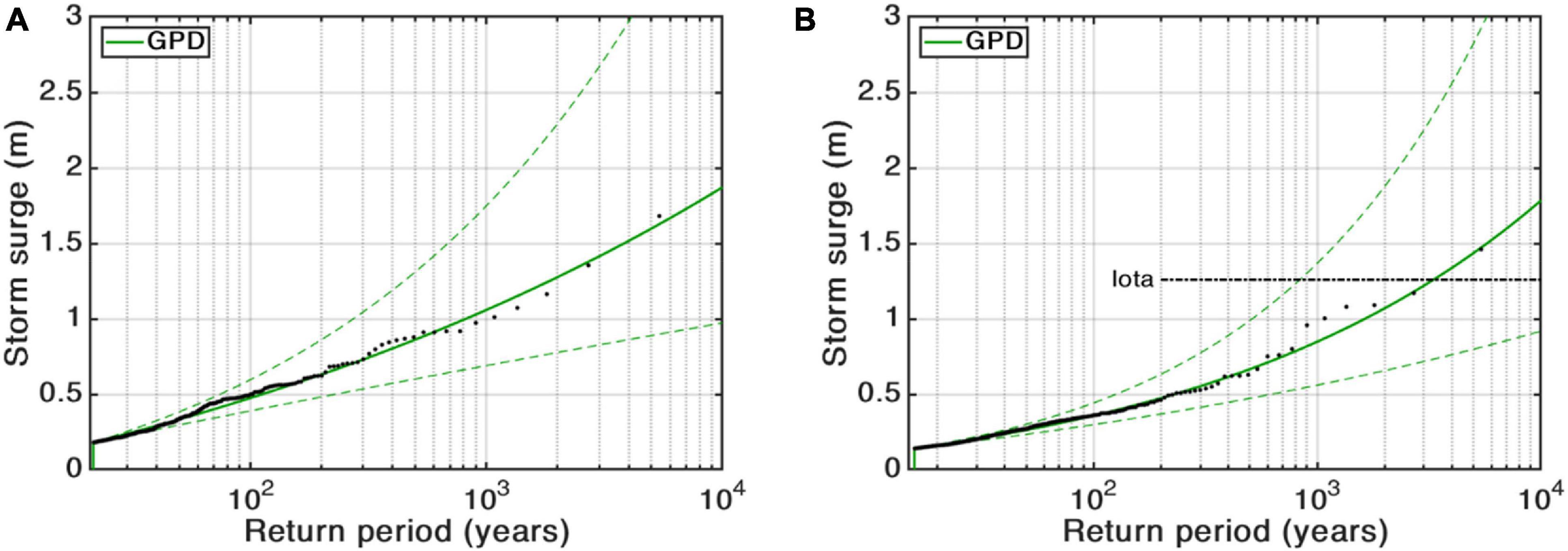
Figure 13. Storm surge return periods for (A) San Andres, (B) Providencia. The green solid curve is the mean return level and the green dashed curves are the 95% confidence limits. The black points are the empirically estimated storm surge return levels.

Based on the water depth induced by the synthetic TC events, we estimated the 100-year (Figures 14a,b) and 500-year (Figures 14c,d) return periods for San Andres, Providencia, and Santa Catalina. From each element of the computational domain on the flooded area, we extracted the water depth associated with 100-year and 500-year return periods. This analysis was done based on the empirical estimated water depth return levels. It means that the water depth at each element was not fitted to a canonical probability distribution. The water depth heights return periods were calculated by combining the water depth heights CDF and the annual storm frequency. Whereas water depth levels associated with 100-years return periods cover partially the east part of these islands, the 500-years return periods increase significantly the flooded area around the harbor and the airport for San Andres and Providencia, respectively. Flooded areas outside of the 500-years flood return period map, such as the ones shown in previous figure (Figures 12c,f), have larger return periods. It means that the water depth levels on the north of San Andres have return periods larger than 500 years.

FIGURE 14

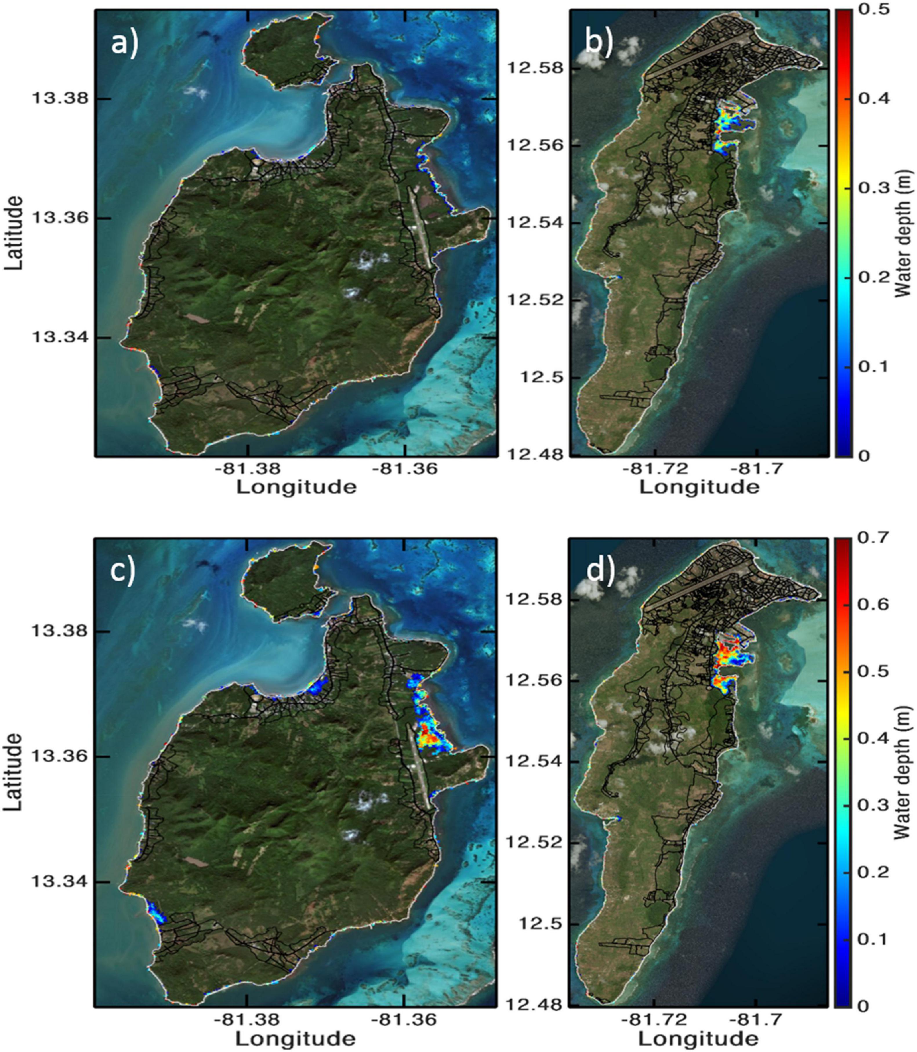
Figure 14. 100-year (a,b) and 500-years (c,d) water depth return period maps for (a,c) Providencia and Santa Catalina, and (b,d) San Andres.

The use of synthetic or hypothetical datasets to do flood hazard assessments depends on the objective of the study. As such, synthetic events provide a robust dataset for statistical analysis to characterize present and future climate trends, whereas hypothetical events allow assessing the inundation threat, which is very useful for evacuation plans from a conservative perspective (Rey et al., 2019a), and also for estimating the near-worst-case flood scenario, including climate change (Ruiz-Salcines et al., 2021). For coastal environments with steep slopes, the contribution of waves may be larger or equal than SS to flooding (Stockdon et al., 2007; Chen et al., 2017) while in wide and shallow continental shelf with a mild slope (e.g., continental shelf for Yucatan in the Gulf of Mexico) this behavior is inverted (Rey et al., 2020).

Conclusion

This study presents a characterization of the hurricane SS inundation threat for the archipelago of San Andres, Providencia, and Santa Catalina, which is a site with scarce historical events. SS was investigated using a hydrodynamic model forced with synthetic tropical cyclones and hypothetical hurricanes. The former are mathematical events derived using hurricane physics useful to determine the probability for different hurricane SS levels and the latter are events with category V hurricanes during all their lifetime and with different track direction toward the archipelago to establish the near-worst-case hurricane SS flood scenarios. The use of synthetic events allowed us to perform statistical analysis of hurricane SS heights at San Andres, Providencia and Santa Catalina. This analysis suggested that the eastern part of San Andres is more likely to be flooded from hurricanes SS than the north, and for Providencia the east is more likely to be flooded than the northwest. The hypothetical category V hurricane MOMs for high tide show the worst-case flood scenario from hurricanes SS and a constant water level associated with the MHWL. In this sense, the flooded area and associated percentage related to the total area of San Andres, Providencia, and Santa Catalina are 392.23 ha (14.64%), 98.57 ha (4.77%), 8.89 ha (7.49 %), respectively. This is because of the role that plays the flat insular shelf and coral reef, which would be the topic of a future study. Additionally, we modeled the Hurricane Iota (2020) inundation for Providencia with 2 D and 1 D models. For the former we considered contributions from SS, AT, and WS. The flooded area derived from these three contributions was 75.93 ha, which represents 3.68% of the island. The contribution of the wave setup was 14.93 % (11.45 ha) of the total flooded area modeled. For the latter, modeling results with X-beach (1 D) in the eastern side of the island showed that the AT, SS, and R₂ contribution to the maximum water level reached -3.01%, 46.36%, and 56.55 %, respectively during the storm peak. This information provided an approximation of the underestimation of the seawater level when modeling only SS without including the wave contribution through the WS and swash in insular environments. The maximum SS derived from Hurricane Iota for the east of Providencia was 1.25 m, which according to this study has an associated return period of 3,234-years. Therefore, future studies should consider the effect of climate change on tropical cyclones to know if the probability of storm surge values as the one for Hurricane Iota may be increased in Providencia Island with the current global warming trends. This methodology may be applied to other coastal zones and extended to consider the effect of climate change on hurricane SS and the sea level rise, which together with the increase of settlements along coastal zones will increase the flood risk by the end of the century. This study provides tools for decision-makers to implement initiatives to make those islands more resilient.

Data Availability Statement

The original contributions presented in the study are included in the article/supplementary material, further inquiries can be directed to the corresponding authors.

Author Contributions

WR, PR-S, PS, AFO, JPR, BJ-A, and CMA: conceptualization and methodology. WR, PR-S, JPR, and BJ-A : software. WR, PR-S, and JPR: validation and visualization. WR, PR-S, JPR, BJ-A, and AFO: formal analysis. WR, CMA, PR-S, CPU-L, GE-O, and AC-M: investigation. WR, PS, CPU-L, GE-O, and CMA: resources. WR, PR-S, AFO, and JPR: data curation. WR, AFO, BJ-A, and CMA: writing—original draft preparation. WR, PR-S, PS, AFO, JPR, BJ-A, CPU-L, GE-O, AC-M, and CMA: writing—review and editing. WR, CMA, and AFO: supervision and project administration. PS, CPU-L, GE-O, AC-M, and CMA: funding acquisition. All authors contributed to manuscript revision, read, and approved the submitted version.

Funding

WR was funded by the Council of the National Research Training (COLCIENCIAS) through the postdoctoral internship program number 784, DIMAR with projects 236-SUBAFIN-2018, 110-SUBAFIN-2019, GINRED4-2020, and the Mexican National Coastal Resilience Laboratory (LANRESC). This work was funded by COLCIENCIAS, DIMAR-CIOH, and partially by the Centro Mexicano de Innovación en Energia del Oceano, CEMIE-Oceano (OLE-1). AFO and JPR acknowledge the data provided by the project Convenio 003 de 2020 CORALINA-UNAL, “Estudio para definir el riesgo por inundación en la isla de San Andres, ante huracanes en las categorías más probables”.

Conflict of Interest

The authors declare that the research was conducted in the absence of any commercial or financial relationships that could be construed as a potential conflict of interest.

Publisher’s Note

All claims expressed in this article are solely those of the authors and do not necessarily represent those of their affiliated organizations, or those of the publisher, the editors and the reviewers. Any product that may be evaluated in this article, or claim that may be made by its manufacturer, is not guaranteed or endorsed by the publisher.

Acknowledgments

WR thanks Gonzalo U. Martín-Ruiz, Fernando Afanador-Franco, Julio Monroy, Emerson Herrera-Vásquez, Julian Quintero-Ibáñez, and Juan David Santana-Mejia for their help with computer resources, technical support, and data acquisition. Finally, we gratefully acknowledge Kerry Emanuel from Massachusetts Institute of Technology for providing the synthetic hurricane dataset for this study and to Alec Torres-Freyermuth for his comments to improve this manuscript.

References

Alvera-Azcárate, A., Barth, A., Rixen, M., and Beckers, J. M. (2005). Reconstruction of incomplete oceanographic data sets using empirical orthogonal functions: application to the Adriatic Sea surface temperature. Ocean Model. 9, 325–346. doi: 10.1016/j.ocemod.2004.08.001

CrossRef Full Text | Google Scholar

Andersen, O. B. (1995). Global ocean tides from ERS 1 and TOPEX/POSEIDON altimetry. J. Geophys. Res. 100, 25249–25259.

Google Scholar

Andrade, C. A., and Barton, E. D. (2000). Eddy development and motion in the Caribbean Sea. J. Geophys. Res. Ocean 105, 26191–26201. doi: 10.1029/2000jc000300

CrossRef Full Text | Google Scholar

Appendini, C. M., Meza-padilla, R., Abud-russell, S., Proust, S., Barrios, R. E., and Secaira-Fajardo, F. (2019). Effect of climate change over landfalling hurricanes at the Yucatan Peninsula. Clim. Change 157, 1–14. doi: 10.1007/s10584-019-02569-5

CrossRef Full Text | Google Scholar

Bauer, J., Angelini, O., and Denev, A. (2017). Imputation of multivariate time series data - performance benchmarks for multiple imputation and spectral techniques. SSRN Electron. J. XXI, 1–5. doi: 10.2139/ssrn.2996611

CrossRef Full Text | Google Scholar

Bernal, G., Osorio, A. F., Urrego, L., Peláez, D., Molina, E., Zea, S., et al. (2016). Occurrence of energetic extreme oceanic events in the Colombian Caribbean coasts and some approaches to assess their impact on ecosystems. J. Mar. Syst. 164, 85–100. doi: 10.1016/j.jmarsys.2016.08.007

CrossRef Full Text | Google Scholar

CCO (2015). Mapa Esquemático de Colombia. In: Colomb. Goverment. Available online at: http://www.cco.gov.co/cco/publicaciones/83-publicaciones/262-mapa-esquematico-de-colombia.html (accessed May 28, 2020).

Google Scholar

Chang, C. H., Shih, H. J., Chen, W. B., Su, W. R., Lin, L. Y., Yu, Y. C., et al. (2018). Hazard assessment of typhoon-driven storm waves in the nearshore waters of Taiwan. Water 10:926. doi: 10.3390/w10070926

CrossRef Full Text | Google Scholar

Chang, C. M., Fang, H. M., Chen, Y. W., and Chuang, S. H. (2015). Discussion on the maximum storm radius equations when calculating typhoon waves. J. Mar. Sci. Technol. 23, 608–619. doi: 10.6119/JMST-015-0226-1

CrossRef Full Text | Google Scholar

Chen, W.-B., Chen, H., Hsiao, S.-C., Chang, C.-H., and Lin, L.-Y. (2019). Wind forcing effect on hindcasting of typhoon-driven extreme waves. Ocean Eng. 188:106260. doi: 10.1016/j.oceaneng.2019.106260

CrossRef Full Text | Google Scholar

Chen, W. B., Lin, L. Y., Jang, J. H., and Chang, C. H. (2017). Simulation of typhoon-induced storm tides and wind waves for the northeastern coast of Taiwan using a tide-surge-wave coupled model. Water 9:549. doi: 10.3390/w9070549

CrossRef Full Text | Google Scholar

Coles, S. (2001). An Introduction to Statistical Modeling of Extreme Values. London: Springer.

Google Scholar

DANE (2018). Geoportal DANE – Descarga del Marco Geoestadistico Nacional (MGN). Available online at: https://geoportal.dane.gov.co/ (accessed October 3, 2020).

Google Scholar

DHI (2014a). MIKE 21 Toolbox: Global Tide Model-Tidal Prediction. Hoersholm: DHI Water & Environment, 20.

Google Scholar

DHI (2014b). MIKE 21 SW: Spectral Waves FM Module, User Guide. Hoersholm: DHI Water & Environment, 122.

Google Scholar

Díaz, J., Barrios, L., Cendales, M., Garzón-Ferreira, J., Geister, J., López-Victoria, M., et al. (2000). Áreas Coralinas de Colombia. No 5. Santa Marta: INVEMAR Ser Publicaciones, 176.

Google Scholar

Dorrestein, R. (1961). “Wave set-up on a beach,” in Proceedings of the 2nd Tech. Conf. on Hurricanes, Miami Beach, FL., Nat. Hurricane Res. Proj. Rep. 50 (Washington, DC: US Dept. of Commerce), 230–241.

Google Scholar

Emanuel, K., DesAutels, C., Holloway, C., and Korty, R. (2004). Environmental control of tropical cyclone intensity. J. Atmos. Sci. 61, 843–858. doi: 10.1175/1520-04692004061<0843:ECOTCI<2.0.CO;2

CrossRef Full Text | Google Scholar

Emanuel, K., and Jagger, T. (2010). On estimating hurricane return periods. J. Appl. Meteorol. Climatol. 49, 837–844. doi: 10.1175/2009JAMC2236.1

CrossRef Full Text | Google Scholar

Emanuel, K., Ravela, S., Vivant, E., and Risi, C. (2006). A statistical deterministic approach to hurricane risk assessment. Bull. Am. Meteorol. Soc. 87, 299–314. doi: 10.1175/BAMS-87-3-299

CrossRef Full Text | Google Scholar

Emanuel, K., Sundararajan, R., and Williams, J. (2008). Hurricanes and global warming: results from downscaling IPCC AR4 simulations. Bull. Am. Meteorol. Soc. 89, 347–367. doi: 10.1175/BAMS-89-3-347

CrossRef Full Text | Google Scholar

Faust, E., and Bove, M. (2017). The Hurricane Season 2017: A Cluster of Extreme Storms. MunichRE. Available online at: https://www.munichre.com/topics-online/en/climate-change-and-natural-disasters/natural-disasters/storms/hurricane-season-2017.html#experts (accessed May 25, 2020).

Google Scholar

Flather, R. A. (2001). “Storm surges,” in Encyclopedia of Ocean Sciences, eds J. H. Steele, S. A. Thorpe, and K. K. Turekian (San Diego, CA: Academic Press), 2882–2892.

Google Scholar

Gallop, S. L., Kennedy, D. M., Loureiro, C., Naylor, L. A., Muñoz-Pérez, J. J., Jackson, D. W. T., et al. (2020). Geologically controlled sandy beaches: their geomorphology, morphodynamics and classification. Sci. Total Environ. 731:139123. doi: 10.1016/j.scitotenv.2020.139123

PubMed Abstract | CrossRef Full Text | Google Scholar

Geister, J. (1973). Los Arrecifes de la Isla De San Andrés (Mar Caribe, Colombia). Mitt. Inst. Colombo Alemán Invest. Cient. 7, 211–228. doi: 10.25268/bimc.invemar.1973.7.0.553

CrossRef Full Text | Google Scholar

Holland, G. J. (1980). An analytical model of the wind and pressure profiles in hurricanes. Mon. Weather Rev. 108, 1212–1218.

Google Scholar

IHO-IOC (2018). A Technical Reference Manual on How to Build Bathymetric Grids. IHO Publ. B-11. Available online at: https://www.gebco.net/data_and_products/gebco_cook_book/ (accessed March 26, 2021).

Google Scholar

Jelesnianski, C., Chen, J., and Shaffer, W. (1992). SLOSH: Sea, Lake, and Overland Surges from Hurricanes. NOAA Technical Report NWS 48. Miami, FL: United States Department Commerce NOAA/AOML Library.

Google Scholar

Jigena-Antelo, B., Vidal, J., and Berrocoso, M. (2015). Determination of the tide constituents at Livingston and deception Islands (South Shetland Islands, Antarctica), using annual time series. Dyna 82, 209–218. doi: 10.15446/dyna.v82n191.45207

CrossRef Full Text | Google Scholar

Kalnay, E., Kanamitsu, M., Kistler, R., Collins, W., Deaven, D., Gandin, L., et al. (1996). The NCEP/NCAR 40-year reanalysis project. Bull. Am. Meteorol. Soc. 77, 437–471.

Google Scholar

Lin, N., and Chavas, D. (2012). On hurricane parametric wind and applications in storm surge modeling. J. Geophys. Res. Atmos. 117, 1–19. doi: 10.1029/2011JD017126

CrossRef Full Text | Google Scholar

Lin, N., and Emanuel, K. (2016). Grey swan tropical cyclones. Nat. Clim. Change 6, 106–111. doi: 10.1038/nclimate2777

CrossRef Full Text | Google Scholar

Lin, N., Emanuel, K. A., Smith, J. A., and Vanmarcke, E. (2010). Risk assessment of hurricane storm surge for New York City. J. Geophys. Res. 115:D18121. doi: 10.1029/2009JD013630

CrossRef Full Text | Google Scholar

Lin, N., Lane, P., Emanuel, K. A., Sullivan, R. M., and Donnelly, J. P. (2014). Heightened hurricane surge risk in northwest Florida revealed from climatological-hydrodynamic modeling and paleorecord reconstruction. J. Geophys. Res. Atmos. 119, 8606–8623. doi: 10.1002/2014JD021584

CrossRef Full Text | Google Scholar

Lin, N., Marsooli, R., and Colle, B. A. (2019). Storm surge return levels induced by mid-to-late-twenty-first-century extratropical cyclones in the Northeastern United States. Clim. Change 154, 143–158. doi: 10.1007/s10584-019-02431-8

CrossRef Full Text | Google Scholar

Longuet-Higgins, M. S., and Stewart, R. (1963). A note on wave set-up. J. Mar. Res. 21, 4–10.

Google Scholar

Marks, D. G. (1992). The Beta and Advection Model for Hurricane Track Forecasting. Camp Springs, MD: NOAA Technical Memorandum NWS NMC 70.

Google Scholar

Marsooli, R., and Lin, N. (2020). Impacts of climate change on hurricane flood hazards in Jamaica Bay, New York. Clim. Change 163, 2153–2171. doi: 10.1007/s10584-020-02932-x

CrossRef Full Text | Google Scholar

Martell-Dubois, R., Silva-Casarin, R., Mendoza-Baldwin, E. G., Muñoz-Pérez, J. J., Cerdeira-Estrada, S., Escalante-Mancera, E., et al. (2018). Bimodalidad espectral del oleaje provocado por huracanes en la zona costera del caribe Mexicano. Cien. Mar. 44, 33–48. doi: 10.7773/cm.v44i1.2717

CrossRef Full Text | Google Scholar

Mattocks, C., and Forbes, C. (2008). A real-time, event-triggered storm surge forecasting system for the state of North Carolina. Ocean Model. 25, 95–119. doi: 10.1016/j.ocemod.2008.06.008

CrossRef Full Text | Google Scholar

Mendoza, E., Velasco, M., Velasco-Herrera, G., Martell, R., Silva, R., Escudero, M., et al. (2020). Spectral analysis of sea surface elevations produced by big storms: the case of hurricane Wilma. Reg. Stud. Mar. Sci. 39:101390. doi: 10.1016/j.rsma.2020.101390

CrossRef Full Text | Google Scholar

Meza-Padilla, R., Appendini, C. M., and Pedrozo-Acuña, A. (2015). Hurricane-induced waves and storm surge modeling for the Mexican coast. Ocean Dyn. 65, 1199–1211. doi: 10.1007/s10236-015-0861-7

CrossRef Full Text | Google Scholar

NHC (2020). NHC GIS Arch. – Trop. Cyclone Best Track. Nantional Hurricane Center and Central Pacific Hurricane Center. Available online at: https://www.nhc.noaa.gov/gis/archive_besttrack.php?year=2020 (accessed April 11, 2021).

Google Scholar

Ortiz, J. C., Salcedo, B., and Otero, L. J. (2014). Investigating the collapse of the Puerto Colombia pier (Colombian Caribbean Coast) in March 2009: methodology for the reconstruction of extreme events and the evaluation of their impact on the coastal infrastructure. J. Coast. Res. 294, 291–300. doi: 10.2112/jcoastres-d-12-00062.1

CrossRef Full Text | Google Scholar

Ortiz Royero, J. C., Plazas Moreno, J. M., and Lizano, O. (2015). Evaluation of extreme waves associated with cyclonic activity on San Andrés Island in the Caribbean Sea since 1900. J. Coast. Res. 31, 557–568. doi: 10.2112/jcoastres-d-14-00072.1

CrossRef Full Text | Google Scholar

Ortiz-Royero, J. C. (2012). Exposure of the Colombian Caribbean coast, including San Andrés Island, to tropical storms and hurricanes, 1900–2010. Nat. Hazards 61, 815–827. doi: 10.1007/s11069-011-0069-1

CrossRef Full Text | Google Scholar

Ortiz-Royero, J. C., Otero, L. J., Restrepo, J. C., Ruiz-Merchan, J. K., and Cadena, M. (2013). Cold fronts in the Colombian Caribbean Sea and their relationship to extreme wave events. Nat. Hazards Earth Syst. Sci. 13, 2797–2804. doi: 10.5194/nhess-13-2797-2013

CrossRef Full Text | Google Scholar

Osorio, A. F., Montoya, R. D., Ortiz, J. C., and Peláez, D. (2016). Construction of synthetic ocean wave series along the Colombian Caribbean Coast: a wave climate analysis. Appl. Ocean Res. 56, 119–131. doi: 10.1016/j.apor.2016.01.004

CrossRef Full Text | Google Scholar

Otero, L. J., Ortiz-Royero, J. C., Ruiz-Merchan, J. K., Higgins, A. E., and Henriquez, S. A. (2016). Storms or cold fronts: what is really responsible for the extreme waves regime in the Colombian Caribbean coastal region? Nat. Hazards Earth Syst. Sci. 16, 391–401. doi: 10.5194/nhess-16-391-2016

CrossRef Full Text | Google Scholar

Powell, M. D., Houston, S. H., and Reinhold, T. A. (1996). Hurricane Andrew’s landfall in South Florida. Part I: standardizing measurements for documentation of surface wind fields. Weather Forecast 11, 304–328. doi: 10.1175/1520-04341996011<0304:HALISF<2.0.CO;2

CrossRef Full Text | Google Scholar

Resio, D. T., and Westerink, J. J. (2008). Modeling the physics of storm surges. Phys. Today 61, 33–38. doi: 10.1063/1.2982120

CrossRef Full Text | Google Scholar

Rey, W., Mendoza, E. T., Salles, P., Zhang, K., Teng, Y. C., Trejo-Rangel, M. A., et al. (2019a). Hurricane flood risk assessment for the Yucatan and Campeche state coastal area. Nat. Hazards 96, 1041–1065. doi: 10.1007/s11069-019-03587-3

CrossRef Full Text | Google Scholar

Rey, W., Monroy, J., Quintero-Ibáñez, J., Escobar Olaya, G. A., Salles, P., Ruiz-Salcines, P., et al. (2019b). Evaluación de áreas susceptibles a la inundación por marea de tormenta generada por huracanes en el archipiélago de San Andrés, Providencia y Santa Catalina, Colombia. Boletín Científico CIOH 38, 36–43. doi: 10.26640/22159045.2019.465

CrossRef Full Text | Google Scholar

Rey, W., Salles, P., Mendoza, E. T., Torres-Freyermuth, A., and Appendini, C. M. (2018). Assessment of coastal flooding and associated hydrodynamic processes on the Southeast coast of Mexico, during Central American Cold Surge events. Nat. Hazards Earth Syst. Sci. 18, 1681–1701. doi: 10.5194/nhess-2017-64

CrossRef Full Text | Google Scholar

Rey, W., Salles, P., Torres-Freyermuth, A., Ruíz-Salcines, P., Teng, Y. C., Appendini, C. M., et al. (2020). Spatiotemporal storm impact on the northern Yucatan coast during hurricanes and Central American cold surge events. J. Mar. Sci. Eng. 8:2. doi: 10.3390/JMSE8010002

CrossRef Full Text | Google Scholar

Roelvink, F. E., Storlazzi, C. D., van Dongeren, A. R., and Pearson, S. G. (2021). Coral reef restorations can be optimized to reduce coastal flooding hazards. Front. Mar. Sci. 8:653945. doi: 10.3389/fmars.2021.653945

CrossRef Full Text | Google Scholar

Roelvink, D., Reniers, A., van Dongeren, A., Thiel de Vries, J., Lescinski, J., and McCall, R. (2010). XBeach Model Description and Manual. Delft: Unesco-IHE Institute for Water Education, Deltares and Delft University of Technology.

Google Scholar

Ruggiero, P., Komar, P. D., McDougal, W. G., Marra, J. J., and Beach, R. A. (2001). Wave runup, extreme water levels and the erosion of properties backing beaches. J. Coast. Res. 17, 407–419.

Google Scholar

Ruiz-Salcines, P., Appendini, C. M., Salles, P., Rey, W., and Vigh, J. L. (2021). On the use of synthetic tropical cyclones and hypothetical events for storm surge assessment under climate change. Nat. Hazards 105, 431–459.

Google Scholar

Ruiz-Salcines, P., Salles, P., Robles-Díaz, L., Díaz-Hernández, G., Torres-Freyermuth, A., and Appendini, C. M. (2019). On the use of parametric wind models for wind wave modeling under tropical cyclones. Water 11:2044. doi: 10.3390/w11102044

CrossRef Full Text | Google Scholar

Sallenger, A. H. (2000). Storm impact scale for barrier islands. J. Coast. Res. 16, 890–895. doi: 10.2307/4300099

CrossRef Full Text | Google Scholar

Sealy, K. S., and Strobl, E. (2017). A hurricane loss risk assessment of coastal properties in the Caribbean: evidence from the Bahamas. Ocean Coast. Manag. 149, 42–51. doi: 10.1016/j.ocecoaman.2017.09.013

CrossRef Full Text | Google Scholar

Seenath, A., Wilson, M., and Miller, K. (2016). Hydrodynamic versus GIS modelling for coastal flood vulnerability assessment: which is better for guiding coastal management? Ocean Coast. Manag. 120, 99–109. doi: 10.1016/j.ocecoaman.2015.11.019

CrossRef Full Text | Google Scholar

Shih, H. J., Chen, H., Liang, T. Y., Fu, H.-S., Chang, C.-H., Chen, W.-B., et al. (2018). Generating potential risk maps for typhoon-induced waves along the coast of Taiwan. Ocean Eng. 163, 1–14. doi: 10.1016/j.oceaneng.2018.05.045

CrossRef Full Text | Google Scholar

Silva, R., Govaere, G., Salles, P., Bautista, G., and Díaz, G. (2002). “Oceanographic vulnerability to hurricanes on the Mexican coast,” in Proceedings of the 28th International Conference on Coastal Engineering, (Reston, VA: ASCE), 39–51.

Google Scholar

Sleigh, P. A., Gaskell, P. H., Berzins, M., and Wright, N. G. (1998). An unstructured finite volume algorithm for predicting flow in rivers and estuaries. Comput. Fluids 27, 479–508. doi: 10.1016/S0045-7930(97)00071-6

CrossRef Full Text | Google Scholar

Sørensen, O. R., Kofoed-Hansen, H., Rugbjerg, M., and Sørensen, L. S. (2004). “A third-generation spectral wave model using an unstructured finite volume technique,” in Proceedings of the 29th International Conference on Coastal Engineering 19–24 September, Lisbon, 894–906.

Google Scholar

Stockdon, H. F., Sallenger, A. H., Holman, R. A., and Howd, P. A. (2007). A simple model for the spatially-variable coastal response to hurricanes. Mar. Geol. 238, 1–20. doi: 10.1016/j.margeo.2006.11.004

CrossRef Full Text | Google Scholar

UNGRD (2021). Unidos por el Archipiélago. In: Unidad Nac. para la Gestión del Riesgo Desastr. Available online at: http://portal.gestiondelriesgo.gov.co/archipielago (accessed April 20, 2021).

Google Scholar

Wu, G., Shi, F., Kirby, J. T., Liang, B., and Shi, J. (2018). Modeling wave effects on storm surge and coastal inundation. Coast. Eng. 140, 371–382. doi: 10.1016/j.coastaleng.2018.08.011

CrossRef Full Text | Google Scholar

Yu, Y., Chen, H., Shih, H., Chang, C., Hsiao, S., Chen, W., et al. (2019). Assessing the potential highest storm tide hazard in Taiwan based on 40-year historical typhoon surge hindcasting. Atmosphere 10:346.

Google Scholar

Zachry, B. C., Booth, W. J., Rhome, J. R., and Sharon, T. M. (2015). A national view of storm surge risk and inundation. Weather Clim. Soc. 7, 109–117. doi: 10.1175/WCAS-D-14-00049.1

CrossRef Full Text | Google Scholar

Zhang, K., Liu, H., Li, Y., Xu, H., Shen, J., Rhome, J., et al. (2012). The role of mangroves in attenuating storm surges. Estuar. Coast. Shelf Sci. 102–103, 11–23. doi: 10.1016/j.ecss.2012.02.021

CrossRef Full Text | Google Scholar

Zhang, K., Li, Y., Liu, H., Rhome, J., and Forbes, C. (2013). Transition of the coastal and estuarine storm tide model to an operational storm surge forecast model: a case study of the Florida coast. Weather Forecast 28, 1019–1037. doi: 10.1175/WAF-D-12-00076.1

CrossRef Full Text | Google Scholar

Zhao, D. H., Shen, H. W., Tg, Q., Lai, J. S., and Tan, W. Y. (1994). Finite-volume two-dimensional unsteady-flow model for river basins. J. Hydraul. Eng. 120, 863–883. doi: 10.1061/(ASCE)0733-94291994120:121497 ]

CrossRef Full Text | Google Scholar