 Cian Kelly
 Finn Are Michelsen
 Jeppe Kolding
 Morten Omholt Alver
94% of researchers rate our articles as excellent or good
Learn more about the work of our research integrity team to safeguard the quality of each article we publish.
Find out more
ORIGINAL RESEARCH article
Front. Mar. Sci. , 13 January 2022
Sec. Marine Fisheries, Aquaculture and Living Resources
Volume 8 - 2021 | https://doi.org/10.3389/fmars.2021.754476
Norwegian spring spawning herring is a migratory pelagic fish stock that seasonally navigates between distant locations in the Norwegian Sea. The spawning migration takes place between late winter and early spring. In this article, we present an individual-based model that simulated the spawning migration, which was tuned and validated against observation data. Individuals were modelled on a continuous grid coupled to a physical oceanographic model. We explore the development of individual model states in relation to local environmental conditions and predict the distribution and abundance of individuals in the Norwegian Sea for selected years (2015–2020). Individuals moved position mainly according to the prevailing coastal current. A tuning procedure was used to minimize the deviations between model and survey estimates at specific time stamps. Furthermore, 4 separate scenarios were simulated to ascertain the sensitivity of the model to initial conditions. Subsequently, one scenario was evaluated and compared with catch data in 5 day periods within the model time frame. Agreement between model and catch data varies throughout the season and between years. Regardless, emergent properties of the migration are identifiable that match observations, particularly migration trajectories that run perpendicular to deep bathymetry and counter the prevailing current. The model developed is efficient to implement and can be extended to generate multiple realizations of the migration path. This model, in combination with various sources of fisheries-dependent data, can be applied to improve real-time estimates of fish distributions.
Incomplete knowledge or inadequate access to time-sensitive spatial distributions can result in inefficient harvesting of fish stocks. This is especially true of migratory species that migrate vast distances for periods of their life cycle. Such species prove difficult to quantify, manage, and exploit given flexibility and variability in migration strategies (Fernö et al., 1998; Tamario et al., 2019). However, as fishing operations advance, fishing vessels attain access to more fine grain sources of data (acoustic, satellite etc.). Specifically, acoustic technology now makes use of a multi-beam system that can resolve multiple targets at once (Chu, 2011). Such data is an untapped resource for understanding the development of stocks throughout a fishing season, as it provides good coverage of stocks in real-time, all-year round (Pennino et al., 2016). One of the limitations of such data is bias toward presence data. Regardless, developments in technology and access to additional observations will likely improve our ability to quantify abundance and distribution.
The Norwegian spring spawning herring (NSSH) (Clupea harengus L.) is an Atlanto-Scandian herring that is mainly distributed along the Norwegian, Faroese, and Icelandic coast. NSSH is a schooling, migratory pelagic stock that move large distances during it's life cycle. The principal fishery for adult NSSH is along the western Norwegian coast prior to and during the spawning season (Dragesund et al., 1980). NSSH is one of the largest stocks in the entire Atlantic, and one of the most commercially valuable (Touzeau et al., 2000). Although the bulk of the revenues and employment are in Norway, this stock is also harvested by Iceland, Russia, the Faroe Islands, and the EU (Bjørndal et al., 2004). The lack of spatial information on abundance of this species has contributed to unsustainable harvesting in the past, specifically to unforeseen stock collapses (Fernö et al., 1998). For example, collapse of the stock in the 1960s has been attributed to overfishing resulting from advances in harvesting technology, suboptimal management and climactic fluctuations (Arnason et al., 2000; Toresen and Østvedt, 2000; Fiksen and Slotte, 2002; Bjørndal et al., 2004). The fishery closed in the 1970s to allow recovery of the stock (Bjørndal et al., 2004). One issue is that attaining reliable spatio-temporal data is difficult due to interannual fluctuations in abundance and changing migration patterns (Dragesund et al., 1980). Modelling migration patterns can improve time-sensitive estimates of stock distributions.
Bauer and Klaassen (2013) define migratory behaviour as being persistent and directional with distinct departing and arrival behaviours. The functions of such migratory behaviour include reproduction, feeding, and avoidance of predators (Tamario et al., 2019). NSSH conserve energy through overwintering in fjords in northern Norway, prior to moving southwards toward spawning grounds along the Norwegian coast in spring, before migrating westwards to feed offshore for the summer months (Varpe et al., 2005). During each installment of the annual cycle, some drivers are likely to supersede others. For example, during the overwintering period, movement is limited and energy is conserved. In contrast, the spawning migration takes place across a distance of approximately 800 km counter-current and is characterized by rapid energy depletion (Slotte and Fiksen, 2000).
Mechanistic models incorporate the main mechanisms by which discrete individual components in a system may behave through fundamental assumptions and equations. Differential/ difference equations plus stochastic noise are common features used to explore variability in these models. The utility of a model is gauged through its capacity to match observations from the real system. Transitioning from theory to application of such models demands a series of stages of refinement through tuning/calibration and validation of the model (Baker et al., 2018). There is much theory about what drives the spawning migration of NSSH. There is a need to translate this theory into model output that provides estimates throughout the season.
Individual-based models (IBMs) are a class of mechanistic models that are built to explore the emergent properties at the population level, arising from individuals interacting with other individuals and their surrounding environment (Grimm and Railsback, 2005). IBMs have been used to predict spatial patterns of many migratory fish species during periods of their life cycle (Barbaro et al., 2009; Politikos et al., 2015; Boyd et al., 2020). Coupling models of physical oceanography with IBMs is an effective method for simulating the complex interactions between individuals and their local environment. Furthermore, physical models simulate the main environmental conditions that force individual behaviour and the physical transport of larval stages and prey items (Giske et al., 2001; Alver et al., 2016). In the case of many migratory pelagic species, environmental variables such as currents and temperature have been demonstrated to provide useful information for successful navigation of individuals between distant areas (Barbaro et al., 2009; Tu et al., 2012). There is evidence NSSH use similar mechanisms (Fernö et al., 1998; Slotte and Fiksen, 2000). For Icelandic capelin, current and temperature data, without the use of forcing terms, reproduced the observed migration route (Barbaro et al., 2009). Without using forcing terms, one can easily add noise to IBM components and extend simulations more efficiently. The novel use of multiple realizations of the IBM, together with observations, can improve estimates of the NSSH distribution in real-time. These estimates can support stakeholder decisions in the fishing industry. The IBM developed in this article shall be used in this way.
This paper describes the development of an IBM of the NSSH spawning migration, centred on an individuals response to environmental forcing. The focus is on modelling memory- and gradient- based reactive mechanisms (Fernö et al., 1998). This work also explores sensitivity of the migration to initial conditions, specifically initial location. Following, model densities are compared to observed patterns from 2015-2020 catch data using geospatial indices. Ultimately, the IBM was developed as a tool for comparison and correction with real-time observations, so this work focuses on model agreement with available observations, and where and how disagreements may be resolved. As mentioned before, this can support efficient, sustainable harvesting of NSSH. The description of the model is informed by IBM protocol developed by Grimm et al. (2006).
The purpose of the model is to predict spatial patterns of abundance for the spawning migration along the Norwegian coast. This model provides discrete estimates across the model area that can be used to compare against concurrent observations. Furthermore, this model is designed to improve estimates when observations become available. A brief schedule of the main operations is presented in Table 1. The movement of individuals is modelled by changes in orientation and horizontal speed. In particular, the response of individuals to the Norwegian Coastal Current (NCC), along with temperature and depth gradients are modelled. The individuals also utilize knowledge of previous states, such as orientation angle, when moving.
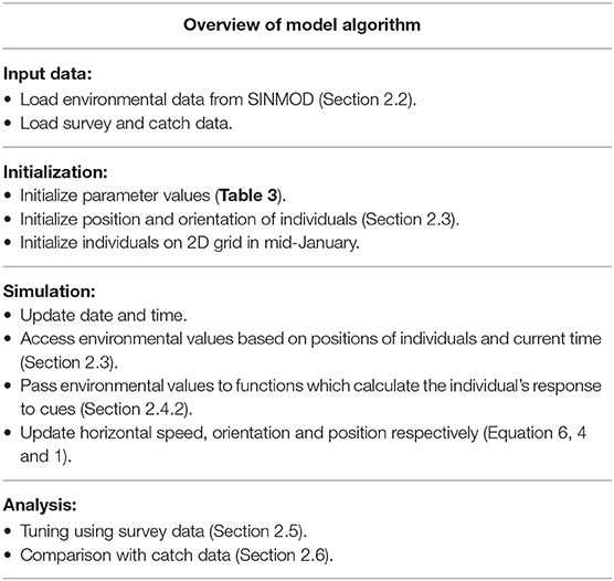
Table 1. Overview of the main components of the model algorithm with reference to associated sections and equations.
Estimates of environmental conditions were loaded from SINMOD, a physical oceanographic model that is based on the primitive Navier–Stokes equations, and uses a z-coordinate grid (Slagstad and McClimans, 2005). The configuration used has 970 × 635 horizontal grid cells with 4km resolution and centres on the Norwegian Sea. The model is divided into 34 vertical depth layers. The IBM developed in this paper modelled individuals in a 2D environment where position was updated on a continuous horizontal plane in a Lagrangian approach (Figure 1). Environmental variables were calculated based on assumptions of the herring's depth preferences, described in section 2.4.1. State variables were updated at discrete time steps of Δt = 4h. Temperatures and current speeds were extracted from SINMOD output from 2015 to 2020, and along with the bathymetry field of the model area, drove changes in fish movements.
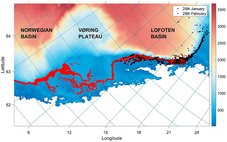
Figure 1. The continuous model system with individuals plotted at two time stamps in the same simulation scenario. The colourmap and colourbar display the bottom depth of grid cell j in metres, while the lines of latitude and longitude extend from ticks along the y and x axes, respectively. The map displays the Norwegian coast and Norwegian Sea from 62 to 72 degrees north, including bathymetry features important in ocean circulation.
The model was developed in MATLAB, which is a matrix-based programming language that is suited for iterative analysis involving numerous matrix operations. Below, the development of the model is outlined in regards to the model system, the main equations, parameters and state variables. Thereafter, we explore tuning and comparison against observations of the real system.
When referring to vectors that can take on continuous values, x and y indices will be used, while the index j will indicate the discrete linear index of a grid cell, ranging from 1 to the number of elements in the grid. Finally, boldface characters denote vectors.
The individual state variables used were position p, orientation angle θ, horizontal speed rb, and horizontal speed offset ro. Position was updated at each discrete time k, with time step Δt:
where:
where p is a vector with the x and y coordinates of the individual in the continuous space of the model grid and vb is a vector with the horizontal velocity components of an individual fish in the x and y directions, based on behavioural cues. Similarly, vc is a vector with the horizontal current velocity components in the x and y directions. The superscript T denotes the transpose of the vector. The spawning migration proceeds counter to the NCC (Slotte and Fiksen, 2000). This is modelled by the term −Φvc that adds a counter-current component to the horizontal speed controlled by the parameter Φ. An individual's realized swimming velocity vf is composed of the counter current term and behavioural responses from vb. This formulation demands individuals respond to the prevailing current with higher priority, relative to other cues. To prevent unrealistic dynamics in the first-order approximation of velocity (vf + vc), the short Δt of 4h was used. The vector vb was calculated as:
where rb is the horizontal speed of the individual in m s−1 and θ the orientation angle according to gradient cues. As indicated before, when ||vc|| approaches zero, the individuals approach a speed of rb with the orientation angle θ. The angle θ was updated as follows:
where α is a weighting parameter, and G is the angle of the vector inputs calculated from near-field gradients, as explored in section 2.4.2. It is likely NSSH base their movements on comparison of conditions from previous experience and present information when calculating their new orientation (Fernö et al., 1998). To account for this, α acted as a low-pass filter, avoiding erratic changes in θ, similar to a formulation by Føre et al. (2009). Furthermore, rb was calculated as a random process with a deviation ro from the cruising speed:
where was the cruising speed in m s−1 of the individual. The value was calibrated during the tuning procedure in section 2.5. The offset ro was then calculated as a Gauss-Markov process with exponential auto-correlation. This meant ro and rb were correlated with recent values. The offset was included to model randomness in the horizontal speed. It was updated as follows:
from a normal distribution with zero mean, a standard deviation σ in swimming speed and shaping parameter for auto-correlation β.
The spawning migration follows overwintering, a stationary period characterized by slow swimming speeds and low energy use. NSSH mainly spawn in southern regions of coastal Norway before migrating westwards to feed over summer. The spawning migration begins early to mid-January and spawning usually begins in late-February/early-March (Dragesund et al., 1980). Temperature and current data for the period from mid-January to the end of February (2015–2020) were loaded from SINMOD, along with the bathymetry. Below, the responses that play a role in the spawning migration are outlined.
Depth is an important variable as it influences the temperature and currents that an individual experiences. Environmental values were calculated as a linear combination of values taken from a depth layer in the upper water column (0–75 m) and the lower water column (75–300 m):
where vc is the horizontal current velocity, T is the temperature, l1 and l2 are the vertical indices of layers sampled in the upper and lower water column, respectively, d was the fraction of daylight at the sampled time and latitude (hours of daylight/24). This approximation allows variability in environmental values, rather than use of values from a constant depth layer. The choice of d as a variable reflected the individuals need to spend time in layers that provide light conditions which facilitate the capacity to school and sense local surroundings (Huse and Ona, 1996). The vertical indices l1 and l2 were chosen based on min(||vc||), as herring have the ability to choose depth layers with favourable current speeds (Nøttestad et al., 1996).
Apart from the direct response to current, individuals responded to the temperature and bottom depth gradients at their location. The orientation angle G was calculated as:
where the angles ∠GD and ∠GT are the gradient dependent orientation angles calculated based on the depth and temperature gradients, respectively, and w is the weighting parameter on ∠GD.
Bottom depth: The NSSH spawning migration develops southward alongside the continental slope (Slotte and Fiksen, 2000). Herring are physostomous with an open swim bladder, which facilitates more rapid vertical movements (Blaxter, 1985; Nøttestad, 1998). Vertical escape is considered central in predator avoidance (Langård et al., 2014). For these reasons, GD was used to direct individuals movements perpendicular to the direction of the depth gradient, in the southerly direction:
where ∇D is the bottom depth gradient and D is the bottom depth at grid point j. The first case reorients individuals toward the coast, while the second case directs individuals southwards along isobaths. The y component of ∇D is multiplied by sign(y) prior to the calculation in the second case.
Temperature: NSSH avoid low temperatures and higher temperatures are associated with superior body condition (Fernö et al., 1998). Therefore, individuals oriented toward higher temperatures, based on the local gradient. If temperatures reached an upper limit, the herring reoriented toward cooler waters based on the near field gradient. The function was formulated as below:
where ∇T is the temperature gradient calculated from the T field in Equation (8).
To develop the individuals responses to environmental information, the parameters [Φ α w]T in Equations (2), (4), and (9) were tuned and then analysed. Simulations with 2017–2020 environmental values and 4 separate initialization scenarios were investigated. In order to model reasonable responses of individuals to their environment the model was tuned using a numerical optimization algorithm that took parameter values as input and minimized the deviation between the model and observed distributions at specific time stamps. NSSH survey data from the Norwegian Institute of Marine Research was used for this purpose (Salthaug et al., 2020). The survey data combines acoustic and trawl data to estimate abundance in predefined strata areas. To ensure consistency, 2017 and 2018 estimates were used for tuning, when the dates sampled were in the last two weeks of February. 2019 and 2020 data provided an independent data set to validate the optimization.
To allow fine grain comparison on specified dates, the following transformation of strata values was carried out, converting observation estimates into numbers per grid cell j:
• A 12 km2 sliding penalty used acoustic zero values to penalize areas sampled with low abundances. This meant that grid cells with strata values in close proximity to those with zero acoustic values were set to zero.
• A 20 km2 sliding mean was then calculated to smooth out areas and maintain spatial patterns of densities.
• The weighted sum of trawl data was used to centre the comparison for single days from the survey. A 52 km2 grid was drawn around the centre as a bin for comparison.
• The transformed observation values were then normalized and scaled according to the number of model individuals (Figure 2).
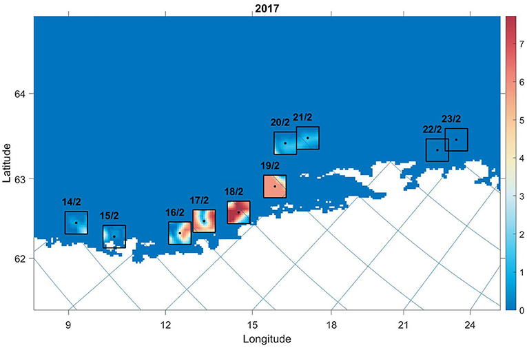
Figure 2. Transformed survey values used to compare against model values on specified dates in 2017. Black dots indicate the weighted sum of trawl values on the date transcribed above the box. The black lines demarcate the outer boundary of cells included for the comparison. The colourmap indicates estimated number of individuals in grid cell j.
This procedure offered individuals specific objective functions for a set of time stamps on the migration path. Thus, an optimization routine was used to find the minimum f in Equation (12). This algorithm tuned the parameters [Φ α w]T and constrained them to between 0 and 1. The densities of individuals were compared with the fraction of modelled individuals at the sampled date as follows:
where i is the year, y is the number of years, N is the number of cells, and xj and are the number of observation and model individuals in grid cell j, respectively. For simplicity, indices indicating day are omitted, where the Root Mean Square Deviation (RMSD) calculation (in parentheses) is executed on the relevant date (Figure 2).
One source of uncertainty is the intialization of the spawning migration. Given we can perform temporal comparisons above, 4 scenarios with different initial locations were selected, based on information from the NSSH survey and the Norwegian Directorate of Fisheries. They represented scenarios where the central mass of individuals were at variable distances from the coast and variable distances north (Table 2). This design tested the sensitivity of the migration to initial conditions. The probability of an individuals presence in grid cell j (pj) was calculated from a gaussian radial basis function with the following equation:
where cj are floored x and y coordinates of grid cell j, Ĉ is the floored centre point x and y coordinates, and ρ is a parameter that controls the spread around Ĉ, which was calibrated in conjunction with the optimization routine. This strategy allowed the fine grain control of initial distribution by proving spatial correlations in p based on distance from Ĉ. These simulations aimed not to fully describe the distribution prior to migration, but provided insights into how such variation can influence model output.
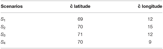
Table 2. Centre points for each scenario.
Normalized RMSD values between transformed survey values and model output was used to gauge the sensitivity of parameters across to initialization scenarios S1 to S4. The parameter values from one scenario was then selected for the remainder of the comparisons. The 2015–2020 SINMOD environmental values were coupled with the IBM to produce 6 distinct realizations.
To inspect the tuning results at high resolution (section 3.2), densities of individuals were post-processed. The number of individuals in each model grid cell j were summed to calculate density per grid cell. Following, a sliding mean calculation for 20 km2 was used to derive spatial correlations in densities. To visualize the central tendency of the trajectory, the weighted sum of latitude and longitude points of individuals were computed for each day. Thereafter, acoustic density values from the NSSH survey were converted to the relative fraction along all transects for the sampled time. Each grid cell j along the transect was sampled for the number of model individuals. The model and observation values were interpolated within 50 m bins from 0 to 500 m based on the bottom depth in grid cell j. Finally, we calculated the fraction of model and observation values in each depth bin. This calculation can illustrate the spread of model and observation values off-coast. The 16-18th of February 2019 and 2020 were chosen for visual inspection.
The model output was compared with 2015–2020 catch data from Norwegian Fisheries Directorate in 5 day ranges. The catch data used were the x and y starting locations of trawling and associated catch weight in kg. The main purpose of this comparison was to investigate where and when the model deviates from observations and what this reveals about the capacity for the IBM to resemble realistic NSSH distributions. The initial model distribution was fixed in each year to focus on relative comparisons.
Observation and model densities were allocated 5 day windows, where catch and model positions and values were described by their centre of mass. These were described as latitude and longitude centre points. Then, model output was analysed using geospatial comparisons, as described in Woillez et al. (2007). The global index of collocation (GIC) indicates how geographical distinct two ditributions are. It is based on the distance between the centre points and the variance around these centres (inertia). A value of 0 means there is no overlap, whilst a value of 1 implies identical distributions. The average GIC value for each year was used to score the model and observation overlap. In addition, RMSD values indicated the average error for the year. Using GIC and RMSD indices illuminate where the model and observations disagree. It also offers insight into potential limitations of comparing model and observation output.
Of the 4 simulation scenarios run, 3 scenarios produced reasonable migration patterns. S1, S2, and S3 performed relatively well (Supplementary Material). S4 is far from continental slope, which is vital information for orientation and therefore couldn't minimize Equation (12) properly. The average Φ value, produced by the tuning process for the four scenarios, was quite high and displayed higher variability (0.78±0.2) compared to α (0.59±0.08) and w (0.65±0.1). This illustrates the sensitivity of the response to the current in relation to starting point. The relatively high α value also shows the importance of fish retaining knowledge of previous states in the migration. These simulations highlight the centrality of the continental slope as a landmark in the migration and how individuals are likely to utilize it. Further comparisons from 2015 to 2020 were made using the fitted parameter values based on S2 values (Table 3).
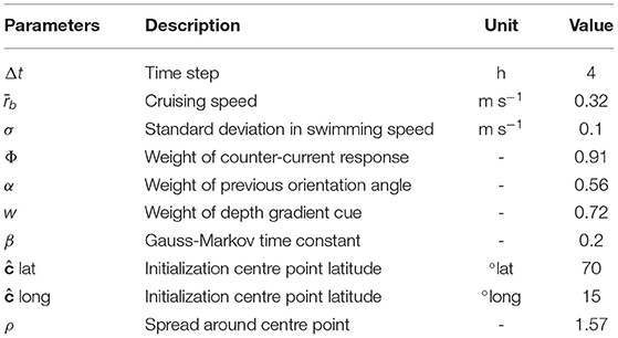
Table 3. Model parameter values.
There was variation in the trajectories of individuals in the migration, especially with regards to longitude (Figure 3). In all cases, the beginning of the migration is quite slow, reflecting the strong current magnitude around the Lofoten basin (Figure 4C). For example, in 2020, the Latitude centre point moves approximately 1 degree from 15/1 - 25/1, in comparison with 1.5 degrees from 9/2 - 19/2. In addition, the longitude centre is more consistent amongst years from 15/1 - 25/1, again reflecting the convergence of environmental cues at this stage, especially ∇D (Figure 4A). There is divergence after this point due to inter-annual variation in T and vc. This demonstrates that environmental variability can produce distinct realizations of the IBM.
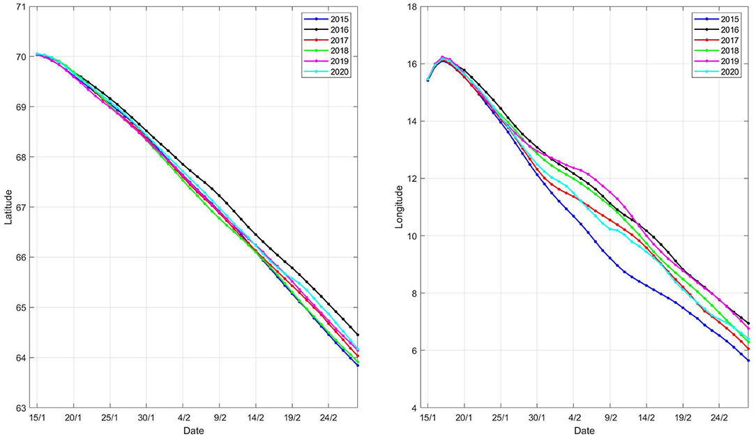
Figure 3. Latitude and longitude centre points during the migration period from S2. Each point was calculated from the weighted sum of individuals per grid cell j.
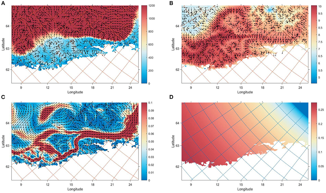
Figure 4. Environmental values that NSSH utilized on the 30th January 2020 relative to their position on the grid. The maps cover the same area as Figure 1: (A) The bottom depth in m (colourmap) and gradient (arrows) (B) The temperature in °C (colourmap) calculated from Equation (8) and gradient (arrows) (C) The x and y components of vc (arrows) calculated from Equation (7). The colourmap shows the magnitude ||vc|| in m s−1 (D) The fraction of daylight d along the Norwegian coast (colourmap), which was used in Equations (7) and (8).
The spatial distribution of individuals illustrates the emergent structures from the simulation (Figure 5). For example, in the 2019 simulation, midway through the migration, emergence of two branches of migration trajectories appeared. One branch extends alongside the continental slope, whilst another curves down toward the coast at approximately 67 degrees latitude and 9 degrees longitude. The 2020 simulation shows similar branching but there is more movement between branches. Toward the end of the migration the individuals push further off-coast, with high densities at 64 degrees latitude and 6 degrees longitude. The two branches join at this point and form a continuous tail that is prominent at the end of February.
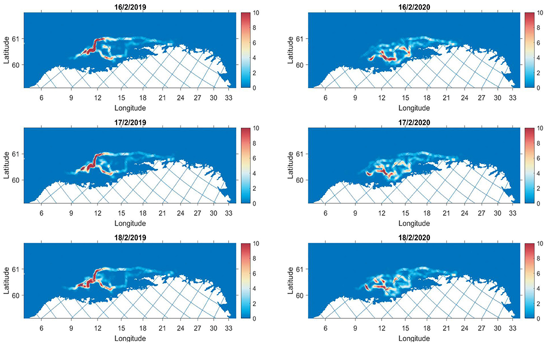
Figure 5. Densities of individuals at 3 time stamps along the migration for 2019 (left column) and 2020 (right column). The colourmap shows the number of individuals in grid cell j.
The high resolution comparison of densities of individuals along acoustic transects with acoustic estimates was useful. It revealed that the model predicts a high spread off coast, not bunching individuals at one particular location (Figure 6). Due to the design of the model, densities are high before tailing off at deep bathymetry (D ≥ 400m), a pattern present in the acoustic data also.
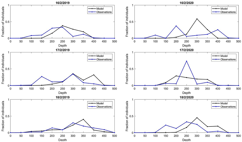
Figure 6. Fraction of estimated model and observation values along acoustic transects at 3 time stamps in 2019 (left column) and 2020 (right column), with associated bottom depth.
In 2/3 of the years there is good agreement between model and catch values (2016, 2017, 2019, and 2020). However, there is intra- and inter-annual variation that can be the result of changes in both fish and vessel behaviour. Below, two simulations are presented with poorer and better agreement between model and observations, respectively (Figures 7, 8).
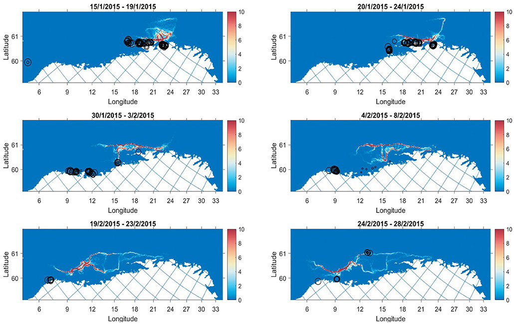
Figure 7. Model output (colourmap) with catch points (black circles) overlayed for selected periods in 2015. Size of circle is scaled to the catch weight. The colourmap gives the average number of individuals in grid cell j for a 5 day period.
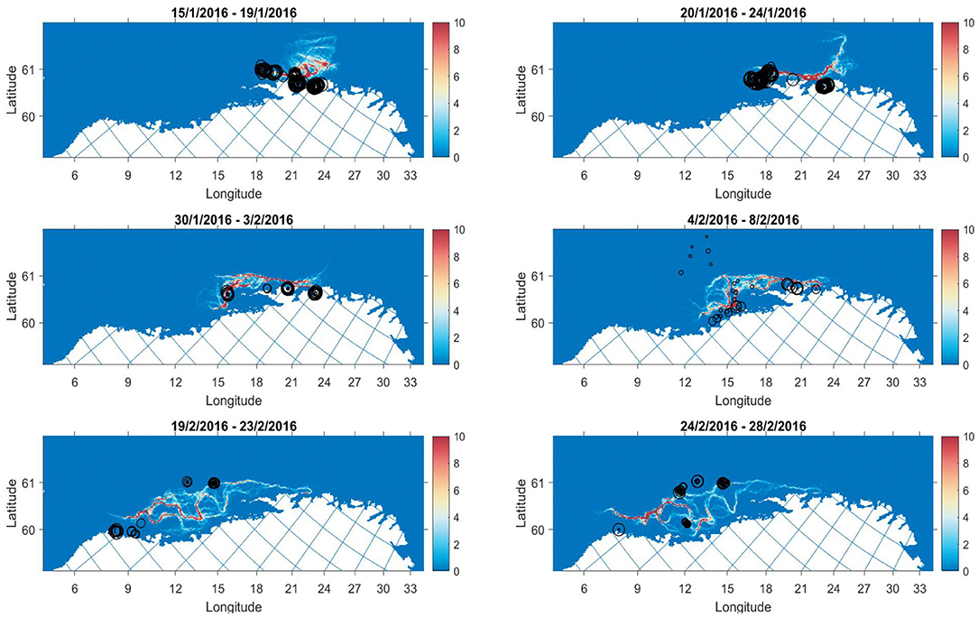
Figure 8. Model output (colourmap) with catch points (black circles) overlayed for selected periods in 2016. Size of circles are scaled according to the catch weight in kg. The colourmap gives the average number of individuals in grid cell j for a 5 day period.
In 2015, the model migration proceeds southerly in a manner that appears slower than the development of catch during this period, particularly from the end of January to the beginning of February, where there are catches in traditional spawning areas at a very early stage of the migration (Figure 7). Survey estimates of abundance from this year were uncertain, where a shift in strong NSSH year classes and immigration from off-coast areas in early February listed as possible explanations for discrepancies (Slotte et al., 2015). Given the comparisons here, it seems there is immigration from off-coast regions.
In contrast, the 2016 catches take place along branches of the migration where the model predicts higher densities (Figure 8). The development of catches overlap with the model evolution. Survey distribution also corroborate findings in early February with observations of high densities around 66–67 degrees latitude (Slotte et al., 2016). The figures from 2017 to 2020 are included in the Supplementary Material.
The centre points for fishing activity is in the northern fjords in mid-January, and the simulations were designed around these starting points. The longitude varies more in this period, suggesting that that the variability is mainly off-coast. In 2018, there was an high off-coast component of catches at the beginning of the season. The least overlap (GIC) and the largest error (RMSD) in location comes from this time (Figures 9, 10). Toward the end of the 2018 season many catches shift to northern regions. The simulation in 2015 deviated from catches also, for reasons which are described in the previous section.
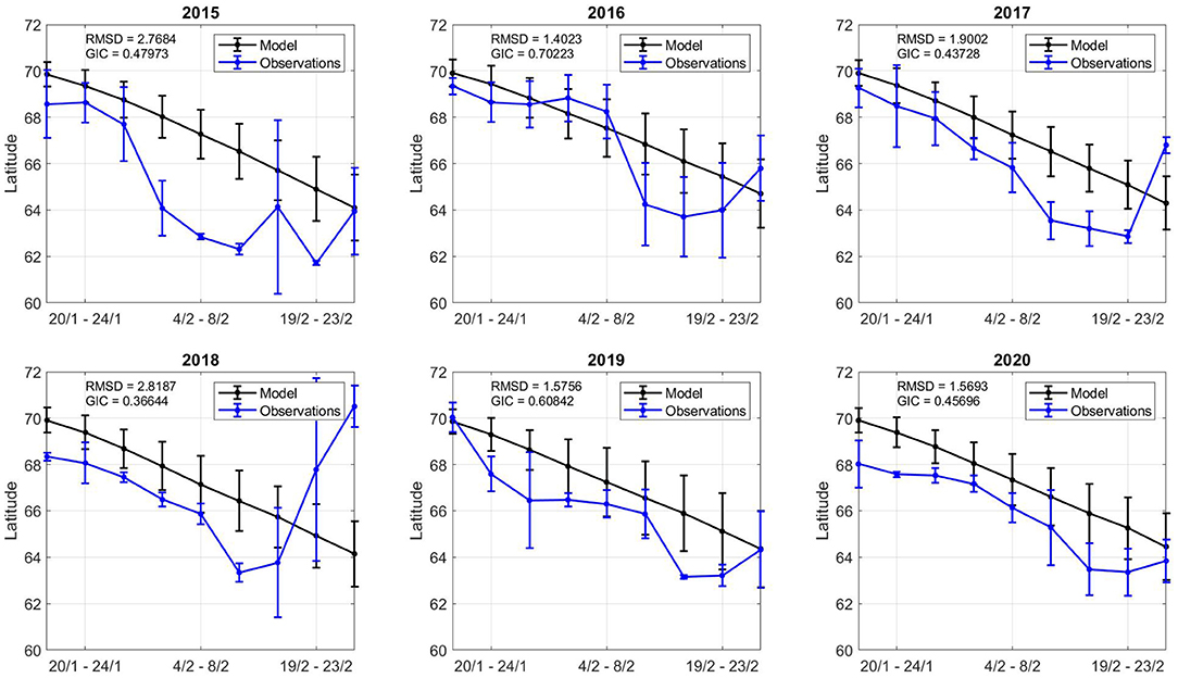
Figure 9. Model and observation comparison across all years. The x axis displays the time period (inclusive). The y axis displays the latitude centre point for catch and model values in the time period. The error bar shows the square root of the inertia values in each time interval.
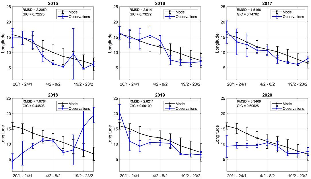
Figure 10. Model and observation comparison across all years. The x axis displays the time period (inclusive). The y axis displays the longitude centre point for catch and model values in the time period. The error bar shows the square root of the inertia values in each time interval.
In general, early February showed the highest GIC values, with lowest RMSD values, suggesting the model dynamics in this period provide reliable geospatial estimates. Both the model and observations shift southward during the simulation time frame. The southern evolution of the catch and the model relate to how NSSH migrates. The spatial variation in centre points (inertia) varies more in observations than model estimates. There are many time periods where there appear catch points spread in space (19/2-23/2 2018) and others when catches are concentrated in one area (4/2-8/2 2018). As the model is physics-based, it has a more constant spatial distribution (inertia and centre points), although there are local differences (Figures 7, 8).
In general, the model showed good agreement with survey and catch observations (Figures 9, 10). Emergent properties of the migration trajectory overlap with vessel catch data. Regardless, there are limitations to modelling behaviour at such low resolutions. There are many sources of uncertainty not fully resolved in this model. Therefore, in conjunction with discussion about the simulations in this paper, we shall detail how models can be improved in future work to improve estimates.
The model formulation required many steps of refinement to give reasonable output. In Equations (1) and (2), the response of the individual was formulated to account for the physical response directly against the prevailing current. Removing the counter-current response led to passive drifting northwards. Running simulations with environmental variables sampled close to the surface resulted in similar drifting patterns, as the magnitude of vc is very high close to the surface, especially around the Lofoten basin (Figure 4C). A formulation that incorporated vertical conditions was important to model, as in Equations (7) and (8).
It is difficult to decouple the low resolution effects of local environmental values on model states, as they are spatially correlated in the horizontal plane. However, the combined effect of reacting to gradients from deep bathymetry, and current patterns seemed the most consistent properties amongst simulations (Figure 4). This study shows that memory- and gradient based reactive mechanisms can be used to model the migration of pelagic fish species such as NSSH (Fernö et al., 1998).
The energetic states of individuals were not included in this study, but may provide more insight into variations in observed patterns. Further work in this project aims to incorporate Dynamic Energy Budget theory, that can be used to model energetic costs of migration (Kooijman, 2000). Thus, state-dependent selection of spawning grounds can be explored, testing the effect of body length and condition on choice of area (Slotte and Fiksen, 2000). Natural mortality may also be included here. Interactions between individuals was explored, such as attraction and repulsion, but deemed difficult to model at the 4 km2 scale. There may be a case to model interactions between schools, where information transfer could potentially give access to novel information, but this is beyond the scope of the project at this stage.
It should be mentioned that the ocean models that force the behaviour of the IBM are subject to their own limitations. Ocean model outputs have uncertainty caused by limits in model resolution, our knowledge of the processes resolved by the model, uncertainty in initial values, boundary conditions, parameter values, and inaccuracies in numerical implementations (Lermusiaux et al., 2006). Additionally, climatic fluctuations can play an important role in survival of recruits and thus, biomass estimates (Toresen and Østvedt, 2000). Therefore, understanding how variability in climate can manifest as variability in individual state and parameter values is important moving forward.
The initialization procedure presented above functioned to generate a generic distribution that was applied to all model scenarios. This provided a realistic initial distribution as input for the tuning procedure. In reality, there is much uncertainty around the initial distribution of NSSH. This may be explained by changes in winter stay areas, which has historic precedent (Dragesund, 1970). Thus, in future work, we shall model initial distributions based on prescient knowledge of winter stay areas and recent catch observations preceding the model run.
Tuning the migration model against survey data allowed for high resolution, time-sensitive estimates of fish densities. There was good agreement between tuned models and independent datasets. Nevertheless, developing the means to calibrate the model was challenging. One difficulty was the progression of the migration in comparison to surveys. The survey starts in southern Norway and progresses northward, the inverse of the NSSH migration. This meant estimates at the beginning and end of survey largely consisted of acoustic absence. In the course of this work, many objective functions for tuning of different resolutions were provided for the individuals and there is room for further experimentation here.
The model was trained using data that has its own biases (e.g., gear selectivity) which may bias the model tuning as a result. Additionally, fisheries data is sparse in space and time. Immigration and recruitment will also sporadically alter fish abundance. As such, one model realization cannot encapsulate the full variation in fish distributions. Adding noise terms to model parameters can be used to produce an ensemble of estimates through Monte Carlo experiments. State and parameter estimates can be obtained effectively in this way (Ward et al., 2016).
The catch data served to judge the performance of the model across the time frame and highlight discrepancies. This shows what the model can and cannot resolve, and at what scales. The physics- based model used assumptions of responses to the prevailing current and gradients to reproduce the likely migration at large-scale. In contrast, catch data reflects which locations were targeted based on market value, quotas, weather conditions, etc. This is variability the model cannot capture. The model output is useful in predicting relevant catch locations in space and time at low resolutions (Figures 9, 10). It gives insight into where the development of model densities is matched with fishing activity and where it does not. The output will have operational use when it is combined with real-time fisheries-dependent data, as described below. The novel use of real-time observations can give time-sensitive estimates that are more reliable than use of model or observation values in isolation.
In future, information on vessel activity will be incorporated to improve observation quality. Classifying vessels in terms of search vs. fishing activity can provide fine-grain, continuous information on the behaviour of fishermen. Thus, one can improve coverage of observations and incorporate absence data. Finally, using a data assimilation procedure, we can improve estimates by combining a model, such as the one developed here, with observation data. Such estimates require expansion of the model to include uncertainties in initial conditions, environmental variables, parameters, etc. We have developed one realization of the model here, but modelling such uncertainties produces multiple realizations, from which one can calculate the most probable estimate of the model state (Evensen, 2009).
Publicly available datasets were analyzed in this study. This data can be found at: https://www.fiskeridir.no/Tall-og-analyse/AApne-data/AApne-datasett/elektronisk-rapportering-ers.
CK: wrote the manuscript, developed the model, processed data, ran the simulations, and produced figures. FM: helped with accessing and processing data, feedback on written work and simulations. JK: input on herring research, feedback on written work. MA: helped with conception of the project, aided with setting up the model, gave constant feedback and suggestions on every aspect of the project. All authors contributed to the article and approved the submitted version.
The work is part of the FishGuider project, which was funded by the project participants and the Norwegian Research Council (Project Number 296321). North Atlantic Institute of Sustainable Fishing (NAIS) is an industry partner that funds 50% of this project.
The authors declare that the research was conducted in the absence of any commercial or financial relationships that could be construed as a potential conflict of interest.
All claims expressed in this article are solely those of the authors and do not necessarily represent those of their affiliated organizations, or those of the publisher, the editors and the reviewers. Any product that may be evaluated in this article, or claim that may be made by its manufacturer, is not guaranteed or endorsed by the publisher.
We greatly acknowledge the support, input and feedback from the project participants: NTNU, SINTEF, NAIS, and UiB. We also acknowledge useful input from discussions with Øystein Varpe at UiB.
The Supplementary Material for this article can be found online at: https://www.frontiersin.org/articles/10.3389/fmars.2021.754476/full#supplementary-material
Alver, M. O., Broch, O. J., Melle, W., Bagøien, E., and Slagstad, D. (2016). Validation of an Eulerian population model for the marine copepod Calanus finmarchicus in the Norwegian Sea. J. Mar. Syst. 160, 81–93. doi: 10.1016/j.jmarsys.2016.04.004
Arnason, R., Magnusson, G., and Agnarsson, S. (2000). The Norwegian spring-spawning herring fishery: a stylized game model. Mar. Resour. Econ. 15, 293–319. doi: 10.1086/mre.15.4.42629328
Baker, R. E., Peña, J.-M., Jayamohan, J., and Jérusalem, A. (2018). Mechanistic models versus machine learning, a fight worth fighting for the biological community? Biol. Lett. 14:20170660. doi: 10.1098/rsbl.2017.0660
Barbaro, A., Einarsson, B., Birnir, B., Sigurðsson, S., Valdimarsson, H., Pálsson, O., Sveinbjörnsson, S., and Sigurðsson, o. (2009). Modelling and simulations of the migration of pelagic fish. ICES J. Mar. Sci. 66, 826–838. doi: 10.1093/icesjms/fsp067
Bauer, S., and Klaassen, M. (2013). Mechanistic models of animal migration behaviour - their diversity, structure and use. J. Anim. Ecol. 82, 498–508. doi: 10.1111/1365-2656.12054
Bjørndal, T., Gordon, D. V., Kaitala, V., and Lindroos, M. (2004). international management strategies for a straddling fish stock: a bio-economic simulation model of the Norwegian spring-spawning herring fishery. Environ. Resour. Econ. 29, 435–457. doi: 10.1007/s10640-004-1045-y
Blaxter, J. H. S. (1985). The herring: a successful species? Can. J. Fish. Aquat. Sci. 42, s21–s30. doi: 10.1139/f85-259
Boyd, R., Sibly, R., Hyder, K., Walker, N., Thorpe, R., and Roy, S. (2020). Simulating the summer feeding distribution of Northeast Atlantic mackerel with a mechanistic individual-based model. Progr. Oceanogr. 183:102299. doi: 10.1016/j.pocean.2020.102299
Chu, D. (2011). Technology evolution and advances in fisheries acoustICS. J. Mar. Sci. Technol. 19:2. doi: 10.51400/2709-6998.2188
Dragesund, O. (1970). Factors influencing year-class strength of norwegian spring spawning herring (clupea harengus l.). Fiskeridirektoratets Skrifter Serie Havundersøkelser 15, 381–450.
Dragesund, O., Hamre, J., and Øyvind, U. (1980). Biology and population dynamics of the Norwegian spring- spawning herring. Rapports et Procès-Verbaux des Rèunions 177, 43–71.
Fernö, A., Pitcher, T. J., Melle, W., Nøttestad, L., Mackinson, S., Hollingworth, C., et al. (1998). The challenge of the herring in the Norwegian sea: making optimal collective spatial decisions. Sarsia 83, 149–167. doi: 10.1080/00364827.1998.10413679
Fiksen, Ø., and Slotte, A. (2002). Stock environment recruitment models for norwegian spring spawning herring (clupea harengus). Can. J. Fish. Aquat. Sci. 59, 211–217. doi: 10.1139/f02-002
Føre, M., Dempster, T., Alfredsen, J. A., Johansen, V., and Johansson, D. (2009). Modelling of Atlantic salmon (Salmo salar L.) behaviour in sea-cages: a Lagrangian approach. Aquaculture 288, 196–204. doi: 10.1016/j.aquaculture.2008.11.031
Giske, J., Huse, G., and Berntsen, J. (2001). Spatial modelling for marine resource management, with a focus on fish. Sarsia 86, 405–410. doi: 10.1080/00364827.2001.10420482
Grimm, V., Berger, U., Bastiansen, F., Eliassen, S., Ginot, V., Giske, J., et al. (2006). A standard protocol for describing individual-based and agent-based models. Ecol. Model. 198, 115–126. doi: 10.1016/j.ecolmodel.2006.04.023
Grimm, V., and Railsback, S. F. (2005). Individual-Based Modeling and Ecology. Princeton: Princeton University Press, 3–21.
Huse, I., and Ona, E. (1996). Tilt angle distribution and swimming speed of overwintering Norwegian spring spawning herring. ICES J. Mar. Sci. 53, 863–873. doi: 10.1006/jmsc.1996.9999
Kooijman, S. A. L. M. (2000). Dynamic Energy and Mass Budgets in Biological Systems, 2 Edn. Cambridge: Cambridge University Press.
Langård, L., Fatnes, O., Johannessen, A., Skaret, G., Axelsen, B., Nöttestad, L., et al. (2014). State-dependent spatial and intra-school dynamics in pre-spawning herring Clupea harengus in a semi-enclosed ecosystem. Mar. Ecol. Progr. Ser. 501, 251–263. doi: 10.3354/meps10718
Lermusiaux, P. F., Chiu, C., Gawarkiewicz, G., Abbot, P., Robinson, A., Miller, R. N., et al. (2006). Quantifying uncertainties in ocean predictions. Oceanography 19, 90–103. doi: 10.5670/oceanog.2006.93
Nøttestad, L. (1998). Extensive gas bubble release in Norwegian spring-spawning herring (Clupea harengus) during predator avoidance. ICES J. Mar. Sci. 55, 1133–1140. doi: 10.1006/jmsc.1998.0416
Nøttestad, L., Aksland, M., Beltestad, A., Fernö, A., Johannessen, A., and Arve Misund, O. (1996). Schooling dynamics of norwegian spring spawning herring (Clupea harengus L.) in a coastal spawning area. Sarsia 80, 277–284. doi: 10.1080/00364827.1996.10413601
Pennino, M. G., Conesa, D., López-Quílez, A., Muñoz, F., Fernández, A., and Bellido, J. M. (2016). Fishery-dependent and -independent data lead to consistent estimations of essential habitats. ICES J. Mar. Sci. 73, 2302–2310. doi: 10.1093/icesjms/fsw062
Politikos, D., Somarakis, S., Tsiaras, K., Giannoulaki, M., Petihakis, G., Machias, A., and Triantafyllou, G. (2015). Simulating anchovy's full life cycle in the northern Aegean Sea (eastern Mediterranean): a coupled hydro-biogeochemical–IBM model. Progr. Oceanogr. 138, 399–416. doi: 10.1016/j.pocean.2014.09.002
Salthaug, A., Stenevik, E., Vatnehol, S., Anthonypillai, V., Ona, E., Anthonypillai, V., et al. (2020). Distribution and Abundance of Norwegian Spring Spawning Herring During the Spawning Season in 2020. Technical Report, Institute of Marine Research, Bergen, Norway.
Slagstad, D., and McClimans, T. A. (2005). Modeling the ecosystem dynamics of the barents sea including the marginal ice zone: i. physical and chemical oceanography. J. Mar. Syst. 58, 1–18. doi: 10.1016/j.jmarsys.2005.05.005
Slotte, A., and Fiksen, Ø. (2000). State-dependent spawning migration in Norwegian spring-spawning herring. J. Fish Biol. 56, 138–162. doi: 10.1111/J.1095-8649.2000.TB02091.X
Slotte, A., Johnsen, E., Pena, H., Salthaug, A., Utne, K., Anthonypillai, V., et al. (2015). Distribution and Abundance of Norwegian Spring Spawning Herring During the Spawning Season in 2015. Technical Report, Institute of Marine Research, Bergen, Norway.
Slotte, A., Salthaug, A., Utne, K., Ona, E., Vatnehol, S., and Pena, H. (2016). Distribution and Abundance of Norwegian Spring Spawning Herring During the Spawning Season in 2016. Technical Report, Institute of Marine Research, Bergen, Norway.
Tamario, C., Sunde, J., Petersson, E., Tibblin, P., and Forsman, A. (2019). Ecological and evolutionary consequences of environmental change and management actions for migrating fish. Front. Ecol. Evol. 7:271. doi: 10.3389/fevo.2019.00271
Toresen, R., and Østvedt, O. (2000). Variation in abundance of norwegian spring-spawning herring (clupea harengus, clupeidae) throughout the 20th century and the influence of climatic fluctuations. Fish Fisheries 1, 231–256. doi: 10.1111/j.1467-2979.2000.00022.x
Touzeau, S., Lindroos, M., Kaitala, V., and Ylikarjula, J. (2000). Economic and biological risk analysis of the norwegian spring-spawning herring fishery. Ann. Oper. Res. 94, 197–217. doi: 10.1023/A:1018973217951
Tu, C.-Y., Tseng, Y.-H., Chiu, T.-S., Shen, M.-L., and Hsieh, C.-H. (2012). Using coupled fish behavior-hydrodynamic model to investigate spawning migration of Japanese anchovy, Engraulis japonicus, from the East China Sea to Taiwan: Spawning migration model of Japanese anchovy. Fish. Oceanogr. 21, 255–268. doi: 10.1111/j.1365-2419.2012.00619.x
Varpe, Ø., Fiksen, Ø., and Slotte, A. (2005). Meta-ecosystems and biological energy transport from ocean to coast: the ecological importance of herring migration. Oecologia 146, 443. doi: 10.1007/s00442-005-0219-9
Ward, J. A., Evans, A. J., and Malleson, N. S. (2016). Dynamic calibration of agent-based models using data assimilation. R. Soc. Open Sci. 3, 150703. doi: 10.1098/rsos.150703
Keywords: individual, model, migration, observation, catch, tuning, comparison, spawning
Citation: Kelly C, Michelsen FA, Kolding J and Alver MO (2022) Tuning and Development of an Individual-Based Model of the Herring Spawning Migration. Front. Mar. Sci. 8:754476. doi: 10.3389/fmars.2021.754476
Received: 06 August 2021; Accepted: 15 December 2021;
Published: 13 January 2022.
Edited by:
Jie Cao, North Carolina State University, United StatesReviewed by:
Chongliang Zhang, Ocean University of China, ChinaCopyright © 2022 Kelly, Michelsen, Kolding and Alver. This is an open-access article distributed under the terms of the Creative Commons Attribution License (CC BY). The use, distribution or reproduction in other forums is permitted, provided the original author(s) and the copyright owner(s) are credited and that the original publication in this journal is cited, in accordance with accepted academic practice. No use, distribution or reproduction is permitted which does not comply with these terms.
*Correspondence: Cian Kelly, Y2lhbi5rZWxseUBudG51Lm5v
Disclaimer: All claims expressed in this article are solely those of the authors and do not necessarily represent those of their affiliated organizations, or those of the publisher, the editors and the reviewers. Any product that may be evaluated in this article or claim that may be made by its manufacturer is not guaranteed or endorsed by the publisher.
Research integrity at Frontiers
Learn more about the work of our research integrity team to safeguard the quality of each article we publish.