 Karlina Merkens1*
 Simone Baumann-Pickering2
 Morgan A. Ziegenhorn2
 Jennifer S. Trickey2
 Ann N. Allen3
 Erin M. Oleson3
- 1Saltwater Inc., Portland, OR, United States
- 2Scripps Institution of Oceanography, University of California, San Diego, La Jolla, CA, United States
- 3NOAA Fisheries Pacific Islands Fisheries Science Center, Honolulu, HI, United States
Many animals use sound for communication, navigation, and foraging, particularly in deep water or at night when light is limited, so describing the soundscape is essential for understanding, protecting, and managing these species and their environments. The nearshore deep-water acoustic environment off the coast of Kona, Hawai’i, is not well documented but is expected to be strongly influenced by anthropogenic activities such as fishing, tourism, and other vessel activity. To characterize the deep-water soundscape in this area we used High-frequency Acoustic Recording Packages (HARPs) to record acoustic data year-round at a 200 or 320 kHz sampling rate. We analyzed data spanning more than 10 years (2007-2018) by producing measurements of frequency-specific energy and using a suite of detectors and classifiers for general and specific sound sources. This provided a time series for sounds coming from biological, anthropogenic and physical sources. The soundscape in this location is dominated by signals generated by humans and odontocete cetaceans (mostly delphinids), generally alternating on a diel cycle. During daylight hours the dominant sound sources are vessels and echosounders, with strong signals ranging from 10 Hz to 80 kHz and above, while during the night the clicks from odontocetes dominate the soundscape in mid-to-high frequencies, generally between 10 and 90 kHz. Winter-resident humpback whales are present seasonally and produce calls in lower frequencies (200-2,000 Hz). Overall, seasonal variability is relatively subtle, which is unsurprising given the tropical latitude and deep-water environment. These results, and particularly the inclusion of sounds from frequencies above 2 kHz, represent the first long-term analysis of a marine soundscape in the North Pacific, and the first assessment of the intense, daily presence of manmade noise at this site. The decadal time series allows us to characterize the dynamic nature of this location, and to begin to identify changes in the soundscape over time. This type of analysis facilitates protection of natural resources and effective management of human activities in an ecologically important area.
Introduction
Even in the vast, deep ocean a cacophony of sounds may greet the listening ear (or hydrophone). When combined, these sounds form a soundscape, the whole acoustic environment comprising sounds from biological, geophysical and anthropogenic sources (Krause, 2008; Pijanowski et al., 2011). Analysis of the marine soundscape has been used to characterize biodiversity (Bertucci et al., 2016; Harris et al., 2016), indicate ecosystem health (Mathias et al., 2016; Coquereau et al., 2017; Marley et al., 2017), and reveal changes in anthropogenic activity over time (e.g., Andrew et al., 2002; McDonald et al., 2006; Chapman and Price, 2011; McKenna et al., 2012a; Širović et al., 2016). However, most of these studies have been limited in recording depth (most shallower than 50 m), frequency spectrum (many below 2 kHz), and sample duration (e.g., only a few days or months). These limitations prevent analysis over timescales that are biologically relevant to long-lived animals or their communities. Additionally, the frequency range covered by most studies does not span the full frequency range of animal hearing and sound production, particularly in deep-water, open-ocean environments.
As sound is essential for the survival of most marine species, comprehensive understanding of the marine soundscape is important. Marine animals from invertebrates to mammals use sound to forage (e.g., Au, 1993; Chapuis and Bshary, 2010), communicate (e.g., Fine et al., 1977; Staaterman et al., 2010; Janik and Sayigh, 2013; Ladich, 2015), guide settlement (e.g., Mann et al., 2007; Radford et al., 2011; Rice et al., 2017), navigate (e.g., Payne and Webb, 1971; George et al., 1989; Jaquet et al., 2001), and facilitate reproduction (e.g., Popper et al., 2001; Parsons et al., 2008). Regardless of the exact purpose of the sounds that an animal produces or receives, animals experience the soundscape as a holistic environment, and their ability to detect a signal depends on both their sound-detection capabilities as well as the presence of other sounds (e.g., Ketten, 1994; Szymanski et al., 1999; Popper et al., 2001, 2019; Mooney et al., 2010). While natural soundscapes are often made up of a large variety of biophonic and geophonic signals (Hildebrand, 2009; Pijanowski et al., 2011), the introduction of anthropogenic sounds has had a dramatic impact on all acoustic environments, from estuaries (e.g., Marley et al., 2016; Ricci et al., 2016) and shallow coasts and reefs (e.g., Haxel et al., 2013; Bertucci et al., 2016; Cholewiak et al., 2018) to the deep sea (e.g., McDonald et al., 2006; Erbe et al., 2015; Dziak et al., 2017). The presence of anthropogenic sounds in marine soundscapes has been increasing with time and is likely to continue increasing, which has motivated global efforts to monitor marine soundscapes and ocean noise pollution (e.g., Dekeling et al., 2014; Gedamke et al., 2016; Hatch et al., 2016; Haver et al., 2018).
Despite the rapid increase in soundscape research over the last decade (Web of Science search on June 23, 2021 for articles with “soundscape” and “marine” as the topic: years ≤ 2015 = 32, years > 2015 = 193), few attempts have been made to characterize soundscapes in ocean waters below 100-m depth (number of studies: ∼9). Even fewer studies focused on time scales longer than 1 year (number of studies: ∼6). While an increasing number of researchers are collecting data at sampling rates above 2 kHz (e.g., Buscaino et al., 2016; Heenehan et al., 2017; Hermannsen et al., 2019; Magnier and Gervaise, 2020), none have yet been able to monitor these higher frequencies in deep water over long time periods. Given these gaps in understanding, we sought to address the question “what are the characteristics of the soundscape in deep waters across the frequency range of animal hearing over a long time scale?”
To address this question, we used passive acoustic data from instruments moored at ∼650 m depth off the coast of the island of Hawai’i during a 10-year period between 2007 and 2018, with an effective frequency range spanning 10 Hz to either 100 or 160 kHz. The monitoring site was close to shore (∼5 km) in a region with abundant recreational and commercial activity, including deep-sea fishing and offshore fish farming, and other boat-based tourist activities. This site was also located within the United States Navy’s Hawai’i Testing and Training Range and was therefore impacted by national and international military training activities, such as the biannual RIMPAC. Additionally, the site was initially selected with the goal of monitoring the presence of island-associated and/or deep-diving cetacean species, and has been the location of a long-term study of marine mammal occurrence based on visual observations (e.g., Baird et al., 2013). Data from this location has been used in a previous low-frequency (<1 kHz) soundscape study, including a small portion of the data analyzed here (Širović et al., 2016). We relied on a suite of tools including frequency-specific soundscape measurements, manual screening, and automated detectors to identify individual signals, to characterize the sounds from different sources, and to describe their presence over time. Contributions of these individual sound sources to certain frequency bands of interest were quantified to provide information about temporal trends before narrowing in to identify relevant details. The results reveal the complexity of the soundscape and its variability over a variety of temporal scales.
Materials and Methods
Acoustic Data Collection
Passive acoustic data were collected using High-frequency Acoustic Recording Packages (HARPs) (Wiggins and Hildebrand, 2007). Each deployment included a single moored instrument that was located as close as possible to a target location approximately 5 km off the coast of Kona, Hawai’i (Figure 1), with an average depth of 650 m. Some small variations in the exact drop location (10s of m), combined with the steep slope of the island at this site, resulted in some variation of depths (range 460-720 m). The deployments spanned the 2007–2018 time period, with intermittent gaps between deployments due to servicing schedules and/or limits of battery life and data capacity (Table 1).
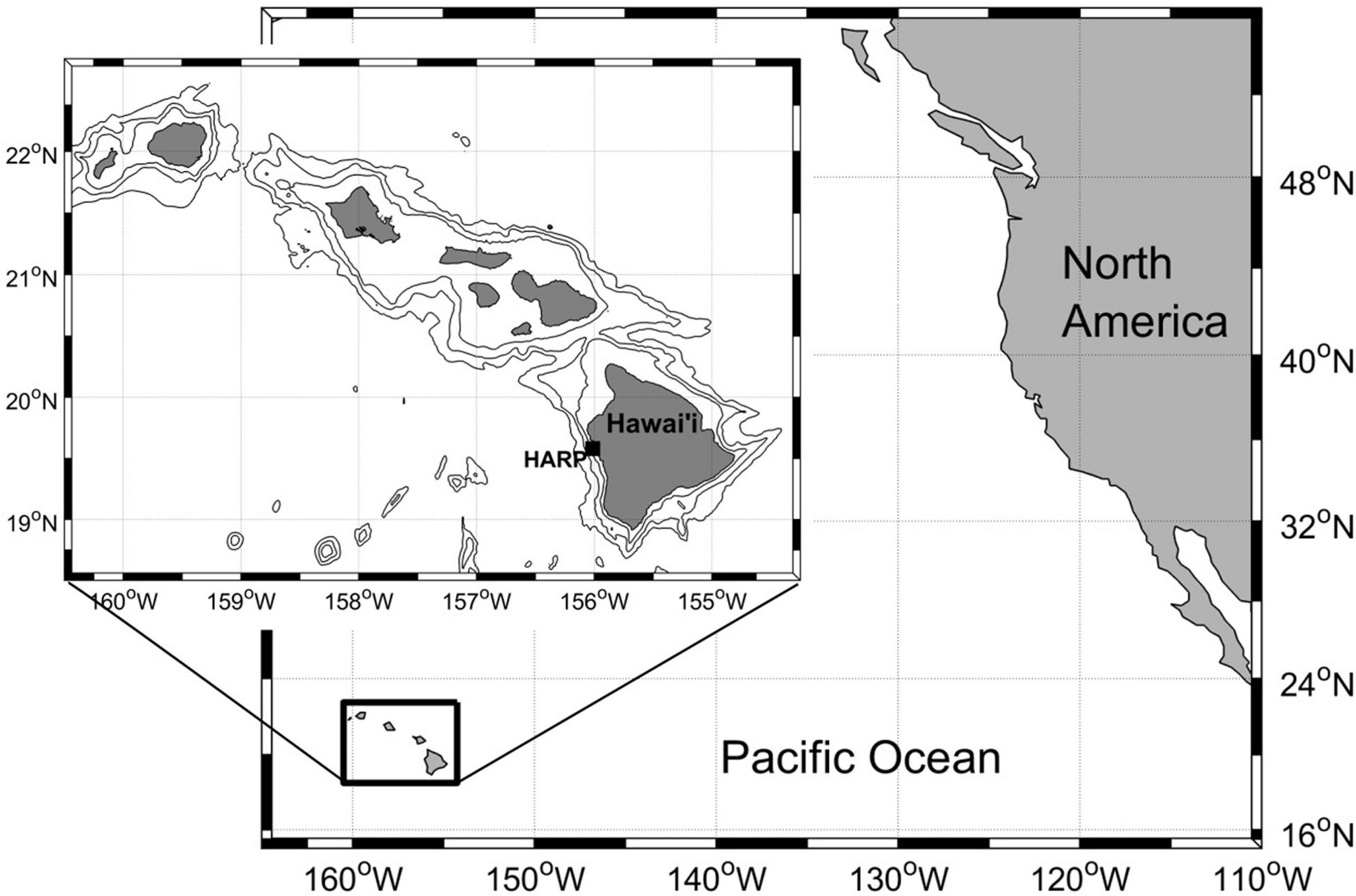
Figure 1. Map of research location, on the western slope of the Big Island of Hawai’i. HARP (black square) was deployed in 600-900 m of water, at approximately 156.0° W and 19.6° N. Bathymetry lines in inset indicate 1,000-m isobaths.

Table 1. Deployment details.
Each instrument included a hydrophone suspended 10–20 m above the sea floor with two stages: a low-frequency stage (10–2,000 Hz or 10–25,000 Hz, Table 1) and a high-frequency stage (2–100 kHz or 25–100 kHz) (Wiggins and Hildebrand, 2007). The sensors were connected to custom-built preamplifier boards with bandpass filters. Each hydrophone was calibrated in the laboratory to provide a quantitative analysis of the received sound field. Representative data loggers and hydrophones were also calibrated at the Navy’s Transducer Evaluation Center facility to verify the laboratory calibrations. Additionally, these calibrations were cross-checked with expected amplitudes given local wind conditions (Hildebrand et al., 2021). Instruments recorded at either a 200 or a 320 kHz sampling rate with 16-bit quantization (Table 1). These sampling frequencies were selected with the goal of spanning the hearing and sound production range of all cetacean species.
Different duty cycle schedules were used to maximize recording duration, with each deployment either having a single, consistent duty-cycle or recording continuously. Within duty-cycled deployments, data were recorded for 5 min, followed by an “off” period ranging from 1 to 20 min. Data gaps, both those between deployments and the “off” periods during duty cycles, forced adjustments for recording effort and prevented us from using standard time series analysis methods that are based on continuous measurements across the full duration of the time series.
Signal Processing and Detection/Classification
Acoustic data were processed in multiple ways to meet the requirements of the detection and classification tools that were selected for the various signal types. All signal processing was performed using the MATLAB-based (Mathworks, Natick, MA, United States) custom software program Triton (Wiggins and Hildebrand, 20071) and other MATLAB custom routines. The appropriate calibration information for each hydrophone and pre-amplifier was applied during analysis of all data products. A suite of soundscape metrics of various bandwidths was calculated, spanning frequencies below 100 Hz to above 50 kHz.
Computation of Soundscape Metrics
Soundscape metrics were computed using the Triton “Remora” (a type of plug-in) Soundscape-Metrics (see text footnote 1). The full time series was split into two frequency bands to allow for more detailed evaluation of the noise components within each frequency band, (A) low-frequency: 10-1,000 Hz and (B) broadband: 100 Hz–100 kHz. Periods of disk-write noise of 15 s, occurring on a repeating cycle every 75 s, were omitted from analysis. Power spectral densities (PSDs) were computed using Welch’s Method within MATLAB. For the low-frequency dataset, acoustic data were low-pass filtered and decimated to a 2,000 Hz sampling rate prior to analysis. Subsequently, a Hanning window was applied and the data were processed to 1 Hz, 1-s resolution (FFT length = 1,000 points, FFT overlap = 0%). Broadband data were also processed using a Hanning window, and the long-term spectral average (LTSA, following Wiggins and Hildebrand, 2007) was calculated with 100 Hz bin width (bw), 1-s resolution (FFT length = 1,000 points, FFT overlap = 0%). The median of mean-square pressure amplitude (μPa2) for each frequency bin was calculated for all hours that contained at least 360 s of data per that hour. The amplitude was then converted to decibels, and, in the case of the broadband data, adjusted for bin width (bw) by subtracting 10 × log10(bw) from each spectral bin, resulting in values of dB re 1 μPa2/Hz.
To facilitate the comparison of soundscape metrics to biological, anthropogenic and abiotic signals, standard frequency bands (American National Standards Institute, ANSI 1.11-2004) were selected and levels were calculated for the following nominal frequencies: 125 Hz, 250 Hz, 500 Hz, 4 kHz, 10 kHz, 20 kHz, 31.5 kHz octaves and 500 Hz third-octave. Additionally, a 1 Hz-wide band spanning 900-901 Hz as well as a 100 Hz-wide band spanning 50.0-50.1 kHz were calculated, with the intention of measuring energy from the specific sound sources described below. The levels in different bands were used to assess temporal trends and were compared to the detection rates for specific signal types to check for correlation between the soundscape metrics and the detected signals.
Detection of Anthropogenic Signals
The occurrence of vessel noise was examined within the full bandwidth data using an automated vessel detector described by Solsona-Berga et al. (2020, Supplementary Material). Briefly, the detector was used on LTSAs computed with 100-Hz frequency bins and 5-s granularity. The detector computed the average power spectral densities (APSD) per 5-s time bin across three LTSA frequency bands, low (1-5 kHz), medium (5-10 kHz), and high (10-50 kHz). Adaptive thresholds were determined over sequential 2-h windows to identify periods of transient signals above ambient noise. When energy in the lower 2 or all 3 frequency bands exceeded specified thresholds for longer than 150 s, the time period over which the thresholds were exceeded was identified as a vessel passage and the start and end times of the passage were recorded. The frequency range of the low, medium, and high bands and the duration of the presence threshold were selected to maximize the number of true positive vessel detections while minimizing the rate of false positives. A random subset of the detections was manually verified and the rate of false positives and missed detections was qualitatively evaluated to ensure satisfactory performance. The detections from this tool are likely an underestimate of vessel presence, particularly during daytime hours, because the dynamic nature of the tool means that 2-h windows with a large amount of continuous vessel energy will have a higher threshold and therefore only extremely high-energy vessel signals will be detected.
Fisheries echosounder pings were identified using a correlation-based detector that compared the normalized waveform envelope of a template echosounder pulse to that of 75- or 43.75-s time series segments (dependent on 200 or 320 kHz sampling frequency, respectively) with signal content between 20 and 80 kHz. In all cases, the waveform envelope was calculated as in Au (1993) and these values were then normalized to scale between 0 and 1. Subsegments within that 75-s segment that had a correlation value above 50% and a separation of >0.05 s were retained and treated as distinct detections, and the timing between successive detections (inter-ping interval) was calculated. Detections with an inter-ping interval outside the range of 0.2-5 s were removed. To further prune out false detections, the mode of the inter-ping interval was calculated and only detections with intervals within 0.1 s of that mode were retained. Counts of echosounder pings per hour were calculated using these retained signals.
Detection of Cetacean Acoustic Signals
Echolocation signals from odontocetes were detected to examine their contribution to the Kona soundscape. Whistles were not examined, though manual review of the data suggests that most periods of delphinid acoustic activity include echolocation clicks, such that nearly all acoustic odontocete presence is represented by focusing on echolocation clicks. Two parallel processes were used to determine the presence of odontocetes in the soundscape.
For the first process, the goal was to calculate a percentage of minutes per hour with odontocete clicks present. Odontocete echolocation clicks (excluding sperm whale clicks, which are too low frequency) were automatically detected using methods described in Roch et al. (2011), with a 10 dB signal-to-noise ratio threshold and signal content between 20 and 90 kHz. Odontocete-positive-minutes per hour were calculated and then divided by recording effort to account for varying duty cycles, resulting in a time series of the percentage of odontocete-positive-minutes per hour.
For the second process the goal was to calculate the average number of clicks per minute in each hour. In this process, echolocation signals were again automatically detected using the same method described above, but with slightly different settings: detecting signals with a peak-to-peak received level above 115 dB and signal content between 10 and 100 kHz. Detections with a peak frequency in echosounder ping-dominated bands (37-39 kHz, 49-51 kHz) were removed to eliminate possible false positives from echosounders. Signals with a peak frequency below 25 kHz were removed to prevent the inclusion of false detections from ships or other low frequency noise sources. Counts of all remaining echolocation clicks per hour were computed. These clicks per hour were then divided by the recording effort in that hour (determined by duty cycle), to produce the average number of clicks per minute in each hour.
Periods of humpback whale (Megaptera novaeangliae) singing were identified using a Convolutional Neural Network trained on this and other HARP data sets (Allen et al., 2021). The recordings were binned into 75-s intervals, and marked as either positive or negative for humpback song presence based on a threshold that gave a precision of 0.97 and recall of 0.93. The minutes per hour with humpback whale presence were calculated and divided by the recording effort in that hour, to determine the percentage of humpback-whale-positive minutes per hour.
Examining Variability in the Soundscape
Diel and Seasonal Trends
Graphs of detections were generated in MATLAB to assess trends over time, including diel and seasonal cycles. Because each deployment spanned many days, and therefore many diel cycles, there was nearly equal effort for all hours of the day within each deployment and across the full data set. Additionally, it was assumed that daily cycles of signal presence did not change seasonally. In contrast, there was a notable difference in effort from season to season, with much lower effort during spring months, particularly March and April, which greatly reduced the power of our analysis to distinguish between real seasonal variation in signal presence and the effect of different amounts of effort. Given this limitation, any seasonal patterns due to springtime increases or decreases were not considered further.
Correlations between the band-level soundscape metrics and the detector-generated, single-source products across the full time series were calculated using the non-parametric Pearson’s linear correlation coefficient, which results in a rho value of 1 or −1 for perfect correlation and 0 when there is no correlation. Additionally, p-values were calculated to indicate the likelihood that the amount of correlation occurred by chance. For the vessel detections, where the duty cycle had a notable impact on the performance of the detector, the correlation was also calculated on a per-deployment basis, to assess the correlation with different duty cycles. For the humpback whale calls, which are intensely seasonal, the correlation was calculated only during the winter season when they are expected to be present.
No-Vessel Periods
Throughout the monitoring period events occurred that temporarily reduced or ceased vessel traffic in the region of the HARP, particularly tsunami and hurricane warnings. These time periods were identified based on a list of regional hurricane events (NOAA National Hurricane Center2) and personal knowledge of other events (e.g., the 2011 Tohoku, Japan Earthquake). For each event, long-term spectral averages were examined to determine whether there were any daytime periods longer than 6 h with no vessel or echosounder activity. Two events were identified for further analysis: the passages of Hurricane Iselle (August 8, 2014) and Hurricane Darby (July 24, 2016) (Table 2). During each of these no-vessel periods, the presence of biological signals was monitored and soundscape metrics were computed. We examined each event by looking at a time period that spanned 2 weeks before the event through 2 weeks following the event, and plotted multiple signal types during that time window, including wind speed measurements from the Kona International Airport, odontocete detections, vessel and echosounder detections and sound energy in different frequency bands. Multiple frequency bands were examined, including the 125 Hz, 250 Hz, 500 Hz, 2 kHz, 4 kHz, 10 kHz and 20 kHz octaves and a 1-Hz band spanning 900–901 Hz. Additionally the mean spectra were plotted for 20-1,500 Hz for data from daytime hours and from nighttime hours during each no-vessel period and during matching hours from 1 week (7 days) prior to each period.
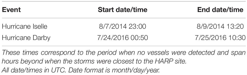
Table 2. Start and end times of the no-vessel periods, and distance to point of closest approach during Hurricanes Iselle and Darby.
Results
Trends in Soundscape Metrics
The entire data set can be viewed as a set of annual long-term spectral averages of each calendar year (Figure 2). This view demonstrates the remarkable extent of the data over time, and also illustrates gaps or changes in monitoring effort (e.g., limited coverage in March throughout all years). The long term and seasonal trends were subtle, with relatively constant soundscape composition across all years and most seasons. The soundscape at lower frequencies (<1,000 Hz) did vary seasonally (Figure 3), with higher levels across all frequencies during winter months (January/February/March). Spring, summer and fall seasons had similar energy across all frequencies in the 10–1,000 Hz range.
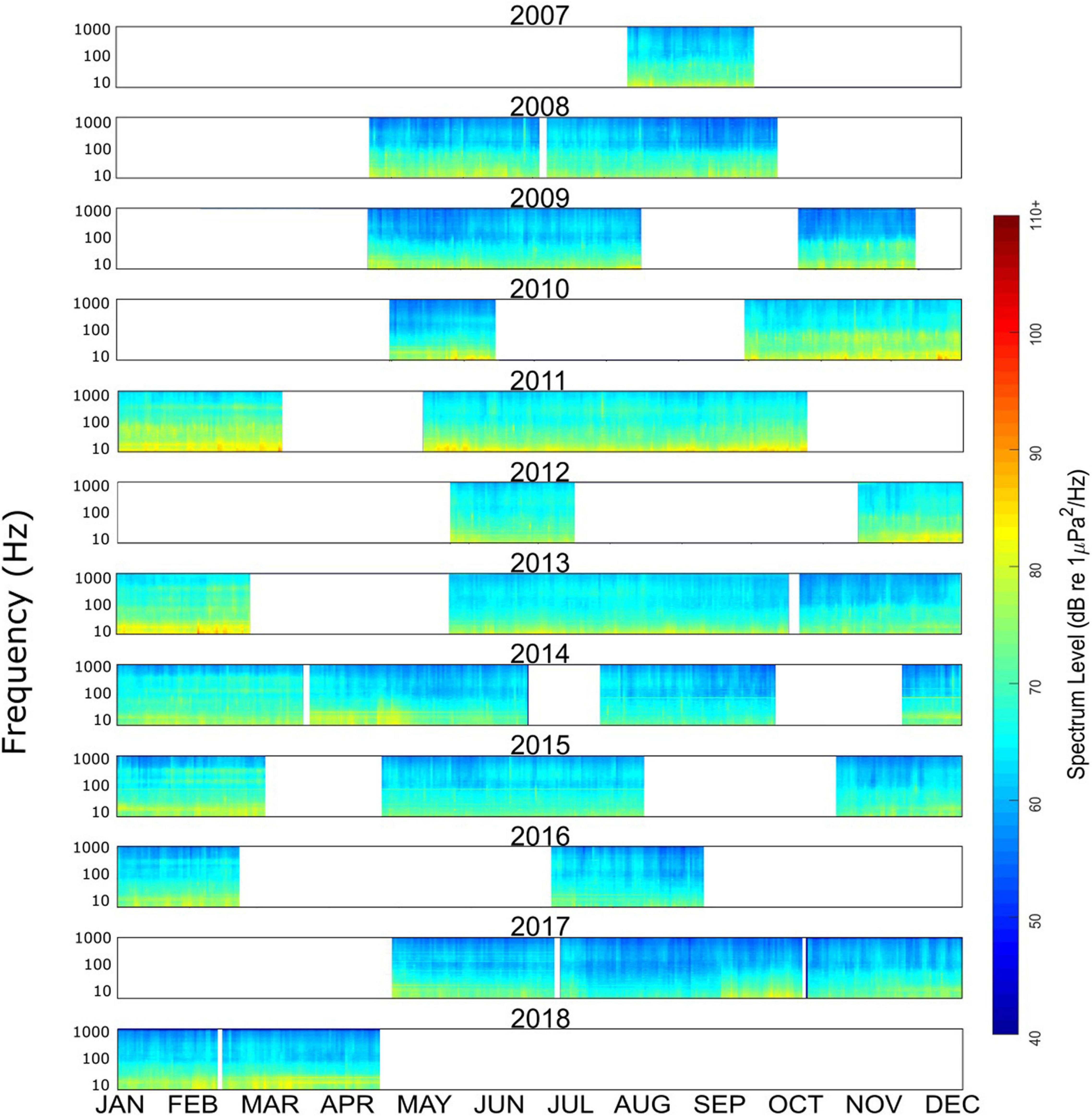
Figure 2. Annual long-term spectral averages over the entire data set from deep water near Kona, Hawai’i. Frequency is along the y-axis (10–1,000 Hz), while time is along the x-axis (Jan–Dec). Sound intensity is shown in color, from lowest (dark blue) to highest (red).
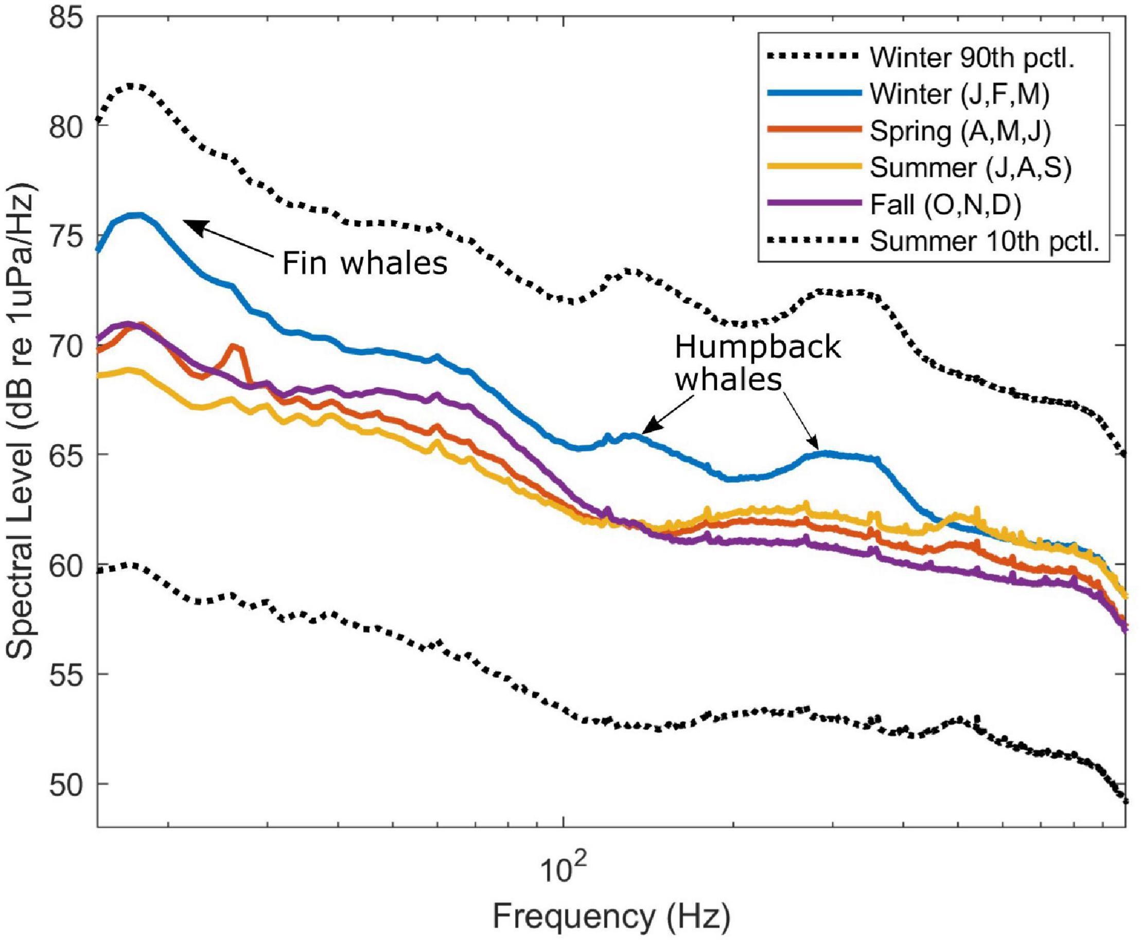
Figure 3. Low-frequency (10–1,000 Hz) spectra from four seasons over all years. Median levels were higher for winter (blue), including a peak around 20 Hz for fin whale calls and peaks in the 100–200 and 300–400 Hz ranges for humpback whales. Variability is indicated by black dotted lines showing the 90th percentile in winter and 10th percentile in summer.
Anthropogenic Signal Detection and Correlated Soundscape Metrics
Vessel Detections
Nearby vessel detections were best correlated with energy in the 4 kHz octave for deployments with continuous data (rho = 0.43, p < 0.0001). For deployments with a long gap between duty cycles (e.g., > 10 min) the correlation dropped significantly, such that across the entire data set the correlation for individual deployments varied widely (rho = 0.02-0.51). There was a strong diel pattern, with vessels detected predominantly between sunrise and sunset (Figure 4), similar to what was seen for the detection of vessel-based echosounder pings (see below). There was no notable seasonality to vessel detections, with consistently high levels of detections all year [average of 14 min of vessel presence per hour (23% of each hour) during daytime hours (06:00–20:00 local time)].
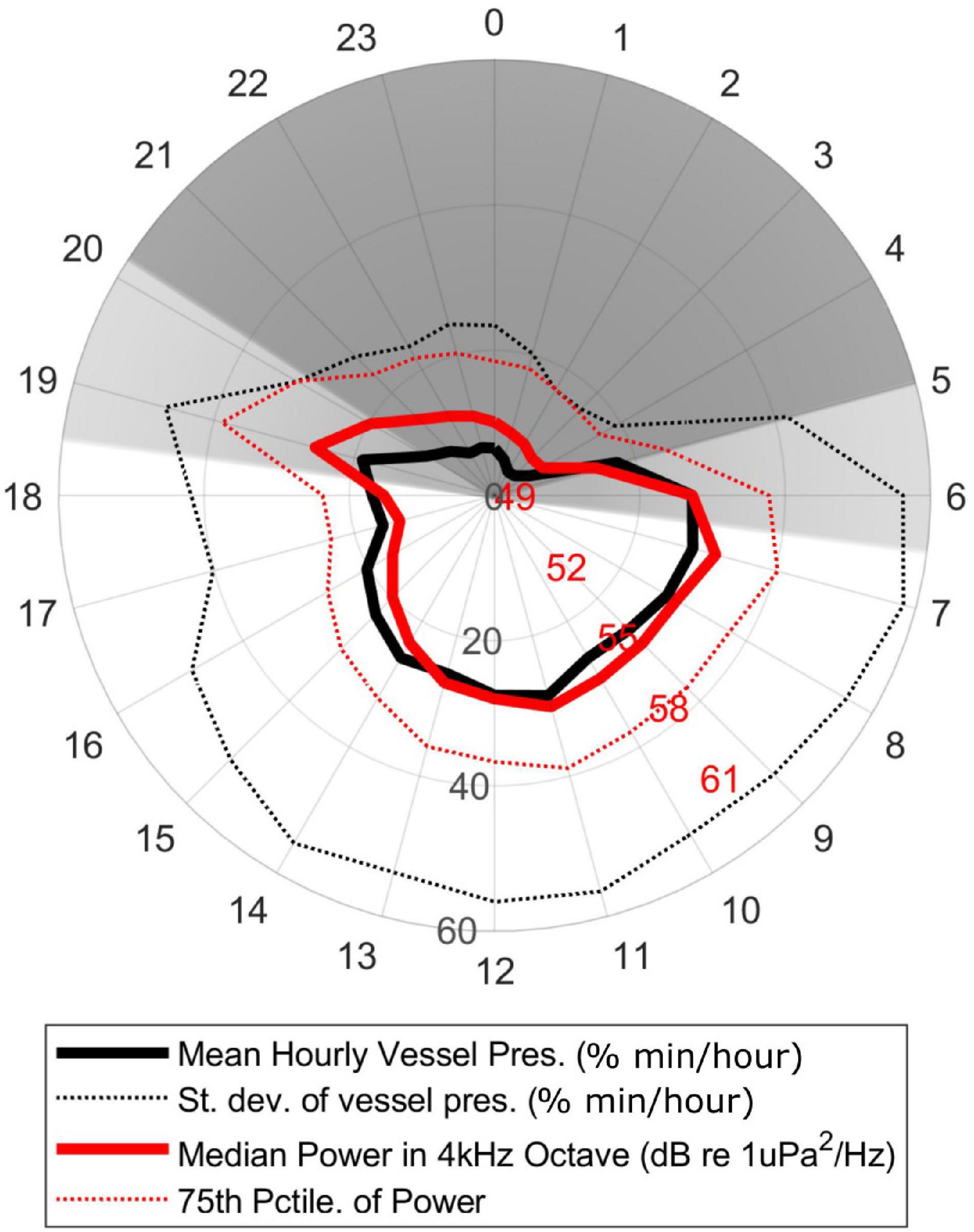
Figure 4. Diel pattern of the average percentage of minutes per hour with nearby vessel detections in continuously sampled deployments (thick black line) and the median sound energy in the 4 kHz octave (thick red line) in the same data per hour of the day local time (HST). The standard deviation of the vessel detections (dotted black line) and 75th percentile of the sound energy (dotted red line) are also shown. Dark gray region indicates nighttime, light gray region indicates dawn/dusk, white region indicates daytime.
Echosounder Pings
A nominal 50 kHz ping was the most commonly detected echosounder frequency. Comparison of the number of echosounder pings per minute in each hour of data and the mean hourly sound energy in a 100 Hz-wide band spanning 50-50.1 kHz revealed a moderate correlation across the entire data set (rho = 0.45, p < 0.0001). There was also a very strong diel pattern, with the vast majority of echosounder pings detected during daylight hours (Figure 5). A seasonal pattern was also evident, with approximately double the number of pings in summer (July-September) than in winter and spring (November-May) (Figure 6). Detailed examination of the echosounder signals over time revealed that the noise from echosounder pings is persistent, with 50% of detections having a received level exceeding 130 dB re 1 μPa.
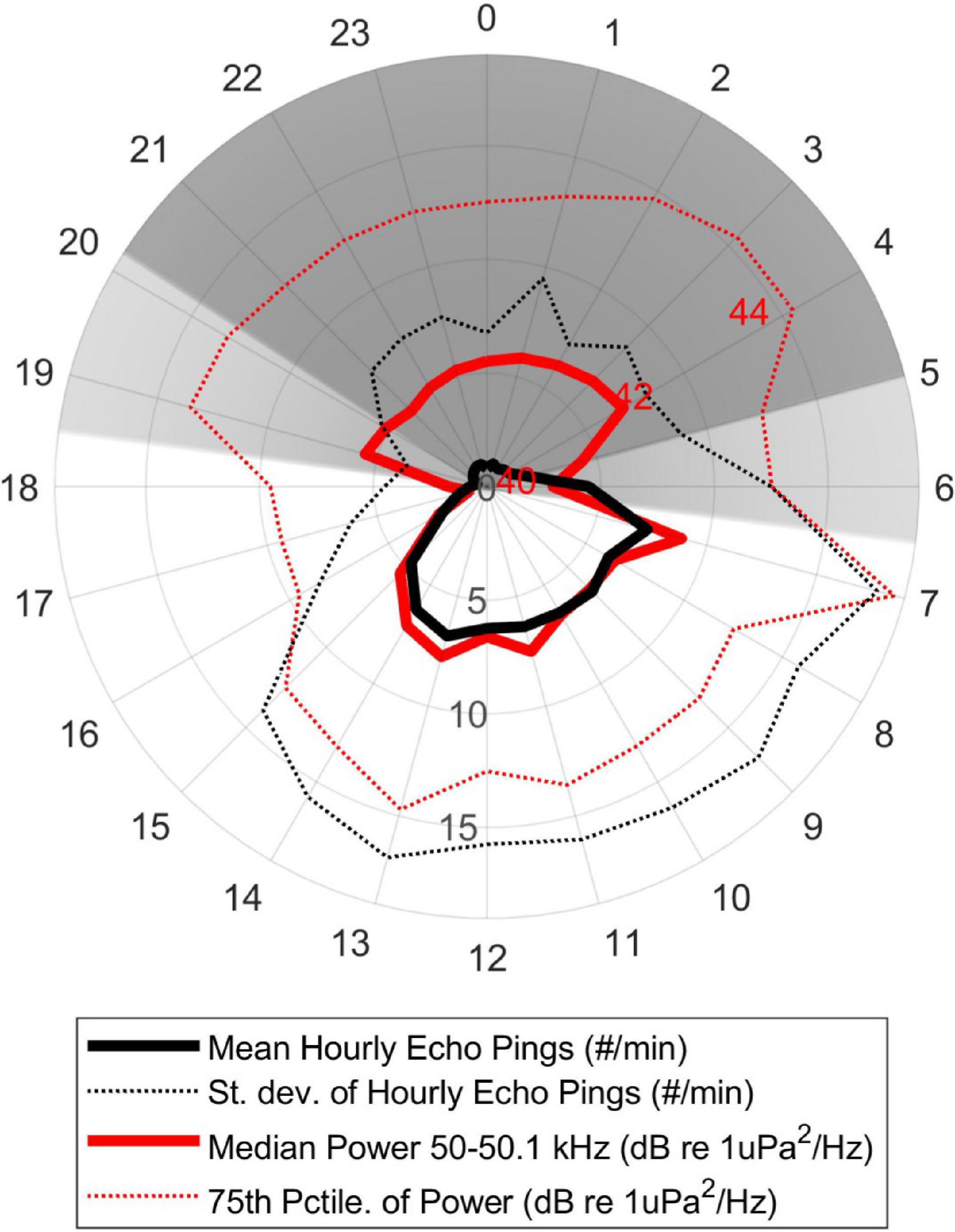
Figure 5. Diel pattern of the average number of echosounder pings per hour (thick black line) and average energy in the 50 kHz band (50.0-50.1 kHz, thick red line). The standard deviation of the echosounder detections (dotted black line) and 75th percentile of the sound energy (dotted red line) are also shown. The majority of nighttime energy in the 50 kHz band is likely due to echolocation clicks from odontocetes, while the “notches” at dawn and dusk in that energy band are due to a decrease in both echosounder ping and odontocete click energy.
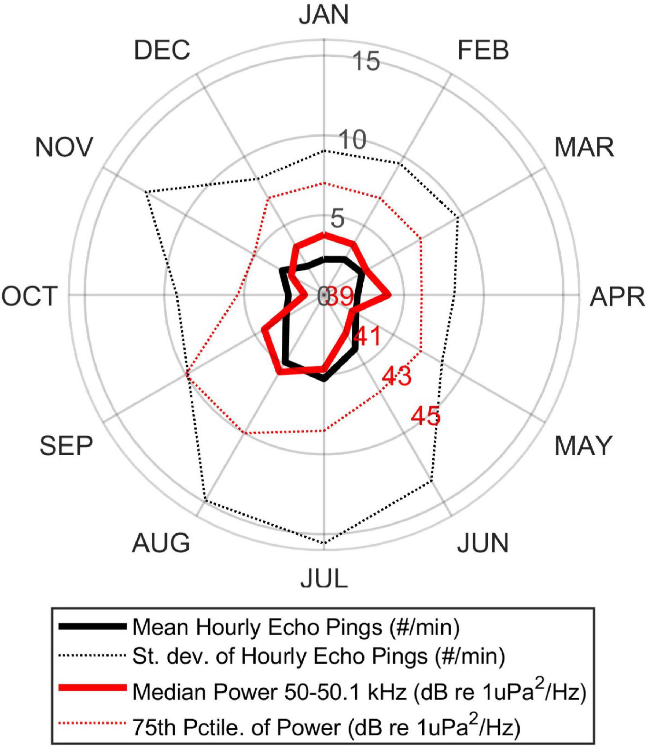
Figure 6. A seasonal pattern is shown for echosounder pings (bold black line) and energy at 50 kHz (50.0-50.1 kHz band, thick red line), with approximately double the number of pings during summer (July and August) compared to the winter and spring (November-May). The standard deviation of the echosounder detections (dotted black line) and 75th percentile of the sound energy (dotted red line) are also shown. Monthly labels located on first day of each month.
Biological Signal Detection and Correlated Soundscape Metrics
Examination of the seasonal spectra (Figure 3) revealed an increase in energy in the winter months (blue spectrum), specifically in the 100-500 Hz band, which corresponds to the presence of humpback whale song. The fall, winter, and spring (October-April) spectra included a peak around 20 Hz, which indicates the presence of fin whale calls (Širović et al., 2013). Additional energy in the low-frequency spectra may be attributable to various fish species, many of which are known to generate a wide variety of sounds. Signal-specific detectors were not implemented for baleen whales other than humpback whales (see below) or for fish sounds, so further analysis of the contribution of these signal types is not included in this study.
Humpback Whale Detections
The automated detections of humpback whales correlated best with the energy in the 125 Hz octave. Although there was only a small correlation when looking at the whole year (rho = 0.22, p < 0.0001), the correlation improved when the data were limited to just the winter months when this species was expected to be present near Hawai’i (rho = 0.30, p < 0.0001). During this season, the increasing energy in this frequency band paralleled the increasing number of humpback-positive-min per day (Figure 7). There was no notable diel pattern in humpback whale detections.
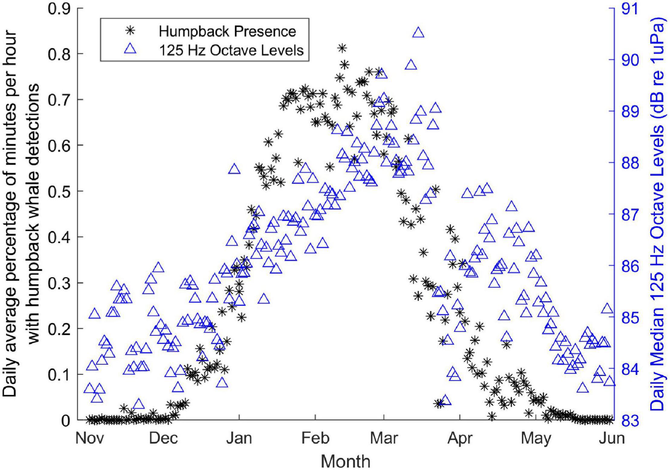
Figure 7. Comparison of mean daily percent of humpback whale positive minutes per hour (black stars, left axis) and median daily 125 Hz octave levels (blue triangles, right axis). Peak presence of humpback whales (mid January-early March) overlaps with the peak energy in the 125 Hz octave (mid February–mid March). Monthly labels located on first day of each month.
Odontocete Click Detections
The clicks of odontocetes were detected throughout the data set, and reveal an intensely nocturnal pattern (Figure 8), with the vast majority of detections happening during dusk and night, less during dawn and day. The energy in the 31.5 kHz octave was well correlated with the number of odontocete positive minutes per hour (rho = 0.50, p < 0.0001). There was no seasonality in odontocete detections.
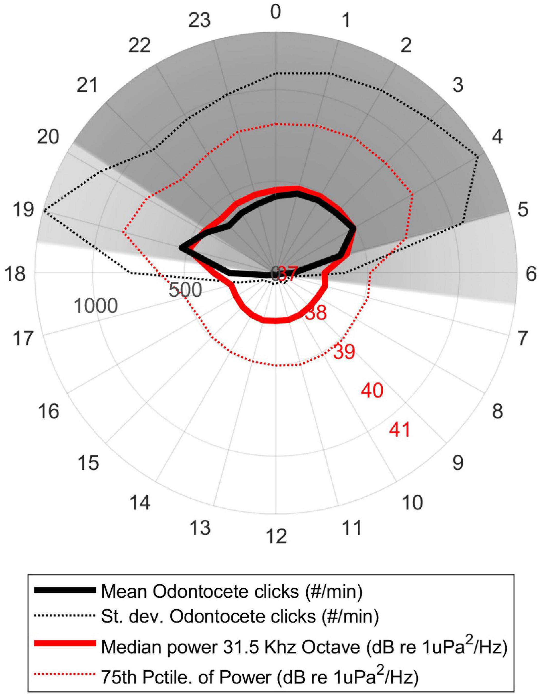
Figure 8. Diel trend in the average number of delphinid echolocation clicks per minute in each hour of the day (thick black line). The average median sound energy in the 31.5 kHz octave, integrating 26–56 kHz (thick red line), in the same data per hour of the day local time (HST). The standard deviation of the delphinid detections (dotted black line) and 75th percentile of the sound energy (dotted red line) are also shown. Dark gray region indicates nighttime, light gray region indicates dawn/dusk, white region indicates daytime.
No Vessel Periods
The duration of the no-vessel periods were approximately 38 h during Iselle and 33 h during Darby. During each of the 2-week periods around each hurricane there was only a slight correlation between the wind speed and the best-correlated soundscape metric (the 1-Hz wide band at 900 Hz, rho = 0.2, p < 0.0001 for each storm). Wideband spectral plots revealed changes in the overall energy levels during the storms (Figure 10). First, both no-vessel periods had lower sound energy during daytime hours between ∼150 and 800 Hz (Figures 10A,B). These are the frequencies with the majority of vessel energy at this site, as shown in the example spectrum and LTSA (Figures 10E,F), which contain a representative hour with typical vessel passages. Second, the storms passed the HARP during different periods of the day, with Iselle present during the daytime (Figure 10A) and Darby present primarily during the nighttime (Figure 10D). During Iselle the storm produced higher energy in frequencies above ∼200 Hz (Figure 10A, red line in red shaded box), but this energy was still not as high as when vessels were present the week before (Figure 10A, black line). In contrast, the energy was elevated at all frequencies above 30 Hz (Figure 10D, red line in shaded box) during the passage of Darby.
Discussion
Long-Term Monitoring of a Deep-Water Marine Soundscape
Motivated by the lack of detailed, wide-band, long-term analysis of marine soundscapes, we set out to assess trends at one nearshore, deep-water site over more than a decade. Here we provide an example of the soundscape in a tropical, deep-water, island-associated habitat, which we hope will be compared to underwater soundscapes from other locations. We looked for cyclical patterns on time scales as short as a day and as long as a year, and documented the sound sources that dominate this soundscape on diel, seasonal and inter-annual time scales at various frequencies, as well as signals that do not dominate the soundscape but contribute to the acoustic environment nonetheless.
The long duration, wide bandwidth, and recording depth of the data in the current soundscape analysis allow us to consider all sound sources within the hearing range of the animals found in this acoustic habitat. The lowest frequency sounds (e.g., 20 Hz) are likely heard by large baleen whales such as blue and fin whales (Erbe, 2002) and may also be sensed by many fish or invertebrates. The highest recorded frequencies (160 kHz) capture signals like the echolocation clicks of Kogia spp. (with energy above 120 kHz) that are above the hearing capabilities of many, but not all, marine mammals (e.g., Szymanski et al., 1999; Li et al., 2011).
In addition to the duration and frequency range of the data set, we were also presented with challenges in how to efficiently analyze the data, considering the total size of the data set and the complexity of the signals present. While a general spectral analysis is useful, and reveals some of the important signals in the soundscape, such as the seasonal presence of humpback whales (Figure 7) or the incessant pinging of echosounders at 50 kHz (Figure 6), much of the detail and nuance is lost in this wide view. To explore some of the smaller-scale details we employed a large suite of analysis tools, each with its own challenges and limitations, and each requiring different levels of human input and expertise. Computer-based methods were essential to analyzing the full data set in a reasonable time frame. A similarly multi-faceted analysis scheme will likely be required for most large-scale, underwater soundscape analysis projects going forward.
The long-term perspective, as shown in the annual long-term spectral averages (Figure 2), allows us to draw some overall conclusions about the soundscape at this location over more than 10 years. Notably absent are strong seasonal or long-term changes, with sound sources and levels being relatively stable and consistent over seasons and years. This is as expected, given the tropical latitude and water depth, which combine to mediate most of the seasonal impacts seen in soundscapes at higher latitudes and/or in shallow water environments (e.g., Haver et al., 2017, 2019). There is a slight seasonal pattern, seen most clearly in the spectra in Figure 3, with increased energy across all frequencies in the winter, likely due to seasonal increases in wind speed and storm-generated noise, as well as localized peaks in the frequencies that correlate with the seasonal presence of humpback and other baleen whale calls. Across all frequencies the wintertime sound energy increase is approximately 2-3 dB. In the long-term view we also notice the consistent presence of energy from vessels (Figure 4), shown as higher energy in lower frequencies (∼150-20 kHz) across all years. With such chronic noise this is clearly not a pristine environment, despite being comparatively remote from continents.
Previous research by Širović et al. (2013) using a subset of these data (∼91 days from fall/winter of 2009, 2010 and 2011, 10-1,000 Hz frequency band) provided some initial findings, upon which we expanded. We found similar seasonal patterns, particularly the winter presence of humpback and fin whales. We also confirmed their initial findings of increased energy during daytime hours. We can attribute that increase to vessel presence based on our vessel and echosounder detections. Širović et al. (2013) identified a daily peak in energy at 500 Hz around 20:00 local time, which is also revealed in our data in the nighttime spectra in Figures 10C,D and as a pulse of energy seen just after sunset in the LTSAs for each hurricane passage (Figure 9). The exact source of this signal remains unknown, but its daily cycle and diffuse energy suggest it may be related to a fish chorus or other daily behavior, such as a diel vertical migration.
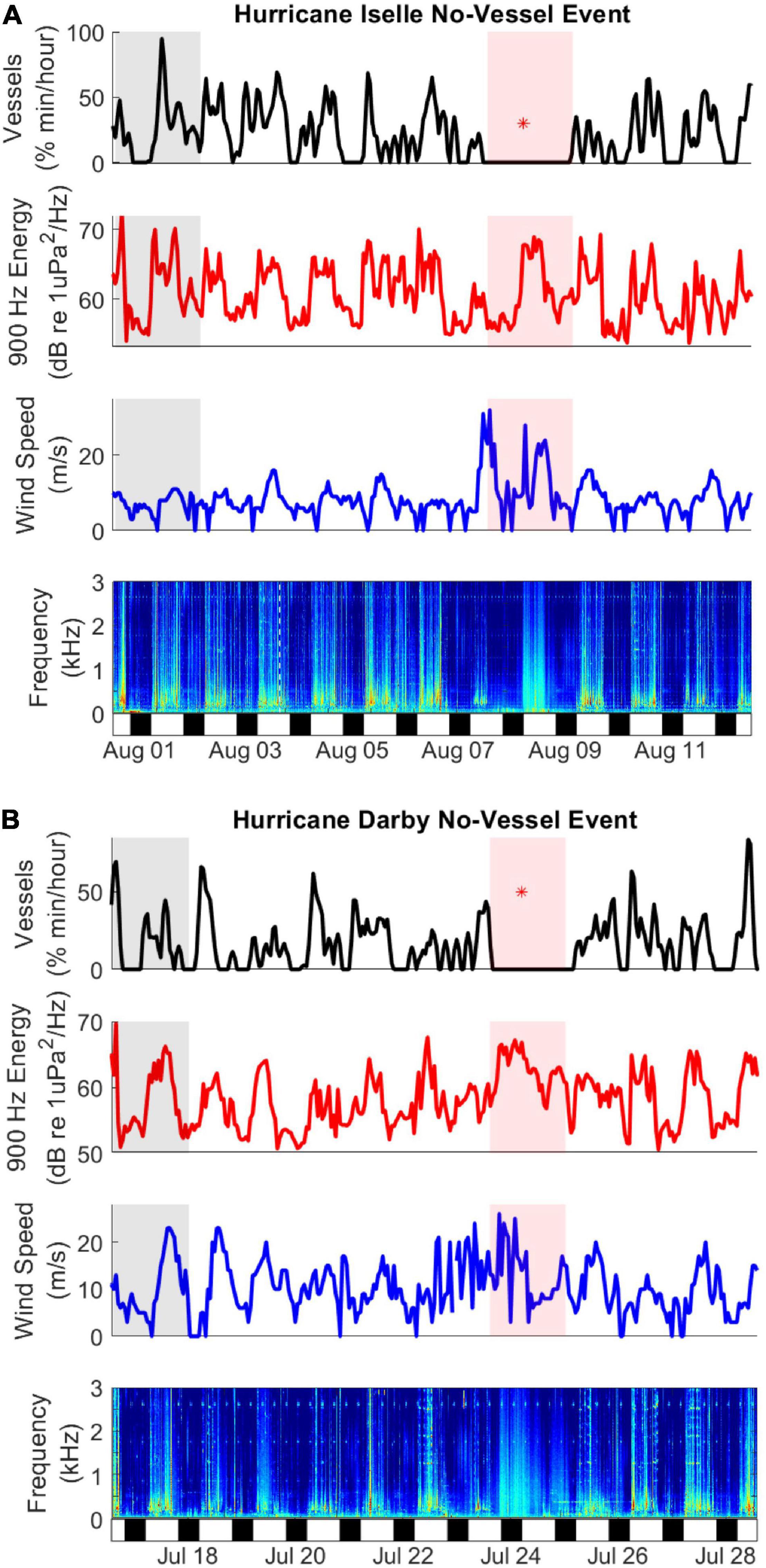
Figure 9. No-Vessel Events during Hurricane Iselle (A) and Hurricane Darby (B). The pale red rectangle indicates the no-vessels event, pale gray rectangle indicates the period from 1 week prior, which is also plotted in Figure 10. Red star (*) in the top sub-plots indicates the time of closest approach of the hurricanes to the HARP. Sub-plots include smoothed vessels detections (black line, percent of minutes per hour with detections, 4-h smoothing window), energy in a 1 Hz band spanning 900-901 Hz (red line, dB re μPa2/Hz), wind speed (blue line, meters/second), and a long term spectrogram from 0 to 3 kHz, with sound intensity indicated by color, from least intense (blue) to most intense (red). Night and day phases are indicated by the bottom bar, with black representing night and white indicating dawn, day and dusk.
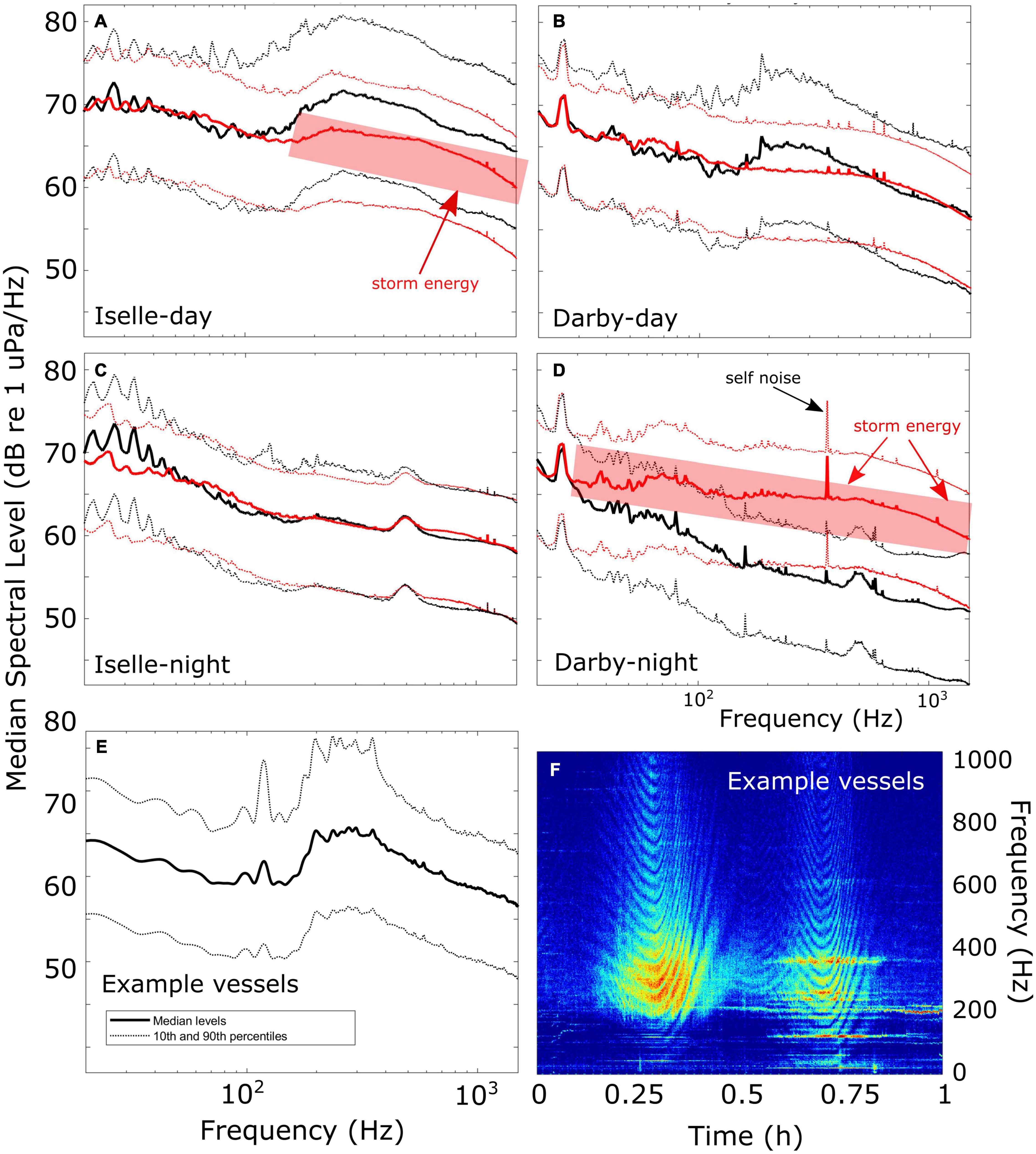
Figure 10. Median spectra (20–1,500 Hz) during the no-vessel periods (red) of Hurricanes Iselle (A,C) and Darby (B,D) and corresponding day and night from a period 1 week prior to the storms (black), with 10th and 90th percentiles (dotted lines) to indicate variability. Periodic spikes in spectra are due primarily to HARP self-noise and do not represent signals in the broader environment. See (D) for labeled example. Elevated spectral levels due to storm energy are indicated by red shaded boxes (A,D). Also shown are spectra (E) and a spectrogram (F) for an example hour with vessel passages that are typical of this data set, having minimal energy below 150 Hz.
Contributions of Anthropogenic Signals
The nearshore waters of Hawai’i are much-used for many human activities, most of which generate underwater noise. The diurnal presence of vessels and echosounder pings (Figures 4, 6) was expected, given the known diurnal patterns of humans in the area. Such diel trends have been documented in this soundscape at lower frequencies (∼500 Hz) by Širović et al. (2013). However, the extent and persistence of the acoustic presence was remarkable. The chronic daytime vessel noise is likely coming from both smaller sport-fishing as well as commercial fishing vessels. The typical schedule of these vessels is to depart a nearby harbor each morning around sunrise, travel to various established fishing locations, including a fish aggregating device that is located in the same area as the HARP, and then return to shore in the evening.
Despite being over deep water, sounds from these vessels, particularly propeller cavitation and engine noise, introduce acoustic energy into the local environment as revealed by the constant, lower frequency (< 5,000 Hz) energy in our data (Figures 2, 4). Although the duration of each vessel passage is relatively short (∼15-30 min), the number of encounters per day (∼1-5 per hour during daylight hours, for an average of 14 min of vessel presence per hour during daytime hours, reveals the considerable impact this sound source may have on the area across a wide frequency band (10 Hz-50 kHz), similar to what was found by Putland et al. (2017). Also, given the broadband nature of these signals, they are likely to cause significant masking for many marine animals, including protected marine mammal species, whose acoustic signals and hearing ranges fall well within this frequency band (e.g., humpback, pilot, killer and sperm whales, etc.).
We found that the frequency spectra produced by most vessels in our data was different from what is typically described for underwater commercial vessels. Unlike large ships that have considerable energy below 100 Hz (e.g., McKenna et al., 2012b and McKenna et al., 2013), the energy in the vast majority of vessel passages near the Hawai’i HARP peaked between 200 and 400 Hz, and dropped off below 150 Hz (Figure 10E,F). This may be a result of propagation, or due to the majority of vessels being smaller in size, or a combination thereof. This difference in sound signature may help explain a lack of correlation found by Širović et al. (2013) who found no relationship between the energy in a 40 Hz band at this site and the presence of vessels detected using the Automated Identification System (AIS). If most of the vessels passing this site are smaller it is likely that they do not transmit AIS signals. Therefore they would not be included in any AIS-based monitoring, as was found by Magnier and Gervaise (2020), who determined that less than 4% of vessels near their site in the Pelagos marine sanctuary in the Mediterranean were using AIS systems. Similarly, Cholewiak et al. (2018) determined that non-AIS vessels contributed significantly to the noise in the Stellwagen National Marine Sanctuary, reducing the communication space of baleen whales by approximately 30%. Similar conditions may be impacting the cetaceans off Hawai’i, and should be taken into consideration when assessing the environmental impacts of any noise-generating human activities.
In contrast to the broadband signals from vessel engines and propeller cavitation, echosounder pings are very narrow band, with each ping generally being only a few Hertz in bandwidth. However, despite the limited frequency band, the signals have considerable energy, with a median energy per ping being 130 dB re 1 μPa at this site. Echosounder pings have not been reported in other soundscape studies, perhaps because they tend to be above the frequency range of many passive acoustic monitoring systems. Yet, the frequencies of these pings and the side-lobes of higher frequency pings are within the hearing range of many marine mammals, particularly odontocetes (Deng et al., 2014). The biological impact of the near-constant daytime pinging at this location should not be underestimated and may be impacting marine mammals in the area. It is fortunate that there appears to be some temporal acoustic niche separation, with anthropogenic noise not overlapping with the majority of echolocation clicks from delphinids, because of their nocturnal behavior (Figures 4, 5, 8). However, the possibility of significant physical or acoustic interactions during dawn and dusk should be explored further, and anthropogenic noise may still impact their daytime resting even when they are less acoustically active. Additionally, several species of odontocetes are active and detected at this site during all hours of day and night (e.g., Baumann-Pickering et al., 2014; Merkens et al., 2019), increasing the chances of acoustic overlap and masking for those species.
We observed a seasonal trend in echosounder pings, with an approximate doubling of detections during summer months (June–September) (Figure 6). This likely reflects the seasonality of tourism as well as chances of good weather, both of which are higher during the summer. The corresponding lack of a seasonal pattern for vessel detections may be the result of echosounders pinging while vessels are moving slowly or drifting and therefore not generating detectable levels of sound energy. This disconnect may also be due to the detector function, where the threshold for “presence” shifts dynamically based on the overall energy in each individual 2-h window. Windows with almost no vessel noise and a single higher-energy passage (e.g., during a month with less overall vessel activity) might result in a similar detection rate as windows with a high baseline of vessel noise (e.g., during peak summer months) and a single higher-energy passage. Despite this potential limitation in detector performance there are currently no other options available for automated detection of vessels, and overall performance was found to be satisfactory by validating a subset of manual vessel detections. Further analysis to assess the impacts of this dynamic detection method and improvement of this detector are beyond the scope of the current work.
We considered whether soundscape metrics could be used as a proxy for anthropogenic signals, and found that this depends greatly on the signal type and the detection method. The automated vessel detections (Figure 4), may work well at a location where the vessel passages are distinct from each other and when analyzing a continuous recording, which could result in a high correlation with the soundscape metrics (e.g., energy in the 4 kHz octave). However, when the data are duty cycled, or there is a constant, high level of vessel energy, the correlation suffers. This varying performance reveals that the soundscape metrics could possibly be used as a proxy for vessel passages, but more importantly, the impact of recording parameters and ambient noise conditions on detector performance should be considered. In contrast, detection of the echosounders was much more consistent across time and with low variability in ambient noise conditions at higher frequencies, resulting in a strong correlation between the soundscape metric (50-50.1 kHz band) and the automatic detections. In this case, the sound energy measurements can be used reliably for monitoring the presence of echosounder pings over time.
The Contribution of Biological Signals
While anthropogenic sounds were shown to be prevalent throughout the time series, biological sounds are also significant contributors to the soundscape at this location. The dominant driver of seasonal change in frequencies below 1,000 Hz was the wintertime songs of humpback whales (Figures 3, 7). These results confirm the earlier findings by Širović et al. (2013), who found humpback whales and other baleen whale species were an important component of the soundscape at multiple sites in the North Pacific.
Our analysis revealed only a small correlation between automated humpback whale detections and soundscape metrics, which have been used by other researchers to monitor and quantify humpback whale presence at other locations in the Hawaiian Islands (e.g., Au et al., 2000; Kügler et al., 2020). There were likely other sound sources in our data set contributing to the 125 Hz octave levels, adding to the signals of the whales in this band. There was possibly less energy from humpbacks at this location as chorusing generally occurs in shallower water. Perhaps most importantly, the humpback whale detector determined presence or absence of humpback calls in a 75-s bin and did not indicate the total number of calls in that bin. Call counts may correlate more closely with sound energy in that frequency band.
Another question to be explored is why humpback whale detections correlated best with the energy in the 125 Hz octave, when those calls are known to primarily span 200-1,000 Hz. One possible explanation is that the energy of vessels dominates the daytime soundscape between 150 and 1,000 Hz at this site, as described above. Given this potential masking, the frequencies just below the vessel energy may contain enough energy from humpback whales to produce a correlation. Examination of the correlation at a site without intense vessel noise may reveal a stronger relationship between humpback whale calls and the energy in a higher frequency band (e.g., the 250 or 500 Hz octaves).
Two additional details related to humpback whale detection patterns are revealed through examination of Figure 7. There is a subtle mismatch between the seasonal peak in the 125 Hz octave levels and the peak of humpback whale presence, and there are a few unexpectedly low soundscape metric levels in March and April. The overall mismatches are likely a result of the poor correlation between these two parameters, described above, particularly due to the methods of the humpback whale call detector, which does not discriminate between one whale call and many calls per 75-s window. The peak in the number of calls per hour may be more aligned with the peak in the 125 Hz band, but those measurements are not possible at this time. The low levels in March and April are likely an artifact of non-uniform sampling over time. As revealed in Figure 2, there is limited coverage of March and early April across the 11 years of monitoring, resulting in greater variability of all measurements during those months. Ongoing monitoring at this site during the spring months will hopefully reduce variability and reveal a clearer trend in both parameters.
In contrast to the humpback whales, our odontocete detections showed no seasonal trend, but were highly nocturnal. Although we did not identify the exact species present, many of the odontocetes in this region that produce clicks in the frequencies targeted by our automated detector (∼5–90 kHz) are primarily delphinids, some of which are known to have strong diel behavioral and acoustic cycles (e.g., Norris and Dohl, 1980; Lammers, 2004; Benoit-Bird and Au, 2009; Soldevilla et al., 2010; Wiggins et al., 2013). Most of these species are primarily nocturnal, with increased foraging at night and resting during the day. Because they rely heavily on echolocation for foraging, this behavioral pattern leads to increased acoustic activity at night (e.g., Henderson et al., 2011), which was very clear in our data set (Figure 8). The moderate correlation between the detection of odontocetes and the sound energy in an overlapping frequency band (31.5 kHz octave) indicates that the presence of odontocetes could be monitored using soundscape metrics as a proxy. Although the delphinids’ nocturnal behavior provides some temporal niche separation from the majority of anthropogenic activities and their associated sounds, there is overlap between these two signals during dawn and dusk, which may present opportunity for physical and/or acoustic interactions during these times. It is important to acknowledge that we did not include an analysis of delphind whistles in this study, and although the presence of whistles is very closely linked to echolocation activity for monitoring dolphin presence, we have not explored the contribution of this signal type to the overall soundscape.
No Vessel Periods
Two unique opportunities to explore the soundscape in the absence of anthropogenic noise (no close vessels or echosounder pings) arose from the passages of two hurricanes during the monitoring period (Figures 9, 10). The eyes of hurricanes Iselle (2014) and Darby (2016) passed close to the HARP (within 20–30 km) as the storms each moved past the southern end of the island of Hawai’i.
Iselle moved by the HARP during daytime hours, so the sound energy from wind and rain was present during the daytime (Figure 10A), and was nearly absent from the nighttime soundscape (Figure 10C). This revealed that the storm was characterized by broadband energy at frequencies of approximately 150 Hz and higher (Figure 10A, red), but that the noise from this storm was not higher energy than the typical noise from vessels in those same frequencies (Figure 10A, black).
In contrast, Darby was present near the HARP primarily at night, so we saw lower levels across all frequencies in the daytime spectra due to the absence of vessels (Figure 10B, red), and very elevated levels across all frequencies above 40 Hz in the nighttime spectra due to the storm (Figure 10D, red). This aligns generally with the results of Wiggins et al. (2016) who found a marked increase in sound energy above 300 Hz during the passage of a hurricane close to a HARP in the Gulf of Mexico. Examination of the LTSAs in Figure 9 show that the sound from the storms is slightly different from the daily sounds of vessels, with energy distributed more diffusely across a wider frequency range.
There was a small correlation between wind speeds and sound energy levels at 900 Hz, which was the frequency band with the highest correlation of any of the bands that were tested. This soundscape metric appears to be a combination of energy from both wind and vessels, as shown in Figure 9, such that it reflects vessel presence when vessels are present (e.g., daytime) and reflects wind energy when vessels are absent (e.g., nighttime or during a no-vessel event). The overall low correlation between wind speed and the soundscape metric is likely due to masking of the dominant wind frequencies by vessel noise and to local variations in wind speed due to the topography of the island of Hawai’i, as well as the distance between the HARP site and the nearest wind speed monitoring station, which is onshore at the Kona International Airport.
The passages of both hurricanes also revealed some nuanced human behavior. On one hand, people were eager to maximize time at sea, with vessels present as soon as sunrise on the day after the storms passed. In contrast, the uncertainty and risks associated with the passage of a hurricane are highlighted by examining the time series of wind speed during Hurricane Darby (Figure 9B). Wind speeds were highly variable during the storm, but were not notably higher than a week prior, yet vessels did not leave the dock during the storm. This discrepancy may also be impacted by the issues associated with the wind speed monitoring station described above. Whatever the cause, it seems that wind speeds are not a direct correlate to the presence or absence of vessels.
It is clear that during both Hawaiian hurricanes the absence of vessels had a large impact on the soundscape, even if the addition of sound energy from the storms themselves prevented an assessment of daytime ambient noise under lower wind conditions.
Conclusion
In conclusion, we have shown that the soundscape off Hawai’i, monitored for more than a decade, includes a large variety of sound sources, some with clear patterns over diel and seasonal scales. This exceptionally large data set required analysis using both manual and automated methods, and we have demonstrated multiple tools that could be used to explore similar trends over short and long time scales in other data. The variability in the presence of sound sources over these different time scales must be considered when attempting to use passive acoustics for long-term monitoring or abundance estimation, and when assessing how anthropogenic activity may be impacting marine animals. We hope future soundscape studies will attempt to monitor over long time periods and across wide frequency bands, particularly in the mostly-unexplored deep ocean that covers the majority of the surface of the Earth.
Data Availability Statement
Publicly available datasets were analyzed in this study. These data can be accessed at the NCEI Passive Acoustic Data Map Viewer at this doi: https://doi.org/10.25921/PF0H-SQ72.
Author Contributions
KM, SB-P, and EO contributed to the conception and design of the study. KM, SB-P, MZ, JT, and AA performed the analyses. KM wrote the first draft of the manuscript. SB-P, MZ, JT, and AA wrote sections of the manuscript. All authors contributed to manuscript revision, read, and approved the submitted version.
Funding
Funding for HARP deployment and data analysis has been provided by the Protected Species Division and the Ecosystems and Oceanography Division at NMFS PIFSC, the Ocean Acoustics Program at the NMFS Office of Science and Technology, and by the United Sates Navy CNO-N45 and the Pacific Fleet.
Conflict of Interest
KM was employed by company Saltwater Inc.
The remaining authors declare that the research was conducted in the absence of any commercial or financial relationships that could be construed as a potential conflict of interest.
Publisher’s Note
All claims expressed in this article are solely those of the authors and do not necessarily represent those of their affiliated organizations, or those of the publisher, the editors and the reviewers. Any product that may be evaluated in this article, or claim that may be made by its manufacturer, is not guaranteed or endorsed by the publisher.
Acknowledgments
We would like to thank many people for their efforts in data collection and assistance with analysis tool development. In particular Erik Norris for his work on hardware maintenance and many instrument deployments and recoveries, and Sean Wiggins for the development and ongoing improvements of the HARPs. Many of the deployments and recoveries were made possible by the efforts of Robin Baird, Daniel Webster, Greg Schorr, and Dan McSweeney.
Footnotes
References
Allen, A. N., Harvey, M., Harrell, L., Jansen, A., Merkens, K. P., Wall, C. C., et al. (2021). A Convolutional neural network for automated detection of humpback whale song in a diverse, long-term passive acoustic dataset. Front. Mar. Sci. 8:607321. doi: 10.3389/fmars.2021.607321
Andrew, R. K., Howe, B. M., Mercer, J. A., and Dzieciuch, M. A. (2002). Ocean ambient sound: comparing the 1960s with the 1990s for a receiver off the California coast. Acoust. Res. Lett. Online 3, 65–70. doi: 10.1121/1.1461915
Au, W. W. L. (1993). “Biosonar discrimination, recognition, and classification,” in The Sonar of Dolphins, (New York: Springer), 177–215.
Au, W. W. L., Mobley, J., Burgess, W. C., Lammers, M. O., and Nachtigall, P. E. (2000). Seasonal and diurnal trends of chorusing humpback whales winter in waters off western Maui. Mar. Mamm. Sci. 16, 530–544. doi: 10.1111/j.1748-7692.2000.tb00949.x
Baird, R. W., Webster, D. L., Aschettino, J. M., Schorr, G. S., and McSweeney, D. J. (2013). Odontocete cetaceans around the main Hawaiian Islands: habitat use and relative abundance from small-boat sighting surveys. Aquat. Mamm. 39, 253–269. doi: 10.1578/am.39.3.2013.253
Baumann-Pickering, S., Simonis, A. E., Roch, M. A., McDonald, M. A., Solsona Berga, A., Oleson, E. M., et al. (2014). Spatio-temporal patterns of beaked whale echolocation signals in the North Pacific. PLoS One 9:e86072. doi: 10.1371/journal.pone.0086072
Benoit-Bird, K. J., and Au, W. W. L. (2009). Cooperative prey herding by the pelagic dolphin, Stenella longirostris. J. Acoust. Soc. Am. 125, 125–137. doi: 10.1121/1.2967480
Bertucci, F., Parmentier, E., Lecellier, G., Hawkins, A. D., and Lecchini, D. (2016). Acoustic indices provide information on the status of coral reefs: an example from Moorea Island in the South Pacific. Sci. Rep. 6:33326. doi: 10.1038/srep33326
Buscaino, G., Ceraulo, M., Pieretti, N., Corrias, V., Farina, A., Filiciotto, F., et al. (2016). Temporal patterns in the soundscape of the shallow waters of a Mediterranean marine protected area. Sci. Rep. 6:34230. doi: 10.1038/srep34230
Chapman, N. R., and Price, A. (2011). Low frequency deep ocean ambient noise trend in the Northeast Pacific Ocean. J. Acoust. Soc. Am. 126, EL161–EL165. doi: 10.1121/1.3567084
Chapuis, L., and Bshary, R. (2010). Signalling by the cleaner shrimp Periclimenes longicarpus. Anim. Behav. 79, 645–647. doi: 10.1016/j.anbehav.2009.12.012
Cholewiak, D., Clark, C. W., Ponirakis, D., Frankel, A., Hatch, L. T., Risch, D., et al. (2018). Communicating amidst the noise: modeling the aggregate influence of ambient and vessel noise on baleen whale communication space in a national marine sanctuary. Endanger. Species Res. 36, 59–75. doi: 10.3354/esr00875
Coquereau, L., Lossent, J., Grall, J., and Chauvaud, L. (2017). Marine soundscape shaped by fishing activity. R. Soc. Open Sci. 4:160606. doi: 10.1098/rsos.160606
Dekeling, R. P. A., Tasker, M. L., Van der Graaf, A. J., Ainslie, M. A., Andersson, M. H., André, M., et al. (2014). Monitoring Guidance for Underwater Noise in European Seas, Part I: Executive Summary. Luxembourg: Publications Office of the European Union.
Deng, Z. D., Southall, B. L., Carlson, T. J., Xu, J., Martinez, J. J., Weiland, M. A., et al. (2014). 200 kHz commercial sonar systems generate lower frequency side lobes audible to some marine mammals. PLoS One 9:e95315. doi: 10.1371/journal.pone.0095315
Dziak, R. P., Haxel, J. H., Matsumoto, H., Lau, T., Heimlich, S., Nieukirk, S., et al. (2017). Ambient sound at challenger deep. Mariana Trench. Oceanogr. 30, 186–197.
Erbe, C., Verma, A., McCauley, R., Gavrilov, A., and Parnum, I. (2015). The marine soundscape of the Perth Canyon. Prog. Oceanogr. 137, 38–51. doi: 10.1016/j.pocean.2015.05.015
Fine, M. L., Winn, H. E., and Olla, B. L. (1977). “Communication in Fishes,” in How Animals Communicate, ed. T. A. Sebeok (Bloomington: Indiana University Press), 472–518.
Gedamke, J., Harrison, J., Hatch, L., Angliss, R., Barlow, J., Berchok, C., et al. (2016). Ocean Noise Strategy Roadmap. Available Online at: http://cetsound.noaa.gov/road-map [accessed May 1, 2019].
George, J. C., Clark, C., Carroll, G. M., and Ellison, W. T. (1989). Observations on the ice-breaking and ice navigation behavior of migrating bowhead whales (Balaena mysticetus) near Point Barrow, Alaska, spring 1985. Arctic 42, 24–30.
Harris, H. A., Shears, N. T., and Radford, C. A. (2016). Ecoacoustic indices as proxies for biodiversity on temperate reefs. Methods Ecol. Evol. 7, 713–724. doi: 10.1111/2041-210x.12527
Hatch, L. T., Wahle, C. M., Gedamke, J., Harrison, J., Laws, B., Moore, S. E., et al. (2016). Can you hear me here? Managing acoustic habitat in US waters. Endanger. Species Res. 30, 171–186. doi: 10.1002/ece3.2228
Haver, S. M., Fornet, M. E. H., Dziak, R. P., Gabriele, C., Gedamke, J., Hatch, L. T., et al. (2019). Comparing the underwater soundscapes of four U.S. National Parks and Marine Sanctuaries. Front. Mar. Sci. 6:500. doi: 10.3389/fmars.2019.00500
Haver, S. M., Gedamke, J., Hatch, L. T., Dziak, R. P., Van Parijs, S., McKenna, M. F., et al. (2018). Monitoring long-term soundscape trends in U.S. Waters: the NOAA-NPS Ocean Noise Reference Station Network. Mar. Policy 90, 6–13. doi: 10.1016/j.marpol.2018.01.023
Haver, S. M., Klinck, H., Nieukirk, S. L., Matsumoto, H., Dziak, R. P., and Miksis-Olds, J. L. (2017). The not-so-silent world: measuring Arctic, Equatorial, and Antarctic soundscapes in the Atlantic Ocean. Deep Sea Res. I 122, 96–104.
Haxel, J., Dziak, R. P., and Matsumoto, H. (2013). Observations of shallow water marine ambient sound: the low frequency underwater soundscape of the central Oregon coast. J. Acoust. Soc. Am. 133, 2586–2596. doi: 10.1121/1.4796132
Heenehan, H. L., Van Parijs, S. M., Bejder, L., Tyne, J. A., Southall, B. L., Southall, H., et al. (2017). Natural and anthropogenic events influence the soundscapes of four bays on Hawaii Island. Mar. Pollut. Bull. 124, 9–20. doi: 10.1016/j.marpolbul.2017.06.065
Henderson, E. E., Hildebrand, J. A., Smith, M. H., and Falcone, E. A. (2011). The behavioral context of common dolphin (Delphinus sp.) vocalizations. Mar. Mamm. Sci. 28, 439–460. doi: 10.1111/j.1748-7692.2011.00498.x
Hermannsen, L., Mikkelsen, L., Tougaard, J., Beedholm, K., Johnson, M., and Madsen, P. T. (2019). Recreational vessels without Automatic Identification System (AIS) dominate anthropogenic noise contributions to a shallow water soundscape. Sci. Rep. 9:15477. doi: 10.1038/s41598-019-51222-9
Hildebrand, J. A. (2009). Anthropogenic and natural sources of ambient noise in the ocean. Mar. Ecol. Prog. Series 395, 5–20. doi: 10.3354/meps08353
Hildebrand, J. A., Frasier, K. E., Baumann-Pickering, S., and Wiggins, S. M. (2021). An empirical model for wind-generated ocean noise. J. Acoust. Soc. Am. 149, 4516–4533.
Janik, V. M., and Sayigh, L. S. (2013). Communication in bottlenose dolphins: 50 years of signature whistle research. J. Comp. Physiol. A 199, 479–489. doi: 10.1007/s00359-013-0817-7
Jaquet, N., Dawson, S., and Douglas, L. (2001). Vocal behavior of male sperm whales: why do they click? J. Acoust. Soc. Am. 209, 2254–2259. doi: 10.1121/1.1360718
Ketten, D. R. (1994). Functional analyses of whale ears: adaptations for underwater hearing. Proc. Underw. Acoust. 1, 264–270. doi: 10.1007/978-1-4939-2981-8_64
Krause, B. L. (2008). Anatomy of the soundscape: evolving perspectives. J. Audio. Eng. Soc. 56, 73–80.
Kügler, A., Lammers, M. O., Zang, E. J., Kaplan, M. B., and Mooney, A. T. (2020). Fluctuations in Hawaii’s humpback whale Megaptera novaeangliae population inferred from male song chorusing off Maui. Endanger. Species Res. 43, 421–434. doi: 10.3354/esr01080
Lammers, M. O. (2004). Occurrence and behavior of Hawaiian spinner dolphins (Stenella longirostris) along Oahu’s leeward and south shores. Aquat. Mamm. 30, 237–250. doi: 10.1578/am.30.2.2004.237
Li, S., Nachtigall, P. E., and Breese, M. (2011). Dolphin hearing during echolocation: evoked potential responses in an Atlantic bottlenose dolphin (Tursiops truncatus). J. Exp. Biol. 214, 2027–2035. doi: 10.1242/jeb.053397
Magnier, C., and Gervaise, C. (2020). Acoustic and photographic monitoring of coastal maritime traffic: influence on the soundscape. J. Acoust. Soc. Am. 147, 3749–3757. doi: 10.1121/10.0001321
Mann, D. A., Caster, B. M., Boyle, K. S., and Tricas, T. C. (2007). On the attraction of larval fishes to reef sounds. Mar. Ecol. Prog. Ser. 388, 307–310.
Marley, S. A., Erbe, C., and Salgado-Kent, C. P. (2016). Underwater sound in an urban estuarine river: sound sources, soundscape contribution, and temporal variability. Acoust. Aust. 44, 171–186. doi: 10.1007/s40857-015-0038-z
Marley, S. A., Salgado Kent, C. P., Erbe, C., and Thiele, D. (2017). A tale of two soundscapes: comparing the acoustic characteristics of Urban versus pristine coastal dolphin habitats in Western Australia. Acoust. Aust. 45, 159–178. doi: 10.1007/s40857-017-0106-7
Mathias, D., Gervaise, C., and Di Iorio, L. (2016). Wind dependence of ambient noise in a biologically rich coastal area. J. Acoust. Soc. Am. 139, 839–850. doi: 10.1121/1.4941917
McDonald, M. A., Hildebrand, J. A., and Wiggins, S. M. (2006). Increases in deep ocean ambient noise in the Northeast Pacific west of San Nicolas Island, California. J. Acoust. Soc. Am. 120, 711–718. doi: 10.1121/1.2216565
McKenna, M. F., Katz, S. L., Wiggins, S. M., Ross, D., and Hildebrand, J. A. (2012a). A quieting ocean: unintended consequence of a fluctuating economy. J. Acoust. Soc. Am. 132, EL169–EL175. doi: 10.1121/1.4740225
McKenna, M. F., Ross, D., Wiggins, S. M., and Hildebrand, J. A. (2012b). Underwater radiated noise from modern commercial ships. J. Acoust. Soc. Am. 131, 92–103. doi: 10.1121/1.3664100
McKenna, M. F., Wiggins, S. M., and Hildebrand, J. A. (2013). Relationship between container ship underwater noise levels and ship design, operational and oceanographic conditions. Sci. Rep. 3:1760.
Merkens, K. M., Simonis, A. E., and Oleson, E. M. (2019). Geographic and temporal patterns in the acoustic detection of sperm whales Physeter macrocephalus in the central and western North Pacific Ocean. Endanger. Species Res. 39, 115–133. doi: 10.3354/esr00960
Mooney, T. A., Hanlon, R. T., Christensen-Dalsgaard, J., Madsen, P. T., Ketten, D. R., and Nachtigall, P. E. (2010). Sound detection by the longfin squid (Loligo pealeii) studied with auditory evoked potentials: sensitivity to low-frequency particle motion and not pressure. J. Exp. Biol. 213, 3748–3759. doi: 10.1242/jeb.048348
Norris, K. S., and Dohl, T. P. (1980). Behavior of the Hawaiian spinner dolphin, Stenella longirostris. Fish. Bull. 77, 821–849.
Parsons, E. C. M., Wright, A. J., and Gore, M. A. (2008). The nature of humpback whale (Megaptera novaeangliae) song. J. Mar. Anim. Ecol. 1, 21–30.
Payne, R., and Webb, D. (1971). Orientation by means of long range acoustic signalling in baleen whales. Ann. N. Y. Acad. Sci. 188, 110–141. doi: 10.1111/j.1749-6632.1971.tb13093.x
Pijanowski, B. C., Villanueva-Rivera, L. J., Dumyahn, S. L., Farina, A., Krause, B. L., Napoletano, B. M., et al. (2011). Soundscape Ecology: the science of sound in the landscape. BioScience 61, 203–216.
Popper, A. N., Hawkins, A. D., Sand, O., and Sisneros, J. A. (2019). Examining the hearing abilities of fishes. J. Acoust. Soc. Am. 146, 948–955. doi: 10.1121/1.5120185
Popper, A. N., Salmon, M., and Horch, K. W. (2001). Acoustic detection and communication by decapod crustaceans. J. Comp. Physiol. A 187, 83–89.
Putland, R. L., Constantine, R., and Radford, C. A. (2017). Exploring spatial and temporal trends in the soundscape of an ecologically significant embayment. Sci. Rep. 7:5713. doi: 10.1038/s41598-017-06347-0
Radford, C. A., Stanley, J. A., Simpson, S. D., and Jeffs, A. G. (2011). Juvenile coral reef fish use sound to locate habitats. Coral Reefs 30, 295–305. doi: 10.1007/978-1-4939-2981-8_129
Ricci, S. W., Eggleston, D. B., Bohnenstiehl, D. R., and Lillis, A. (2016). Temporal soundscape patterns and processes in an estuarine reserve. Mar. Ecol. Prog. Ser. 550, 25–38. doi: 10.3354/meps11724
Rice, A. N., Soldevilla, M. S., and Quinlan, J. A. (2017). Nocturnal patterns in fish chorusing off the coasts of Georgia and eastern Florida. Bull. Mar. Sci. 93, 455–474. doi: 10.5343/bms.2016.1043
Roch, M. A., Klinck, H., Baumann-Pickering, S., Mellinger, D. K., Qui, S., Soldevilla, M. S., et al. (2011). Classification of echolocation clicks from odontocetes in the Southern California Bight. J. Acoust. Soc. Am. 129, 467–475. doi: 10.1121/1.3514383
Širović, A., Hildebrand, J. A., and McDonald, M. A. (2016). Ocean ambient sound south of Bermuda and Panama Canal traffic. J. Acoust. Soc. Am. 139, 2417–2423. doi: 10.1121/1.4947517
Širović, A., Wiggins, S. M., and Oleson, E. M. (2013). Ocean noise in the tropical and subtropical Pacific Ocean. J. Acoust. Soc. Am. 134, 2681–2689.
Soldevilla, M. S., Wiggins, S. M., and Hildebrand, J. A. (2010). Spatio-temporal comparison of Pacific white-sided dolphin echolocation click types. Aquat. Biol. 9, 49–62. doi: 10.3354/ab00224
Solsona-Berga, A., Frasier, K. E., Baumann-Pickering, S., Wiggins, S. M., and Hildebrand, J. A. (2020). DetEdit: a graphical user interface for annotating and editing events detected in long-term acoustic monitoring data. PLoS Comput. Biol. 16:e1007598. doi: 10.1371/journal.pcbi.1007598
Staaterman, E. R., Claverie, T., and Patek, S. N. (2010). Disentangling defense: the function of spiny lobster sounds. Behaviour 147, 235–258. doi: 10.1163/000579509x12523919243428
Szymanski, M. D., Bain, D. E., Kiehl, K., Pennington, S., Wong, S., and Henry, K. R. (1999). Killer whale (Orcinus orca) hearing: auditory brainstem response and behavioral audiograms. J. Acoust. Soc. Am. 106, 1134–1141. doi: 10.1121/1.427121
Wiggins, S. M., Frasier, K. E., Henderson, E. E., and Hildebrand, J. A. (2013). Tracking dolphin whistles using an autonomous acoustic recorder array. J. Acoust. Soc. Am. 133, 3813–3818. doi: 10.1121/1.4802645
Wiggins, S. M., Hall, J. M., Thayre, B. J., and Hildebrand, J. A. (2016). Gulf of Mexico low-frequency ocean soundscape impacted by airguns. J. Acoust. Soc. Am. 140, 176–183. doi: 10.1121/1.4955300
Keywords: soundscape, Hawai’i, deep water, anthropogenic, marine mammals, diel, seasonal long-term cycle, Pacific
Citation: Merkens K, Baumann-Pickering S, Ziegenhorn MA, Trickey JS, Allen AN and Oleson EM (2021) Characterizing the Long-Term, Wide-Band and Deep-Water Soundscape Off Hawai’i. Front. Mar. Sci. 8:752231. doi: 10.3389/fmars.2021.752231
Received: 02 August 2021; Accepted: 15 October 2021;
Published: 15 November 2021.
Edited by:
Bob Dziak, National Oceanic and Atmospheric Administration (NOAA), United StatesReviewed by:
Thomas Marcellin Grothues, Rutgers, The State University of New Jersey, United StatesJack Butler, Florida International University, United States
Copyright © 2021 Merkens, Baumann-Pickering, Ziegenhorn, Trickey, Allen and Oleson. This is an open-access article distributed under the terms of the Creative Commons Attribution License (CC BY). The use, distribution or reproduction in other forums is permitted, provided the original author(s) and the copyright owner(s) are credited and that the original publication in this journal is cited, in accordance with accepted academic practice. No use, distribution or reproduction is permitted which does not comply with these terms.
*Correspondence: Karlina Merkens, a2FybGluYS5tZXJrZW5zQG5vYWEuZ292