- Istituto Nazionale di Geofisica e Vulcanologia, Dipartimento Ambiente, Sezione di Bologna, Bologna, Italy
SOURCE utility for reprocessing, calibration, and evaluation is a software designed for web applications that permits to calibrate and validate ocean models within a selected spatial domain using in-situ observations. Nowadays, in-situ observations can be freely accessed online through several marine data portals together with the metadata information about the data provenance and its quality. Metadata information and compliance with modern data standards allow the user to select and filter the data according to the level of quality required for the intended use and application. However, the available data sets might still contain anomalous data, bad data flagged as good, due to several reasons, i.e., the general quality assurance procedures adopted by the data infrastructure, the selected data type, the timeliness of delivery, etc. In order to provide accurate model skill scores, the SOURCE utility performs a secondary quality check, or re-processing, of observations through gross check tests and a recursive statistical quality control. This first and basic SOURCE implementation uses Near Real Time moored temperature and salinity observations distributed by the Copernicus Marine Environment and Monitoring Service (CMEMS) and two model products from Istituto Nazionale di Geofisica e Vulcanologia (INGV), the first an analysis and the second a reanalysis, distributed during CMEMS phase I for the Mediterranean Sea. The SOURCE tool is freely available to the scientific community through the ZENODO open access repository, consistent with the open science principles and for that it has been designed to be relocatable, to manage multiple model outputs, and different data types. Moreover, its observation reprocessing module provides the possibility to characterize temperature and salinity variability at each mooring site and continuously monitor the ocean state. Highest quality mooring time series at 90 sites and the corresponding model values have been obtained and used to compute model skill scores. The SOURCE output also includes mooring climatologies, trends, Probability Density Functions and averages at different time scales. Model skill scores and site statistics can be used to visually inspect both model and sensor performance in Near Real Time at the single site or at the basin scale. The SOURCE utility uptake allows the interested user to adapt it to its specific purpose or domain, including for example additional parameters and statistics for early warning applications.
1. Introduction
Ocean knowledge and its advancement depends partly on ocean observations and their availability to a wide users community for their use and reuse in generateing data products, applications and services. Ocean observations gain value along with the marine data processing chain, providing information and new knowledge for various stakeholders and society at large (Simoncelli et al., 2021). The adoption of common standards and formats, together with the advent of marine data infrastructures and services, has improved the timeliness provision of ocean data which can be disseminated in Near Real Time (NRT) and fed into predictive models. This enables a rapid ocean state assessment. Ocean observation is in fact one of the pillars of an integrated observation and prediction system, which provides data to develop and calibrate predictive models, to validate model results and to be assimilated in order to constrain the model solution close to reality. In fact, numerical models drift from the true ocean state and to limit this problem data assimilation schemes incorporate observations constraining model solution.
Uncertainty information (Bushnell et al., 2019; Cowley et al., 2021), associated either with observations and models, is crucial to build a foundation of trust in them by the users community, since it enhances confidence in the data and derived products and it promotes their proper use for downstream applications. Model validation consists of comparing model output to observations, both in situ and remotely sensed, that are considered as ground truth. When computing model skill scores, it must be taken into account if observations have been assimilated by the model (Borg et al., 2014): observations are independent from the model solution when they are not assimilated, they are partially independent when a model uncertainty is assessed with a set of observations before their assimilation. Finally, the assessment that is conducted with assimilated observations is called model verification.
The adoption of shared evaluation strategies and quality assessment methodologies for model analysis, reanalysis and forecasting is very important for the operational oceanography community to report consistently to stakeholders the various products' performance levels. A standard set of diagnostics, called “MERSEA-GODAE metrics” (Class 1 to Class 4), provides an overview of the ocean a dynamics and an evaluation of prediction systems quality, consistency and performance (Crosnier and Le Provost, 2007; Hernandez et al., 2015; Simoncelli et al., 2016; Davidson et al., 2019). The communication of products' quality can occur through ad hoc documents or more recently through web-based applications, which provide more interactive functionality and the possibility to intercompare different models at the same time.
The idea of a web-based Cal/Val utility first originated at Istituto Nazionale di Geofisica e Vulcanologia (INGV) within the framework of MyOcean project (https://www.copernicus.eu/en/myocean) and from the need to validate in NRT the Mediterranean Monitoring and Forecasting Center products (Med-MFC), obtaining predictive skills (Tonani et al., 2012). A web based validation portal (http://calval.bo.ingv.it/) for the physics component was developed, and it is still operational, to compare model analysis and reanalysis to the available observations. In particular the INGV Cal/Val web portal was designed to validate model data with mooring observations that are completely independent from the model solution since they are not assimilated. This web-based utility complements the routine validation and verification performed at basin scale that considers the available in situ temperature and salinity profiles from Argo, CTDs, XBTs, satellite Sea Surface Temperature (SST) and Sea Level Anomaly (SLA). In Tonani et al. (2012), the mooring observations were provided by the partners of the Mediterranean Operational Oceanography Network, evolved in MONGOOS in 2012 (http://www.mongoos.eu/), and organized in an ad hoc database interfaced with a software which performs interactive time series comparisons and visualization.
The SOURCE utility for reprocessing, calibration, and evaluation is the new software engine behind the INGV Cal/Val web-portal that has been totally rewritten to easily manage observation and model data but also it includes a reprocessing and secondary Quality Control (QC) of moorings temperature and salinity data with the aim of obtaining more accurate model skill scores. Moreover, the reprocessing and QC of mooring data is meant to produce, per each mooring site, mean climatologies at different time scales which can uncover anomalous ocean conditions, as recommended in Bailey et al. (2019). SOURCE has been designed to be relocatable (i.e., easily adapted to a different domain) and flexile to consider different model data (i.e., easily adapted to read different output files) and parameters and to enable further monitoring capabilities, such as extreme events identification and basin-wide statistics. The SOURCE code (Oliveri and Simoncelli, 2021) is shared on the Zenodo web-platform (Nowak et al., 2016), which assigns a Digital Object Identifier (DOI) and promotes software citation and preservation through the integration with GitHub (https://github.com/). The openness and availability of SOURCE code has the purpose to stimulate community-driven review and development of new, adapted and extended versions and promote scientific and technological advancement in line with the UN Decade of ocean science for sustainable development expected outcomes (Ryabinin et al., 2019).
The advent in May 2015 of the Copernicus Marine Environment Monitoring Service (CMEMS) together with its In Situ Thematic Assembly Center (TAC) streamlined the access to standardized and validated NRT and reprocessed observations for ocean prediction and multi-year products generation (Le Traon et al., 2019). This facilitated the further development of web-based applications like SOURCE giving continuous and reliable access to ocean in situ observations. The parallel consolidation of other marine data infrastructures like SeaDataNet (https://www.seadatanet.org/) contributed largely to the definition and uptake of common metadata and standards that, in agreement with CMEMS, has further facilitated the nowadays management of in situ data toward a full compliance with the FAIR principles (Wilkinson et al., 2016).
The quality of observation-based data can be assessed at various stages of the data life cycle and on several time scales, depending on the data source, the monitoring platform, the data transmission and the application purpose. Monitoring platforms (i.e., Argo, gliders, moorings) with remote data transmission can send data in real time to data assembly centers, where they can be quality checked through automatic procedures and disseminated in NRT for forecasting activities. For example, the CMEMS In Situ TAC gathers and releases observations in NRT (within 24 h from the sampling time) to the users for monitoring and forecasting purposes. These data can be successively reprocessed by CMEMS and quality controlled in Delay Mode (DM) with more refined QC procedures to enhance their quality and consistency for multi-year product generation such as ocean climatologies or reanalyses. The data gathered by scientific cruises (i.e., CTDs, XBTs, bottles), if not transmitted through the Global Telecommunication System (GTS), are usually processed and validated by the data provider institution according to common best practices and eventually shared within a data infrastructure like SeaDataNet or CMEMS In Situ TAC: the data are ingested after the adoption of shared standards and formats for their further delivery. These data are usually further validated to check their consistency with other data types within a certain region, a basin or and spatial interval (Simoncelli et al., 2021). In any case the released data, NRT and DM, have associated Quality Flags (QFs), which give to the users the possibility to filter the data according to their requirements and intended use.
Instrumented moorings, or fixed platforms, are anchored buoys or anchored configuration of instruments suspended in the water column, hosting meteorological sensors, positioning systems and data connection hardware mounted on the emerged parts and oceanographic sensors on the submerged part (Bailey et al., 2019). They represent a huge and extensive source of information about the sea state providing continuous data time series that might cover decades at high temporal frequency. Moorings are usually managed by different data providers and the quality of their data can be very heterogeneous, especially when delivered in NRT, depending on the data management capacity of the originator. Furthermore, their time series at sea basin scale can be very heterogeneous due to the diverse locations (coastal or open ocean, shallow or deep waters), instrumentation and sensors, that sample at different depths and time frequencies. The mooring configuration can also change in time as a consequence of new funding programs, sensors calibration and substitution. This is the main motivation to include in the new SOURCE utility a reprocessing observation module and improve the accuracy of deriving model skills scores. Moreover, SOURCE can be potentially used to validate and integrate INGV data from fixed platforms or observatories to continuously monitor both their measurements quality and the observed ocean conditions.
SOURCE takes the input provided by the user in terms of: mooring location, parameter to be analyzed, time frequency and input model. It finds the closest available observation within a certain user-defined distance, it compares the model to observations at the corresponding vertical depths and it finally assesses the model skills scores. SOURCE QC procedure of mooring observations has been developed following the latest best practices and the QARTOD manual (U.S. Integrated Ocean Observing System, 2020) for the real time QC of in situ temperature and salinity but it includes an iterative statistical QC based on the analysis of Data Probability Density function (PDF) to flag and discard the least probable (or anomalous) measurements from successive processing steps.
The paper is organized as it follows: section 2 describes the observation-based and model-based data sets utilized to prepare the first version of SOURCE utility; section 3 is about SOURCE implementation and the functioning of its three modules (observations, models and Cal/Val); section 4 presents the main results before drawing conclusions and future perspectives, which are provided in section 5.
2. SOURCE Input Data Sets
Marine data infrastructures might have different data management and publication strategies, thus it is necessary to access and prepare the data in the format that SOURCE handles.
The observational data set used for the first SOURCE implementation is the INSITU_MED_NRT_OBSERVATIONS_013_035 product (hereafter MED-NRT), which consists of Near Real-Time (NRT) in situ observations (Copernicus Marine In Situ Tac Data Management Team, 2019) of the Mediterranean Sea (1990-present), distributed by the CMEMS In Situ TAC regional Production Unit (Hellenic Centre for Marine Research, HCMR). The data are accessed through the correspondent product folder history of the CMEMS ftp portal ftp://nrt.cmems-du.eu, which contains the best quality copy of an observation organized by platform (i.e., one file per platform containing its complete series of measurements). Each platform has a unique identifier called platform_code generated by the In Situ TAC when the platform is firstly added in the database and assigned equal to the call sign from the World Meteorological Organization (WMO). If the WMO platform_code is not present, a code is assigned by the In Situ TAC. Each platform is then characterized by its data and metadata description (data originator, time and spatial range, data capture mode, device type, format version and convention, etc.), based on the Climate and Forecast (CF) standard and mapped to SeaDataNet vocabularies (https://www.seadatanet.org/Standards/Common-Vocabularies), as indicated in the In Situ TAC physical parameters list at https://doi.org/10.13155/53381.
Within the available data types, the one from fixed buoys, mooring time series and fixed observations, has been selected because these data are not assimilated by INGV models and usually not assimilated either by ocean operational models (Capet et al., 2020) running in the Mediterranean Sea domain. The ocean parameters considered presently are sea water temperature and salinity, but a larger number of variables can be considered in the future, such as sea level or currents, for which specific QC are needed.
The data are quality controlled from the data provider and/or from the CMEMS In Situ TAC, but the timeliness requirements and the automatic regional checks might leave false positive, i.e., bad data wrongly classified as good. This is the main reason behind the reprocessing observations module implemented in SOURCE. In fact undetected anomalous data would deteriorate the mooring variability characterization and the derived model skill scores.
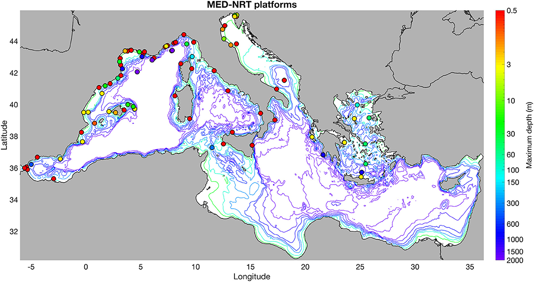
The map in Figure 1 shows the locations of the MED-NRT mooring stations in the Mediterranean Sea with the indication of their maximum sensor's depth. The map highlights the monitoring gap along the southern Mediterranean coasts which depends on the different monitoring and data sharing capacity of EU and non-EU countries (Cappelletto et al., 2021). Figure 2 presents the time coverage of the 90 moorings with time series longer than 1 year: both temperature and salinity measurements (green line), temperature only (blue line) or salinity only (red line). The vertical purple dashed lines indicate the time range, 2013 to present, on which the model validation has been performed.
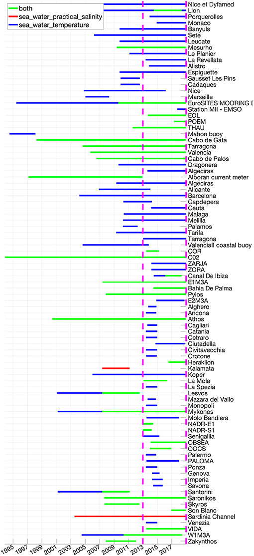
Figure 2. Time coverage of each MED-NRT mooring time series having temperature and/or salinity measurements. Only time series longer than 1 year are displayed. Purple lines indicate the time range considered for successive Cal/Val assessment.
The SOURCE models module has been implemented considering NEMO (Nucleus for European Modeling of the Ocean, Madec et al., 2019) standard output, a state-of-the-art Ocean General Circulation Model (OGCM) widely used from CMEMS Monitoring and Forecasting Centers (MFC) (Traon et al., 2017) and also by the INGV MFS model component. NEMO uses a three dimensional generalization of the Arakawa C-grid to solve the hydrodynamic primitive equations. SOURCE extracts and saves the parameters of interest in daily data sets from NEMO standard output and can handle analysis and reanalysis data. However SOURCE code could be easily adapted to read different output file formats from other OGCMs, i.e., HYCOM (https://www.hycom.org/, ROMS https://www.myroms.org/, MOM https://www.gfdl.noaa.gov/mom-ocean-model/, etc. The CF conventions (http://cfconventions.org/) were adopted for the parameter metadata description, since the naming conventions of CMEMS products and NEMO original outputs are different.
Two INGV model data sets have been used for the SOURCE setup but other CMEMS products, covering the Mediterranean Sea domain, could be integrated:
• The Mediterranean Sea reanalysis (MEDREA) (Simoncelli et al., 2019), with a horizontal resolution of 1/16th of degree on 72 levels. The MEDREA was developed at INGV within the framework of MyOcean Project and successively distributed by CMEMS until December 2020. The details about the MEDREA system are in Simoncelli et al. (2016). It covers the time period 1987–2018 and it assimilated reprocessed in situ temperature and salinity profiles and reprocessed satellite along track SLA. The QUality Information Document available at the DOI landing page reports the extensive validation and verification analysis results that annexed the product at the CMEMS web-catalog.
• The Mediterranean Sea analysis (MFS16) (Oddo et al., 2014; Clementi et al., 2016, 2017), with a horizontal resolution of 1/16th of degree on 72 levels. MFS16 has been distributed through The CMEMS Phase I (Traon et al., 2017) until December 2017 and maintained operational at INGV. It covers the time period 2013-present and it assimilates NRT in situ temperature and salinity profiles and NRT satellite along track SLA. The QUality Information Document is also available at the DOI landing page. The MFS system routine evaluation is also available at https://medforecast.bo.ingv.it/ecmwf-mfs-evaluation/.
Both INGV models have been extensively validated before their dissemination through the Copernicus Marine Service with in situ temperature and salinity profiles, satellite SST and SLA, that are semi-independent observations. The proposed SOURCE validation with independent observations from moorings is considered complementary, but also quite demanding for regional OGCMs, due to the high frequency of observations and their predominant location in the coastal region, which is characterized by a larger variability than the open ocean. SOURCE is also crucial to calibrate models, especially in the areas under the influence of rivers outflow.
3. Methods: SOURCE Implementation
The SOURCE utility is written in Python, an interpreted programming language frequently adopted in the last decade because it is versatile, ease-to-use and fast to develop. SOURCE has been developed and maintained as a module and it uses several Python modules, such as:
1. Vectorized numerical data analysis (numPy, sciPy, ObsPy, and pandas);
2. Machine learning tools (scikit-learn);
3. Hierarchical data storage (NetCDF-4) (HDF-5 extension);
4. Relational metadata storage using Structured Query Language (SQL) as management system.
Compiled programs are fast but run only on the architecture they are built for (Wes, 2012), while interpreted languages are portable but slow, lacking in optimization. Point-wise operation in arrays has to be vectorized in order to reach speed similar to compiled languages. In fact, arrays allow one to express batch operations on data without the use of for loops (Wes, 2012) and arithmetic operations on equal-size arrays can be conducted element-wise. For this reason SOURCE numerical equations went through element-wise conversion and vectorization. The code development has been carried out using git, a distributed version control system, which allows to track and disseminate all new builds, releases, and bug fixes. SOURCE is released for public use in the ZENODO platform (http://doi.org/10.5281/zenodo.5008245; Oliveri and Simoncelli, 2021) with a Creative Commons CC-BY-SA-NC license. For the software usage details, please refer to the user guide that is included in the ZENODO software distribution as the file README.md. The general SOURCE flow chart is presented in Figure 3. SOURCE is composed of three modules:
1. The observations module that manages pre- and re- processing of in situ data and builds the metadata SQL database;
2. The models module that manages model data spatial and temporal extraction and aggregation at the observed locations;
3. The Cal/Val module that assesses model quality vs. observations.
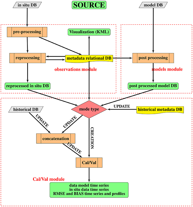
Figure 3. Flow chart of SOURCE functioning structure. The red dashed rectangles represent the three different modules. Gray parallelograms are inputs, brown rectangles are internal operations, green ellipses are outputs, yellow prints are metadata DB or logging, and orange double rectangles are the main routines. The red rhombus represents the choice between CREATION or UPDATE mode.
SOURCE uses a mixed approach for data and metadata management. The metadata information is stored in a relational SQL database, one of the most used Relational DataBase Management System (RDBMS), whose advantages are: flexibility, stability, accessibility, and management capabilities. However, these kind of database presents limitations also when dealing with Big Data. Scientific data are often organized in unstructured or hierarchical formats that are very memory demanding and maintaining them in relational structures is critical. For this reason, the data are stored in NetCDF-4, a Hierarchical Data Format 5 (HDF5) extension. Any data modification to the original data set produced by the software is stored separately to keep track of all of the changes, while all (sub-) modules and functions provide logging outputs for inspection and debugging.
SOURCE offers two different processing modes:
• The CREATION mode produces a new data collection executing all the procedures, creating from scratch metadata, data, and statistics;
• The UPDATE mode extends in time an existing data collection, integrating additional data, and metadata.
In CREATION mode, the measurements are analyzed and collated to the corresponding time series through metadata inspection. The computed statistics per platform and per parameter, such as mean, standard deviation and data density distribution are used to QC the time series and detect probable quality issues. In UPDATE mode, the new records are validated against the existing statistics. When the user wants to renovate the data collection characterization (such as statistics), SOURCE must be re-run in CREATION mode.
3.1. Observations Module
The SOURCE observations module, designed to deal with observation-based data, is composed by three sub-modules, pre processing, re-processing and production. It aggregates each mooring time series by time and depth level, it reprocesses the data and produces a quality checked database divided by ocean variable (see SOURCE flow chart in Figure 3). After downloading, the MED-NRT data are first pre processed to match SOURCE format prerequisites by selecting the space-time limits, the instruments, the variables and the desired QFs to apply. This is done through the definition of corresponding desired values in pre-processing tool. Metadata information is stored using the relational DB, while the raw time series are divided by parameter and stored in NetCDF format. The data are then re-processed by aggregating depth levels, removing duplicates and reordering record coordinate (time). Successively the data are quality controlled (QCed) maintaining the original sampling. The reprocessed and QCed data go through production in which the raw and the reprocessed data sets are saved and the time averaged data sets are created. If the process is in UPDATE mode, the metadatabase is updated to the extended collection and the QC analysis is done considering the time series characterization previously created. The reprocessed data set is finally concatenated to the existing one.
3.1.1. Pre-processing Sub-module
The MED-NRT data have to be pre-processed and re-formatted in the SOURCE internal NetCDF format in order to be correctly analyzed. To run the pre-processing procedures the user must define:
• Database directory;
• Input parameters to process (i.e., sea temperature and salinity), given as NetCDF CF conventions standard_name attributes;
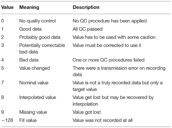
• sel_QF parameter which selects the QFs to apply (i.e., 1 for good data, 1 and 2 for both good and probably good data);
• Time range limits;
• Latitude and longitude limits;
• Platform type (i.e. “fixed platforms” devices in this SOURCE first implementation).
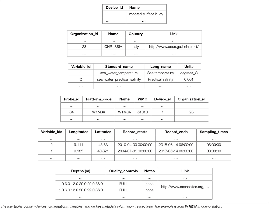
The sub-module manages the creation of the metadatabase composed of four tables: platform types, data originators, parameters, and stations. The input data set is stored in a per-parameter and a per-platform database. Each database contains the corresponding platform metadata information. Table 1 is an example of the relational metadatabase. The platform table contains:
• Platform information: unique identifier (ID), platform_code, device type ID, data originator ID, variable IDs (relations with the other tables of the database), and web link;
• Data record information: averaged latitude and longitude positions over time dimension, start and end dates, median of the sampling time, standard depth levels array, and QC type.
Let P be a platform and ϕ = ϕ(t, z′) a time series of a stored parameter where t and z′ represent time and depth coordinates, respectively. Data are stored in a matrix where rows are time and columns are depth levels. Two ancillary variables are defined: is the processed parameter and is the associated QF, as defined in Table 2.
A mooring data set is split into multiple NetCDF files if the quantity of data acquired is large (i.e., one file per recording year) or if the platform_code changes or the mooring time series presents a varying depth coordinate due to a sensor replacement. In the latest case, the data before and after the change are considered as different time series and are stored in different files. SOURCE aggregates all platform data having the same platform_code or all data having a similar platform_code string (a common case-insensitive sub-string of more than four characters) which locates within a radial distance of 2, 500m. In case of a varying depth coordinate, SOURCE handles vertical oscillations smaller than 0.5m or up to 5% increment from one depth level to another by averaging the depths. Any largest variation determines the generation of a new time series on a diverse depth level. SOURCE puts in increasing order the image of the time-varying depth function depth(t, z′), whose values are and C1, …, Cn are their multiplicities. SOURCE groups into disjoint subsets N1, …, Nm such that, if :
Then it computes a weighted average of by defining the new depth values d1, …, dm as it follows:
The final depth levels for ϕ are the subset out_depth(z) = {d1, …, dk} of {d1, …, dm}, discarding values above the sea surface and depth levels with very few associated ϕ measurements (less than 1% of total). Finally, the depth levels out_depth(z) are written in the metadatabase.
In the last phase of the pre-processing, platform data are gathered by parameter and the QF filer sel_QF is applied. In particular, the pre-processed variable is defined equal to if sel_QF, and fill_value (= 1020) otherwise. If the quality control variable ϕQF is not present, is set equal to 1 and ϕPP is defined equal to ϕ everywhere.
3.1.2. Re-processing Sub-module
The pre-processed data and metadata go through the re-processing routines which handle:
1. The record coordinate correction;
2. The depth levels aggregation;
3. The data analysis and quality control;
4. The production of raw, quality controlled, and time averaged output databases.
SOURCE uses the metadatabase, which stores for each mooring and for each parameter ϕPP the corresponding out_depth(z), to define the Depth Aggregated field ϕDA = ϕDA(t, z):
where and:
An example of depth aggregation is shown as Figure 4 for DYFAMED station: Figure 4A shows the pre-processed temperature time series along with the first two indices of the depth dimension and Figure 4B shows the depth aggregated time series on the basis of computed standard depth levels. Prior to July 10, 2014 there exist two overlapping time series associated with the same index of depth. The depth aggregated time series (Figure 4B) underline that after this date, only one time series remained at a different depth value as before. Two sensors were probably calibrated or replaced and shifted vertically.
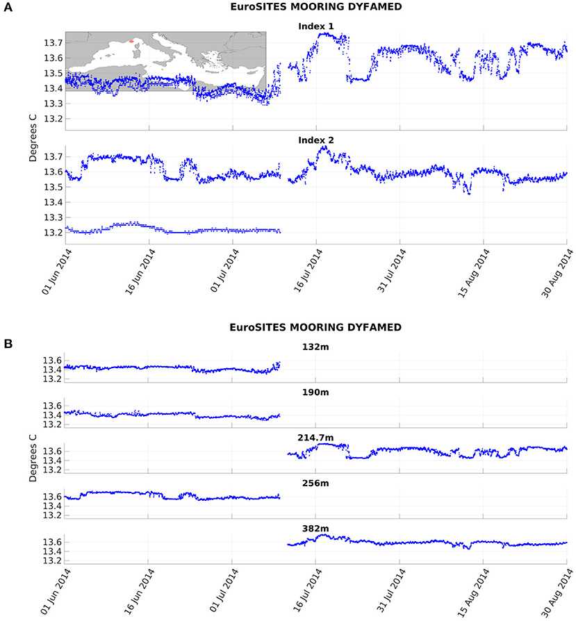
Figure 4. Example of data depth aggregation at the DYFAMED mooring in 2014: (A) temperature data at index 1 and index 2; (B) temperature data at the corresponding depths.
The time series are then checked for duplicates and monotonicity. The record coordinate (time) is rearranged to make it monotonically increasing and the duplicated records are analyzed. In case of multiple data segments, the data with the lowest sampling frequency, the lowest precision and the fewest depth levels are automatically excluded. The remaining duplicates with matching time and depth are averaged.
3.1.3. Quality Control
The data distributed by marine data infrastructures might contain undetected data anomalies, bad data flagged as “good” or “probably good.” In particular, the use of NRT data sets might include data anomalies due to undetected electronic spikes, unit errors, out of range errors, stuck values or other unpredictable outliers. The implementation of a secondary QC process, consistent between the different time series managed by different data providers, aims at applying several additional automated QC tests and statistically characterizing each mooring time series in order to detect and flag poor quality or less probable measurements and exclude them from the successive production phase.
SOURCE users can select the QC tests assigning the input parameter J:
• if J = −1 no additional QC is performed, the aggregated data are used directly in production phase as they are;
• if J = 0 the gross QC is applied, which includes out of range, electronic spikes, measure unit errors and stuck values test;
• if J = 1 the statistical QC is applied after the gross QC to detect statistical outliers
• if J > 1 the statistical QC is executed a number of J iterations.
When J = 0 a gross QC is performed following the operational QARTOD manual (U.S. Integrated Ocean Observing System, 2020) indications. Three consequent checks are executed and each check creates an associated QF and only measurements that satisfy all three tests are used in the successive processing steps:
1. RANGE CHECK: defines the global range from a minimum value ϕMIN to a maximum value ϕMAX for a variable. Data lying out of the range are flagged as anomalies:
For this configuration in the Mediterranean sea the regional parameter limits are ϕMIN = 4°C and ϕMAX = 32°C for sea water temperature and ϕMIN = 5 PSU and ϕMAX = 41 PSU for sea water salinity.
2. SPIKE TEST: checks if the variable increases or decreases as compared with 3 neighbors around each record lying within a specified range. Considering a depth level z, if Φt, z = {ϕDA(t−3, z), …, ϕDA(t−1, z), ϕDA(t+1, z), …, ϕDA(t+3, z):ϕDA(t+j, z) ≠ fill_value}:
3. STUCK VALUE TEST: detects if the occurrence of each different value is within its 100 nearest values. Given a depth level z, ψ = ϕDA(t, z), Cψ = #{t:ϕDA(t, z) = ψ}, ψ1, …, ψ100 the 100 different values of ϕDA nearest to ψ and CΨ = {#{t:ϕDA(t, z) = ψj}} the corresponding occurrences set, ψ is a stuck value if Cψ > 100 and . Therefore:
Finally:
Two examples of gross QC output are shown in Figure 5 for OBSEA and Ponza mooring stations in which anomalous temperature values have been detected: in the first case there are (Figure 5A) temperature records multiplied by a scaling factor; in the second case (Figure 5B) a repeated stuck value of 20°C appears.
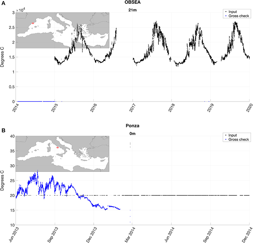
Figure 5. Examples of erroneous data detection for sea water temperature by gross check: (A) OBSEA station; (B) Ponza station.
When J = 1 the statistical QC is executed after the gross QC. A temporary variable ϕGOOD = ϕGOOD(t, z) is created such that:
To perform a reliable statistical outlier detection, both the seasonal and long-term components have to be removed from the time series ϕGOOD to get stationary residuals. The removal of the seasonal component is based on the calculation of the monthly mean. For each level z and for each month m ∈ {1, …, 12}, given the number Nm, z, j of all valid records t1, …, tNm, z, j of ϕGOOD(·, z) such that
the monthly mean ϕμ is:
SOURCE computes also the relative standard deviation:
The de-seasonalized time series is defined by:
for all records t such that:
The linear trend is computed by the scikit-learn machine learning module sklearn.linear_model.LinearRegression model (scikit-learn.org). The trend that fits ϕDSN(·, z, j) is , where α is the regression slope and β is the intercept. The coefficient of determination , which provides a measure of how well measurements are replicated by the linear model is also computed:
assuming zero mean value for ϕDSN(·, z, j). If , the detrended residual associated to ϕ is computed:
Otherwise, the linear de-trending is deactivated and the residual ϕDSN(·, z, j) is used instead of ϕRES(t, z, j).
SOURCE then detects and flags statistical outliers, i.e., points of low probability, by estimating the Probability Density Function (PDE). Let X = ϕRES(·, z, j) be a random variable in terms of probability, a and b two possible values for X, the PDF of X is:
where fX if the density function of X. If dx is an infinitely small interval, the probability that X is included within the range (x, x + dx) is equal to f(x)dx. SOURCE computes a real approximation of fX using the Kernel Density Estimation (KDE) available in Python's scikit-learn machine learning module. As stated in scikit-learn documentation (scikit-learn.org/stable/modules/density.html), density estimation walks the line between unsupervised learning, feature engineering and data modeling. The KDE follows a neighbor-based approach and its use results in a smooth density estimate derived from the data, working as a powerful non-parametric model of the distribution of points. In mathematical terms a kernel is a positive function K = K(x, h) controlled by the bandwidth parameter h. The bandwidth h acts as a smoothing parameter, controlling the trade-off between bias and variance in the result. A large bandwidth leads to a very smooth density distribution; a small bandwidth leads to a rough density function. Scikit-learn algorithm implements several common kernel forms (Gaussian, linear, tophat, etc.). Given a kernel form, the density estimate at a point y within a group of points x1, …, xN is given by:
Gaussian kernels with bandwidth 0.2 have been selected for the SOURCE statistical QC implementation. The direct density estimate of X (i.e., the residuals) can be time consuming, thus a set of sample values from -10 to 10, increasing by 0.1, has been used instead, considering the residuals falling between ±10°C for temperature and ±10 PSU for salinity. The probability distribution ℙ(ϕRES(·, z, j) = ϕRES(t, z, j)) is then computed from the density function, deriving each value of ϕRES(·, z, j) using the one dimensional linear interpolation from Python's scipy module.
The statistical QC procedure flags and inhibits from further use the measures whose probability of occurrence is lower than 5%:
The procedure then recomputes the mean μ and standard deviation σ.
When J > 1 the statistical QC is re-executed J times, subtracting the seasonality and trend, recomputing the PDF from the residuals, flagging the statistical outliers, witholding them from the computation of new μ and σ.
The statistics (μ, σ, and the PDF) are computed in CREATION mode only per each mooring platform for each depth aggregated parameter ϕDA and are stored in files for further use in UPDATE mode (where new NRT measurements are collated to the already present time series) until the user decides to re-run the full procedure in CREATION mode.
3.1.4. Production
At the end of re-processing, SOURCE produces three different types of output for each time series ϕ :
• ϕDA RAW data;
• ϕQC reprocessed data at the original sampling time;
• Different time averages (i.e., hourly, daily, monthly, annual) depending on the original sampling time.
The data production phase takes into account the depth aggregated field ϕDA and the corresponding quality information ϕRQF. Given the input parameter J ≥ 1, the validated time series ϕQC = ϕQC(t, z) is then created:
SOURCE's time averaging capabilities are quite flexible and sophisticated: the use of Python's pandas package allows to calculate time weighted averages from a second to a year and to manage averages where the instrument sampling interval is greater than the requested averaged frequency by less than 10%. The time averaged output can have hourly, daily, monthly and yearly frequencies.
In UPDATE mode the produced data set has to be concatenated with a historical data set generated in CREATION mode. SOURCE routines handle the update of the relational metadatabase adding new attributes such as data providers, device types, variables, platforms, sensors at different depths and updating time ranges and QFs. Finally, an additional SOURCE utility creates a Keyhole Markup Language (KML) file for mapping from the metadatabase containing all desired information in the selected region.
3.2. Models Module
The aim of the models module is to extract model time series at the observed space-time mooring locations in order to compare model output with observations. The comparison is first qualitative, through visual inspection and then quantitative, through the computation of skill scores performed in the Cal/Val sub-module. Besides the continuous validation or calibration of model results, the visual inspection of the time series allows a continuous monitoring of both the instrument calibration and the sea conditions at the mooring location.
SOURCE takes the input provided by the user in terms of location, parameter to be analyzed, time frequency and input model. The selected model outputs must reside in the SOURCE input directory or in sub-directories named after the corresponding variable standard name according to the NetCDF CF conventions and the user has to provide the metadata information from the reprocessed in situ database. SOURCE then finds the closest model grid point to each mooring location, within a certain user-defined distance, it extracts a model, named hereafter synthetic time series, and it compares the model with observations at the corresponding depths. A necessary input is the model grid information. If this is not present embedded in the model data set, the user must provide the land-sea mask separately in NetCDF format. Other input parameters are:
• Time range limits;
• Latitude and longitude horizontal limits (relocatability);
• Concatenation flag to enable or disable the gridded data sets concatenation;
• Interpolation flag to enable or disable the vertical interpolation on mooring depths;
• Maximum acceptable horizontal distance to produce model time series, expressed in kilometers, from each platform to the nearest model sea grid point.
If the concatenation option is enabled, SOURCE uses the metadatabase to create the list of mooring locations for each parameter where the synthetic time series will be extracted over the entire water column. Let P be a platform recording the parameter ϕ at the location (P_lat, P_lon) and ϕM = ϕM(t, z, y, x) the model parameter with coordinates (grid_lat, grid_lon), SOURCE computes:
where dist𝔼 is the Great Radius Earth distance:
Only if the radial distance between the mooring and the nearest sea grid point is less than the specified maximum acceptable distance, is the available model data extracted and concatenated. MFS16 and MedRea16 models have coincident grids with horizontal resolution of approximately 6.5 km and the distance between the mooring and the closest sea-grid point is always confined within the grid size distance except for six cases. Most of them range between 1 and 4 km and the largest distance is less than 9.8 km, which corresponds approximately to the diagonal of the model grid cell. All moorings have been considered for the assessment, however setting a threshold distance is important when the models have different grids and the user should carefully evaluate this aspect.
The observed and synthetic variables are then harmonized following the observations conventions. If the vertical interpolation option is enabled, the mooring depth levels (out_depth) are loaded from the metadatabase and one dimensional linear interpolation (Python's scipy) is applied. Out of bound values of interpolation are treated as follows:
• At the surface, if the observed and model depths are both shallower than 2m and the observed depth is shallower than the first model level: the synthetic time series is considered without any interpolation.
• At the bottom, if the observed depth is deeper than the model bottom depth and the latter is shallower than 700m: the synthetic time series at the model bottom level is considered if the difference between observed and model bottom depth is less than 10% of the model bottom depth; if the model bottom depth is deeper than 700m the synthetic time series at the bottom level is used if the difference between observed and model depth is less than 20% of the model depth.
Otherwise the synthetic time series is not extracted and the model validation not performed. Synthetic data are then harmonized, if necessary, to the observed data (i.e., the model potential temperature and practical salinity fields are used to produce the in situ temperature). If the concatenation option is disabled (the process may be quite time consuming), SOURCE allows to perform vertical interpolations from existing concatenated time series. This allows to avoid new concatenations in the case of new depths required by the user in the same locations. Moreover, if the user wants to analyze all the levels of the model output, SOURCE includes this option, and only concatenation will be performed. In UPDATE mode the incoming synthetic data have to be concatenated to the already existing ones; the procedure is the same as above.
3.3. Cal/Val Module
SOURCE evaluates model performance through the computation of basic skill's scores at the platform locations once the observed ϕo = ϕo(t, z) and synthetic ϕm = ϕm(t, z) data are generated. The evaluation module loads both observed and synthetic data time series and computes the class 4 metrics (Simoncelli et al., 2016) differences and absolute error, defined as follows:
where the t ∈ {1, …, Tz} are the time records in the selected period.
4. Results
SOURCE provides reprocessed time series with improved quality thanks to the application of a secondary QC procedure, consistently applied to all the available MED-NRT mooring stations. It allows to compute most accurate model skill scores through the extraction of synthetic time series and, at the same time, to get mooring site characterization and to monitor the sea condition and its variability. SOURCE output includes the reprocessed time series ϕDA and the following relative fields:
• The monthly mean (climatology) μ and standard deviation σ;
• The residuals ϕRES, i.e., the modified ϕDA by filtering out seasonality and long-term trend components;
• The long term trend computed from the de-seasonalized time series;
• The PDF fϕRES;
• The reprocessed time series with updated QF ϕRQF;
• The percentage of rejected data Rp = Rp(z, J + 1) at each QC step.
Figure 6A shows an example of monthly mean and the associated standard deviation for surface temperature at Monaco station, computed after gross check and after each of the three iterations of the recursive statistical QC. Slight variations of climatological averages and standard deviations are evident as the effect of rejected data. The corresponding time series of residuals after the subtraction of seasonal and long term components are displayed in Figure 6B after each step of the QC process, gross check and three statistical loops. The surface temperature PDF and the reprocessed time series after each iteration are shown in Figures 7A,B, respectively. Additionally, in the box of panel B the statistics of detected anomalous data are summarized: 0.83% are identified by the gross check, 1.15% from the first statistical QC loop, 0.19% and 0.06% from the second and third respectively. The statistics about the rejected data Rp = Rp(z, J + 1) (flagged as “bad,” QF = 4) at each QC step are very useful and some sensitivity tests are advisable to tune the QC to the user and application purpose. The results of MED-NRT mooring data reprocessing are summarized in Table 3, which shows the mean percentage of rejected measurements at each QC step computed from all reprocessed stations in Figure 2. The spike test is detecting the highest percentage of anomalous data(0.63% for temperature and 0.86% for salinity) among the gross check tests, higher than range and stuck value tests. The first statistical QC loop captures the largest percentages of anomalous data: 1.81% of temperature and 3.18% of salinity measurements.
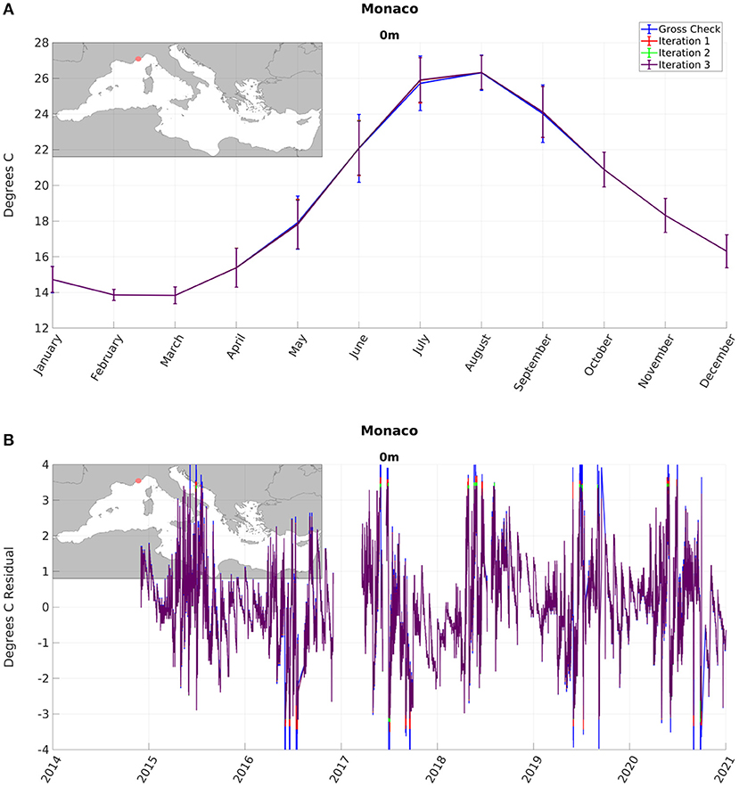
Figure 6. Surface temperature at Monaco station: (A) monthly climatology and standard deviation; (B) residuals. The lines show the input data (passed gross QC) to the recursive statistical QC and the output of its three iterations.
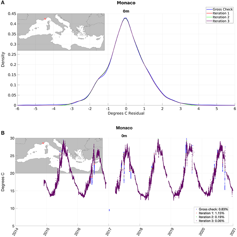
Figure 7. Surface temperature at Monaco station: (A) Probability Density Function (PDF) computed from residuals; (B) statistical QC progression. The lines show the input data to the recursive statistical QC and the output of the 3 applied iterations.

Table 3. Mean percentages of detected anomalies obtained from all mooring time series in the various reprocessing steps.
A summary of mooring statistical characterization of salinity at Tarragona station obtained from SOURCE reprocessing is displayed in Figure 8. Tarragona station is located in front of the Ebro River (Spain), thus the salinity at 3m depth is influenced by the river freshwater outflow, ranging from about 37 to 38.5 PSU. The low salinity values are thus within the mooring site variability and consequently they have not been flagged by the recursive statistical QC.

Figure 8. Mooring site characterization of salinity at 3 m depth: (A) reprocessed time series and trend line; (B) monthly climatology and standard deviation; (C) de-seasonalized and detrended time series of residuals; (D) Probability Density Function (PDF) of residuals.
Figure 9 shows the daily mean temperature and salinity time series at Monaco and Tarragona stations. The blue dotted line represents the average computed from the MED-NRT data set before SOURCE reprocessing, while the red line represents the average computed from reprocessed data that passed successfully both gross check and recursive statistical QC.
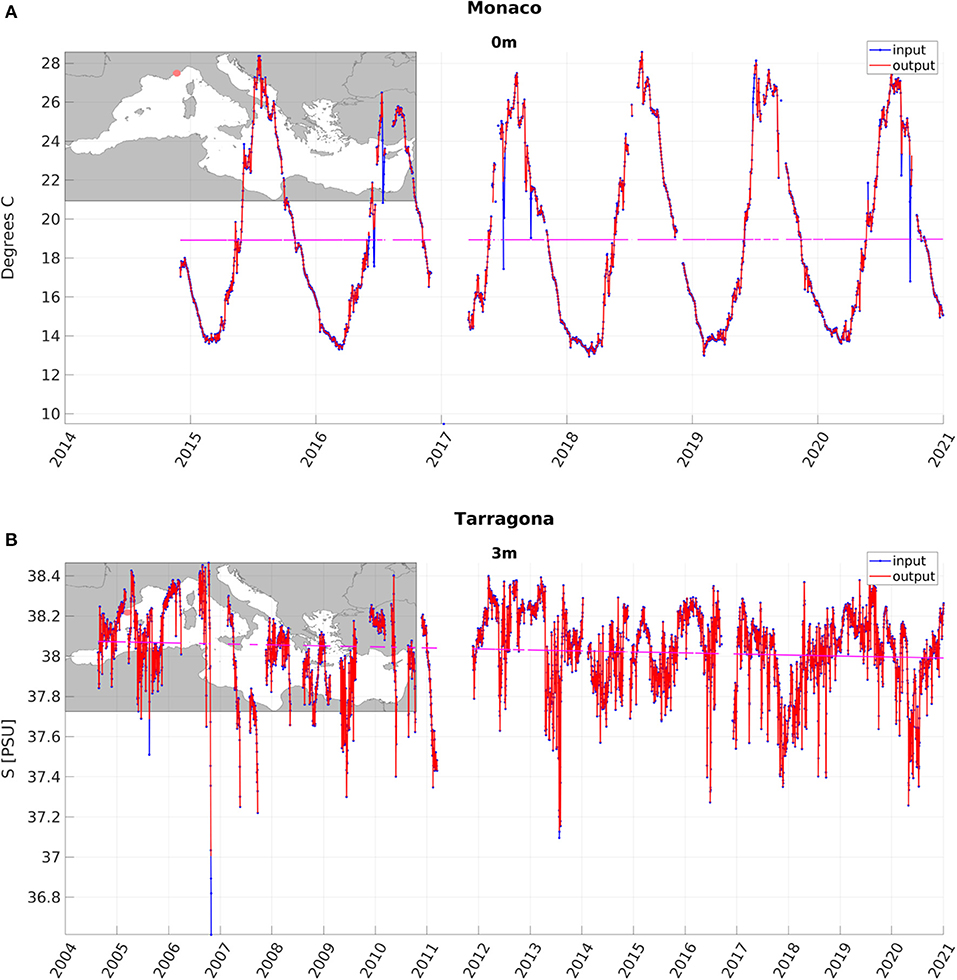
Figure 9. Daily averages computed without (black line) executing and after applying the SOURCE data reprocessing (gross QC and recursive statistical QC): (A) surface temperature at Monaco station; (B) salinity at Tarragona station at 3 m depth.
SOURCE makes it possible to validate multiple models within a selected sea region, the Mediterranean Sea in this case, through the computation of basic skill scores which consider the reprocessed mooring time series obtained from the MED-NRT data set delivered by CMEMS In Situ TAC. The purpose of this SOURCE configuration is the validation of INGV model MFS16 daily analysis in CREATION mode and the validation of MedRea16 reanalysis over the covered time period prior to 2018. There are multiple options to visualize results from SOURCE models and Cal/Val modules at each mooring location such as (see Figure 10) the histogram of differences between observations and models (bias) or the scatter plot of observed vs. model values, which provides also correlation estimates for a selected parameter. This kind of visualization allows to assess multiple models or different model implementations (calibration). Figure 10A presents daily mean surface temperature time series of MedRea16 and MFS16 models vs. observations over the time period 2013-2018 at Monaco station, together with the computed skill scores. MFS16 is matching quite well the observed temperature (MED-NRT), while MedRea16 exhibits frequently lower temperature values than observed. The RMSE and bias are reflecting models behavior with lower values (0.35 and 0.04°C) from MFS16 than (0.67° and −0.63°C) MedRea16. The histogram in Figure 10B shows the distribution of the temperature differences between the models and observations: MedRea16 differences (red bars) are shifted toward negative values that determine a noticeable negative mean bias (−0.63°C) while MFS16 distribution (blue bars) is more centered around zero with a mean bias almost nil (0.04°C). The scatter plot in Figure 10C is another way to display the observed vs. model temperatures and the regression lines that give indication of their correlation.
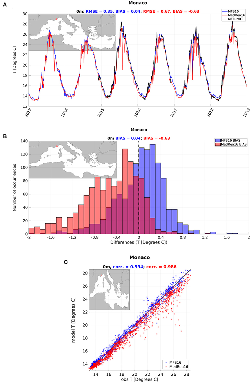
Figure 10. Surface temperature validation of MedRea16 and MFS16 models at Monaco station: (A) synthetic and observed time series; (B) histogram of differences between model and observated temperature; (C) scatter plot of observed vs. model temperature.
SOURCE provides information at all mooring locations and these could be summarized and displayed at basin scale either from observations to present the computed statistics (i.e., climatologies or trends) or model skill scores. As an example, Figure 11 shows a comparison between the MED-NRT platform climatologies in the layer 0–3 m (colored dots near the coast) and the first depth level (approx. 1.4 m) of MedRea16 monthly climatology (distributed colored fields) in September (Figure 11A) and July (Figure 11B), computed over the time period 2013–2018. The SOURCE Cal/Val module results from all MED-NRT platforms can be used as quality evaluation of model temperature or salinity in the selected domain, the Mediterranean Basin in this case, even if the available mooring platforms are located mainly along the northern coasts. In fact, this kind of visualization can provide an overview of the performance of the model in a certain depth level from all moorings, indicating where the model has the best or the worst performance. This is an important tool to validate and calibrate models in the coastal region where rivers influence both temperature and salinity fields, as the case of Tarragona station in Figure 8, influenced by the Ebro river outflow.
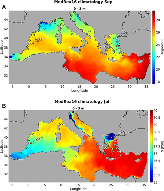
Figure 11. Comparison between monthly climatologies from MED-NRT mooring time series in the layer 0–3 m (colored dots) and the surface fields of MedRea16 (approx. 1.4 m) computed in the time period 2013–2018: (A) temperature in September; (B) salinity in July. Only time series longer than 1 year are displayed.
Figure 12A shows the map of the estimated temperature absolute errors of MedRea16 model over the time period 2013-2018 in the surface layer 0–3 m, computed with reprocessed time series (gross and recursive statistical QC) from the available MED-NRT platforms. This functionality provides a broad view of model behavior, giving indication of the locations where the model performance is good or bad for further inspection and solution implementation. Figure 12B provides the difference of absolute errors estimated from all good or probably good (QF = 1,2) input data and from reprocessed data, which demonstrates the overall not negligible impact of SOURCE secondary QC on model skill score. Figure 12C presents the effect of the recursive statistical QC from absolute errors differences before and after its execution. The differences in Figure 12B are larger than in Figure 12C, reaching about 1°C in several stations, due to a larger impact of filtering gross errors than statistical outliers on model skill score.
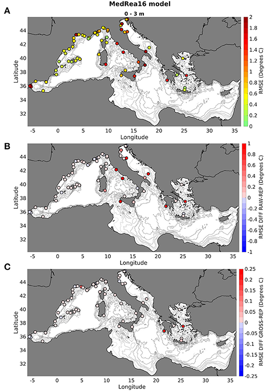
Figure 12. Temperature RMSE of MedRea16 model computed at MED-NRT mooring locations over the time period 2013–2018 in the surface layer 0–3 m: (A) RMSE obtained after mooring data reprocessing (gross QC and recursive statistical QC); (B) differences between RMSE using raw data and reprocessed data; (C) differences between RMSE using data after gross QC as reprocessed data.
5. Conclusions
SOURCE utility has been developed to be a relocatable and flexible software for web-based application that performs validation and calibration of ocean model data through inter-comparison with reprocessed in situ observations. The model validation is performed at the observation location through the computation of basic metrics. The observed data go through: a pre-processing tool for data and metadata ingestion and integration in metadatabase and database and a reprocessing tool which performs gross check and recursive statistical QC for the highest data quality and a most accurate computation of derived model skill scores.
Observations to be utilized in SOURCE can be accessed through existing marine data portals (i.e., CMEMS, SeaDataNet, EMODnet, World Ocean Database, EMSO). In this case SOURCE implementation considers NRT mooring data (fixed platforms) from the CMEMS In Situ TAC and two INGV model products, daily analysis (Clementi et al., 2016) and reanalysis (Simoncelli et al., 2019) over the Mediterranean Sea domain.
The SOURCE secondary and recursive QC procedures of mooring time series permits one to characterize the ocean variability at a mooring site to monitor the ocean conditions. Moreover a double NRT check is possible through the continuous visual inspection of either anomalous measurements which can uncover sensor failure or out of calibration observations, model drifts or inability to resolve high frequency processes recorded by moorings, especially in the coastal area where the ocean variability is the largest. Models can thus be calibrated using SOURCE to intercompare different model versions including for example new parameterizations.
The SOURCE monitoring capability and mooring site characterization rely on basic statistical analyses of in-situ data, complemented by new Machine Learning (ML) functionalities, to derive monthly climatologies and standard deviations, trends and PDFs of residuals obtained from de-seasonalization and de-trending of reprocessed time series. SOURCE provides also daily, monthly, and annual data averages.
This first and basic SOURCE implementation is shared with the community as a starting tool having a high development potential. Its results are already accessible at the website http://calval.bo.ingv.it/ and the next step will be the renovation of the website design and functionalities in order to show all the SOURCE output typologies for the users' consultation.
Further SOURCE development has already started to integrate mooring data from SeaDataNet and EMSO marine data infrastructures, important for deep-sea monitoring and model development in the challenging deep ocean. Another data source to consider is the World Ocean Database (WoDB). Data integration from multiple sources is challenging due to the metadata integration and duplicates management. Another improvement will be the inclusion of additional parameters such as sea level, currents and met-ocean variables (i.e., air temperature, wind), completing the assessment of the main ocean model output or atmospheric forcing variables. Additional model products from CMEMS will be included, either from global or regional ocean circulation models, to assess the consistency among different model solutions and derive ensemble model estimates. Satellite gridded products can also be integrated for model Cal/Val and ocean monitoring. New early warning system applications, such as marine heatwaves detection, based on ocean forecasting will be also considered.
Data Availability Statement
Publicly available datasets were analyzed in this study. This data can be found here: Mediterranean Sea - near real-time (NRT) in situ quality controlled observations are available at https://resources.marine.copernicus.eu/?option=com_csw&view=details&product_id=INSITU_MED_NRT_OBSERVATIONS_013_035. Copernicus Marine In Situ Tac Data Management Team (2021). Product User Manual for multiparameter Copernicus In Situ TAC (PUM). https://doi.org/10.13155/43494. Copernicus Marine in situ TAC (2021). Copernicus Marine In Situ TAC quality information document for Near Real Time In Situ products (QUID and SQO). https://doi.org/10.13155/75807 MedRea16 Mediterranean Physics Reanalysis is available upon request at https://doi.org/10.25423/MEDSEA_REANALYSIS_PHYS_006_004. The Mediterranean Physics Analysis data 2013–2017 are available upon request at https://doi.org/10.25423/MEDSEA_ANALYSIS_FORECAST_PHYS_006_00. Recent data are available upon request to the corresponding author.
Author Contributions
PO devised SOURCE code under the supervision of SS, wrote sections 2 and 3 of the manuscript, and produced the figures and tables. SS wrote the rest of the manuscript. PD helped the transition between the old procedures and SOURCE. DD supported the code development. CF, AG, and GM reviewed the manuscript. GM coordinates the INGV funding project. All authors contributed to the article and approved the submitted version.
Funding
This work has been co-funded by the Italian RITMARE Flagship Project and the INGV internal project Relocatable integrated Cal/Val system for sea observations reprocessing and ocean models evaluation (project code 9999.526 - RL2019).
Conflict of Interest
The authors declare that the research was conducted in the absence of any commercial or financial relationships that could be construed as a potential conflict of interest.
Publisher's Note
All claims expressed in this article are solely those of the authors and do not necessarily represent those of their affiliated organizations, or those of the publisher, the editors and the reviewers. Any product that may be evaluated in this article, or claim that may be made by its manufacturer, is not guaranteed or endorsed by the publisher.
Acknowledgments
We thank Alessandro Grandi and Emanuela Clementi, former colleagues and now at Centro Euro-Mediterraneo per i Cambiamenti Climatici (CMCC), for their advise that helped to design the new SOURCE utility. This study has been conducted using E.U. Copernicus Marine Service Information. We thank also William Emery from University of Colorado Boulder for his advices.
References
Bailey, K., Steinberg, C., Davies, C., Galibert, G., Hidas, M., McManus, M. A., et al. (2019). Coastal mooring observing networks and their data products: recommendations for the next decade. Front. Mar. Sci. 6:180. doi: 10.3389/fmars.2019.00180
Borg, A., Husted, B. P., and Nja, O. (2014). The concept of validation of numerical models for consequence analysis. Reliabil. Eng. Syst. Saf. 25, 36–45. doi: 10.1016/j.ress.2013.09.009
Bushnell, M., Waldmann, C., Seitz, S., Buckley, E., Tamburri, M., Hermes, J., et al. (2019). Quality assurance of oceanographic observations: standards and guidance adopted by an international partnership. Front. Mar. Sci. 6:706. doi: 10.3389/fmars.2019.00706
Capet, A., Fernandez, V., She, J., Dabrowski, T., Umgiesser, G., Staneva, J., et al. (2020). Operational modeling capacity in european seas, an eurogoos perspective and reccomendations for improvement. Front. Mar. Sci. 7:129. doi: 10.3389/fmars.2020.00129
Cappelletto, M., Santoleri, R., Evangelista, L., Galgani, F., Garcés, E., Giorgetti, A., et al. (2021). The Mediterranean Sea we want. Ocean Coast. Res. 69, 17–19. doi: 10.1590/2675-2824069.21019mc
Clementi, E., Oddo, P., Drudi, M., Pinardi, N., Korres, G., and Grandi, A. (2017). Coupling hydrodynamic and wave models: first step and sensitivity experiments in the mediterranean sea. Ocean Dyn. 67, 1293–1312. doi: 10.1007/s10236-017-1087-7
Clementi, E., Pistoia, J., Fratianni, C., Delrosso, D., Grandi, A., Drudi, M., et al. (2016). Mediterranean Sea Analysis and Forecast (CMEMS MED-Currents 2013–2017) [Data set]. Copernicus Monitoring Environment Marine Service (CMEMS). doi: 10.25423/MEDSEA_ANALYSIS_FORECAST_PHYS_006_001
Copernicus Marine In Situ Tac Data Management Team (2019). Product User Manual for Copernicus in situ TAC (PUM). Technical document, Copernicus Marine Environment (CMEMS).
Cowley, R., Killick, R. E., Boyer, T., Gouretski, V., Reseghetti, F., Kizu, S., et al. (2021). International quality-controlled ocean database (IQUOD) v0.1: the temperature uncertainty specification. Front. Mar. Sci. 8:607. doi: 10.3389/fmars.2021.689695
Crosnier, L., and Le Provost, C. (2007). Inter-comparing five forecast operational systems in the north Atlantic and Mediterranean basins: the mersea-strand1 methodology. J. Mar. Syst. 65, 354–375. doi: 10.1016/j.jmarsys.2005.01.003
Davidson, F., Alvera-Azcarate, A., Barth, A., Brassington, G. B., Chassignet, E. P., Clementi, E., et al. (2019). Synergies in operational oceanography: the intrinsic need for sustained ocean observations. Front. Mar. Sci. 6:450. doi: 10.3389/fmars.2019.00450
Hernandez, F., Blockley, E., Brassington, G. B., Davidson, F., Divakaran, P., Drevillon, M., et al. (2015). Recent progress in performance evaluations and near real-time assessment of operational ocean products. J. Oper. Oceanogr. 8(Suppl 2):s221–s238. doi: 10.1080/1755876X.2015.1050282
Le Traon, P. Y., Reppucci, A., Alvarez Fanjul, E., Aouf, L., Behrens, A., Belmonte, M., et al. (2019). From observation to information and users: the copernicus marine service perspective. Front. Mar. Sci. 6:234. doi: 10.3389/fmars.2019.00234
Madec, G., Bourdalle-Badie, R., Chanut, J., Clementi, E., Coward, A., Ethe, C., et al. (2019). NEMO Ocean Engine. Institut Pierre-Simon Laplace (IPSL).
Nowak, K., Nielsen, L. H., Ioannidis, P., and Alexandros, T. (2016). Zenodo, a Free and Open Platform for Preserving and Sharing Research Output. Florida, FL: Zenodo. doi: 10.5281/zenodo.51902
Oddo, P., Bonaduce, A., Pinardi, N., and Guarnieri, A. (2014). Sensitivity of the mediterranean sea level to atmospheric pressure and free surface elevation numerical formulation in nemo. Geosci. Model Dev. 7, 3001–3015. doi: 10.5194/gmd-7-3001-2014
Ryabinin, V., Barbiere, J., Haugan, P., Kullenberg, G., Smith, N., McLean, C., et al. (2019). The UN decade of ocean science for sustainable development. Front. Mar. Sci. 6:470. doi: 10.3389/fmars.2019.00470
Simoncelli, S., Fratianni, C., Pinardi, N., Grandi, A., Drudi, M., Oddo, P., et al. (2019). Mediterranean Sea Physical Reanalysis (CMEMS MED-Physics) (No. 1) [Data set]. Copernicus Monitoring Environment Marine Service (CMEMS). doi: 10.25423/MEDSEA_REANALYSIS_PHYS_006_004
Simoncelli, S., Manzella, G. M., Storto, A., Pisano, A., Lipizer, M., Barth, A., et al. (2021). “Chapter 4: A collaborative framework among data producers, managers, and users,” in Ocean Science Data, eds G. Manzella and A. Novellino (Amsterdam: Elsevier), 197–280.
Simoncelli, S., Masina, S., Axell, L., Salon, S., Cossarini, G., Laurent, B., et al. (2016). Myocean regional reanalyses: overview of reanalysis systems and main results. Mercator Ocean J. 54, 43–64.
Tonani, M., Nilsson, J., Lyubartsev, V., Grandi, A., Aydogdu, A., Azzopardi, J., et al. (2012). Operational evaluation of the Mediterranean monitoring and forecasting centre products: implementation and results. Ocean Sci. Discuss. 9, 1813–1851. doi: 10.5194/osd-9-1813-2012
Traon, P. L., Ali, A., Fanjul, E. A., Aouf, L., Axell, L., Aznar, R., et al. (2017). The copernicus marine environmental monitoring service: main scientific achievements and future prospects. Spcl. Issue Mercator Ocean J. 56, 56–59.
US Integrated Ocean Observing System (2020). Manual for Real-Time Quality Control of In-situ Temperature and Salinity Data Version 2.1: A Guide to Quality Control and Quality Assurance of In-situ Temperature and Salinity Observations. U.S. Department of Commerce, National Oceanic and Atmospheric Administration, National Ocean Service, Integrated Ocean Observing System, Silver Spring, MD.
Keywords: ocean observation, Cal/Val, reprocessing, Python, NetCDF, ocean best practices, OGCM evaluation, quality controls
Citation: Oliveri P, Simoncelli S, Di Pietro P, Fratianni C, Mattia G, Delrosso D and Guarnieri A (2022) SOURCE: Sea Observations Utility for Reprocessing, Calibration and Evaluation. Front. Mar. Sci. 8:750387. doi: 10.3389/fmars.2021.750387
Received: 30 July 2021; Accepted: 14 December 2021;
Published: 27 January 2022.
Edited by:
Joanna Staneva, Institute of Coastal Systems Helmholtz Centre Hereon, GermanyReviewed by:
Byoung-Ju Choi, Chonnam National University, South KoreaJaume Piera, Institute of Marine Sciences, Spanish National Research Council (CSIC), Spain
Copyright © 2022 Oliveri, Simoncelli, Di Pietro, Fratianni, Mattia, Delrosso and Guarnieri. This is an open-access article distributed under the terms of the Creative Commons Attribution License (CC BY). The use, distribution or reproduction in other forums is permitted, provided the original author(s) and the copyright owner(s) are credited and that the original publication in this journal is cited, in accordance with accepted academic practice. No use, distribution or reproduction is permitted which does not comply with these terms.
*Correspondence: Paolo Oliveri, cGFvbG8ub2xpdmVyaUBpbmd2Lml0
 Paolo Oliveri
 Simona Simoncelli
 Pierluigi Di Pietro
 Claudia Fratianni
 Damiano Delrosso
 Antonio Guarnieri