 Piero L. F. Mazzini
 Cassia Pianca
94% of researchers rate our articles as excellent or good
Learn more about the work of our research integrity team to safeguard the quality of each article we publish.
Find out more
ORIGINAL RESEARCH article
Front. Mar. Sci., 07 January 2022
Sec. Coastal Ocean Processes
Volume 8 - 2021 | https://doi.org/10.3389/fmars.2021.750265
Prolonged events of anomalously warm sea water temperature, or marine heatwaves (MHWs), have major detrimental effects to marine ecosystems and the world's economy. While frequency, duration and intensity of MHWs have been observed to increase in the global oceans, little is known about their potential occurrence and variability in estuarine systems due to limited data in these environments. In the present study we analyzed a novel data set with over three decades of continuous in situ temperature records to investigate MHWs in the largest and most productive estuary in the US: the Chesapeake Bay. MHWs occurred on average twice per year and lasted 11 days, resulting in 22 MHW days per year in the bay. Average intensities of MHWs were 3°C, with maximum peaks varying between 6 and 8°C, and yearly cumulative intensities of 72°C × days on average. Large co-occurrence of MHW events was observed between different regions of the bay (50–65%), and also between Chesapeake Bay and the Mid-Atlantic Bight (40–50%). These large co-occurrences, with relatively short lags (2–5 days), suggest that coherent large-scale air-sea heat flux is the dominant driver of MHWs in this region. MHWs were also linked to large-scale climate modes of variability: enhancement of MHW days in the Upper Bay were associated with the positive phase of Niño 1+2, while enhancement and suppression of MHW days in both the Mid and Lower Bay were associated with positive and negative phases of North Atlantic Oscillation, respectively. Finally, as a result of long-term warming of the Chesapeake Bay, significant trends were detected for MHW frequency, MHW days and yearly cumulative intensity. If these trends persist, by the end of the century the Chesapeake Bay will reach a semi-permanent MHW state, when extreme temperatures will be present over half of the year, and thus could have devastating impacts to the bay ecosystem, exacerbating eutrophication, increasing the severity of hypoxic events, killing benthic communities, causing shifts in species composition and decline in important commercial fishery species. Improving our basic understanding of MHWs in estuarine regions is necessary for their future predictability and to guide management decisions in these valuable environments.
Analogous to the well studied heatwaves in the atmosphere (e.g., Perkins, 2015), prolonged anomalously warm events also occur in the ocean, and are referred to as Marine Heatwaves (MHWs). Coined by Pearce et al. (2011), these extreme events have only recently become targeted by the scientific community (Hobday et al., 2018) despite their major ecological and economic impacts (Oliver, 2021). For instance, notable MHW events have been associated with record-breaking harmful algal blooms (McCabe et al., 2016; Gobler, 2020; Trainer et al., 2020), have led to global-scale coral bleaching (Hughes et al., 2017; Eakin et al., 2019), geographical species shifts and changes in species composition (Ehlers et al., 2008; Cavole et al., 2016; Sanford et al., 2019), mortality of kelps, submerged aquatic vegetation (SAV), invertebrates (Moore and Jarvis, 2008; Garrabou et al., 2009; Marb and Duarte, 2010; Fraser et al., 2014; Thomson et al., 2015; Wernberg et al., 2016; Shields et al., 2018, 2019; Seuront et al., 2019; Thomsen et al., 2019; Filbee-Dexter et al., 2020; Aoki et al., 2021; Johnson et al., 2021), and impacted commercial fisheries and aquaculture (Mills et al., 2013; Caputi et al., 2016; Oliver et al., 2017; Jacox, 2019). While these acute events have drastic immediate consequences, MHWs can also have long lasting detrimental effects to the marine ecosystem (Pansch et al., 2018; Oliver et al., 2019; Smale et al., 2019).
Significant advances in the characterization of MHWs have been accomplished at global scales, primarily due to the availability of sea surface temperature (SST) data obtained through satellite remote sensing (Holbrook et al., 2019). Both the frequency, duration and intensity of MHWs have been observed to increase in the global oceans over the past decades (Oliver et al., 2018), and due to long-term ocean warming under climate change, this trend is expected to further increase in the future (Frölicher and Laufkötter, 2018; Oliver et al., 2019). While the satellite data products used in those studies can resolve open ocean and shelf scales (e.g., Marin et al., 2021), because of their relative coarse resolution (~25 km) they typically fail to resolve most estuarine systems, which are characterized by having complex shorelines and reduced spatial scales.
Estuaries occupy less than 1% of the earth's surface area, but are one of the most productive marine ecosystems in our planet, and home to roughly 60% of the human population, that reside along the shorelines and in the vicinity of these crucial environments. Furthermore, estuaries serve as nursery habitats for a number of marine species and support major economic activities including aquaculture, fishing and tourism, providing several ecosystem services and benefits to our society. While warming trends have been detected in a number of estuaries across the globe (e.g., Ashizawa and Cole, 1994; Najjar et al., 2010; Seekell and Pace, 2011; Ding and Elmore, 2015; Oczkowski et al., 2015; Hinson et al., 2021), little is still known about extreme events in these environments, such as MHWs, including their basic characteristics, trends, how they may be connected to MHWs in the adjacent coastal ocean, and how they may respond to large scale climate variability. Nevertheless, few estuaries around the globe have long term temperature records available with appropriate temporal resolution and spatial coverage that allows the characterization of MHWs and their time evolution in these environments. In this study we take advantage of a unique data set, of over three decades of continuous in situ temperature measurements, which are used to investigate MHWs in one of the most studied estuaries in the world: the Chesapeake Bay (CB).
Located on the east coast of the United States, CB is the largest and most productive estuary in the country (Cloern et al., 2014). It has a watershed area of 166,319 km2 (Rice and Jastram, 2015), encompassing six states (New York, Pennsylvania, Delaware, Maryland, Virginia, West Virginia) and the District of Columbia. Around 18 million people live within the CB watershed and depend on the bay's health. The CB is 320 km long with width varying between 4.5 and 48 km, and an average depth of 6.4 m, but the deepest parts along the main channel reach over 50 m. It is a coastal plain, temperate, partially mixed estuary, and receives over 50% of its freshwater inflows from the Susquehanna River at its northern end, while most of the remaining freshwater input is distributed across other four major tributaries: Potomac, Rappahannock, York and James rivers. Besides buoyancy forcing from freshwater input, the combination of tides (Zhong and Li, 2006; Guo and Valle-Levinson, 2007) and winds (Wang, 1979; Valle-Levinson et al., 2001; Scully, 2010b; Li and Li, 2011) lead to a complex circulation in the CB, resulting in long residence times (e.g., Du and Shen, 2016). As a consequence of excess nutrient input combined with long residence time, the CB suffers from a number of environmental issues such as eutrophication, harmful algal blooms and seasonal hypoxia. While the effect of long-term warming in the exacerbation of these problems have received a lot of attention in recent years, short term extreme events, such as MHWs, have not been addressed, and they could have drastic environmental consequences.
The goals of this work are to: (1) characterize MHWs in the CB with regard to their frequency, intensity, duration and cumulative intensity; (2) analyze trends in MHWs characteristics; (3) evaluate the contribution of long-term trends vs. internal variability in SST to observed trends in MHWs characteristics; (4) investigate the co-occurrence of MHWs between different regions within the CB, and between CB and the adjacent coastal ocean; (5) examine the relationship between MHWs and large scale (basin- to global-scale) climate indices, namely the North Atlantic Oscillation (NAO) index, El Niño (Niño 1+2) and Bermuda High Index (BHI).
We would like to emphasize that the analysis presented here does not address the impact of MHWs on the estuarine ecosystem, but instead focuses on the physical characteristics of MHWs and their time variability. We hope this study inspires MHW research in other estuaries, and that our results may assist the interpretation of future ecological studies and development of management policies in the CB and other estuaries worldwide.
In this study we analyzed in situ temperature data from a combination of buoys and fixed stations from three different monitoring programs: the National Data Buoy Center (NDBC), the Center for Operational Oceanographic Products and Services (CO-OPS), and the Chesapeake Bay National Estuarine Research Reserve (CBNERR). A total of eight stations were selected (Figure 1), six inside the Chesapeake Bay: Tolchester Beach (TB) and Thomas Point (TP) located in the Upper Bay (UB), Solomons Island (SI) and Lewisetta (LW) in the Mid Bay (MB), Goodwin Islands (GI) and Kiptopeke (KP) in the Lower Bay (LB); and two in the Mid-Atlantic Bight (MAB) mid-shelf: Chesapeake Light Tower (CHL) located 26 km offshore of the CB mouth, at the transition zone between the estuary and coastal ocean, an area influenced by the CB plume (e.g., Boicourt, 1973; Brian Dzwonkowski and Yan, 2005; Valle-Levinson et al., 2007; Jiang and Xia, 2016; Mazzini et al., 2019), and Delaware Bay buoy (DEB) located 198 km north of the CB mouth and 30 km offshore from the coast. DEB is also over 50 km away from the Delaware Bay mouth, and therefore mostly isolated from the influence of freshwater runoff, hence representative of typical conditions of MAB mid-shelf waters. While all results from MAB stations will be reported here for consistency, we would like to emphasize that our major focus remains on their potential connection with the CB. Previous studies have already addressed MHWs in the MAB (e.g., Schlegel et al., 2021), and results found here are largely consistent with their findings.
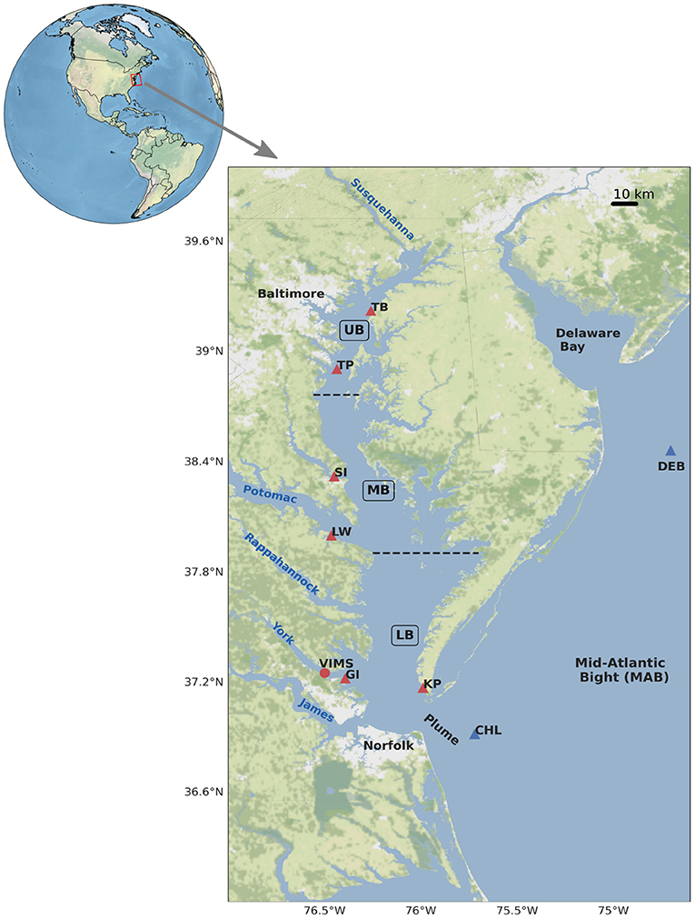
Figure 1. Chesapeake Bay, located on the East Coast of the United States. The blue triangles indicate the Mid-Atlantic Bight (MAB) stations (DEB and CHL) and the red triangles show the Chesapeake Bay stations (TB, TP, SI, LW, GI, and KP). The red circle indicates the VIMS Ferry Pier station. The dashed black lines separate the Lower Bay (LB), Mid Bay (MB) and Upper Bay (UB) regions.
Additional temperature data from the Virginia Institute of Marine Science (VIMS) Ferry Pier (Anderson, 2021) (37.246°N, 76.500°W) available between 1986 and 2003 were used to extend the time series from GI, which originally encompassed the years between 1998 and 2020. A comparison of the overlapping years between the stations, 1998–2003, showed a good agreement (r = 0.99), and a linear regression (GI1986:1997 = a × VIMS1986:1997 + b, where a = 1.03 and b = –0.77) was performed to adjust the amplitude and offset of VIMS Pier Ferry data prior to updating the beginning of the GI time series from 1998 to 1986. Unless noted otherwise, from now on we will refer to GI as the Goodwin Islands time series complemented with the VIMS Pier Ferry data, extending from 1986 to 2020, totalling 35 years of temperature data.
Detailed information about the stations and data used in this study are presented in Table 1. Temperature sensors from all stations were located in the near-surface, between 0.5 and 2 m below sea level, and data were provided at hourly intervals, except at VIMS Ferry Pier and Goodwin Islands, where data were provided every 6 and 15 min, respectively. Record length of the time series varied across stations: from 1986 to 2020 (35 years) at TP, GI, DEB and CHL; from 1994 to 2020 (27 years) at SI and LW; and from 1995 to 2020 (26 years) at TB and KP. Despite the existence of other buoys and stations available in the CB, we restricted our analysis to stations with a minimum record length of 25 years. While Hobday et al. (2016) recommends a minimum record length of 30 years to estimate the baseline climatology for calculating MHWs, Schlegel et al. (2019) demonstrated that reliable results can be obtained with shorter time series.
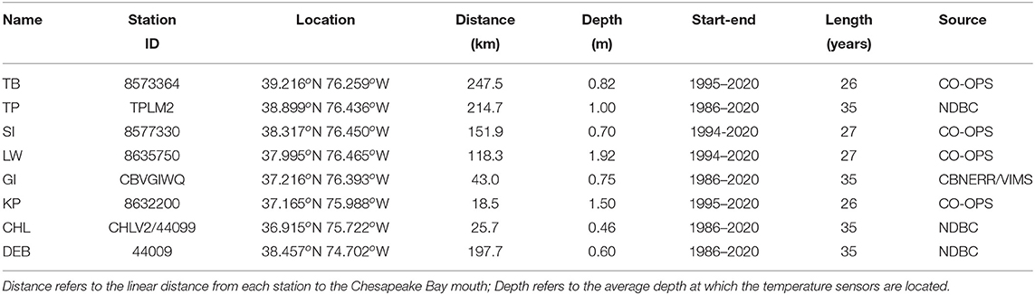
Table 1. Summary of the stations used in this study: TB, Tolchester Beach; TP, Thomas Point; SI, Solomons Island; LW, Lewisetta; GI, Goodwin Island (extended with data from VIMS Ferry Pier between 1986 and 1997, see section 2 Methods); KP, Kiptopeke; CHL, Chesapeake Light Tower; DEB, Delaware Bay buoy.
A zoomed map of the eight stations located within the CB is depicted in Figure 2, with high-resolution, detailed information about the bathymetry. While the stations cover the UB, MB and LB regions, it is important to note that not all stations are situated in the main stem of the bay, for example, SI is located near the mouth of the Patuxent River (Figure 2C), LW near the mouth of the Potomac River (Figure 2D), and GI at the mouth of the York River (Figure 2E). However, significant correlations were observed among all the stations (not shown), revealing a large coherence across the bay, and therefore we may consider that SI, LI and GI also reflect the SST from CB's main stem.
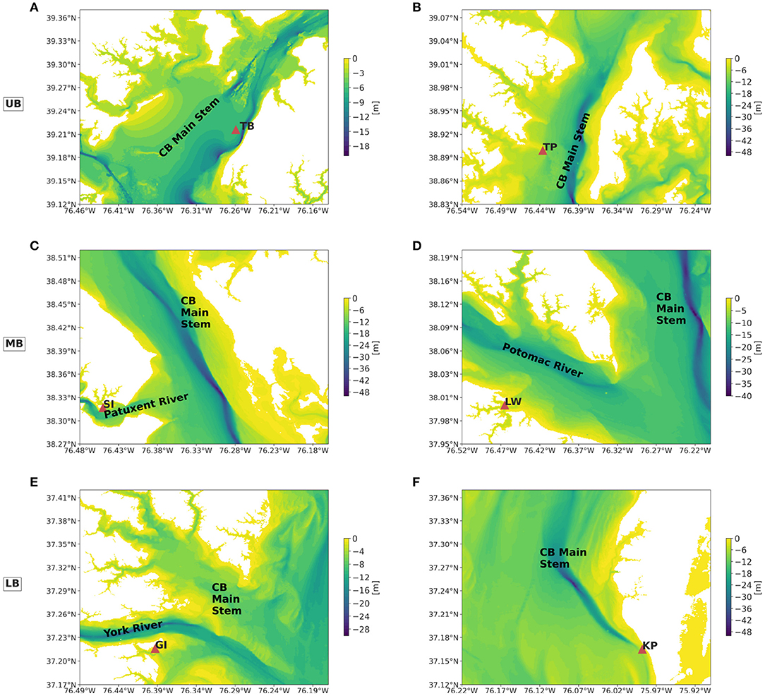
Figure 2. Bathymetry in the vicinity of chesapeake bay stations. (A) Upper Bay: Tolchester Beach (TB) (B) Mid Bay: Thomas Point (TP), (C) Solomons Island (SI), (D) Lower Bay: Lewisetta (LW), (E) Goodwin Island (GI), and (F) Kiptopeke (KP). Bathymetry data was obtained from NOAA National Geophysical Data Center, U.S. Coastal Relief Model Vol.2 - Southeast Atlantic with 3 arc-seconds spatial resolution.
To remove tidal and diurnal temperature variability, all time series were low-passed with a 33 h cutoff, and subsequently binned to daily values. Gaps in the time series of up to 2 days were linearly interpolated (LI) while longer gaps (after June/2002) were filled with SST data from the Multi-scale Ultra-high Resolution (MUR) Sea Surface Temperature Analyses (v4.1) (JPL-MUR-MeaSUREs-Project, 2015), obtained from the Physical Oceanography Distributed Active Archive Center (PODAAC). MUR is a daily, global, gap free, L4 product with spatial resolution of 0.01 x 0.01 degrees, approximately 1 km, currently available from June-2002 to present. SST time series from MUR were extracted from the pixels closest to each station, and compared to the in situ time series. Good agreement between MUR and in situ data was found at all locations (Table 2), and linear regression (Temp = a × MUR + b) was performed to adjust the amplitude and offset of MUR SST data prior to filling the gaps. Table 2, shows that most of the time series gaps were filled, while the remaining gaps correspond to less than 5% of the record length and were positioned before June-2002, when MUR data was not available.
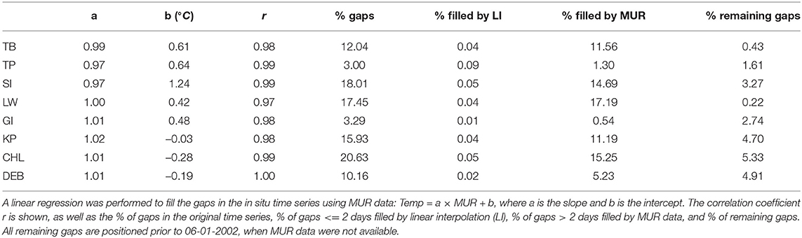
Table 2. Comparison between Multi-scale Ultra-high Resolution (MUR) SST data and in situ temperature time series at each station.
MWHs in this study were determined following the definition proposed by Hobday et al. (2016): a discrete prolonged anomalously warm water event in a particular location. A MHW event occurs when the SST exceeds the 90th percentile (threshold) of its local seasonal climatology for five consecutive days or more [Figure 1 from Hobday et al. (2016)]. The climatology was calculated using an 11-day moving-average window centered on the specific time of the year. Therefore, the definition proposed by Hobday et al. (2016) considers MHWs as relative warm deviations from the baseline climatologies, allowing them to exist at any time of the year, and not only during hot summer months. Note that the climatologies in this study were computed using the longest time series available for each station (Table 1). Climatologies and thresholds for each station are shown in Supplementary Figure 1. The MHW analysis was performed using the Python module “marineHeatWaves” available at https://github.com/ecjoliver/marineHeatWaves, which implements the Hobday et al. (2016) definition.
We explored the following MHW metrics: frequency (number of events per year), duration of the MHW events, MHW days (the sum of number of MHW days per year), average intensity (average temperature anomaly), yearly cumulative intensity (integral of MHW intensities over a year, in °C × days), which is an index that combines both magnitude and duration of heat anomalies and perhaps one of the best indicators for thermal stress on many ecosystems, and MHW days for different categories: Moderate, Strong, Severe and Extreme. The categories were defined based on the level at which temperatures exceed local climatology. According to Hobday et al. (2018), multiples of the 90th percentile difference from the mean climatology define each of the following categories: 1-2x: Moderate; 2-3x: Strong; 3-4x: Severe, and >4x: Extreme. In the present work no Extreme MHW days were detected, and only a single Severe day was found at CHL and DEB, thus when referring to categories, we will only report the Moderate and Strong days. To evaluate long-term trends, least squares linear regression analysis was performed on the yearly averaged MHW characteristics, with slope uncertainties calculated using confidence intervals with 95% confidence level.
A number of studies addressing temperature variability in the CB (Preston, 2004; Najjar et al., 2010; Ding and Elmore, 2015; Hinson et al., 2021) have consistently identified a continuous warming trend throughout the bay. In order to evaluate the role of long-term trends in SST vs. internal variability in affecting trends in MHW characteristics, we calculated the trend attributional ratio (TAR) following Marin et al. (2021):
where TΔSST and TIV represent trends in any MHW characteristics induced from the change in mean SST and from internal variability, respectively. Equation 1 varies between −1, when MHW trends are dominated by internal variability, and 1, when change in mean SST is the major driver affecting MHW trends. A value of 0 denotes that both mechanisms, change in mean SST and internal variability, are equally important drivers.
To compute the TAR, first, a linear trend was removed from the original SST time series, and a new climatology was calculated using these detrended data, which we refer to detrended_clim. Then, using detrended_clim as a new baseline climatology, two sets of MHW trends were calculated: TObs, using as input the original SST time series, and TIV, using the detrended SST time series. Then, TΔSST was constructed simply as TΔSST = TObs − TIV. Finally, those definitions were then used in Equation 1 to estimate TAR.
To investigate the potential co-occurrence of MHWs between different regions within the CB (UB, MB and LB), and between CB and the coastal ocean (CHL and DEB stations), we calculated the Jaccard index (J) (Jaccard, 1901), which can be written as:
where A and B are sets of MHW events observed at two different locations. The Jaccard index measures similarity between a pair of data sets, and lies between J = 0, in the case of absence of co-occurrence, and J = 1, in the case of all events in A also occur in B and vice-versa. In addition, we estimated the timing (lag) of co-occurrence and directionality (e.g., whether A leads or lags B, or if they are synchronous). MHW events were considered to co-occur at two locations when their dates overlapped. We estimated 95% confidence intervals for J using the Bias-Corrected and Accelerated Bootstrap Method with 10,000 iterations, following Efron and Tibshirani (1993).
Prior to the co-occurrence analysis, MHW sets from station pairs at UB (TB and TP), MB (SI and LW), and LB (GI and KP) were combined by calculating their union (e.g., A∪B). This was done in order to increase the spatial representation of different sections of the CB, and consequently it reduced the dimensions of the problem (10 possible combinations of station pairs instead of 28). For events that co-occurred between those combined station pairs, the beginning and ending dates were assigned as the intermediate dates observed at the stations, hence the duration of such events were the average value observed between the stations.
Our objective was to understand the connections of MHWs among the CB-plume-MAB system, and whether there was a preferential directionality for MHW occurrence, with MHWs in the ocean leading to events in the estuary or vice-versa, or alternatively, if extreme heat events in those systems were uncoupled. Understanding the co-occurrence of MHWs and their onset timing between those environments can elucidate possible mechanisms for MHW generation and whether estuaries or coastal ocean can act as potential sources or sinks of extreme events. To the best of our knowledge, this is the first work that explores the connection between MHWs occurring at coastal and estuarine systems.
A global assessment of MHWs and their drivers by Holbrook et al. (2019), have demonstrated that climate modes of variability and ocean/atmosphere teleconnection processes can influence the occurrence of MHWs. In this paper we investigate how different climate indices modulate the likelihood of MHW occurrence in our study region. We focus on three indices known for influencing the CB (e.g., Cronin et al., 2003; Preston, 2004; Lee and Lwiza, 2008; Scully, 2010a; Lee et al., 2013): the NAO, Niño 1+2 and BHI.
NAO data were obtained from the Hurrell principal component (PC)-based NAO index from the National Center for Atmospheric Research, and Niño 1+2 (OISST.v2, 1991–2020 base period) data were obtained from NOAA Climate Prediction Center. BHI was computed following Stahle and Cleaveland (1992), as the normalized sea level pressure difference between Bermuda (32.5°N, 65°W) and New Orleans (30°N, 90°W), using data from NCEP-NCAR Reanalysis. All indices were obtained/computed at monthly intervals, and subsequently linearly interpolated to daily values. Following Holbrook et al. (2019), we calculated the number of days in which MHWs increased or decreased during positive and negative phases of the climate indices.
Confidence levels were calculated using a Monte Carlo approach. This was done by creating synthetic time series with the same periodogram as the climate indices, but generating random, uniformly distributed and independent Fourier coefficient phases (e.g., Rudnick and Davis, 2003). Then, the number of days during positive and negative phases of the synthetic indices were estimated. This calculation was performed 10,000 times for each station and climate index to produce a frequency distribution of the expected number of days. Finally, percentiles of the frequency distribution were used to calculate confidence intervals, and we only report data that is statistically significant at the 95% confidence level.
The number of observed MHW events varied depending on the location and record length (Table 3): in the CB between 46 and 79 events were detected, while 78 and 64 events were found in the plume region and MAB, respectively. Figure 3 shows the percentage of MHWs as a function of seasons: Summer (Jul-Aug-Sep) was the season in which the largest percentage of MHWs were detected, 28–37% (except at GI), almost twice as those during the Winter (Jan-Feb-Mar), which presented the smallest occurrence, 11–22%, except at UB, in which the Fall (Oct-Nov-Dec) presented the smallest number of events, 20%. Spring (Apr-May-Jun) and Fall presented a similar number of MHW events, of nearly a quarter. A recent study by Schlegel et al. (2021) analyzing MHWs over the entire Northwest Atlantic continental shelf, region extending from the MAB to the Labrador Shelf, also shows a similar enhancement of MHWs in the Summer, suggesting that this is not a local effect, but a broader spatial scale pattern. We also analyzed the seasonal variability in MHW characteristics (not shown), but in general, we did not find statistically significant differences among the seasons and stations.
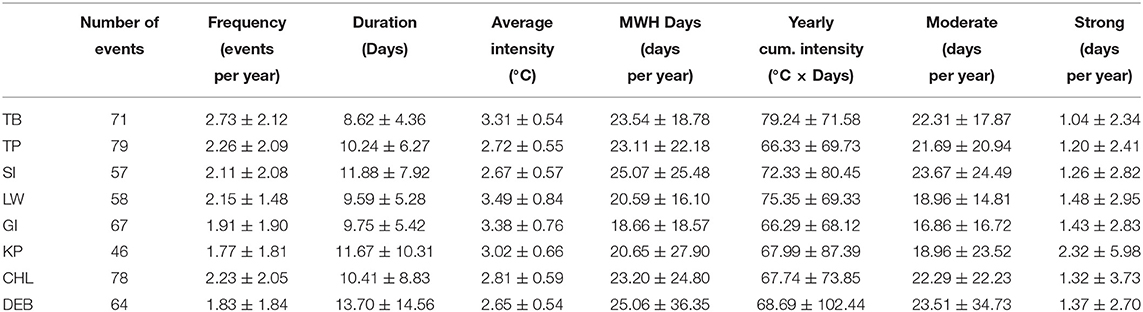
Table 3. Summary of MHW characteristics for each station.
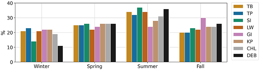
Figure 3. Histogram showing percentage of MHWs events as a function of seasons for each station: Tolchester Beach (TB), Thomas Point (TP), Solomons Island (SI), Lewisetta (LW), Goodwin Island (GI), Kiptopeke (KP), Chesapeake Light Tower (CHL) and Delaware Bay buoy (DEB). Winter was defined as January, February and March; Spring as April, May and June; Summer as July, August and September; Fall as October, November and December.
MHW characteristics in the CB and MAB (plume and ocean) averaged over the entire study period are summarized in Table 3. All MHW metrics investigated here, such as frequency, duration, average intensity, MHW days, yearly cumulative intensity, and MHW categories (Moderate and Strong) were statistically indistinguishable both among stations within the CB, and between CB and MAB stations. On average, 2.1 (± 1.9) MHW events occurred each year in the CB, with maximum values varying between 6 and 8 events per year (Figures 4A,C,E,G). Similar values were also found in the plume and MAB region, with an average of two events per year (± 1.9). Duration of MHWs events in the CB were typically 10.3 (± 6.9) days, but reached up to 39 days in the UB and MB, 50 days in the LB and plume, and over 100 days in the ocean (not shown). Average intensities of MHWs in the CB were 3.1 (± 0.6) °C, with maximum peaks varying between 6 and 8°C (not shown). Total MHW days per year in the bay were on average 21.9 (± 21.9) days, but reached over 120 MHW days, while in the ocean up to 160 MHW days were observed (Figures 5A,C,E,G). The vast majority of MHW days in CB were classified as Moderate, an average of 20.4 (± 20.0) days, contrasting to 1.4 (± 3.4) MHW days which were classified as Strong. Yearly cumulative intensity in the bay was on average 71.2 (± 74.8) °C × days, but reached over 300 °C × days, while over 400 °C × days were observed in the ocean (Figures 5B,D,F,H).
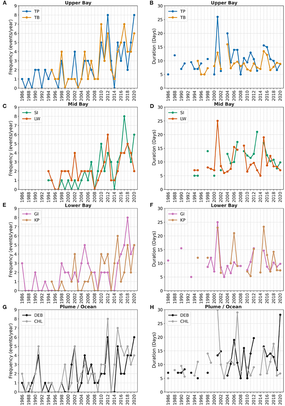
Figure 4. Annual values of (A,C,E,G) MHW Frequency and (B,D,F,H) Duration. (A,B) Upper Bay: Tolchester Beach (TB) and Thomas Point (TP); (C,D) Mid Bay: Solomons Island (SI) and Lewisetta (LW); (E,F) Lower Bay: Goodwin Island (GI) and Kiptopeke (KP); (G,H) Plume/Ocean: Chesapeake Light Tower (CHL) and Delaware Bay buoy (DEB).
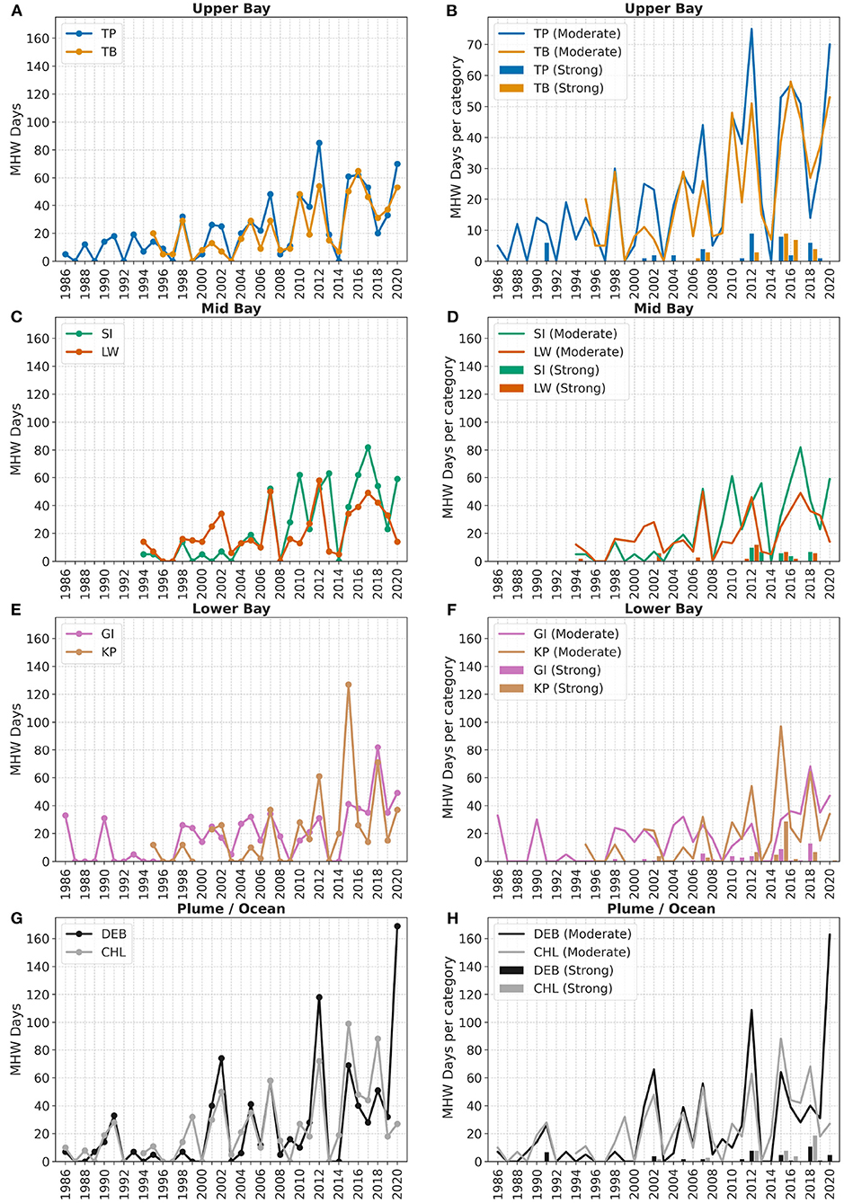
Figure 5. Annual values of (A,C,E,G) MHW Days and (B,D,F,H) MHW Days per category (Moderate and Strong). (A,B) Upper Bay: Tolchester Beach (TB) and Thomas Point (TP); (C,D) Mid Bay: Solomons Island (SI) and Lewisetta (LW); (E,F) Lower Bay: Goodwin Island (GI) and Kiptopeke (KP); (G,H) Plume/Ocean: Chesapeake Light Tower (CHL) and Delaware Bay buoy (DEB).
Interannual variability in MHW characteristics are presented in Figures 4–6, and their respective trends are summarized in Table 4. MHW frequency (Figures 4A,C,E,G) presented large year to year variability, and a temporal increase was observed across the entire study area. Maximum frequency at all stations happened in the last decade (2010–2020), reaching 6–8 events per year, compared to only 4–5 events per year seen prior to 2010. 2012 was the year in which most stations presented maximum frequency, except at TB, SI, GI, KP, however those stations still presented values well above average in that year. It is noteworthy to mention that years without MHW events were not uncommon prior to 2010, but in the last decade only in 2014 a consistent reduction or total absence of MHW events were seen coherently in the whole study area. A significant trend in frequency was observed at all stations, on average 1.4 (± 0.7) annual events per decade in the CB, and a smaller trend in the MAB (plume and ocean) of 1 (± 0.6) annual event per decade.
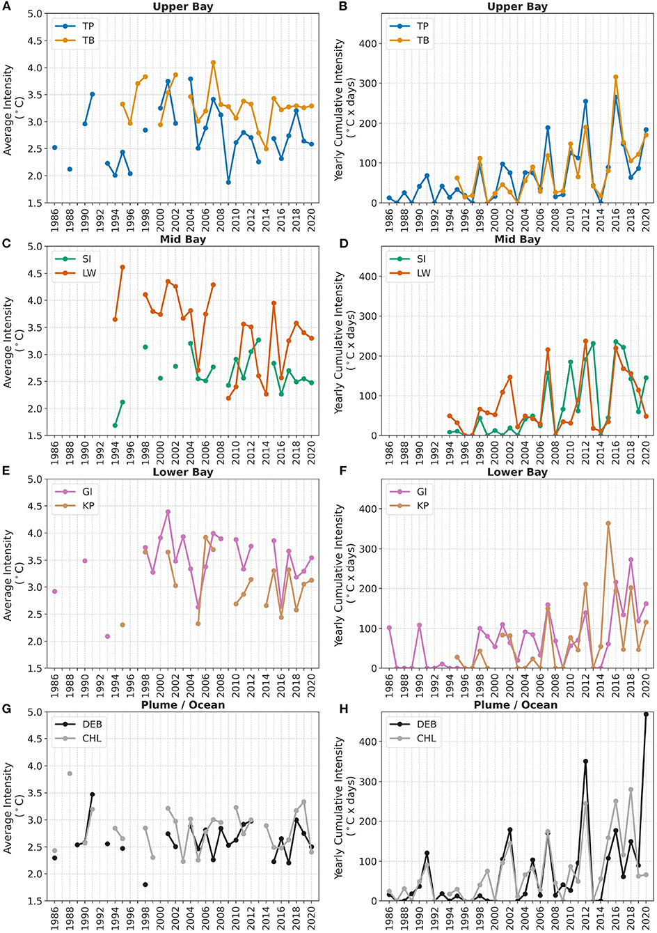
Figure 6. Annual values of (A,C,E,G) MHW Average Intensity and (B,D,F,H) Yearly Cumulative Intensity. (A, B) Upper Bay: Tolchester Beach (TB) and Thomas Point (TP); (C,D) Mid Bay: Solomons Island (SI) and Lewisetta (LW); (E,F) Lower Bay: Goodwin Island (GI) and Kiptopeke (KP); (G,H) Plume/Ocean: Chesapeake Light Tower (CHL) and Delaware Bay buoy (DEB).
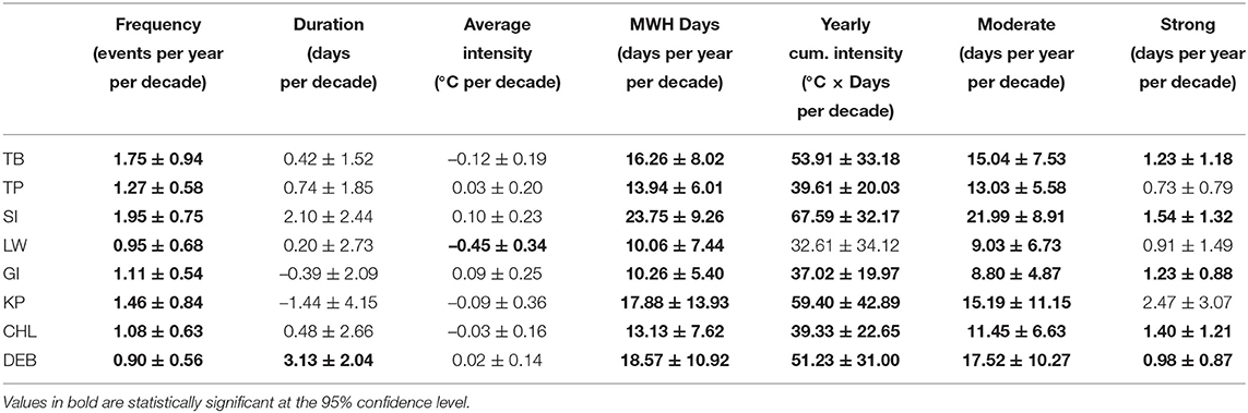
Table 4. Trends of MHW characteristics per decade for each station.
Yearly average duration of events (Figures 4B,D,F,H) did not present a significant trend neither in the CB nor plume, but did present a significant trend at DEB, of 3.1 (± 2.0) days per decade. Coherent patterns in duration can be identified among stations, for example, most locations presented a peak in 2001, 2004, and 2015. MHW days (Figures 5A,C,E,G) refer to the total number of MHW days per year and, therefore, is a metric influenced by both duration and frequency. A significant trend in MHW days was observed across the CB, with an increase of 16.4 (± 8.8) MHW days per decade, and 15.8 (± 9.4) MHW days per decade in the MAB region, as a reflection of the positive trends in frequency. With regard to the MHW categories (Figures 5B,D,F,H), a significant trend was observed for moderate days at all stations, while, for strong days, the trend was significant for the MAB, but in only half of the stations within the CB (TP, SI and GI).
Average MHW intensity (Figures 6A,C,E,G) rarely exceeded 4.5°C in the bay, and small differences, of 0.2–0.8°C, were observed between the station pairs. No trends were significant, except at LW, of –0.45 (± 0.3)°C per decade. Yearly cumulative intensity (Figures 6B,D,F,H), which is an integral of MHW intensities over a year and therefore combines both magnitude and duration of heat anomalies expressing the overall heat stress impacting the ecosystem, showed positive significant trend (except at LW) with average value of 51.5 (± 30.9) °C × days per decade in the CB, and 45.28 (± 27.1) °C × days per decade in the MAB region. This is a reflection of the significant increase in frequency of MHW events in the study area, previously discussed. Peaks generally coincide between pairs of stations but not always across all regions. A few peaks however were common to all locations, for instance 2007, 2012 and 2016.
The large value in 2012 for instance, is a consequence of a single extreme event, named the Northwest Atlantic 2012 (NWA 2012), which gained significant attention by the scientific community (Mills et al., 2013; Chen et al., 2014, 2015; Frölicher and Laufkötter, 2018; Hobday et al., 2018, among others). The NWA 2012 was considered the largest most intense extreme event that happened in the preceding 30 years in the NW Atlantic (Mills et al., 2013). Despite the importance of that singular event, our results showed an increase of extreme events with similar or higher cumulative intensity (not shown) throughout the whole study area in more recent years, which is reflected by the large peaks of yearly cumulative intensity (Figures 6B,D,F,H).
TAR was calculated according to Equation 1 following Marin et al. (2021), and results are presented in Table 5 for the MHW characteristics with statistically significant trends. Positive TAR means that long-term changes in SST is the main driver of MHW trends, negative TAR points to internal variability as the dominant driver, and TAR equal to zero indicates that both mechanisms are equally important in driving the observed MHW trends.
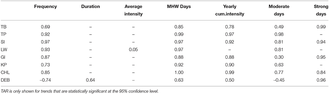
Table 5. Trend attributional ratio (TAR) for MHW characteristics trends for each station.
In the CB and plume region (CHL), TAR values were positive for all trends (statistically significant): frequency varied between 0.69 and 0.97; MHW days between 0.85 and 1.00; yearly cumulative intensity between 0.78 and 0.99 (except at LW, where trend was not significant); moderate days between 0.30 and 0.98, and strong days between 0.84 and 0.99 (at TB, SI and GI, where trend was significant). Intensity was only significant at LW, where TAR was close to zero (0.05). At DEB, TAR values were positive for most MHW characteristics, between 0.50 and 0.96, however negative values were observed for frequency and moderate days, –0.74 and –0.45, respectively. In summary, long-term warming of SST was the dominant driver of MHW trends in our study area, except for MHW frequency and moderate days at DEB.
The Jaccard Index, calculated according to Equation 2, provides a measure of co-occurrence of MHWs between pairs of locations (A and B) in our study area, and it is presented in Table 6. The Jaccard index varies between J = 1, in the case of all events in A and B co-occur, and J = 0, in the case there is no overlap of any events between A and B. For the events that were found to co-occur between two locations, we calculated the percentage that are synchronous, meaning that MHWs started at the same time at A and B, and calculated the percentage of MHWs that began at A (A leads B) or at B (A lags B), as well their respective lags in days.
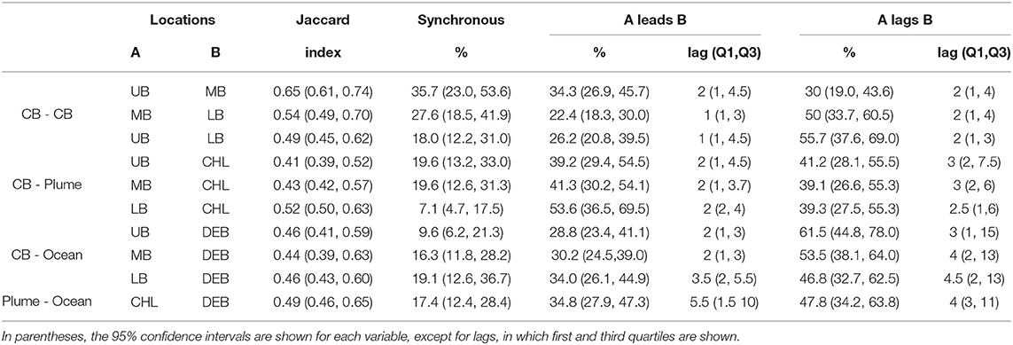
Table 6. Summary of co-occurrence analysis for each station, showing the: Jaccard Index, % of synchronous events, % of events which location A leads B, % of events which location A lags B, and their respective lags in days.
Within the CB, co-occurrence (Jaccard Index) varied between 0.49 and 0.65, with largest values between adjacent locations (UB and MB, MB and LB) and smallest between UB and LB. Synchronous events happened 18–36% of the time, and no clear directionality was observed between UB and MB, however, LB led both MB and UB for over half of the time, with lags of 2 days in both cases.
Co-occurrence between plume (CHL) and MB and UB varied between 0.41 and 0.43, with nearly 20% of events being synchronous, and only 2% difference between plume leading vs. lagging, hence no clear preferred directionality was observed. As expected due to their proximity, co-occurrence between LB and plume presented a larger value, of 0.52. Only 7% of events were synchronous, and a slight preference was found for the LB leading plume, over 54 vs. 40% of plume leading LB, with lags of 2 and 2.5 days, respectively.
CB and ocean (DEB) co-occurrence was nearly uniform across different regions of the CB, varying only between 0.44 and 0.46. Ocean led MHWs in the CB during 47–61% of the time, with lags of 3–4.5 days. CB on the other hand, led MHWs in the ocean during 29–34% of the time, with lags of 2–3.5 days. Synchronous events were not negligible, they occurred 10–19% of the time. A similar pattern was observed between plume and ocean, with co-occurrence of 0.59, 17% of synchronous events, 48% of ocean leading plume at a 4 days lag, vs. 35% of plume leading ocean at 5.5 days lag.
The percentage change in MHW occurrences at different phases of the climate indices addressed here are shown in Figure 7. The black lines show the percentage of MHW days observed over the full study period, regardless of the phases of the climate indices. Note that the black lines deviate from the 10% expected value due to the 5-day threshold requirement from the definition of MHWs used here.
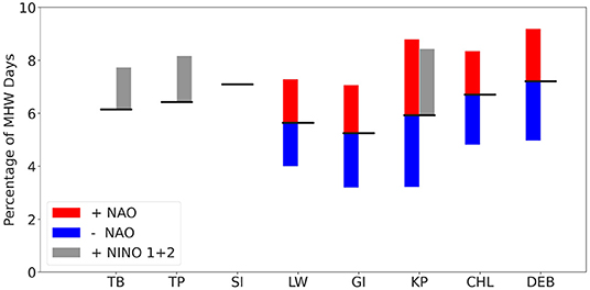
Figure 7. The percentage change in MHW occurrences at different phases of the North Atlantic Oscillation (NAO) and the Niño 1+2 indices at each station: Tolchester Beach (TB), Thomas Point (TP), Solomons Island (SI), Lewisetta (LW), Goodwin Island (GI), Kiptopeke (KP), Chesapeake Light Tower (CHL) and Delaware Bay buoy (DEB). Red and gray bars denote positive phases of NAO and Niño 1+2, respectively, while blue bars denote negative phase of NAO. The black lines indicate the percentage of MHW days observed over the full study period. Values above the black lines indicate enhancement of MHW days, while values below the black line indicates decrease of MHW days.
From the three indices explored, only Niño 1+2 and NAO presented a significant relationship with the MHW occurrences, while no association was observed with the BHI at any of the stations analyzed. For the NAO, we observed that the relationship was maximized at 1 month lag, coinciding with the lag that maximized correlations between SST anomalies and NAO (not shown), thus we report results comparing MHWs with the NAO values of the preceding month. Such a relationship was not observed for Niño 1+2, nor for BHI, in which their maximized correlations with SST anomalies (not shown) occurred at zero lag.
Niño 1+2 had a significant relationship only at three stations: TB and TP in the UB, and KP at LB. During the positive phase, a 2–3% enhancement of MHW days was observed at those stations, while no relationship was observed at the negative phase. NAO had a significant relationship with a larger number of stations: LW at MB, GI and KP at LB, and CHL and DEB at the MAB. A 2–3% enhancement of MHW days was observed during the positive phase of NAO, while a suppression, with similar magnitude, was observed during the negative phase.
Long-term warming trends in response to climate change have been detected in a number of estuaries around the globe (e.g., Ashizawa and Cole, 1994; Seekell and Pace, 2011; Oczkowski et al., 2015; Jackson et al., 2021), and the CB is no exception (Preston, 2004; Najjar et al., 2010; Ding and Elmore, 2015; Hinson et al., 2021). However, our current knowledge about extreme events, such as MHWs, is still lacking in those environments. A limited number of studies have targeted a few unique MHW events, focusing on their impact on the estuarine ecosystem (e.g., Shields et al., 2019; Aoki et al., 2021; Johnson et al., 2021), while a systematic physical assessment of MHWs has not been previously pursued. The present work addresses this gap by characterizing MHWs in an estuary (CB), evaluating trends in MHW characteristics, their relationship to climate modes of variability and connection to the MHWs occurring in the adjacent coastal ocean.
Our assessment demonstrates that average MHW metrics were similar among the different regions of the CB: UB, MB and LB, and that they did not significantly differ from those metrics observed in the plume nor in the adjacent coastal ocean. Furthermore, significant trends were observed consistently throughout our study area for MHW frequency, and consequently, for MHW days and yearly cumulative intensity. While global estimates have found increasing trends in average MHW intensity and duration (Oliver et al., 2018), we detected a significant increase in duration only in the ocean (DEB), but no significant increase in intensity was observed in the bay, plume or ocean. Relative to the climatology baseline adopted here (1986–2020), the trends found in our work suggest that within the next 50 years MHWs will be observed with monthly frequency in the CB, while by the end of the century it is expected that MHWs will be present over half of the year.
According to the TAR analysis conducted here, the observed MHW trends discussed above were primarily driven by long-term warming across the CB. In fact, a recent assessment by Marin et al. (2021), showed that this is also the case for the vast majority of coastal regions worldwide. The mechanisms leading to CB warming in recent decades have been recently investigated by Hinson et al. (2021). Through numerical modeling sensitivity experiments, the authors evaluated the relative contribution of rivers, atmosphere, and ocean to the changes in bay temperatures between 1985 and 2019, a similar period addressed in our study. According to the authors, the influence of riverine warming impacted a relatively small region, restricted to the heads of the tributaries, while the influence of oceanic waters in the CB surface warming was only seen in the southern portion of the LB near the CB mouth. The role of atmospheric forcing, including both increasing air temperatures and downwelling longwave radiation, was the dominant mechanism, leading to a fairly spatially homogeneous surface warming trend throughout the CB main stem. This spatially coherent warming driven by large-scale atmospheric forcing may explain the large agreement in the MHW trends and TAR observed among the different regions of the CB found in our study.
The distribution of temperature anomalies in the CB (using all 6 stations) is shown in Figure 8, comparing observations from the last decade (2010–2020) to the preceding years from our time series. A clear shift in the mean temperature anomalies can be observed through time, showing a progressive warming of CB SST anomalies, and illustrates the increase in the probability of events crossing the MHW threshold. Our TAR analysis also demonstrated that both plume (CHL) and ocean (DEB) trends were mainly driven by long-term changes in SST, with the exception of MHW frequency and moderate days at DEB, in which internal variability was main driver, and deserves further investigation, but remains beyond the scope of this work, that focuses on the CB.
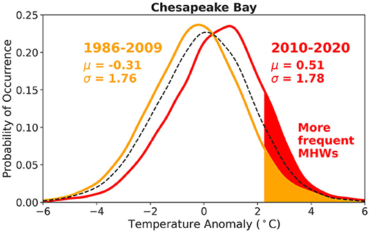
Figure 8. Probability of occurrence of sea surface temperature anomalies in the Chesapeake Bay. The stations used in this analysis were: Tolchester Beach (TB), Thomas Point (TP), Solomons Island (SI), Lewisetta (LW), Goodwin Island (GI), and Kiptopeke (KP). Yellow corresponds to years between 1986 and 2009, red corresponds to the most recent decade, 2010–2020, and black dashed line refers to all years combined, 1986–2020. Shaded regions show the area above the 90th percentile threshold, estimated from the entire time series. Mean (μ) and standard deviation (σ) values in °C are indicated. The enhanced red shaded area indicates an increase in likelihood of MHWs in the last decade.
Our study demonstrated that within the CB, approximately 50–65% of MHW events co-occurred between different regions of the bay (UB, MB, LB), and with relatively short lags, of generally 2 days or less. This reveals that the majority of MHWs are not locally restricted, but instead, they tend to occur coherently across the entire length of the bay, which spans over 320 km. Elevated co-occurrence of MHWs, of 40–50%, was also observed between CB-plume-ocean systems, demonstrating a strong connection among those different environments, with lags of 2–5.5 days, but we did not identify preferential sources or sinks of MHWs. This large co-occurrence observed throughout the entire length of our study area, and the relative short lags, suggests that coherent large-scale forcing is driving MHWs in this region.
A dynamical understanding of surface MHWs can be obtained through the analysis of a surface mixed layer temperature budget (e.g., Moisan and Niiler, 1998; Oliver, 2021; Schlegel et al., 2021), which can be written as:
where Tmix is the average temperature in the surface mixed layer, Qnet is the net air sea heat fluxes, ρ is the average seawater density, cp is the specific heat of seawater, H is the surface mixed layer depth, umix refers to horizontal velocities in the mixed layer, and R is a residual term. The left hand side of Equation 3 refers to the time rate of change of temperature within the surface mixed layer, and on the right hand side the first term refers to the air-sea heat flux into the mixed layer, the second term refers to convergence of heat in the mixed layer due to horizontal advection, and the third term (residual) includes vertical advection, entrainment, mixing, as well as penetrating radiation that passes below the mixed layer.
While resolving all the terms in the mixed layer heat budget remains beyond the scope of this work, examination of Equation 3 can aid the interpretation of our results and allows the inspection of possible mechanisms driving in SST variations associated with MHWs in our study area. The first two terms on the right hand side of Equation 3, air-sea heat flux and horizontal advection, have been shown to be the leading drivers of temperature changes associated with MHWs around the globe (Oliver, 2021), while R often accounts for a smaller proportion of mixed-layer temperature changes.
Although it is plausible that advection could explain a fraction of co-occurrence between adjacent locations (e.g., plume and LB, UB and MB, MB, and LB), it is unlikely that advection played a significant role between stations situated farther apart due to the short observed lags. For example, UB and DEB which are situated over 400 km apart (Table 1), presented co-occurrence with a median lag of 3 days (Table 6), and in order for advection to explain the observed co-occurrence, an advective velocity umix over 1.5 m/s would be required, which is unrealistic. As a matter of fact, estimates of CB residence time are two orders of magnitude larger than the observed lags. For example, Du and Shen (2016) showed that average residence time of surface waters in the CB reach over 6 months in the MB, and over 9 months in the UB. Therefore, the most likely candidate to drive the largely coherent MHWs in the CB and plume-ocean region is air-sea heat flux. In fact, a recent study analyzing MHW drivers by Schlegel et al. (2021), found that over the Northwest Atlantic continental shelf half of MHWs are triggered by positive heat flux into the ocean, hence evidencing the important role that large-scale atmospheric forcing plays over our study area.
Furthermore, our work illustrates a complex spatial relationship between MHWs and climate indices (Figure 7). In fact, the relationship between large-scale climate modes of variability and local ocean and weather conditions is often not straightforward (Stenseth et al., 2003), particularly in the CB which is strongly influenced by the surrounding watershed (Kimmel et al., 2009). Nevertheless, we found a statistical link between Niño 1+2 and NAO with the modulation of MHWs across different regions of the CB, but no relationship was detected with the BHI. The enhancement of MHW days in the UB was associated with the positive phase of Niño 1+2, while enhancement and suppression of MHW days both in the MB and LB were associated with positive and negative phases of NAO, respectively. These modulations associated with Niño 1+2 and NAO are not insignificant as they correspond to a change in the likelihood of MHW occurrence of 30–50%. While the modulation of MHW occurrence is generally consistent with changes in SST anomalies (not shown), as pointed out by Holbrook et al. (2019), significant statistical relationships do not necessarily indicate causal links. Yet, understanding the connection between climate indices and MHW occurrence, can be important for the predictability of those events. Future efforts should focus on addressing the dynamical mechanisms behind these connections in order to further improve predictive models of these extreme events, which have profound effects on the bay's ecosystem.
Estuaries are valuable environments, amongst the most productive ecosystems on our planet, but have been severely threatened by climate change. As temperatures continue to rise throughout the twenty-first century, it is expected that estuarine systems will experience significant habitat loss and water quality degradation resulting from eutrophication, deoxygenation, increase in harmful algal bloom events, etc. A major recurring problem that CB faces is eutrophication-induced hypoxia, consistently observed annually in bottom waters during the summer, resulting in the formation of a large dead zone; as the CB continues to warm, the total annual hypoxic volume is expected to increase (Irby et al., 2018; Ni et al., 2019). Moreover, the future increase in MHW events as suggested in our study, could aggravate hypoxia in the bay by strengthening water column stratification, enhancing eutrophication, exacerbating the oxygen consumption/uptake and decreasing oxygen solubility, therefore potentially pushing the CB ecosystem past a dangerous tipping point.
While the impact of short-lived extreme events, such as MHWs, has not been fully evaluated to the overall water quality in the CB, they have been linked to the mortality of SAV (Moore and Jarvis, 2008; Shields et al., 2019; Johnson et al., 2021), an important ecosystem that provides nursery habitat, improves water quality and sequesters carbon (Lefcheck et al., 2017). We can expect such die-offs to become more frequent in the future with the MHWs projected to increase. Future continuous monitoring efforts in the CB should not only focus on the surface, but also include high-frequency water column surveys (e.g., Mazzini et al., 2019) of physical and biogeochemical parameters in order to fully evaluate the three-dimensional impacts of MHWs on the CB health.
Warming trends of estuarine environments in response to climate change have been investigated in a number of estuaries across the globe, however to our best knowledge, no research has been conducted addressing short term, extreme temperature events, or MHWs, in these environments. This work provides a pioneer contribution in characterizing MHWs in an estuarine system, analyzing their trends, their relationship to climate modes of variability, and connection to the coastal ocean. This novel research was made possible thanks to an unprecedented long-term in situ SST record available, over 30 years long, in the largest and most productive estuary in the US: the Chesapeake Bay.
Significant positive trends were detected for MHW frequency, MHW days and yearly cumulative intensity (an indicator of heat stress for marine systems), and they were attributed to long-term warming observed in the Bay. If these trends persist, by the end of the century the Chesapeake Bay will reach a semi-permanent MHW state, when extreme temperatures will be present over half of the year. The impact of MHWs will have profound consequences to the estuarine ecosystem, and future management decisions should not only focus on the effect of long-term temperature changes, but also take into consideration these short, acute events, which could have severe impacts well beyond their lifetime.
Our analysis demonstrated that the majority of MHW events occurred coherently throughout the Upper, Mid and Lower Bay and between Chesapeake Bay and the Mid Atlantic Bight, suggesting that atmospheric heat flux is the dominant driver of MHWs in this region. Yet, a heat budget analysis should be pursued to properly quantify the relative contribution of each of the mechanisms responsible for SST changes driving MHWs in the Bay (Equation 3). In addition, a characterization of environmental settings (winds, river discharge, etc) preceding the onset of MHW events, must be investigated to understand the conditions prone to MHWs triggering.
While this work is the first step in assessing MHWs in an estuarine environment, it is important to emphasize that our analysis was restricted to the surface waters only. Future research should target MHWs in subsurface estuarine waters since they can have important implications for benthic communities as well as bottom hypoxia and anoxia. Finally, future studies should pursue a systematic comparison of MHWs in different estuary types, morphologies, sizes, flushing times, and contrasting coastal ocean regions (e.g., eastern vs. western boundary systems), in order to further advance our dynamical understanding of MHWs in estuarine systems and consequently improve the predictability of those important and impactful extreme events.
All datasets used in this study are publicly available. In situ temperature records can be found at: CBNERR-VA (https://cdmo.baruch.sc.edu/dges/), NDBC (https://www.ndbc.noaa.gov/), CO-OPS (https://tidesandcurrents.noaa.gov/), VIMS Ferry Pier (https://scholarworks.wm.edu/data/436/). Sea surface temperature data from version 4 Multiscale Ultrahigh Resolution (MUR) L4, can be found at: https://podaac.jpl.nasa.gov/dataset/MUR-JPL-L4-GLOB-v4.1. Climate indices can be found at: NINO 1+2 (https://www.cpc.ncep.noaa.gov/products/monitoring_and_data/oadata.shtml) and North Atlantic Oscillation (https://climatedataguide.ucar.edu/climate-data/hurrell-north-atlantic-oscillation-nao-index-pc-based). Sea level pressure data from NCEP/NCAR Reanalysis used to calculate the Bermuda High Index (BHI) can be found at: https://www.psl.noaa.gov/data/gridded/data.ncep.reanalysis.derived.html.
PM lead the writing and analysis of co-occurrence and climate indices. CP processed and analyzed the in situ and satellite temperature datasets, lead the MHW analysis, prepared all figures, and contributed to the writing. Both authors contributed equally to the intellectual development of the manuscript.
The authors declare that the research was conducted in the absence of any commercial or financial relationships that could be construed as a potential conflict of interest.
All claims expressed in this article are solely those of the authors and do not necessarily represent those of their affiliated organizations, or those of the publisher, the editors and the reviewers. Any product that may be evaluated in this article, or claim that may be made by its manufacturer, is not guaranteed or endorsed by the publisher.
We would like to thank the National Data Buoy Center (NDBC), the Center for Operational Oceanographic Products and Services (CO-OPS), the Chesapeake Bay National Estuarine Research Reserve in Virginia (CBNERR-VA), Physical Oceanography Distributed Active Archive Center (PO.DAAC), National Center for Atmospheric Research (NCAR) and NOAA Climate Prediction Center (CPC) for providing data used in this study. We would like to thank Gary F. Anderson from the Virginia Institute of Marine Science for the VIMS Pier Ferry dataset. We would also like to thank Dr. Eric C. J. Oliver for making the Python module marineHeatWaves publicly available. We also thank the two reviewers for their helpful and insightful comments. This paper is Contribution No. 4066 of the Virginia Institute of Marine Science, William and Mary.
The Supplementary Material for this article can be found online at: https://www.frontiersin.org/articles/10.3389/fmars.2021.750265/full#supplementary-material
Anderson, G. F.. (2021). Vims Ferry Pier Ambient Water Monitoring, Salinity and Temperature, Daily Summary 1947-2003. William & Mary.
Aoki, L. R., McGlathery, K. J., Wiberg, P. L., Oreska, M. P., Berger, A. C., Berg, P., et al. (2021). Seagrass recovery following marine heat wave influences sediment carbon stocks. Front. Mar. Sci. 7:576784. doi: 10.3389/fmars.2020.576784
Ashizawa, D., and Cole, J. J. (1994). Long-term temperature trends of the hudson river: a study of the historical data. Estuaries 17, 166–171. doi: 10.2307/1352565
Boicourt, W. C.. (1973). The Circulation of Water on the Continental Shelf from Chesapeake Bay to Cape Hatteras (Ph.D. dissertation). Johns Hopkins University.
Brian Dzwonkowski, B., and Yan, X.-H. (2005). Tracking of a chesapeake bay estuarine outflow plume with satellite-based ocean color data. Cont. Shelf Res. 25, 1942–1958. doi: 10.1016/j.csr.2005.06.011
Caputi, N., Kangas, M., Denham, A., Feng, M., Pearce, A., Hetzel, Y., et al. (2016). Management adaptation of invertebrate fisheries to an extreme marine heat wave event at a global warming hot spot. Ecol. Evol. 6, 3583–3593. doi: 10.1002/ece3.2137
Cavole, L., Demko, A., Diner, R., Giddings, A., Koester, I., Pagniello, C., et al. (2016). Biological impacts of the 2013–2015 warm-water anomaly in the northeast pacific: winners, losers, and the future. Oceanography 29, 273–285. doi: 10.5670/oceanog.2016.32
Chen, K., Gawarkiewicz, G., Kwon, Y. O., and Zhang, W. G. (2015). The role of atmospheric forcing versus ocean advection during the extreme warming of the northeast us continental shelf in 2012. J. Geophys. Res. Oceans 120, 4324–4339. doi: 10.1002/2014JC010547
Chen, K., Gawarkiewicz, G. G., Lentz, S. J., and Bane, J. M. (2014). Diagnosing the warming of the northeastern U.S. Coastal Ocean in 2012: a linkage between the atmospheric jet stream variability and ocean response. J. Geophys. Res. Oceans 119, 218–227. doi: 10.1002/2013JC009393
Cloern, J. E., Foster, S. Q., and Kleckner, A. E. (2014). Phytoplankton primary production in the world's estuarine-coastal ecosystems. Biogeosciences 11, 2477–2501. doi: 10.5194/bg-11-2477-2014
Cronin, T. M., Dwyer, G. S., Kamiya, T., Schwede, S., and Willard, D. A. (2003). Medieval warm period, little ice age and 20th century temperature variability from chesapeake bay. Glob. Planet Change 36, 17–29. doi: 10.1016/S0921-8181(02)00161-3
Ding, H., and Elmore, A. J. (2015). Spatio-temporal Patterns in Water Surface Temperature from Landsat Time Series Data in the Chesapeake Bay, U.S.A. Remote Sens. Environ. 168, 335–348 doi: 10.1016/j.rse.2015.07.009
Du, J., and Shen, J. (2016). water residence time in chesapeake bay for 1980–2012. J. Mar. Syst. 164, 101–111. doi: 10.1016/j.jmarsys.2016.08.011
Eakin, C. M., Sweatman, H. P. A., and Brainard, R. E. (2019). The 2014-2017 global-scale coral bleaching event: insights and impacts. Coral Reefs 38, 539–545. doi: 10.1007/s00338-019-01844-2
Efron, B., and Tibshirani, R. (1993). An Introduction to the Bootstrap. New York, NY: Chapman and Hall.
Ehlers, A., Worm, B., and Reusch, T. (2008). Importance of genetic diversity in eelgrass zostera marina for its resilience to global warming. Mar. Ecol. Prog Ser. 355, 1–7. doi: 10.3354/meps07369
Filbee-Dexter, K., Wernberg, T., Grace, S. P., Thormar, J., Fredriksen, S., Narvaez, C. N., et al. (2020). Marine heatwaves and the collapse of marginal north atlantic kelp forests. Sci. Rep. 10:13388. doi: 10.1038/s41598-020-70273-x
Fraser, M. W., Kendrick, G. A., Statton, J., Hovey, R. K., Zavala-Perez, A., and Walker, D. I. (2014). Extreme climate events lower resilience of foundation seagrass at edge of biogeographical range. J. Ecol. 102, 1528–1536. doi: 10.1111/1365-2745.12300
Frölicher, T. L., and Laufkötter, C. (2018). Emerging risks from marine heat waves. Nat. Commun. 9, 2015–2018. doi: 10.1038/s41467-018-03163-6
Garrabou, J., Coma, R., Bensoussan, N., Bally, M., Chevaldonn, P., Cigliano, M., et al. (2009). Mass mortality in northwestern mediterranean rocky benthic communities: effects of the 2003 heat wave. Glob. Chang Biol. 15, 1090–1103. doi: 10.1111/j.1365-2486.2008.01823.x
Gobler, C. J.. (2020). Climate change and harmful algal blooms: insights and perspective. Harmful Algae 91:101731. doi: 10.1016/j.hal.2019.101731
Guo, X., and Valle-Levinson, A. (2007). Tidal effects on estuarine circulation and outflow plume in the chesapeake bay. Cont Shelf Res. 27, 20–42. doi: 10.1016/j.csr.2006.08.009
Hinson, K., Friedrichs, M. A. M., St-Laurent, P., Da, F., and Najjar, R. G. (2021). Extent and causes of chesapeake bay warming. J. Am. Water Resour. Assoc. 1–21. doi: 10.1111/1752-1688.12916
Hobday, A., Oliver, E., Sen Gupta, A., Benthuysen, J., Burrows, M., Donat, M., et al. (2018). Categorizing and naming marine heatwaves. Oceanography 31, 162–173. doi: 10.5670/oceanog.2018.205
Hobday, A. J., Alexander, L. V., Perkins, S. E., Smale, D. A., Straub, S. C., Oliver, E. C., et al. (2016). A hierarchical approach to defining marine heatwaves. Prog Oceanogr. 141, 227–238. doi: 10.1016/j.pocean.2015.12.014
Holbrook, N. J., Scannell, H. A., Sen Gupta, A., Benthuysen, J. A., Feng, M., Oliver, E. C. J., et al. (2019). A global assessment of marine heatwaves and their drivers. Nat. Commun. 10:2624. doi: 10.1038/s41467-019-10206-z
Hughes, T. P., Kerry, J. T., Álvarez-Noriega, M., Álvarez-Romero, J. G., Anderson, K. D., Baird, A. H., et al. (2017). Global warming and recurrent mass bleaching of corals. Nature 543, 373–377. doi: 10.1038/nature21707
Irby, I. D., Friedrichs, M. A. M., Da, F., and Hinson, K. E. (2018). The competing impacts of climate change and nutrient reductions on dissolved oxygen in chesapeake bay. Biogeosciences 15, 2649–2668. doi: 10.5194/bg-15-2649-2018
Jaccard, P.. (1901). Distribution de la flore alpine dans le bassin des dranses et dans quelques rgions voisines. Bull. Soc. Vaudoise des Sci. Nat. 37, 241–272.
Jackson, J. M., Bianucci, L., Hannah, C. G., and Carmack, E. C. (2021). Deep waters in british columbia mainland fjords show rapid warming and deoxygenation from 1951 to 2020. Geophys. Res. Lett. 48, 1–9. doi: 10.1029/2020GL091094
Jacox, M. G.. (2019). Marine heatwaves in a changing climate. Nature 571, 485–487. doi: 10.1038/d41586-019-02196-1
Jiang, L., and Xia, M. (2016). Dynamics of the chesapeake bay outflow plume: realistic plume simulation and its seasonal and interannual variability. J. Geophys. Res. Oceans 121, 1424–1445. doi: 10.1002/2015JC011191
Johnson, A. J., Shields, E. C., Kendrick, G. A., and Orth, R. J. (2021). Recovery dynamics of the seagrass zostera marina following mass mortalities from two extreme climatic events. Estuar. Coasts 44, 535–544. doi: 10.1007/s12237-020-00816-y
JPL-MUR-MeaSUREs-Project (2015). Ghrsst Level 4 Mur Global Foundation Sea Surface Temperature Analysis (v4.1). PO.DAAC, CA.
Kimmel, D., Miller, W., Harding, L., Houde, E., and Roman, M. (2009). Estuarine ecosystem response captured using a synoptic climatology. Estuar. Coasts 32, 403–409. doi: 10.1007/s12237-009-9147-y
Lee, Y., Boynton, W., Li, M., and Li, Y. (2013). Role of late winter spring wind influencing summer hypoxia in chesapeake bay. Estuar. Coasts 36, 683–696. doi: 10.1007/s12237-013-9592-5
Lee, Y., and Lwiza, K. (2008). Factors driving bottom salinity variability in the chesapeake bay. Cont Shelf Res. 28, 1352–1362. doi: 10.1016/j.csr.2008.03.016
Lefcheck, J. S., Wilcox, D. J., Murphy, R. R., Marion, S. R., and Orth, R. J. (2017). Multiple stressors threaten the imperiled coastal foundation species eelgrass (Zostera Marina) in chesapeake bay, USA. Glob. Chang Biol. 23, 3474–3483. doi: 10.1111/gcb.13623
Li, Y., and Li, M. (2011). Effects of winds on stratification and circulation in a partially mixed estuary. J. Geophys. Res. 116:C12012. doi: 10.1029/2010JC006893
Marb, N., and Duarte, C. M. (2010). Mediterranean warming triggers seagrass (posidonia oceanica) shoot mortality. Glob. Chang Biol. 16, 2366–2375. doi: 10.1111/j.1365-2486.2009.02130.x
Marin, M., Feng, M., Phillips, H. E., and Bindoff, N. L. (2021). A global, multiproduct analysis of coastal marine heatwaves: distribution, characteristics, and long term trends. J. Geophys. Res. Oceans 126, 1–17. doi: 10.1029/2020JC016708
Mazzini, P. L., Chant, R. J., Scully, M. E., Wilkin, J., Hunter, E. J., and Nidzieko, N. J. (2019). The impact of wind forcing on the thermal wind shear of a river plume. J. Geophys. Res. Oceans 124, 7908–7925. doi: 10.1029/2019JC015259
McCabe, R. M., Hickey, B. M., Kudela, R. M., Lefebvre, K. A., Adams, N. G., Bill, B. D., et al. (2016). An unprecedented coastwide toxic algal bloom linked to anomalous ocean conditions. Geophys. Res. Lett. 43, 10, 366–10,376. doi: 10.1002/2016GL070023
Mills, K., Pershing, A., Brown, C., Chen, Y., Chiang, F.-S., Holland, D., et al. (2013). Fisheries management in a changing climate: lessons from the 2012 ocean heat wave in the northwest atlantic. Oceanography 26, 191–195. doi: 10.5670/oceanog.2013.27
Moisan, J. R., and Niiler, P. P. (1998). The seasonal heat budget of the north pacific: net heat flux and heat storage rates (1950–1990). J. Phys. Oceanogr. 28, 401–421. doi: 10.1175/1520-0485(1998)028h0401:TSHBOTi2.0.CO;2
Moore, K. A., and Jarvis, J. C. (2008). Environmental factors affecting recent summertime eelgrass diebacks in the lower chesapeake bay: implications for long-term persistence. J. Coastal Res. 10055, 135–147. doi: 10.2112/SI55-014
Najjar, R. G., Pyke, C. R., Adams, M. B., Breitburg, D., Hershner, C., Kemp, M., et al. (2010). Potential climate-change impacts on the chesapeake bay. Estuar Coast Shelf Sci. 86, 1–20. doi: 10.1016/j.ecss.2009.09.026
Ni, W., Li, M., Ross, A. C., and Najjar, R. G. (2019). Large projected decline in dissolved oxygen in a eutrophic estuary due to climate change. J. Geophys. Res. Oceans 124, 8271–8289. doi: 10.1029/2019JC015274
Oczkowski, A., McKinney, R., Ayvazian, S., Hanson, A., Wigand, C., and Markham, E. (2015). Preliminary evidence for the amplification of global warming in shallow, intertidal estuarine waters. PLoS ONE 10:e0141529. doi: 10.1371/journal.pone.0141529
Oliver, E.. (2021). Marine heatwaves. Ann. Rev. Mar. Sci. 13, 313–342. doi: 10.1146/annurev-marine-032720-095144
Oliver, E. C., Donat, M. G., Burrows, M. T., Moore, P. J., Smale, D. A., Alexander, L. V., et al. (2018). Longer and more frequent marine heatwaves over the past century. Nat. Commun. 9, 1–12. doi: 10.1038/s41467-018-03732-9
Oliver, E. C. J., Benthuysen, J. A., Bindoff, N. L., Hobday, A. J., Holbrook, N. J., Mundy, C. N., et al. (2017). The unprecedented 2015/16 tasman sea marine heatwave. Nat. Commun. 8:16101. doi: 10.1038/ncomms16101
Oliver, E. C. J., Burrows, M. T., Donat, M. G., Sen Gupta, A., Alexander, L. V., Perkins-Kirkpatrick, S. E., et al. (2019). Projected marine heatwaves in the 21st century and the potential for ecological impact. Front. Mar. Sci. 6:734. doi: 10.3389/fmars.2019.00734
Pansch, C., Scotti, M., Barboza, F. R., Al-Janabi, B., Brakel, J., Briski, E., et al. (2018). Heat waves and their significance for a temperate benthic community: a near-natural experimental approach. Glob. Chang Biol. 24, 4357–4367. doi: 10.1111/gcb.14282
Pearce, A., Lenanton, R., Jackson, G., Moore, J., Feng, M., and Gaughan, D. (2011). The "marine heat wave" off western australia during the summer of 2010/11. Techcnical Report. 222, Western Australian Fisheries & Marine Research Laboratories, North Beach, WA.
Perkins, S. E.. (2015). A review on the scientific understanding of heatwaves their measurement, driving mechanisms, and changes at the global scale. Atmosph. Res. 164–165, 242–267. doi: 10.1016/j.atmosres.2015.05.014
Preston, b.. (2004). Observed winter warming of the chesapeake bay estuary (1949–2002): implications for ecosystem management. Environ. Manage 34:125–139. doi: 10.1007/s00267-004-0159-x
Rice, K. C., and Jastram, J. D. (2015). Rising air and stream-water temperatures in chesapeake bay region, USA. Clim. Change. 128, 127–138. doi: 10.1007/s10584-014-1295-9
Rudnick, D. L., and Davis, R. E. (2003). Red noise and regime shifts. Deep Sea Res. I Oceanogr. Res. Pap. 50, 691–699. doi: 10.1016/S0967-0637(03)00053-0
Sanford, E., Sones, J. L., García-Reyes, M., Goddard, J. H., and Largier, J. L. (2019). Widespread shifts in the coastal biota of Northern California during the 2014-2016 marine heatwaves. Sci. Rep. 9, 1–14. doi: 10.1038/s41598-019-40784-3
Schlegel, R. W., Oliver, E. C., and Chen, K. (2021). Drivers of marine heatwaves in the northwest atlantic: the role of air sea interaction during onset and decline. Front. Mar. Sci 8:627970. doi: 10.3389/fmars.2021.627970
Schlegel, R. W., Oliver, E. C., Hobday, A. J., and Smit, A. J. (2019). Detecting marine heatwaves with sub-optimal data. Front. Mar. Sci. 6:737. doi: 10.3389/fmars.2019.00737
Scully, M. E.. (2010a). The importance of climate variability to wind-driven modulation of hypoxia in chesapeake bay. J. Phys. Oceanogr. 40, 1435–1440. doi: 10.1175/2010JPO4321.1
Scully, M. E.. (2010b). Wind modulation of dissolved oxygen in chesapeake bay. Estuar. Coasts 33, 1164–1175. doi: 10.1007/s12237-010-9319-9
Seekell, D. A., and Pace, M. L. (2011). Climate change drives warming in the hudson river estuary, new york (usa). J. Environ. Monit. 13, 2321–2327. doi: 10.1039/c1em10053j
Seuront, L., Nicastro, K. R., Zardi, G. I., and Goberville, E. (2019). Decreased Thermal tolerance under recurrent heat stress conditions explains summer mass mortality of the blue mussel mytilus edulis. Sci. Rep. 9:17498. doi: 10.1038/s41598-019-53580-w
Shields, E., Moore, K., and Parrish, D. (2018). Adaptations by zostera marina dominated seagrass meadows in response to water quality and climate forcing. Diversity 10:125. doi: 10.3390/d10040125
Shields, E. C., Parrish, D., and Moore, K. (2019). Short-term temperature stress results in seagrass community shift in a temperate estuary. Estuar. Coasts 42, 755–764. doi: 10.1007/s12237-019-00517-1
Smale, D. A., Wernberg, T., Oliver, E. C. J., Thomsen, M., Harvey, B. P., Straub, S. C., et al. (2019). Marine heatwaves threaten global biodiversity and the provision of ecosystem services. Nat. Clim. Chang 9, 306–312. doi: 10.1038/s41558-019-0412-1
Stahle, D., and Cleaveland, M. (1992). Reconstructing and analysis of spring rainfall over the southeastern U.S. for the past 1000 years. Bull. Am. Meteorol. Soc. 73, 1947–1961. doi: 10.1175/1520-0477(1992)073<1947:RAAOSR>2.0.CO;2
Stenseth, N. C., Ottersen, G., Hurrell, J. W., Mysterud, A., Lima, M., Chan, K.-S., et al. (2003). Studying climate effects on ecology through the use of climate indices: the north atlantic oscillation, el nio southern oscillation and beyond. Proc. R. Soc. Lond. B. 270, 2087–2096. doi: 10.1098/rspb.2003.2415
Thomsen, M. S., Mondardini, L., Alestra, T., Gerrity, S., Tait, L., South, P. M., et al. (2019). Local extinction of bull kelp (Durvillaea spp.) due to a marine heatwave. Front. Mar. Sci. 6:84. doi: 10.3389/fmars.2019.00084
Thomson, J. A., Burkholder, D. A., Heithaus, M. R., Fourqurean, J. W., Fraser, M. W., Statton, J., et al. (2015). Extreme temperatures, foundation species, and abrupt ecosystem change: an example from an iconic seagrass ecosystem. Glob. Chang Biol. 21, 1463–1474. doi: 10.1111/gcb.12694
Trainer, V. L., Moore, S. K., Hallegraeff, G., Kudela, R. M., Clement, A., Mardones, J. I., et al. (2020). Pelagic harmful algal blooms and climate change: lessons from nature's experiments with extremes. Harmful Algae 91:101591. doi: 10.1016/j.hal.2019.03.009
Valle-Levinson, A., Holderied, K., Li, C., and Chant, R. J. (2007). Subtidal flow structure at the turning region of a wide outflow plume. J. Geophys. Res 112:C04004. doi: 10.1029/2006JC003746
Valle-Levinson, A., Wong, K.-C., and Bosley, K. T. (2001). Observations of the wind-induced exchange at the entrance of chesapeake bay. J. Mar. Res. 59, 391–416. doi: 10.1357/002224001762842253
Wang, D. P.. (1979). Wind driven circulation in the chesapeake bay. J. Phys. Oceanogr. 9, 564–572. doi: 10.1175/1520-0485(1979)009<0564:WDCITC>2.0.CO;2
Wernberg, T., Bennett, S., Babcock, R. C., de Bettignies, T., Cure, K., Depczynski, M., et al. (2016). Climate-driven regime shift of a temperate marine ecosystem. Science 353, 169–172. doi: 10.1126/science.aad8745
Keywords: marine heatwaves, estuary, climate change, water temperature, extreme events, Chesapeake Bay
Citation: Mazzini PLF and Pianca C (2022) Marine Heatwaves in the Chesapeake Bay. Front. Mar. Sci. 8:750265. doi: 10.3389/fmars.2021.750265
Received: 30 July 2021; Accepted: 06 December 2021;
Published: 07 January 2022.
Edited by:
Pengfei Xue, Michigan Technological University, United StatesReviewed by:
Lawrence Sanford, University of Maryland Center for Environmental Science (UMCES), United StatesCopyright © 2022 Mazzini and Pianca. This is an open-access article distributed under the terms of the Creative Commons Attribution License (CC BY). The use, distribution or reproduction in other forums is permitted, provided the original author(s) and the copyright owner(s) are credited and that the original publication in this journal is cited, in accordance with accepted academic practice. No use, distribution or reproduction is permitted which does not comply with these terms.
*Correspondence: Piero L. F. Mazzini, cG1henppbmlAdmltcy5lZHU=
Disclaimer: All claims expressed in this article are solely those of the authors and do not necessarily represent those of their affiliated organizations, or those of the publisher, the editors and the reviewers. Any product that may be evaluated in this article or claim that may be made by its manufacturer is not guaranteed or endorsed by the publisher.
Research integrity at Frontiers
Learn more about the work of our research integrity team to safeguard the quality of each article we publish.