Wave Climate Associated With Changing Water Level and Ice Cover in Lake Michigan

Detailed knowledge of wave climate change is essential for understanding coastal geomorphological processes, ecosystem resilience, the design of offshore and coastal engineering structures and aquaculture systems. In Lake Michigan, the in-situ wave observations suitable for long-term analysis are limited to two offshore MetOcean buoys. Since this distribution is inadequate to fully represent spatial patterns of wave climate across the lake, a series of high-resolution SWAN model simulations were performed for the analysis of long-term wave climate change for the entirety of Lake Michigan from 1979 to 2020. Model results were validated against observations from two offshore buoys and 16 coastal buoys. Linear regression analysis of significant wave height (H_s) (mean, 90th percentile, and 99th percentile) across the entire lake using this 42-year simulation suggests that there is no simple linear trend of long-term changes of H_s for the majority (>90%) of the lake. To address the inadequacy of linear trend analysis used in previous studies, a 10-year trailing moving mean was applied to the H_s statistics to remove seasonal and annual variability, focusing on identifying long-term wave climate change. Model results reveal the regime shifts of H_s that correspond to long-term lake water level changes. Specifically, downward trends of H_s were found in the decade of 1990–2000; low H_s during 2000–2010 coincident with low lake levels; and upward trends of H_s were found during 2010–2020 along with rising water levels. The coherent pattern between the wave climate and the water level was hypothesized to result from changing storm frequency and intensity crossing the lake basin, which influences both waves (instantly through increased wind stress on the surface) and water levels (following, with a lag through precipitation and runoff). Hence, recent water level increases and wave growth were likely associated with increased storminess observed in the Great Lakes. With regional warming, the decrease in ice cover in Lake Michigan (particularly in the northernmost region of the lake) favored the wave growth in the winter due to increased surface wind stress, wind fetch, and wave transmission. Model simulations suggest that the basin-wide H_s can increase significantly during the winter season with projected regional warming and associated decreases in winter ice cover. The recent increases in wave height and water level, along with warming climate and ice reduction, may yield increasing coastal damages such as accelerating coastal erosion.

Introduction

Lake Michigan is the second largest of the Laurentian Great Lakes by water volume (about 4,900 km³) and the third largest by surface area (about 58,000 km²) with a maximum length (north-east) of about 494 km and a maximum width (east-west) of approximately 190 km (Figure 1A). Coastal communities of Lake Michigan are confronted with challenges to manage the 1,640 miles shoreline under changing coastal environments. Wind waves have a significant influence on Lake Michigan’s geomorphological processes by inducing lakebed sediment resuspension (Schwab et al., 2006), modifying outer and inner nearshore morphologies (Mao et al., 2016), and impacting bluff recession and shoreline erosion (Meadows et al., 1997; Swenson et al., 2006; Lin and Wu, 2014; Anderson et al., 2015). Large waves have also caused coastal wetland losses, yielding the reduction of habitats and species diversity (Thomasen et al., 2013). Understanding the wave climate changes in Lake Michigan is essential for coastal protection and restoration to address the challenges of excessive shore and beach erosion, severe bluff and dune recession, and the damages to coastal protection structures by climate or weather hazards (Panchang et al., 2013). Within the past decade, Lake Michigan’s water level has rapidly transitioned from decadal-long record low levels to record highs (Gronewold and Rood, 2019) due to the hydrologic intensification. This may have potentially exacerbated wave conditions that may cause more severe damage to beaches, shoreline, coastal infrastructure, communities, and ecosystems. Therefore, there is an urgent need for assessing the present change in wave climate and its future trend.

FIGURE 1

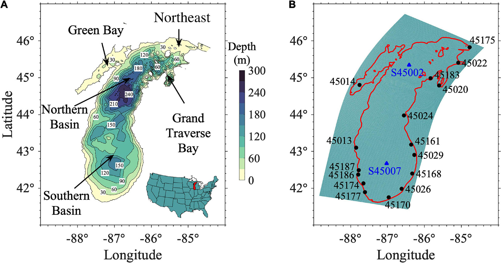
Figure 1. (A) Bathymetry and location of Lake Michigan in the United States. (B) Computational domain and curvilinear grid used for the wave hindcasting. The triangles indicate the locations of MetoOcean buoys S45002 and S45007 with long-term data from 1979 to 2020 and 1981 to 2020, respectively, while the circles indicate the locations of coastal buoys with short-term (later than 2010) data availability. Figures 1, 8, 9, 12, 14, 15 are produced following the guidance for colormap selection by Thyng et al. (2016).

While numerous studies have been performed to investigate the long-term wave statistics in oceanic and coastal regions (e.g., Tuomi et al., 2011, 2019; Camus et al., 2014; Bromirski and Cayan, 2015; Cheng et al., 2015; Wang et al., 2015; Niroomandi et al., 2018), there are only a few systematic lake-wide wave climate studies for the Great Lakes (e.g., Hubertz et al., 1991; Jensen et al., 2012), partly due to the limited long-term wave records. In Lake Michigan, all coastal buoys were deployed during 2010–2018 (Table 1). Long-term wave data with more than 30-year records, suitable for wave climate analysis (Trewin, 2007), are only available at two offshore National Data Buoy Center (NDBC) buoys [Station 45002 (hereafter S45002) and S45007, data available since 1979 and 1981, respectively], in the northern and southern basins (Figure 1B). In addition, the buoy data are not available during cold seasons (usually from December to April, Figure 2). Based on the data at the two offshore buoy stations, Olsen (2019) found that the measured yearly mean significant wave heights (H_s > 0.25 m from May to October) from 1981 to 2017 were decreasing at the rates of 1.5 mm/yr and 3.8 mm/yr at S45002 and S45007, respectively, with 95% confidence intervals using Theil-Sen regressions. Recently, Jabbari et al. (2021) investigated the trend of H_s in the months of August (1980–2018) at S45007 using linear regression and found an increasing trend of 2.4 mm/yr. In their data analysis, the missing wave data were filled using the empirical relation between H_s and the measured wind speed (Carter, 1982). The contradiction between Olsen (2019) and Jabbari et al. (2021) indicates that the trend of H_s in Lake Michigan may be nonlinear or even more complex. Additionally, the limited number of buoys (two for long-term analysis) is insufficient for accurate analysis of wave climate over the entire lake, especially under severe storm conditions (Mao et al., 2016).

TABLE 1

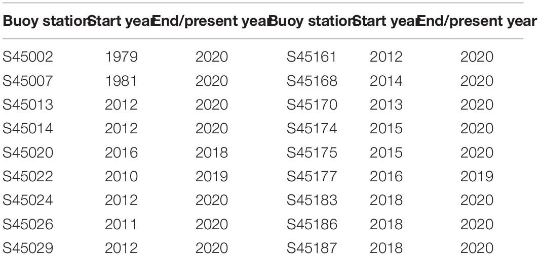
Table 1. Data availability for the buoys in Lake Michigan.

FIGURE 2

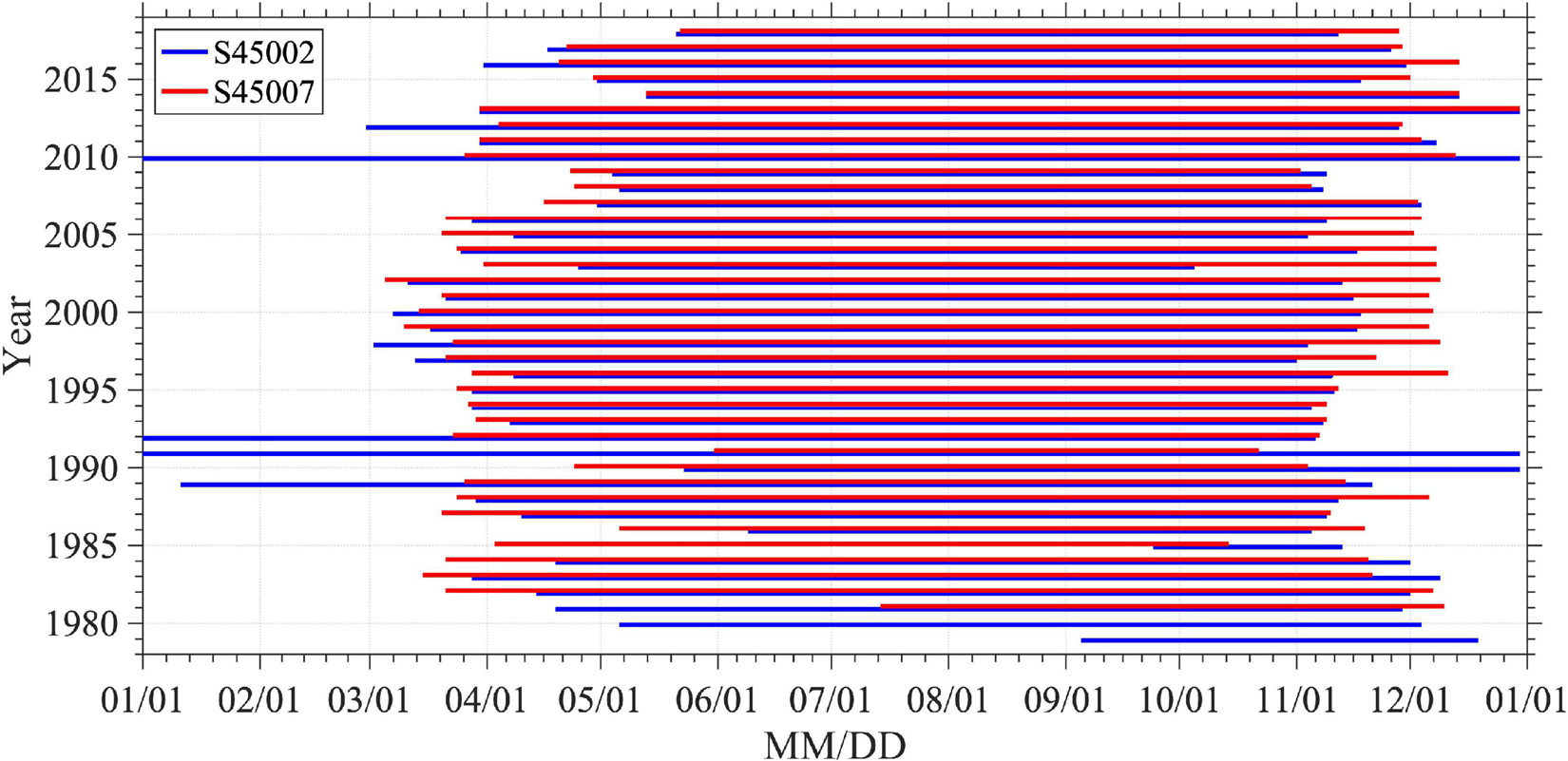
Figure 2. Data availability for buoys S45002 and S45007.

To fill the gaps of buoy data and develop the spatial distribution of wave climate, numerical models were often used (Caires and Sterl, 2005; Jensen et al., 2012; Bromirski and Cayan, 2015). Using the spectral wave model WAM Cycle 4.5.1C, the U.S. Army Corps of Engineers carried out long-term wave hindcasts for all the five Great Lakes under the Wave Information Studies (WIS) project (Hubertz et al., 1991; Jensen et al., 2012). For Lake Michigan, the WIS provided wave hindcasts from 1979 to 2017 at 490 nearshore stations around the lake. With the WIS data at nearshore stations, Olsen (2019) found there were only a few stations in the southwest and two stations in the southeast of the lake that had statistically significant decreasing trends for the yearly mean of H_s > 0.25 m while there were no significant trends for the majority of WIS stations. On the other hand, using the 32-year DWAVE model (Resio and Perrie, 1989), an earlier model version used in the WIS project from 1956 to 1987, Meadows et al. (1997) established a correlation between the Great Lakes water levels and incident wave energies, having hypothesized that they were associated with large-scale shifts in atmospheric storm tracks. This again indicates the complex changes in wave climate influenced by regional climate change.

Since the study of Meadows et al. (1997), the water level of Lake Michigan in the past four decades has shown strong interannual variability. The lake level declined from a high water level in 1987 to a level below the long-term mean in 1999 and remained very low (setting an all-time low in January 2013) for more than a decade until 2014. Since then, the lake level has increased rapidly by ∼2 meters in 6 years. In 2020, the water level continually broke the monthly record high through January to August. Meanwhile, Lake Michigan has experienced some of the biggest waves with wave height reaching 6.5 m during fall storm events in the past decade (e.g., Sep 30, 2011,¹ October 31, 2014,² March 6, 2020³). Additionally, the ice coverage during winter has significantly reduced in the Great Lakes (Assel et al., 2003; Wang et al., 2012) in response to regional warming trends. As ice coverage affects the wind waves by reducing wind stress and dissipating wave energy (Bennetts et al., 2010; Doble et al., 2015; Sutherland and Rabault, 2016; Kohout et al., 2017; Voermans et al., 2019; Yiew et al., 2019; Bai et al., 2020), reduced ice coverage is expected to favor the wave growth. The combined impacts of these factors on the wave climate in Lake Michigan have not been fully understood.

The objective of this study was to investigate the response of long-term wave climate for the entirety of Lake Michigan to the changes in regional climate factors using a numerical wave model. The model was validated against the measured wave data from offshore and coastal MetOcean buoys. The validated model was then applied to investigate the spatial and seasonal characteristics of the wave climate in Lake Michigan with a focus on wave climate change. To investigate the long-term changes in H_s, the validity of conventional linear regression used in previous studies was examined. Furthermore, after removing the seasonal and annual variability with the 10-year moving average, we identified the regime shifts of H_s and its correlations with wind speed, water level, and ice cover. Finally, case studies were conducted to explore the impact of decreasing ice cover on the wave climate.

Materials and Methods

Data

Various datasets were used in this study for data analysis, model input, and model validation. The data for SWAN model inputs included hourly surface wind forcing and daily ice cover. The hourly surface wind forcing was obtained from the Climate Forecast System Reanalysis (CFSR)⁴ dataset with a spatial grid resolution of ∼0.3 degree for 1979–2010 and the upgraded Climate Forecast System Version 2 (CFSv2)⁵ dataset with a higher spatial resolution of ∼0.2 degree, which is archived as an extension of CFSR and available from 2011 to present at the National Centers for Environmental Prediction (NCEP) (Saha et al., 2010, 2011). CFSR is a global, high-resolution, coupled atmosphere-ocean-land surface-sea ice system, with the assimilation of satellite radiances and all available conventional and satellite observations. Analysis of the CFSR output indicates the product is far superior in most respects to the reanalysis of the mid-1990s (Saha et al., 2010, 2011), and has shown good performance over the Great Lakes regions (Jensen et al., 2012; Xue et al., 2015). The daily ice cover on Lake Michigan was obtained from the Great Lakes Ice Cover Database,⁶ which includes the Great Lakes Ice Atlas⁷ for the period 1973–2002, with addendums for 2003 through present.

Both the daily ice cover data described above and the monthly lake-wide average water levels were analyzed to understand their impacts on the wave climate. Monthly lake-wide average water levels were obtained from the Great Lakes dashboard of NOAA Great Lakes Environmental Research Laboratory.⁸ These lake-wide averages were derived based on a selected set of U.S. and Canadian station data as determined by the Coordinating Committee on Great Lakes Basic Hydraulic and Hydrologic Data, which represents the best estimates of the lake-wide mean water levels.

Lake-wide buoy observations were used for the SWAN model validation. Surface conditions across Lake Michigan were well documented with two offshore buoys (MetOcean buoys operated by the NDBC of NOAA) and sixteen coastal buoys (operated through the Great Lakes Observing System (GLOS) with funding from the Integrated Ocean Observing System (IOOS) of NOAA). The two offshore MetOcean buoys are NDBC S45002 and S45007. S45002 is a 3-meter discus buoy with Self-Contained Ocean Observing Payload (SCOOP), which provides wind speed, wind direction, wind gusts, wave height, dominant wave period, average wave period, mean wave direction, and a variety of other air/sea measurands hourly. NDBC S45007 is a 2.3-m foam discus buoy also with SCOOP and similarly reports hourly. The sixteen coastal buoys operated by a variety of universities and other GLOS partners are primarily TIDAS 900 buoys.⁹ These buoys consist of a 1.1 m-diameter conical hull with a six-degree-of-freedom wave sensor providing at a minimum, the same suite of sensors as the NDBC buoys, however, at a much higher rate of reporting to capture the rapid change characteristics of coastal regions. Equipped with the SeaView Systems 603 wave sensor,¹⁰ TIDAS buoy motions were recorded for 17.06 min at a sample rate of 2 Hz for a time series sample of 2048 observations. Buoy wave parameters were reported at 20-min intervals and available through GLOS and NDBC.

Model Configuration

Prevalent numerical models for wave hindcast are the third-generation spectral wave models including Wave Modeling (WAM, WAMDI Group, 1988), WAVE-WATCH III (Tolman, 1991), TOMAWAC (Benoit et al., 1997) and Simulating Wave Nearshore (SWAN, Booij et al., 1999). In this study, the SWAN model was used to investigate the spatiotemporal changes of wave climate. SWAN is a third-generation spectral wave model developed at Delft University of Technology that computes random, short-crested wind-generated waves in coastal regions and inland waters.¹¹ It solves the evolution equation of wave action density $N(\overrightarrow{x},t;\mathrm{\sigma },\mathrm{\theta })$ in space $\overrightarrow{x}$ and time t over frequency σ and wave direction θ,

$$\frac{\partial N}{\partial t}+{\nabla }_{\overrightarrow{x}}\cdot \left[\left({\overrightarrow{c}}_g+\overrightarrow{U}\right)N\right]+\frac{\partial c_{\mathrm{\sigma }}N}{\partial \mathrm{\sigma }}+\frac{\partial c_{\mathrm{\theta }}N}{\partial \mathrm{\theta }}=\frac{S_{tot}}{\mathrm{\sigma }},(1)$$

where ${\overrightarrow{c}}_g$ is the group velocity, $\overrightarrow{U}$ is the mean current. The quantities c_σ and c_θ are the propagation velocities in spectral space (σ, θ), and S_tot is the source term. In (1), the left-hand side describes the wave kinematics, and the right-hand side accounts for various wave energy sources and sinks, including wave generation by wind, wave decay due to whitecapping, bottom friction, and depth-induced wave breaking, as well as energy redistribution through nonlinear wave-wave interactions. Recognized as a reliable coastal community wave model, SWAN has been widely applied for wave hindcasting and forecasting (Rogers et al., 2003, 2007) for the Great Lakes (Anderson et al., 2015; Mao et al., 2016; Huang et al., 2021) and coastal oceans (Dietrich et al., 2011; Huang et al., 2013; Cheng et al., 2015; Xie et al., 2016; Niroomandi et al., 2018; Xie et al., 2019).

A curvilinear grid mesh was applied in the SWAN simulation, which consists of 181 × 496 grid cells with a grid resolution of ∼1 km (Figure 1B). The spectral domain was discretized into 12 directions with 30-degree intervals and 32 frequency bands from 0.0521 to 1.0 Hz. The default values of the parameters in SWAN model were employed. The model was driven by hourly surface wind forcing from the CFSR and CFSv2.

To address the effects of ice coverage on wind-generated waves, a common technique is to mask the mesh cell with land when the local ice coverage exceeds a threshold value (e.g., Hubertz et al., 1991; Bennington et al., 2010; Tuomi et al., 2011; Anderson et al., 2015). This was realized through bathymetry modifications by changing the ice-covered areas to land points (Tuomi et al., 2019). The temporal variations of daily ice cover were from the NOAA Great Lakes Ice Cover Database described in section “Data”. Following the study in Great Lakes by Anderson et al. (2015), the value of 30% was selected as the threshold value used in this study, i.e., the wave energy was assumed to be totally dissipated where the ice coverage exceeds 30% at a given model grid cell.

Model Validation

A 42-year long hindcasting was performed from 1979 to 2020. The model results were compared with the measured significant wave heights (H_s) and peak wave period (T_p) at 18 buoy stations in Lake Michigan (Figure 1B). Among these buoys, S45002 (45.344N, 86.411W) was installed in the northern basin in 1979, while S45007 (42.674N, 87.026W) in the southern basin in 1981. The other 16 buoys were deployed in shallower water along the coast within less than 7 km to the shoreline in the last 10 years (Figure 1B and Table 1). Since the buoys were removed during cold seasons (usually from December to April), wave measurements were not available for this period. The buoy data availability is summarized in Table 1 with more details for the two long-term buoy records at S45002 and S45007 shown in Figure 2.

The performance of the model was assessed using the following four statistical error measures: Bias, Root Mean Square Error (RMSE), Scatter Index (SI), and R². The bias is the difference between the calculated and measured mean values and given by

$$Bias=\overline{Y}-\overline{X},(2)$$

where $\overline{Y}={\sum }_{i=1}^N{Y}_i/N$ is the mean of the calculated values Y_i (i = 1, 2..N) from the model and $\overline{X}={\sum }_{i=1}^N{X}_i/N$ is the mean of the measured values X_i (i = 1, 2..N) from observation with sample size of N. The RMSE is calculated using the following formula,

$$RMSE=\sqrt{\frac{1}{N}\sum _{i=1}^N{\left(Y_i-X_i\right)}^2}.(3)$$

The SI is defined as the normalized RMSE by the measured mean value and given by Lin et al. (2002)

$$SI=\frac{RMSE}{\overline{X}}.(4)$$

The R² is the coefficient of determination defined as

$$R^2=1-\frac{{\sum }_{i=1}^N{\left(Y_i-X_i\right)}^2}{{\sum }_{i=1}^N{\left(X_i-\overline{X}\right)}^2}.(5)$$

The comparisons between the calculated and measured H_s and T_p were conducted for all the available buoy data from 1979 to 2020. For the purpose of demonstration, direct model-data comparisons of H_s and T_p based on hourly results for 2020 at the two offshore buoys and 12 coastal buoys (no data available from the other four coastal buoys) are shown in Figures 3, 4, respectively. Such comparisons for other years are presented in the (Supplementary Figures 1–8). The model showed consistent performance over the entire simulation period. As shown in Figure 3, the hourly wave heights oscillated in a range of 0–3 m during the year, with stronger waves generally after mid-September. Substantial spatial variability was shown across the lake. The largest wave heights were observed offshore and exceeded 2.8 m at S45002 and S45007. Coastal waves were generally weaker, yet strong waves with H_s greater than 2 m occurred on the east coast at S45024. In other coastal regions, H_s was generally below 2 m, and the H_s along the southwest coasts at S45186 was particularly small with H_s less than 1m in most of the year.

FIGURE 3

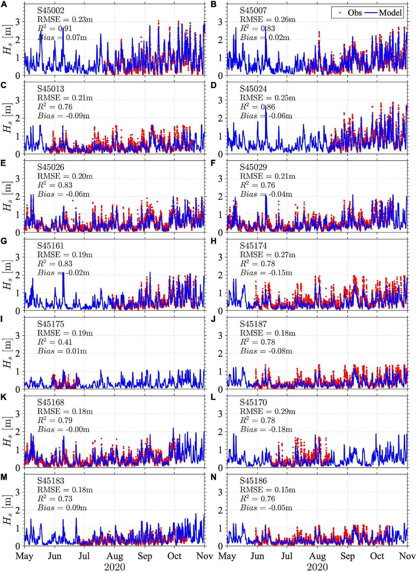
Figure 3. Comparisons between the modeled and measured significant wave heights (H_s) at buoys (A) S45002, (B) S45007, (C) S45013, (D) S45024, (E) S45026, (F) S45029, (G) S45161, (H) S45174, (I) S45175, (J) S45187, (K) S45168, (L) S45170, (M) S45183, and (N) S45186 for the most recent year 2020 (Comparisons for every other year are shown in Supplementary Figures 1–4).

FIGURE 4

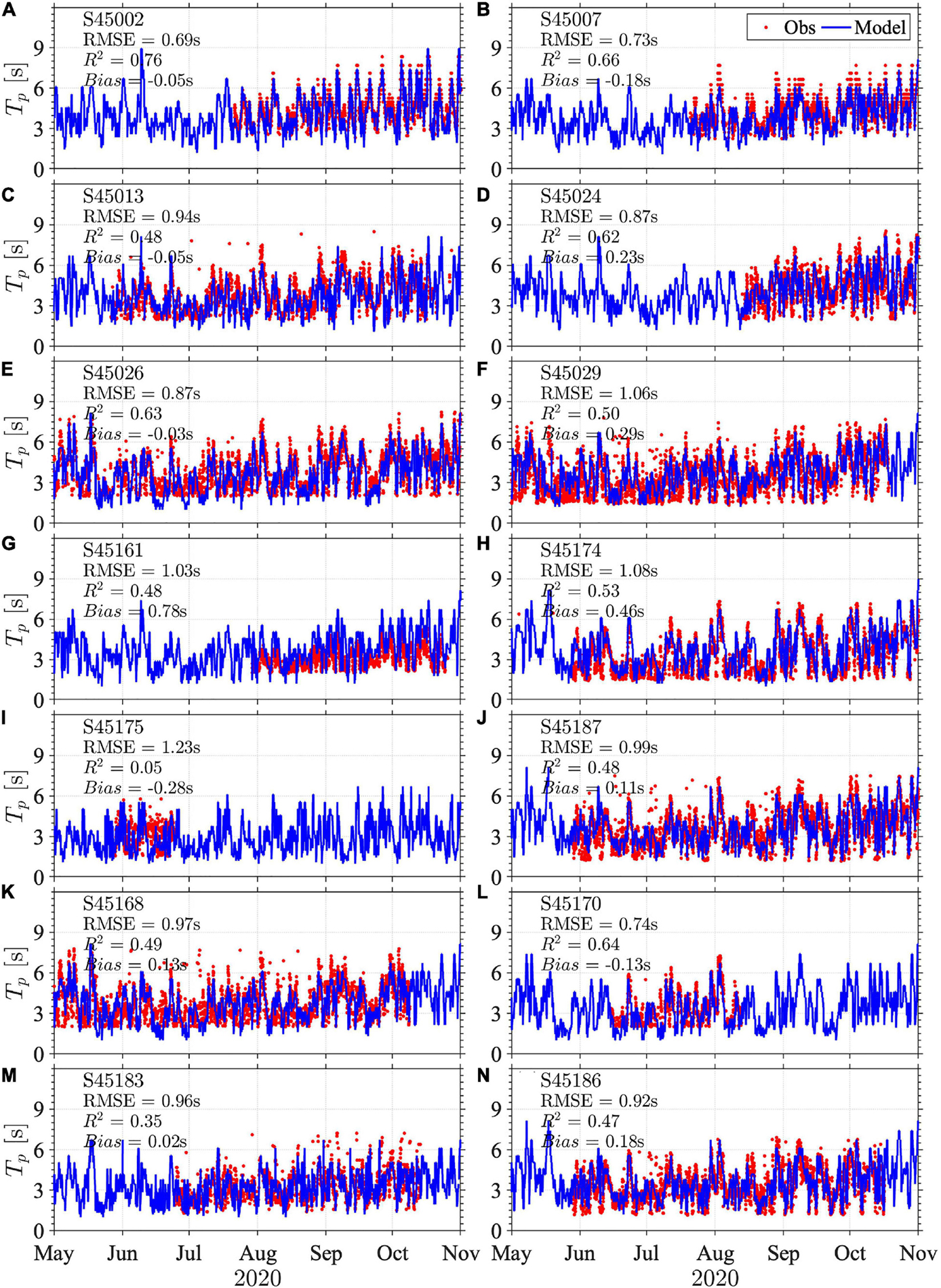
Figure 4. Comparisons between the modeled and measured peak wave period (T_p) at buoys (A) S45002, (B) S45007, (C) S45013, (D) S45024, (E) S45026, (F) S45029, (G) S45161, (H) S45174, (I) S45175, (J) S45187, (K) S45168, (L) S45170, (M) S45183, and (N) S45186 for the most recent year 2020 (Comparisons for every other year are shown in Supplementary Figures 5–8).

The model captured the spatiotemporal pattern of the wave characteristics (Figure 3) very well. Particularly in offshore regions, the modeled H_s agreed well with the measurements at S45002 and S45007 with R² = 0.91 and R² = 0.83, respectively. For coastal waves, the model also showed a close agreement with observation with R² values between 0.73 and 0.86 for all but two buoys (S45175 and S45186). The results showed the model explained at least 70% of the variability of the observed data around its mean. In addition, the model showed small RMSE (0.15–0.29 m) and bias (± 0.09 m) except for S45174 and S45170 with bias of –0.15 m and –0.18 m, respectively, which is likely to be caused by the underestimation for large waves. Comparisons of T_p were generally less desirable but still showed a reasonably good agreement (R² = 0.76 and R² = 0.66) at the two long-term record offshore buoys S45002 and S45007 (Figures 4A,B). At coastal buoys, the model-data comparisons of T_p were reasonably well, except for the comparison at S45175 (Figure 4I). The RMSE for T_p comparison was less than 1.08 s except for S45175 (RMSE = 1.23 s), where available observation data were very limited. Additionally, the results also showed small biases of less than 0.30 s except for S45161 and S45174, which had larger biases of 0.78 s and 0.46 s, respectively.

Long-term wave hindcasting for annual mean H_s, 90th percentile H_s, and 99th percentile H_s from 1979 to 2020 was evaluated (Figure 5). For appropriate comparisons, the annual statistics for buoy measurements and model results were calculated for the same time period based on the buoy data availability (Figure 2). This is referred to as Type M statistics in Tuomi et al. (2011), i.e., statistics calculated only from the time coinciding with the measurements. Results have shown that the model accurately captured the interannual variability of significant wave height for its mean and 90th percentile values. For example, in the northern basin (S45002), both mean and 90th percentile wave heights showed a continuous increase during 1980–1985, followed by a relatively large decrease in wave heights in 1986 before the wave heights increased again until 1990 and decreased throughout 1995. In addition, the 90th percentile H_s in the northern basin in 2007 was noticeably higher than previous and following years, which has also been accurately captured by the model. The model generally underestimated the extremely high waves (i.e., 99th percentile H_s) before 2010, particularly in the years of 1995, 2001, and 2007. Nonetheless, the model performed well in capturing the 99th percentile wave heights after 2010. This is likely due to the improved wind forcing data from the CFSv2 available from 2011.

FIGURE 5

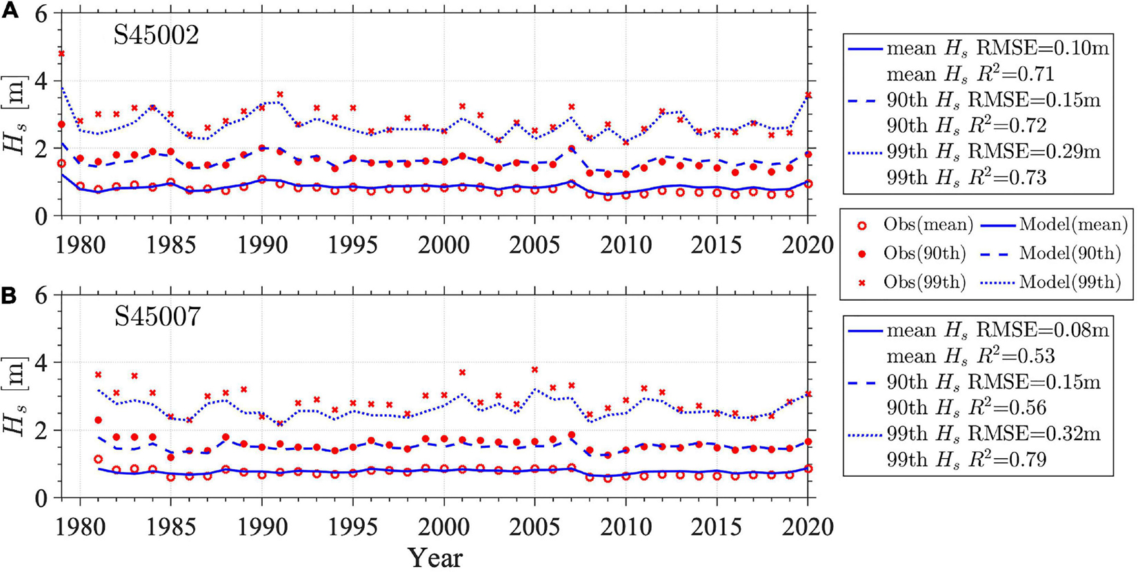
Figure 5. Comparisons between calculated and measured annual mean, 90th percentile, and 99th percentile significant wave heights (H_s) at buoy stations (A) S45002 from 1979 to 2020 and (B) S45007 from 1981 to 2020 based on Type M statistics.

In addition to the statistics of annually averaged wave characteristics, the scatter plots of the hourly H_s were also assessed across the lake (Figure 6, Type M statistics). Six representative sampling locations were selected, including two offshore buoys: northern basin (S45002) and southern basin (S45007), four coastal buoys that represent northeast coast (S45022), east coast (S45024), southeast coast (S45026), and southwest coast (S45186). The model explained the variability of data well, indicated by a high R² value (0.66–0.82). The SI ranged between 0.3 and 0.5, which is also similar to the SI ranges reported in other wave modeling evaluations (Lin et al., 2002; Anderson et al., 2015; Vieira et al., 2020). More importantly, the Quantile-Quantile (Q-Q) plots (magenta crosses) show that wave height distributions from model and observations were highly consistent in the offshore basins, northeast, and east coasts as Q–Q plot approximately lied close to the line y = x. In the southeast and southwest coasts, the model was able to accurately reproduce weak wave conditions (i.e., H_s < 1 m) but underestimated large waves (e.g., 99th percentile H_s), particularly at S45026.

FIGURE 6

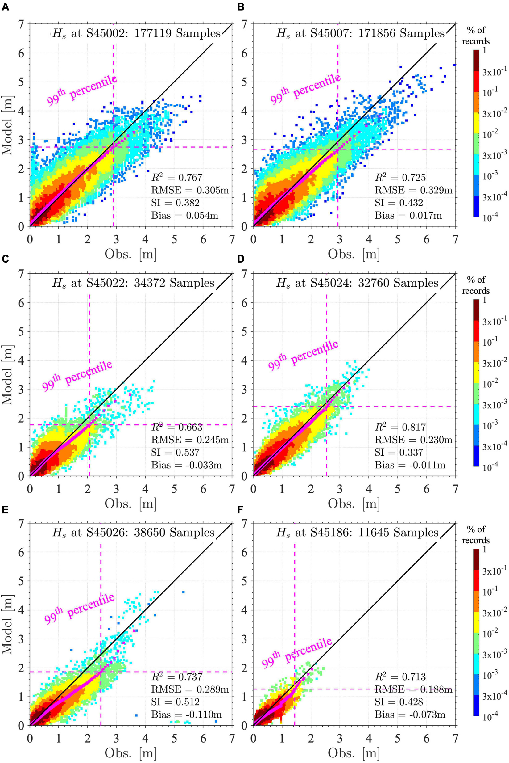
Figure 6. Scatter plots of model and measured significant wave heights (H_s) at offshore buoys (A) S45002 and (B) S45007 as well as coastal buoys (C) S45022, (D) S45024, (E) S45026, and (F) S45186. The percentages of data are calculated within a 0.1×0.1 m² for H_s and denoted by contour map. The Quantile-Quantile (Q-Q) plot is overlaid using magenta crosses with vertical and horizontal magenta dashed lines indicating the 99th percentile value. The R², root-mean-square-error (RMSE), Scatter Index (SI), and Bias are shown in the legend based on Type M statistics.

Results and Discussion

Wave Climate in Lake Michigan

There are several ways to calculate wave statistics in the presence of a seasonal ice cover as laid out in detail by Tuomi et al. (2011). For example, we have used Type M statistics in section “Model Configuration” for model validation. Other main types of statistics described in Tuomi et al. (2011, 2019) include Type I (statistics with ice time included when H_s = 0 m), Type F (ice time excluded completely from the calculations), Type N (hypothetical no-ice conditions). In the following sections, we use the type I analysis for H_s unless noted otherwise. Namely, wave analysis performed at any given location utilizes the entire 42-year simulation results including the ice time with H_s = 0 when the local ice cover exceeds the threshold value of 30%. In such a way, it allows us to directly assess the impact of ice cover change on the wave climate.

To understand the seasonality and spatial variability of wave height, the modeled 42-year (1979–2020) mean lake-wide average significant wave height H_s, 90th percentile, and 99th percentile for each month, respectively, are provided in Figure 7. It is clear that the wave height variability closely aligned with the wind speed at 10 m height (U₁₀) except in the mid ice season. Winds were the strongest in January but the presence of ice cover reduced the wave height compared to December. In February, decreasing U₁₀ and increasing ice cover both helped reduce waves. However, in March and April, decreasing U₁₀ and decreasing ice cover offset their negative and positive impacts on wave growth, leading to an insignificant change in H_s. With the disappearance of ice after April, the wave height dropped rapidly from May to August in response to the decreasing wind during summertime. The increasing wind in the fall enhanced wave development, and the wave height reached the annual peak in December when the winds became strong in wintertime and ice had yet to develop.

FIGURE 7

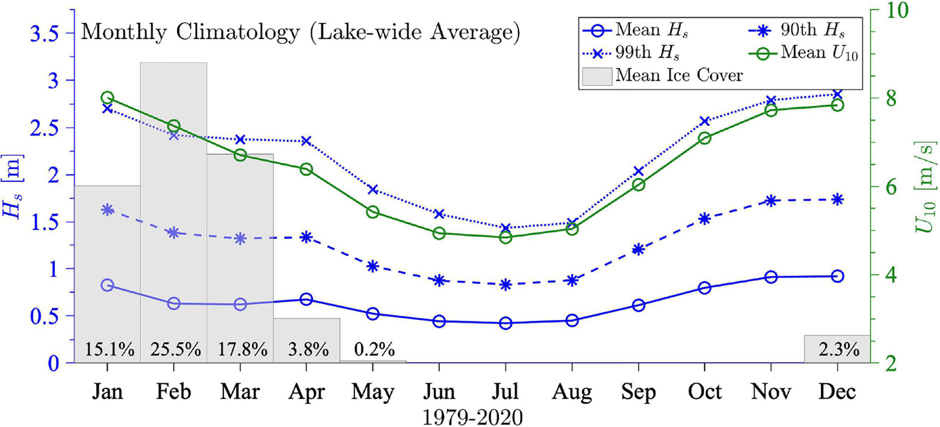
Figure 7. Monthly climatology of the lake-wide average of significant wave height (H_s) based on Type I analysis in Tuomi et al. (2011) were performed here with the wind speed (U₁₀) at 10 meter height from the model simulations over 1979–2020. Barchart presents monthly ice coverage percentage.

Since the buoy data were usually not available from December to April, the observation data provided an incomplete picture of the wave characteristics and would underestimate the annual wave conditions. The model results are, therefore, essential to provide a comprehensive understanding of the wave climate in the entire lake and throughout all seasons. This was depicted by comparing the wave patterns averaged over the ice-free season, the ice season, and the entire year (Figure 8). We note that the ice season in this work is defined as December to April, which is based on the monthly climatology of ice cover in Figure 7. It is possible that ice may not be present at some location during ice season or may be present during the ice-free season over the 42-year simulation time. This should not be confused with the time of ice cover at a given specific location. All results in Figure 8 are based on the Type I analysis. Waves were stronger offshore than along coastal regions. On a close look, meridional differences in mean H_s between the northern and southern basins were noticeable during the ice season, with stronger waves in the southern basin resulting from the dominant northwesterly wind during the winter (Figure 8A2). On the other hand, the zonal difference in large waves (i.e., 99th percentile H_s) between west and east became more evident, showing stronger waves in the eastern part of the lake (Figures 8C1–C3).

FIGURE 8

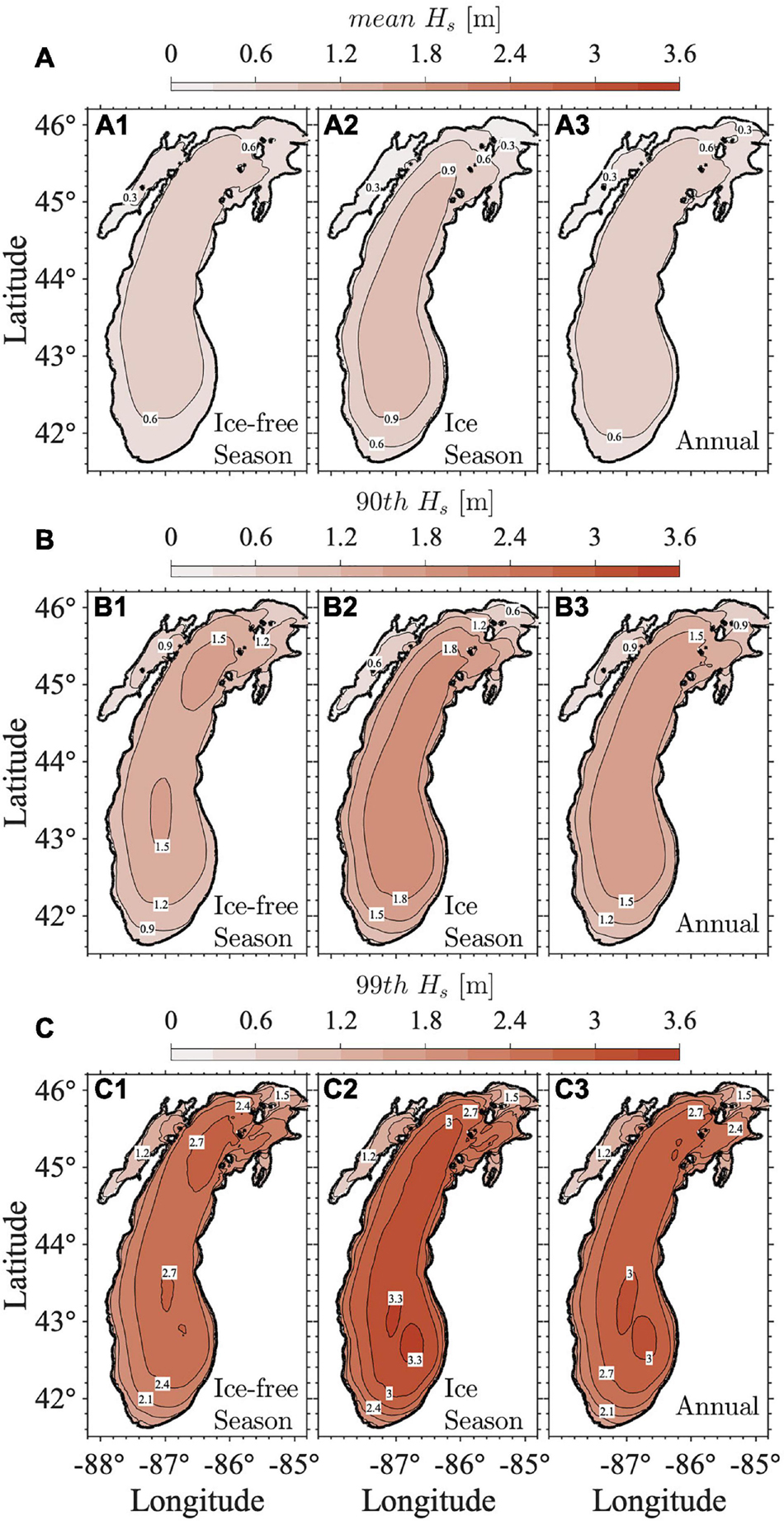
Figure 8. The SWAN modeled 42-year (1979–2020) (A) mean, (B) 90th percentile, and (C) 99th percentile significant wave height (H_s) in (A1,B1,C1) ice-free season (May–November), (A2,B2,C2) ice season (December–April), and (A3,B3,C3) the whole year based on Type I statistics.

Wave Regime Shift

To address whether linear trends of wave climate existed across the lake that may facilitate the wave climate projection, we investigated the spatial pattern of the trends of H_s for the entirety of Lake Michigan. Linear regression analyses of H_s were conducted regarding the mean, 90th percentile, and 99th percentile of annual averaged H_s for the past 42 years (1979–2020). The MATLAB function Regstats was used to obtain all the regression coefficients based on the least square estimator and their 95% confidence intervals. Regions with a statistically significant trend at 95% confidence level are marked in Figure 9. The mean H_s and 90th percentile H_s showed a statistically significant increase in some small areas in the northeast, east, and southeast of the lake. For the 99th percentile H_s, a statistically significant increase existed only in smaller regions in the northeastern and eastern coasts. In contrast, a downward trend was observed within a band from the west coast to the south basin. The results have shown that there was no simple linear trend of long-term H_s change for the majority (> 90%) of the lake. Similarly, we applied the same linear trend analysis to H_s of successive January(s), February(s), …, December(s) of the 42 years, respectively. The results were consistent with Figure 9 that no linear trend could be established for most areas of the lake.

FIGURE 9

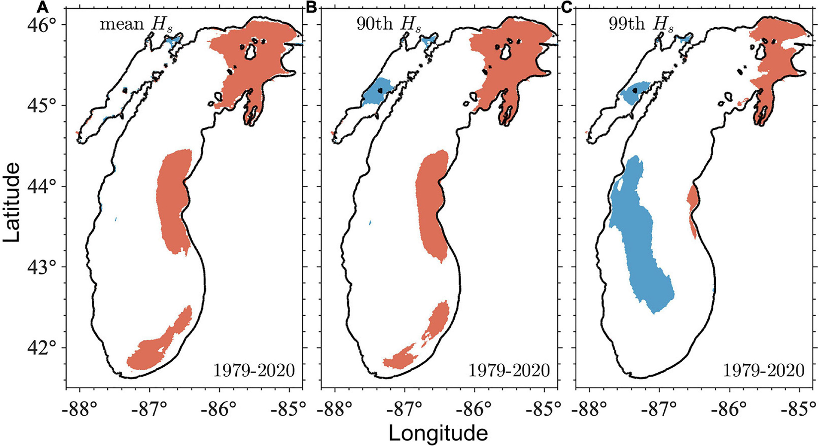
Figure 9. Linear trends of the (A) annual mean H_s, (B) annual 90th H_s, (C) annual 99th percentile H_s for 1979–2020. Only locations where the trends are statistically significant at 95% confidence level are shaded based on Type I statistics. Red (blue) color indicates a trend of increase (decrease).

The above analysis suggests the inadequacy of linear trend analysis used in previous studies (Olsen, 2019; Jabbari et al., 2021). It also reinforces the complexity of wave climate in Lake Michigan. A 10-year trailing moving mean was therefore applied to H_s to remove seasonal and annual variability, focusing on long-term wave patterns (Figure 10). Simulated waves at all buoy locations suggest there was no clear trend and instead, regime shifts were identified. Specifically, there were trends of increasing H_s around 2010–2020 along with rising water levels at 14 out of the 16 representative buoy stations, except S45013 and S45186 at the southwest coast, where the increasing trends after 2010 were less certain. However, it should be noted that S45187 and S45174 were also located on the southwest coast and showed clear trends of increasing wave height. Furthermore, all stations showed low H_s around the period of 2000–2010 (coincident with low lake levels). In addition, 14 stations (except S45020, S45022) illustrated a downward trend around 1990–2000. These patterns resembled the annual water level change in the region with the correlation coefficients greater than 0.8 at five stations, between 0.7 and 0.8 at two stations, and between 0.6 and 0.7 at four stations (Figure 10). Increasing H_s possibly reflected increases in storm intensity and frequency, preceding the rising lake-wide water level.

FIGURE 10

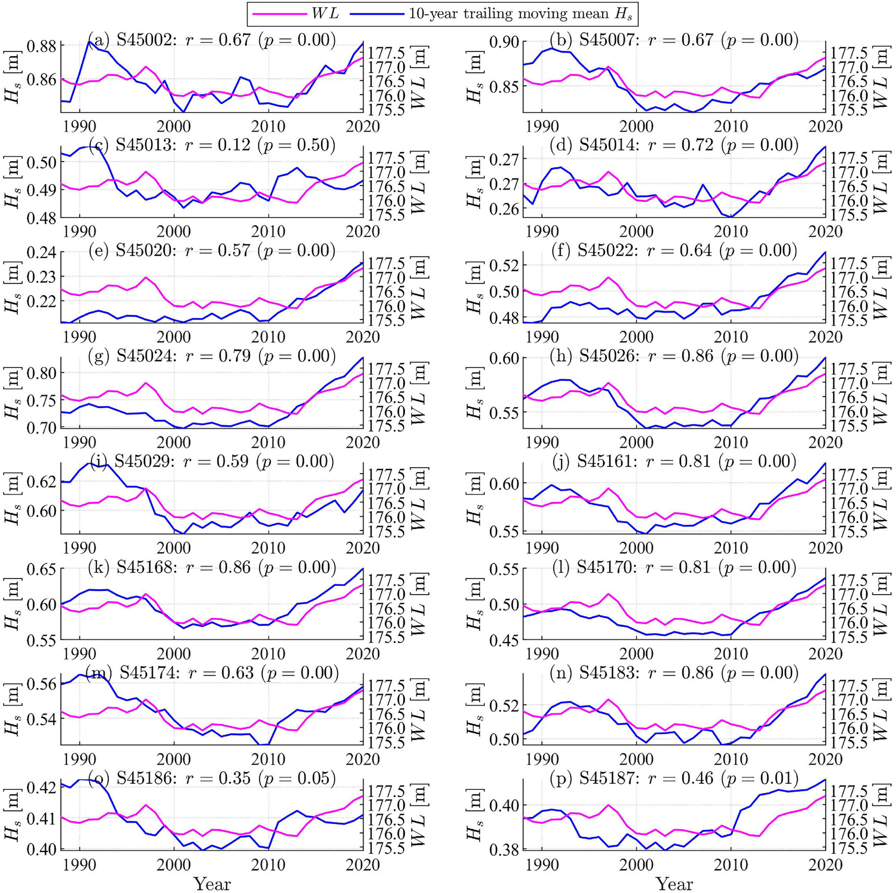
Figure 10. Time series of 10-year trailing moving mean of significant wave height (H_s) associated with annual mean water level (WL) at 16 selected representative stations based on Type I statistics.

Water level changes do not directly influence wave height significantly, except very shallow nearshore regions where the water level change would impact the wave shoaling and breaking. However, results in Figure 10 have revealed the correlation between changes in water level and wave height across the lakes in both offshore and coastal regions that are further away from nearshore zones. The correlation between water level and wave height does not suggest any causal relationship between the two variables. Instead, such correlation suggests they were both influenced by atmospheric and regional climate patterns. On one hand, the wave height is known to be primarily controlled by local wind speed, duration, and fetch in the Great Lakes (Pore, 1979; Donelan et al., 1985), while in coastal oceans swells also play an important role (Aboobacker et al., 2011; Sabique et al., 2012; Wandres et al., 2020). The H_s and wind speed at a 10 m height showed a strong correlation with a correlation coefficient of r≥0.90 at 12 out of the 16 stations (not shown). On the other hand, the primary drivers of water levels in the Great Lakes are runoff, over-lake precipitation, connecting channel flow, and evaporation (Deacu et al., 2012). Regional climate assessment showed that more intense storms due to hydrologic intensification have been observed in the Great Lakes region in the past decades. The amount of precipitation falling in the heaviest 1% of storms increased by 35% in the Great Lakes region from 1951 through 2017 (USGCRP, 2017). Therefore, the changing pattern in storms, which influences waves (instantly through increased wind stress on the surface) and water levels (following, with a lag through precipitation and runoff), is likely to be a driving factor responsible for the observed correlation between the wave height and water level.

With a changing regional climate, the Lake Michigan water level has shown three regimes in the past four decades with a high water level between 1980 and 1998, remained an extremely low water level for more than a decade during 2000–2013, and followed by a drastic and rapid increase (water level increased by 2 m within 6 years) during 2014–2020 (Figure 11). The shifts among these three regimes occurred around 1998 and 2014, corresponding to two strong El Niño events, i.e., the 1997–98 and 2014–16 events. To further validate the hypothesis on coherent patterns of the waves, water level, and their possible connection to the regional climate change including storminess and ice reduction; we analyzed the differences in large waves (99th percentile H_s) during these three regimes defined by water level change, as they are a more suitable indicator of storm impacts than mean waves height. The changes in 99th percentile H_s from the first regime (1979–1998) to the second regime (1999–2013) and from the second regime (1999–2013) to the third regime (2014–2020) are shown in Figure 12.

FIGURE 11

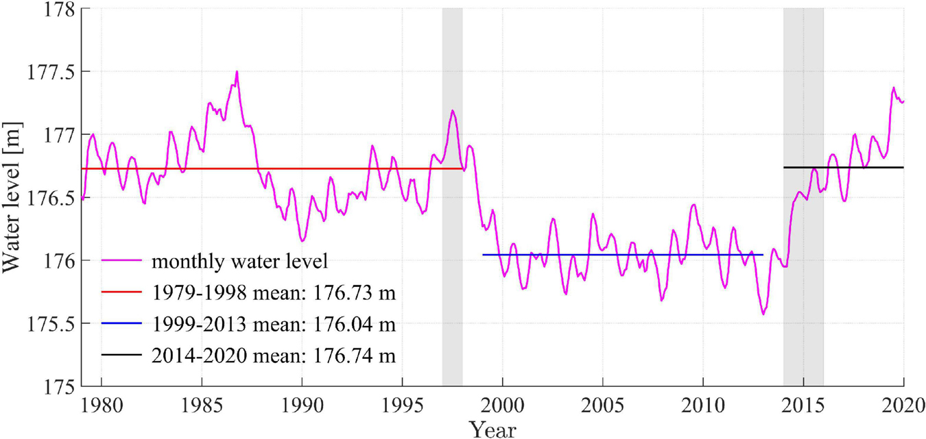
Figure 11. Monthly water level from 1979 to 2020 showing three regimes with high water level in regime 1979–1998, low water level in regime 1999–2013, and recently increasing water level in regime 2014–2020. The shaded gray patches indicate two strong El Niño events, i.e., the 1997–98 and 2014–16 events.

FIGURE 12

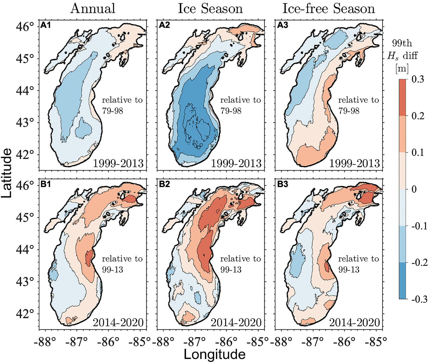
Figure 12. Difference in 99th percentile H_s based on Type I statistics between the first period (1979–1998) and the second period (1999–2013) for the whole year (A1), ice season (A2), ice-free season (A3). Difference in 99th percentile H_s between the second period (1999–2013) and the third period (2014–2020) for the whole year (B1), ice season (B2), ice-free season (B3).

From the period of 1979–1998 to the period of 1999–2013, the wave height (99th percentile H_s) averaged over each period, decreased by 0.1–0.3 m in the majority of the lake (Figure 12A1). This is consistent with the shift from high water to low water levels (Figure 11). The exception is in the northernmost region where the wave height increased by < 0.1 m due to decreasing ice cover, which is discussed in the following section. During the ice season, a similar pattern of wave change was observed (Figure 12A2), with changes in the magnitude of H_s becoming more drastic. Unlike the pattern during ice season, the changing pattern during the ice-free season showed a somewhat opposite pattern with an increase in wave height in the eastern lake and southern lake while a decrease was observed in the western and northern lake (Figure 12A3). These results suggest the complexity of spatiotemporal patterns of storm changes, indicating the possibility of declined winter storms and increased summer storms during this period. However, the annual wave pattern is significantly influenced by the wave pattern during the ice season, highlighting the essential role of winter wave conditions in wave climate.

In contrast, from 1999–2013 to 2014–2020, wave heights increased in most regions of the lake by 0.1–0.3 m, including the entire northern lake and the eastern part of the southern lake (Figure 12B1). In addition, the increases in wave heights during the period of 2014–2020 were consistent across the ice season, ice-free season, and annual average, showing an apparent increase in wave heights that were well aligned with rapid water level rise. This reinforces the hypothesis of coherent patterns of the waves, water level, and their connection to more frequent and intensified storms observed in the Great Lakes in the past.

Impact on Wave Extreme Value

In this section, we made an attempt to examine if the changes in wave climate can be detected in wave height extreme value and its impact on design wave heights corresponding to different return periods. Independent events were selected from the continuous time series of H_s using the peaks-over-threshold (POT) method. To ensure the independence of events, the selected events were recommended at least 48 h apart (Caires and Sterl, 2005; Aarnes et al., 2012; Anderson et al., 2015; Velioglu Sogut et al., 2018). Following Méndez et al. (2006) and Niroomandi et al. (2018), a minimal time interval of 72 h between events was adopted in this study. The threshold value for individual wave events was set as 3 m, which is comparable to the 99th percentile for H_s in the offshore station 45002 during the 42-year simulation. Sensitivity analysis was also conducted by selecting a threshold of 3.3 m (99.5th percentile), results remained nearly the same. The return period analysis was conducted with the selected wave events by fitting the Generalized Pareto distribution (GPD). The cumulative distribution function for GPD was given by Coles (2001),

$$F\left(y\right)=\{\begin{array}{c}\hfill 1-{\left(1+\frac{\xi y}{\mathrm{\sigma }}\right)}^{-\frac{1}{\xi }},\mathrm{if}\xi \ne 0\hfill \\ \hfill 1-\exp \left(-\frac{y}{\mathrm{\sigma }}\right),\mathrm{if}\xi =0\hfill \end{array},(6)$$

where y values are threshold excesses, σ is the scale parameter, and ξ is the shape parameter. The parameters σ and ξ were obtained by maximum likelihood estimates. Then, the return level was estimated by Coles (2001),

$$H_{s,N}=\{\begin{array}{c}\hfill \mathrm{\mu }+\frac{\mathrm{\sigma }}{\xi }\left[{\left(N{n}_y\right)}^{\xi }-1\right],\mathrm{if}\xi \ne 0\hfill \\ \hfill \mathrm{\mu }+\mathrm{\sigma }\ln (N{n}_y),\mathrm{if}\xi =0\hfill \end{array},(7)$$

where μ is the threshold, n_y is the average number of the POT selected events per year, and N is the return period in years.

Design wave heights at the offshore buoy location S45002 corresponding to different return periods were calculated repeatedly using simulation data from three periods (Figure 13), namely, Period I: 1979–1998 (regime 1); period II: 1979–1998 plus 1999–2013 (regime 1 plus regime 2), and period III: 1979–1998 plus 2014–2020 (regime 1 plus regime 3). The 100-year return level of H_s during period I was estimated to be 6.05 m. Using the data in period II, the 100-year return level of H_s reduced slightly to 5.87 m, which reflects the impact of the reduced H_s during regime 2 as discussed before. Similarly, with the data in period III, the 100-year return level of H_s was elevated to 5.98 m. This again reflects the increased H_s during regime 3. Consistently, the events exceeding the threshold decreased during period II and increased during period III (Figure 13). However, these estimated 100-year return levels only vary moderately (<2% variation relative to the mean of these values = 5.96 m) using data from the three periods, suggesting the robustness of the estimates. It also suggests that the changes in wave climate during the past four decades have had no significant impact on design wave weight and extreme value analysis.

FIGURE 13

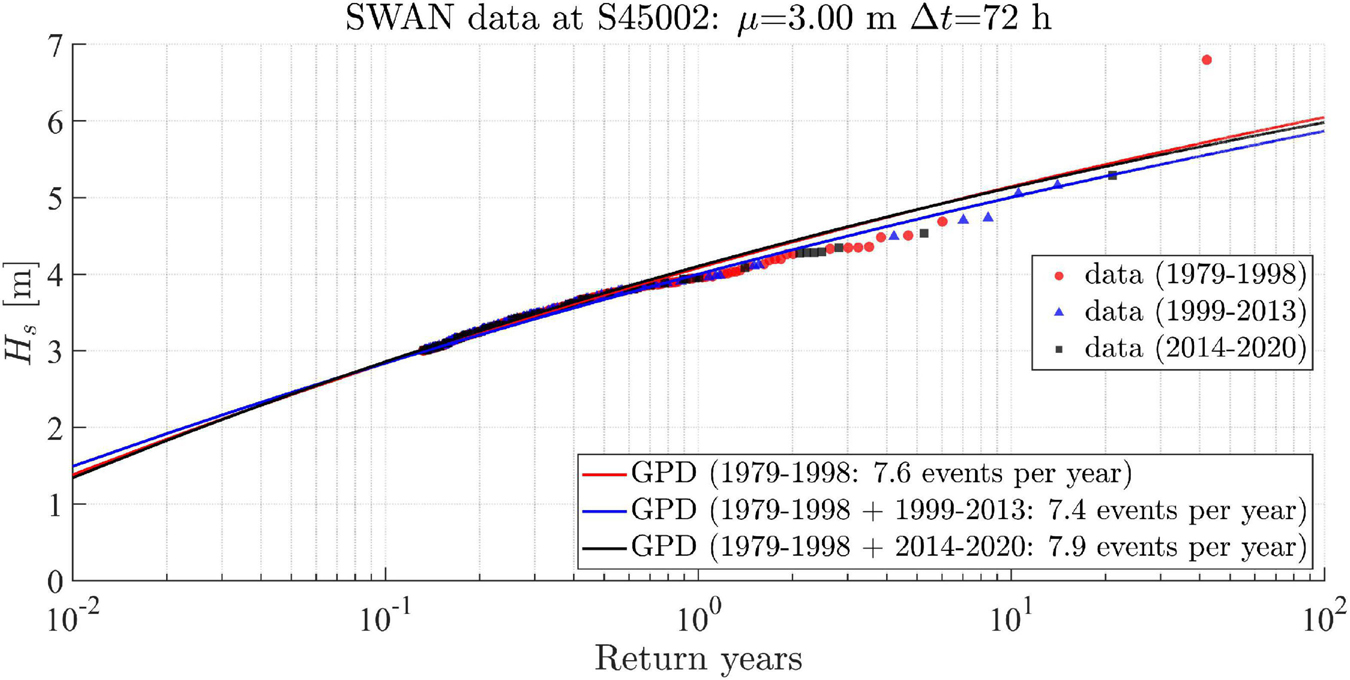
Figure 13. The return level of H_s calculated based on the Peaks Over Threshold (POT) method with the threshold μ=3 m and time interval Δt = 72 h. The three Generalized Pareto Distribution (GPD) based fitting lines are using the POT selected data in three periods. Period I: 1979–1998 (regime 1); period II: 1979–1998 plus 1999–2013 (regime 1 plus regime 2), and period III: 1979–1998 plus 2014–2020 (regime 1 plus regime 3).

Effects of Ice Reduction on Wave Climate

Ice cover can reduce wind stress and resulting wave energy. In addition, waves propagating in an ice field are reduced by a combination of scattering and dissipation. Due to the orientation of Lake Michigan, the northernmost part of the lake is characterized by a much higher ice cover percentage and longer ice duration, while the southern region has much less ice cover during the winter. Therefore, the trend and variability of ice cover and its impact on waves are much more significant in the northern lake. Recall that the northernmost part of the lake showed an increase in large (e.g., 99th percentile) wave heights in ice season (Figure 12A2) from the period of 1979–1998 (high water level) to the period of 1999–2013 (low water level), which is opposite to the downward trend observed in the most areas of the lake which had no or low ice cover. Such a difference was caused by the significant reduction in ice cover in favor of wave development that occurred in the northern lake during the period of 1999–2013 in comparison to the period of 1979–1998 (Figures 14A,B). It also explains why the northernmost part of the lake could show a statistically significant increase in wave height over the past 42 years, even with linear regress analysis. Lastly, results (Figures 12B2, 14C) suggest that the increased winter storms accompanied by the rising water level during the period of 2014–2020 were the dominant forcing for the increase in large waves, which overshadowed the negative influences of the moderate increase in ice cover in the northern lake on wave development.

FIGURE 14

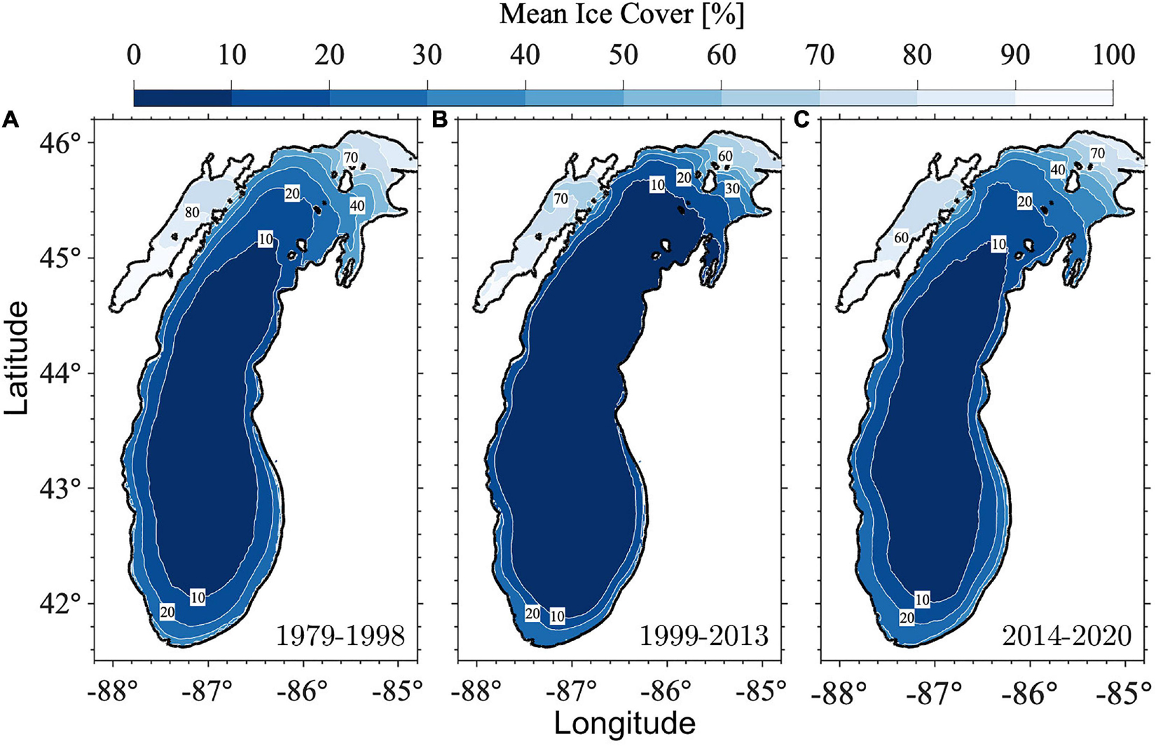
Figure 14. Mean ice cover from January to March during the three periods: (A) 1979–1998, (B) 1999–2013, and (C) 2014–2020.

Under projected regional warming, the observed reduction in ice coverage and ice duration in the Great Lakes are expected to continue into the future (Wang et al., 2012; Mason et al., 2016; USGCRP, 2017). To demonstrate the influence of changing ice conditions on the wave climate in Lake Michigan, we selected two representative historical years, which have low and high ice covers (2013, 2014) for case studies with both Type I and Type N analysis (Figure 15). The wind speeds averaged over the lake during the ice seasons were similar in the two years, with U₁₀ = 7.78 m/s in 2013 and U₁₀ 7.50 m/s in 2014. However, the averaged ice coverage in 2013 was only 11% compared to a much higher percentage of ice cover of 51% in the cold year of 2014. While the wind speed in 2014 ice season was only slightly lower than that in 2013 during the ice season (Figures 15A2,B2), the mean H_s in 2014 ice season was 0.2–0.8 m, which was significantly lower than that in 2013 during which the majority of the lake showed mean H_s between 0.8 and 1.2 m (Figures 15A3,B3, Type I statistics). In a warming scenario of no ice (the wave simulations in these 2 years were re-run under the condition without ice cover in the lake to demonstrate the impact of disappearing ice on the wave climate, Type N statistics), mean H_s would increase noticeably in the northernmost part of the lake, a region influenced the most by the ice cover, in the simulation of 2013. In the simulation of the cold year of 2014, a substantial increase by 50% in mean H_s would occur in the majority of the lake, with the most significant increase in the northern lake, where ice cover was the largest (Figures 15A4,B4). This again illustrated the influences of decreasing ice on wave development.

FIGURE 15

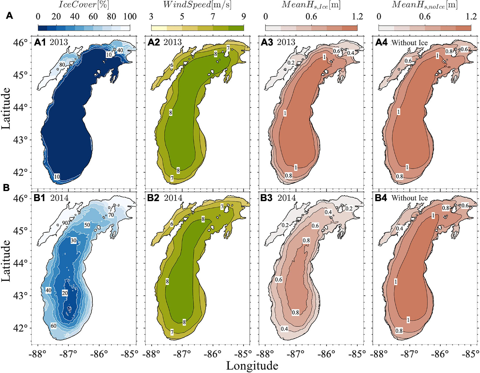
Figure 15. Mean ice cover, surface wind speed, significant wave height (H_s) from January to March with (Type I statistics) and without ice (Type N statistics) for two representative years under (A) small ice coverage in 2013 and (B) large ice coverage in 2014.

Conclusion

In this study, we investigated the wave climate associated with changing water level and ice cover in Lake Michigan. The main findings include: (1) long-term wave changes were poorly explained by a simple linear trend. Rather, we identified the several regime shifts of H_s that correspond to long-term lake water level changes. The coherent patterns of the waves and water levels were hypothesized to be due to the changes in the storms crossing the entire lake basin, which influenced the changes in waves (instantly through increased wind stress on the surface) and water levels (following, with a lag through precipitation and runoff). (2) The seasonal ice cover has a decisive impact on the wave climate. In our case studies, simulations with hypothetical no-ice conditions reveal that loss of ice cover can increase basin-wide mean wave height by 50% during the winter season. Under the projected climate, the regional air temperature is projected to increase by 3.3°C–6.0°C by the end of the century, depending on warming scenarios (Zhang et al., 2020). Correspondingly, the ice cover in the Great Lakes is expected to continue to decrease. Lake Michigan’s recently increasing wave heights and water levels, along with a warming climate and ice reduction, may yield increasing coastal damages such as accelerating coastal erosion and enhanced sediment transport.

Data Availability Statement

The original contributions presented in the study are included in the article/Supplementary Material, further inquiries can be directed to the corresponding author/s.

Author Contributions

PX, CH, GM, and GAM contributed to the conception and design of the study. CH conducted the model simulations. PX, CH, and LZ performed the data analysis and wrote the first draft of the manuscript. PX directed and supervised the project. All authors contributed to manuscript revision, read, and approved the submitted version.

Funding

This work was sponsored by Michigan Sea Grant College Program, Project Number Index R/SD-5, under award NA18OAR4170102 from National Sea Grant, NOAA, U.S. Department of Commerce, with funds from the State of Michigan. Hydrodynamic modeling was also supported, in part, by COMPASS-GLM, a multi-institutional project supported by the U.S. Department of Energy, Office of Science, Office of Biological and Environmental Research, Earth and Environmental Systems Modeling program. Financial assistance for this research was also provided, in part, by the Coastal Management Program, Water Resources Division, Michigan Department of Environment, Great Lakes, and Energy, under the National Coastal Zone Management Program, through a grant (NA18NOS4190162) from the National Oceanic and Atmospheric Administration, U.S. Department of Commerce.

Author Disclaimer

The statements, findings, conclusions, and recommendations provided are those of the authors and do not necessarily reflect the views of the Michigan Department of Environment, Great Lakes, Energy, or the National Oceanic and Atmospheric Administration.

Conflict of Interest

The authors declare that the research was conducted in the absence of any commercial or financial relationships that could be construed as a potential conflict of interest.

Publisher’s Note

All claims expressed in this article are solely those of the authors and do not necessarily represent those of their affiliated organizations, or those of the publisher, the editors and the reviewers. Any product that may be evaluated in this article, or claim that may be made by its manufacturer, is not guaranteed or endorsed by the publisher.

Acknowledgments

This is the contribution 83 of the Great Lakes Research Center at Michigan Technological University. The Michigan Tech high performance computing cluster, Superior, was used in obtaining the modeling results presented in this publication.

Supplementary Material

The Supplementary Material for this article can be found online at: https://www.frontiersin.org/articles/10.3389/fmars.2021.746916/full#supplementary-material

Footnotes

1. ^ https://www.weather.gov/lot/2011sep30
2. ^ https://www.weather.gov/lot/2014Oct31
3. ^ https://www.weather.gov/lot/2020March6_lakeshoreflooding
4. ^ https://rda.ucar.edu/datasets/ds093.1/
5. ^ https://rda.ucar.edu/datasets/ds094.1/
6. ^ https://www.glerl.noaa.gov/data/ice/#historical
7. ^ https://www.glerl.noaa.gov/data/ice/atlas/
8. ^ https://www.glerl.noaa.gov/data/dashboard/data/
9. ^ http://southhavensteelheaders.com/wp-content/uploads/2013/12/S2Yachts_TIDAS900-1.pdf
10. ^ https://www.seaviewsystems.com/products/data-buoy-instruments/svs-603-inertial-wave-sensor/
11. ^ http://swanmodel.sourceforge.net/

References

Aarnes, O. J., Breivik, Ø, and Reistad, M. (2012). Wave extremes in the northeast Atlantic. J. Climate 25, 1529–1543. doi: 10.1175/JCLI-D-11-00132.1

CrossRef Full Text | Google Scholar

Aboobacker, V. M., Vethamony, P., and Rashmi, R. (2011). “Shamal” swells in the Arabian sea and their influence along the west coast of India. Geophys. Res. Lett. 38, 1–7. doi: 10.1029/2010GL045736

CrossRef Full Text | Google Scholar

Anderson, J. D., Wu, C. H., and Schwab, D. J. (2015). Wave climatology in the apostle islands, Lake superior. J. Geophys. Res. Oceans 120, 4869–4890. doi: 10.1002/2014jc010278

CrossRef Full Text | Google Scholar

Assel, R., Cronk, K., and Norton, D. (2003). Recent trends in Laurentian great lakes ice cover. Clim. Change 57, 185–204. doi: 10.1023/a:1022140604052

CrossRef Full Text | Google Scholar

Bai, P., Wang, J., Chu, P., Hawley, N., Fujisaki-Manome, A., Kessler, J., et al. (2020). Modeling the ice-attenuated waves in the Great Lakes. Ocean Dyn. 70, 991–1003. doi: 10.1007/s10236-020-01379-z

CrossRef Full Text | Google Scholar

Bennetts, L. G., Peter, M. A., Squire, V. A., and Meylan, M. H. (2010). A three-dimensional model of wave attenuation in the marginal ice zone. J. Geophys. Res. 115:C12043. doi: 10.1029/2009JC005982

CrossRef Full Text | Google Scholar

Bennington, V., McKinley, G. A., Kimura, N., and Wu, C. H. (2010). General circulation of Lake superior: mean, variability, and trends from 1979 to 2006. J. Geophys. Res. Oceans 115:C12015.

Google Scholar

Benoit, M., Marcos, F., and Becq, F. (1997). Development of a third generation shallow-water wave model with unstructured spatial meshing. Coastal Eng. 1996, 465–478.

Google Scholar

Booij, N. R. R. C., Ris, R. C., and Holthuijsen, L. H. (1999). A third-generation wave model for coastal regions: 1. model description and validation. J. Geophys. Res. Oceans 104, 7649–7666. doi: 10.1029/98jc02622

CrossRef Full Text | Google Scholar

Bromirski, P. D., and Cayan, D. R. (2015). Wave power variability and trends across the North Atlantic influenced by decadal climate patterns. J. Geophys. Res. Oceans 120, 3419–3443. doi: 10.1002/2014jc010440

CrossRef Full Text | Google Scholar

Caires, S., and Sterl, A. (2005). A new nonparametric method to correct model data: application to significant wave height from the ERA-40 re-analysis. J. Atmospheric Oceanic Technol. 22, 443–459. doi: 10.1175/jtech1707.1

CrossRef Full Text | Google Scholar

Camus, P., Menéndez, M., Méndez, F. J., Izaguirre, C., Espejo, A., Cánovas, V., et al. (2014). A weather-type statistical downscaling framework for ocean wave climate. J. Geophys. Res. Oceans 119, 7389–7405. doi: 10.1002/2014jc010141

CrossRef Full Text | Google Scholar

Carter, D. J. T. (1982). Prediction of wave height and period for a constant wind velocity using the JONSWAP results. Ocean Eng. 9, 17–33. doi: 10.1016/0029-8018(82)90042-7

CrossRef Full Text | Google Scholar

Cheng, T. K., Hill, D. F., Beamer, J., and García-Medina, G. (2015). Climate change impacts on wave and surge processes in a Pacific Northwest (USA) estuary. J. Geophys. Res. Oceans 120, 182–200. doi: 10.1002/2014jc010268

CrossRef Full Text | Google Scholar

Coles, S. (2001). An Introduction to Statistical Modeling of Extreme Values. London: Springer.

Google Scholar

Deacu, D., Klyszejko, E., Spence, C., and Blanken, P. (2012). Predicting the net basin supply to the great lakes with a hydrometeorological model. Bull. Am. Met. Soc. 13, 1739–1759. doi: 10.1175/JHM-D-11-0151

CrossRef Full Text | Google Scholar

Dietrich, J. C., Westerink, J. J., Kennedy, A. B., Smith, J. M., Jensen, R. E., Zijlema, M., et al. (2011). Hurricane Gustav (2008) waves and storm surge: hindcast, synoptic analysis, and validation in Southern Louisiana. Monthly Weather Rev. 139, 2488–2522.

Google Scholar

Doble, M. J., De Carolis, G., Meylan, M. H., Bidlot, J., and Wadhams, P. (2015). Relating wave attenuation to pancake ice thickness, using field measurements and model results. Geophys. Res. Lett. 42, 4473–4481. doi: 10.1002/2015GL063628

CrossRef Full Text | Google Scholar

Donelan, M. A., Hamilton, J., and Hui, W. (1985). Directional spectra of wind-generated ocean waves. Philos. Trans. R. Soc. London Ser. A Mathe. Phys. Sci. 315, 509–562. doi: 10.1098/rsta.1985.0054

CrossRef Full Text | Google Scholar

Gronewold, A. D., and Rood, R. B. (2019). Recent water level changes across Earth’s largest lake system and implications for future variability. J. Great Lakes Res. 45, 1–3.

Google Scholar

Group, W. A. M. D. I. (1988). The WAM modela third generation ocean wave prediction model. J. Phys. Oceanogr. 18, 1775–1810.

Google Scholar

Huang, C., Anderson, E. J., Liu, Y., Ma, G., Mann, G., and Xue, P. (2021). Evaluating essential processes and forecast requirements for meteotsunami-induced coastal flooding. Nat. Hazards. doi: 10.1007/s11069-021-05007-x

CrossRef Full Text | Google Scholar

Huang, Y., Weisberg, R. H., Zheng, L., and Zijlema, M. (2013). Gulf of Mexico hurricane wave simulations using SWAN: bulk formula-based drag coefficient sensitivity for Hurricane Ike. J. Geophys. Res. Oceans 118, 3916–3938.

Google Scholar

Hubertz, J. M., Driver, D. B., and Reinhard, R. D. (1991). Wind waves on the great Lakes: a 32 year hindcast. J. Coast. Res. 7, 945–967.

Google Scholar

Jabbari, A., Ackerman, J. D., Boegman, L., and Zhao, Y. (2021). Increases in great Lake winds and extreme events facilitate interbasin coupling and reduce water quality in Lake Erie. Sci. Rep. 11:5733. doi: 10.1038/s41598-021-84961-9

PubMed Abstract | CrossRef Full Text | Google Scholar

Jensen, R. E., Cialone, M. A., Chapman, R. S., Ebersole, B. A., Anderson, M., and Thomas, L. (2012). Lake Michigan Storm: Wave and Water Level Modeling (No. ERDC/CHL-TR-12-26). Vicksburg, MS: Engineer research and development center vicksburg ms coastal and hydraulics lab.

Google Scholar

Kohout, A. L., Meylan, M. H., and Plew, D. R. (2017). Wave attenuation in a marginal ice zone due to the bottom roughness of ice floes. Ann. Glaciol. 52, 118–122. doi: 10.3189/172756411795931525

CrossRef Full Text | Google Scholar

Lin, W., Sanford, L. P., and Suttles, S. E. (2002). Wave measurement and modeling in Chesapeake Bay. Continental Shelf Res. 22, 2673–2686. doi: 10.1016/S0278-4343(02)00120-6

CrossRef Full Text | Google Scholar

Lin, Y. T., and Wu, C. H. (2014). A field study of nearshore environmental changes in response to newly-built coastal structures in Lake Michigan. J. Great Lakes Res. 40, 102–114.

Google Scholar

Mao, M., Van Der Westhuysen, A. J., Xia, M., Schwab, D. J., and Chawla, A. (2016). Modeling wind waves from deep to shallow waters in Lake Michigan using unstructured SWAN. J. Geophys. Res. Oceans 121, 3836–3865. doi: 10.1002/2015jc011340

CrossRef Full Text | Google Scholar

Mason, L. A., Riseng, C. M., Gronewold, A. D., Rutherford, E. S., Wang, J., Clites, A., et al. (2016). Fine-scale spatial variation in ice cover and surface temperature trends across the surface of the Laurentian Great Lakes. Clim. Change 138, 71–83. doi: 10.1007/s10584-016-1721-2

CrossRef Full Text | Google Scholar

Meadows, G. A., Meadows, L. A., Wood, W. L., Hubertz, J. M., and Perlin, M. (1997). The relationship between Great Lakes water levels, wave energies, and shoreline damage. Bull. Am. Meteorol. Soc. 78, 675–684. doi: 10.1175/1520-0477(1997)078<0675:trbglw>2.0.co;2

CrossRef Full Text | Google Scholar

Méndez, F. J., Menéndez, M., Luceño, A., and Losada, I. J. (2006). Estimation of the long-term variability of extreme significant wave height using a time-dependent peak over threshold (POT) model. J. Geophys. Res. Oceans 111, 1–13. doi: 10.1029/2005JC003344

CrossRef Full Text | Google Scholar

Niroomandi, A., Ma, G., Ye, X., Lou, S., and Xue, P. (2018). Extreme value analysis of wave climate in Chesapeake Bay. Ocean Eng. 159, 22–36. doi: 10.1016/j.oceaneng.2018.03.094

CrossRef Full Text | Google Scholar

Olsen, N. R. (2019). Long Term Trends in Lake Michigan Wave Climate. Master Thesis, Purdue University Graduate School, West Lafayette, IN. doi: 10.25394/PGS.7999142.v1

CrossRef Full Text | Google Scholar

Panchang, V., Jeong, C. K., and Demirbilek, Z. (2013). Analyses of extreme wave heights in the Gulf of Mexico for offshore engineering applications. J. Off. Mech. Arctic Eng. 135:031104.

Google Scholar

Pore, N. A. (1979). Automated wave forecasting for the great lakes. Monthly Weather Rev. 107, 1275–1286. doi: 10.1175/1520-04931979107<1275:AWFFTG<2.0.CO;2

CrossRef Full Text | Google Scholar

Resio, D., and Perrie, W. (1989). Implications of an f^(-4) equilibrium range for wind-generated waves. J. Phys. Oceanogr. 19, 193–204.

Google Scholar

Rogers, W. E., Hwang, P. A., and Wang, D. W. (2003). Investigation of wave growth and decay in the SWAN model: three regional-scale applications. J. Phys. Oceanogr. 33, 366–389. doi: 10.1175/1520-0485(2003)033<0366:iowgad>2.0.co;2

CrossRef Full Text | Google Scholar

Rogers, W. E., Kaihatu, J. M., Hsu, L., Jensen, R. E., Dykes, J. D., and Holland, K. T. (2007). Forecasting and hindcasting waves with the SWAN model in the Southern California Bight. Coast. Eng. 54, 1–15. doi: 10.1016/j.coastaleng.2006.06.011

CrossRef Full Text | Google Scholar

Sabique, L., Annapurnaiah, K., Balakrishnan Nair, T. M., and Srinivas, K. (2012). Contribution of southern indian ocean swells on the wave heights in the northern indian ocean—a modeling study. Ocean Eng. 43, 113–120. doi: 10.1016/j.oceaneng.2011.12.024

CrossRef Full Text | Google Scholar

Saha, S., Moorthi, S., Pan, H. L., Wu, X., Wang, J., Nadiga, S., et al. (2010). NCEP Climate Forecast System Reanalysis (CFSR) 6-Hourly Products, January 1979 to December 2010. Boulder, CO: Research Data Archive at the National Center for Atmospheric Research, Computational and Information Systems Laboratory.

Google Scholar

Saha, S., Moorthi, S., Wu, X., Wang, J., Nadiga, S., Tripp, P., et al. (2011). NCEP Climate Forecast System Version 2 (CFSv2) 6-Hourly Products. Boulder, CO: Research Data Archive at the National Center for Atmospheric Research, Computational and Information Systems Laboratory.

Google Scholar

Schwab, D. J., Eadie, B. J., Assel, R. A., and Roebber, P. J. (2006). Climatology of large sediment resuspension events in southern Lake Michigan. J. Great Lakes Res. 32, 50–62. doi: 10.3394/0380-1330(2006)32[50:colsre]2.0.co;2

CrossRef Full Text | Google Scholar

Sutherland, G., and Rabault, J. (2016). Observations of wave dispersion and attenuation in landfast ice. J. Geophys. Res. Oceans 121, 1984–1997. doi: 10.1002/2015JC011446

CrossRef Full Text | Google Scholar

Swenson, M. J., Wu, C. H., Edil, T. B., and Mickelson, D. M. (2006). Bluff recession rates and wave impact along the Wisconsin coast of Lake Superior. J. Great Lakes Res. 32, 512–530. doi: 10.3394/0380-1330(2006)32[512:brrawi]2.0.co;2

CrossRef Full Text | Google Scholar

Thomasen, S., Gilbert, J., and Chow-Fraser, P. (2013). Wave exposure and hydrologic connectivity create diversity in habitat and zooplankton assemblages at nearshore Long Point Bay, Lake Erie. J. Great Lakes Res. 39, 56–65. doi: 10.1016/j.jglr.2012.12.014

CrossRef Full Text | Google Scholar

Thyng, K., Greene, C., Hetland, R., Zimmerle, H., and DiMarco, S. (2016). True colors of oceanography: guidelines for effective and accurate Colormap selection. Oceanography 29, 9–13. doi: 10.5670/oceanog.2016.66

CrossRef Full Text | Google Scholar

Tolman, H. L. (1991). A third-generation model for wind waves on slowly varying, unsteady, and inhomogeneous depths and currents. J. Phys. Oceanogr. 21, 782–797. doi: 10.1175/1520-0485(1991)021<0782:atgmfw>2.0.co;2

CrossRef Full Text | Google Scholar

Trewin, B. C. (2007). The Role of Climatological Normals in a Changing Climate. Switzerland: World Meteorological Organization.

Google Scholar

Tuomi, L., Kahma, K. K., and Pettersson, H. (2011). Wave hindcast statistics in the seasonally ice-covered Baltic Sea. Boreal Environ. Res. 16, 451–472.

Google Scholar

Tuomi, L., Kanarik, H., Björkqvist, J. V., Marjamaa, R., Vainio, J., Hordoir, R., et al. (2019). Impact of ice data quality and treatment on wave hindcast statistics in seasonally ice-covered seas. Front. Earth Sci. 7:166. doi: 10.3389/feart.2019.00166

CrossRef Full Text | Google Scholar

USGCRP (2017). Climate Science Special Report: Fourth National Climate Assessment, Vol. I eds D. J. Wuebbles, D. W. Fahey, K. A. Hibbard, D. J. Dokken, B. C. Stewart, and T. K. Maycock Washington, DC: U.S. Global Change Research Program), 470. doi: 10.7930/J0J964J6

CrossRef Full Text | Google Scholar

Velioglu Sogut, D., Farhadzadeh, A., and Jensen, R. E. (2018). Characterizing the great lakes marine renewable energy resources: Lake Michigan surge and wave characteristics. Energy 150, 781–796. doi: 10.1016/j.energy.2018.03.031

CrossRef Full Text | Google Scholar

Vieira, F., Cavalcante, G., and Campos, E. (2020). Analysis of wave climate and trends in a semi-enclosed basin (Persian Gulf) using a validated SWAN model. Ocean Eng. 196:106821. doi: 10.1016/j.oceaneng.2019.106821

CrossRef Full Text | Google Scholar

Voermans, J. J., Babanin, A. V., Thomson, J., Smith, M. M., and Shen, H. H. (2019). Wave attenuation by sea ice turbulence. Geophys. Res. Lett. 46, 6796–6803. doi: 10.1029/2019GL082945

CrossRef Full Text | Google Scholar

Wandres, M., Aucan, J., Espejo, A., Jackson, N., De Ramon, N., Yeurt, A., et al. (2020). Distant-source swells cause coastal inundation on fiji’s coral coast. Front. Mari. Sci. 7:1–10. doi: 10.3389/fmars.2020.00546

CrossRef Full Text | Google Scholar

Wang, J., Bai, X., Hu, H., Clites, A., Colton, M., and Lofgren, B. (2012). Temporal and spatial variability of Great Lakes ice cover, 1973–2010. J. Clim. 25, 1318–1329. doi: 10.1175/2011jcli4066.1

CrossRef Full Text | Google Scholar

Wang, X. L., Feng, Y., and Swail, V. R. (2015). Climate change signal and uncertainty in CMIP5-based projections of global ocean surface wave heights. J. Geophys. Res. Oceans 120, 3859–3871. doi: 10.1002/2015jc010699

CrossRef Full Text | Google Scholar

Xie, D., Zou, Q., and Cannon, J. W. (2016). Application of SWAN+ADCIRC to tide-surge and wave simulation in Gulf of Maine during Patriot’s Day storm. Water Sci. Eng. 9, 33–41. doi: 10.1016/j.wse.2016.02.003

CrossRef Full Text | Google Scholar

Xie, D., Zou, Q.-P., Mignone, A., and MacRae, J. D. (2019). Coastal flooding from wave overtopping and sea level rise adaptation in the northeastern USA. Coast. Eng. 150, 39–58. doi: 10.1016/j.coastaleng.2019.02.001

CrossRef Full Text | Google Scholar

Xue, P., Schwab, D. J., and Hu, S. (2015). An investigation of the thermal response to meteorological forcing in a hydrodynamic model of Lake Superior. J. Geophys. Res. Oceans 120, 5233–5253. doi: 10.1002/2015jc010740

CrossRef Full Text | Google Scholar

Yiew, L. J., Parra, S. M., Wang, D., Sree, D. K. K., Babanin, A. V., and Law, A. W.-K. (2019). Wave attenuation and dispersion due to floating ice covers. Appl. Ocean Res. 87, 256–263. doi: 10.1016/j.apor.2019.04.006

CrossRef Full Text | Google Scholar

Zhang, L., Zhao, Y., Hein-Griggs, D., Janes, T., Tucker, S., and Ciborowski, J. J. (2020). Climate change projections of temperature and precipitation for the great lakes basin using the PRECIS regional climate model. J. Great Lakes Res. 46, 255–266. doi: 10.1016/j.jglr.2020.01.013

CrossRef Full Text | Google Scholar