Internal Wave Dynamics Over Isolated Seamount and Its Influence on Coral Larvae Dispersion

The internal wave dynamics over Rosemary Bank Seamount (RBS), North Atlantic, were investigated using the Massachusetts Institute of Technology general circulation model. The model was forced by M2-tidal body force. The model results are validated against the in-situ data collected during the 136th cruise of the RRS “James Cook” in June 2016. The observations and the modeling experiments have shown two-wave processes developed independently in the subsurface and bottom layers. Being super-critical topography for the semi-diurnal internal tides, RBS does not reveal any evidence of tidal beams. It was found that below 800-m depth, the tidal flow generates bottom trapped sub-inertial internal waves propagated around RBS. The tidal flow interacting with a cluster of volcanic origin tall bottom cones generates short-scale internal waves located in 100 m thick seasonal pycnocline. A weakly stratified layer separates the internal waves generated in two waveguides. Parameters of short-scale sub-surface internal waves are sensitive to the season stratification. It is unlikely they can be observed in the winter season from November to March when seasonal pycnocline is not formed. The deep-water coral larvae dispersion is mainly controlled by bottom trapped tidally generated internal waves in the winter season. A Lagrangian-type passive particle tracking model is used to reproduce the transport of generic deep-sea water invertebrate species.

1. Introduction

The life of deep-water corals, their nutrition, sustainability, and survival in the conditions of climate change is in the focus of many studies (e.g., de Mol et al., 2002; van Weering et al., 2003; Roberts et al., 2006). In a deep water environment below 500 m the ocean dynamics are usually not sensitive to the processes developing in the surface layer, e.g., wind-driven circulation or surface currents. Still, they can be affected by internal waves and tidally induced residual water transport (White and Dorschel, 2010). As it was reported by Henry et al. (2014) and Davison et al. (2019), the primary source for food and oxygen supply to these deep-water communities usually has a tidal origin.

The mechanism of water mixing and deep-water coral feeding is related to tidal activity. Tidal currents streamlining bumpy bottom topography provide vertical fluxes of nutrients required for the initial biological production. They generate internal waves in the vertically stratified ocean and produce water mixing, which facilitates the dispersion of chemicals (Henry et al., 2014). The importance of internal wave mixing and internal tides for the sustainability of cold-water coral communities is well-recognized. It is underpinned by many observations and theoretical studies, specifically conducted for underwater banks. For instance, Mohn and White (2010) in their modeling paper has shown how the tidal activity over the oceanic bank can affect the sea environment, specifically the deep-water corals' communities. The principal conclusion formulated in this paper is that the tidal motions in the areas of underwater seamounts have not just local but far-field effects on the deep-water coral dispersion. The investigation of the tidal actions is the topic of the present paper as well, although we consider not an idealized symmetrical oceanic bank but the natural area in the North Atlantic, which includes Rosemary Bank Seamount (RBS).

One of the recent publications based on observations, Soetaert et al. (2016), sheds light on the way how the organic matter is supplied to the deep-water corals. This particular study concerns the Rockall Bank area, which is close to RBS considered in the present paper. In general, all local studies conducted in the North Atlantic and referred here help understand the link between deep-water coral communities, their nutrition, and surface water productivity. The latter is a generic problem for many areas of the Global Ocean. The authors appreciate the significant role of internal tides and internal wave mixing in organic matter supply to the deep-water corals.

Significant progress in understanding the cold-water coral occurrence and the role of tidally induced water activity in the North Atlantic was reported by van Harren et al. (2014). The study of Mohn et al. (2014) based on high-resolution numerical modeling using the ROMS model and highlighted many exciting effects introduced by tides generated over underwater banks, specifically the role of trapped internal waves, radiated internals, and internal jumps. The results reported in the present paper are based on a similar approach of a combination of the observational data set and high-resolution modeling applied to a different area, Rosemary Bank Seamount. Our findings are in line with the conclusions of the paper by Cyr et al. (2016) who acknowledged a strong influence of the baroclinic tidal hydrodynamics on the sustainability of the coral communities in the Rockall Bank area.

In the present paper, we make another attempt to look at the deep-water coral life based on the available in-situ collected data and the results of high-resolution modeling. The North Atlantic area considered here is Rosemary Bank Seamount, close to the Rockall Bank reported in the papers mentioned above. The observational data collected during the 136th cruise of the RRS “James Cook” (hereafter JC136) to the North-East Atlantic in May–June 2016. The coral samples were collected from the flanks of Anton Dohrn Seamount, Rockall Bank, George Bligh Seamount, Rosemary Bank Seamount, and slopes of the Wyville Thomson Ridge, Figure 1A, using the remotely operating vehicle (ROV) ISIS 5000.

FIGURE 1

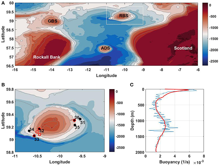
Figure 1. (A) Overview map showing the main topographic features in the NE Atlantic: GBS, George Bligh Seamount; RBS, Rosemary Bank Seamount; ADS, Anton Dohrn Seamount. Zoom of the dashed rectangle is shown in panel (B) with the plan view of the JC136 CTD stations at Rosemary Bank Seamount (filled black circles) and ROV missions (red circles). (C) Buoyancy frequency averaged over the data collected at the CTD stations.

The biological campaign was accompanied by oceanographic measurements that included a series of CTD (Conductivity, Temperature, Depth) stations and the deployment of two moorings in the area of Anton Dohrn Seamount. The analysis of the generation of internal waves by tides in areas of Anton Dohrn Seamount and the Wyville Thomson Ridge was reported in Vlasenko et al. (2018), Stashchuk et al. (2018), and Vlasenko and Stashchuk (2018).

The focus of the present paper is on Rosemary Bank Seamount. The tidal activity in the area is studied based on in-situ data and numerical modeling considering the semidiurnal M₂-tide (Egbert and Erofeeva, 2002) as the predominant tidal constituent (the discharge of the M2 tidal constituent is seven times greater than any other tidal harmonics). Another objective of the modeling efforts was defining the role of tidally generated dynamical processes, developing in the area around RBS in the dispersion of larvae released by deep water corals.

The paper is organized as follows. The observational data set that motivated the study and helped formulate the hypothesis is discussed in section 2. The model parameters and their setting are described in section 3. Internal wave generation over RBS with the detailed discussion of two wave-guide dynamics is the objective of section 4. In section 5, the analysis of model-predicted larvae tracks forced by tidal currents is presented. The paper finishes with a discussion and main conclusions.

2. Observations and Hypothesis

The observational data set for RBS includes temperature, salinity, and density profiles recorded at six CTD stations, Figure 1B. The buoyancy frequency profile, N²(z) = −g/ρ(∂ρ/∂z) (g is the acceleration due to gravity, and ρ is the water density), Figure 1C, is based on the density data averaged at all stations. It reveals the presence of two pycnoclines: (i) a very sharp seasonal pycnocline in the surface layer with its maximum at a depth of 50 m, and (ii) a weaker main one at the 1,200-m depth, that stretched from 800 to 1500 m.

A Lowered Acoustic Doppler Current Profiler (LADCP) was mounted on a CTD frame for recording instantaneous horizontal velocities. The LADCP data were processed using the method described by Visbeck (2002). Figure 2 shows that collected velocity profiles reveal an intensification of bottom currents below 800 m at all deep-water stations (except shallow water station 32). It was assumed that such an intensification of bottom currents could be caused by internal waves generated by tides at RBS: (i) tidal beam by internal waves and/or (ii) bottom trapped sub-inertial internal waves.

FIGURE 2

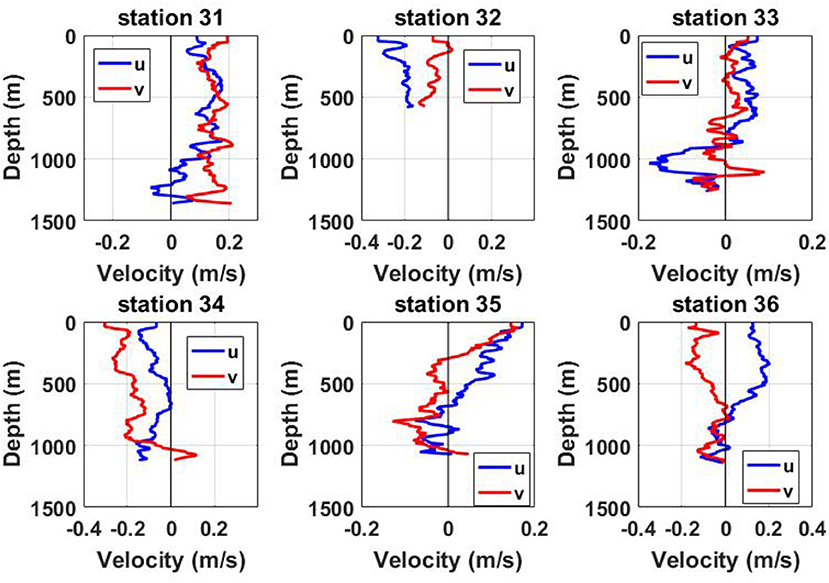
Figure 2. Instant vertical profiles of eastward (u) and northward (v) velocities recorded by LADCP at CTD stations.

The condition for tidal beam generation is controlled by a relative steepness of the bottom topography γ:

$\begin{array}{l}\gamma =\frac{|\nabla \left[H(x,y)\right]|}{\alpha \left[H(x,y)\right]},\end{array}$

which is a ratio of the topography steepness |∇[H(x, y)]| at a point (x, y) (x and y are horizontal coordinates and H is the water depth) to the inclination of tidal beam α at this point:

$\begin{array}{ll}\alpha \left[H(x,y)\right]=\frac{{\omega }^2-f^2}{N^2\left[H(x,y)\right]-{\omega }^2}.& (1)\end{array}$

Here f is the Coriolis parameter, ω is the tidal frequency, and N is the buoyancy frequency at the bottom point H(x, y). The internal tidal velocity forms the tidal beams in areas where γ ~ 1 (critical case) or γ > 1 (supercritical conditions). The beams present relatively narrow stripes with a considerable concentration of baroclinic energy (Bell, 1975).

Another possibility of bottom current intensification in the considered area could be sub-inertial bottom trapped internal waves. The theory of this type of motion was developed and discussed in many papers (e.g., Wang and Mooers, 1976; LeBlond and Mysak, 1978). Observational evidence and theoretical interpretation of such internal wave dynamics were reported recently by the authors for the Malin Shelf (Stashchuk and Vlasenko, 2017). The focus of the present paper is on the RBS area. The analysis is based on in-situ collected data set and model experiments that show a bottom current intensification below 1,000 m depth.

Our analysis relies on the results of previous studies that considered similar problems of bottom trapped internal waves generated by tides. The tidal flow interacting with seamounts generates internal waves radiated from the bottom obstruction in all directions. Linear theory predicts that internal waves are radiated from the topography when ω > f but are trapped in the place of the generation when ω < f. Note that as Huthnance (1978) and Dale et al. (2001) found, the generation mechanism is not so sensitive to the Earth rotation as the linear theory predicts in the case when the tidal frequency ω is close to the Coriolis parameter (inertial frequency f). There is no sharp jump from near-inertial to sub-inertial regimes of internal tides generation. As was reported by Huthnance (1978) and Dale et al. (2001), the generated over two-dimensional slopes internal waves at the latitude close to the critical are “nearly trapped by topography.” They considered a slightly super-inertial (ω/f=0.9), slightly sub-inertial (ω/f=1.1), and strongly sub-inertial (ω/f=1.5) cases. It was found that freely radiated internal waves can exist only when ω/f > 1, although the bottom trapped waves propagated along the slope are allowed in all considered bands.

Note that RBS is located at 59^oN latitude. According to Dale et al. (2001) classification, the RBS area falls into a slightly sub-inertial frequency band with the tidal frequency ω/f=1.1. As predicted, the sub-inertial bottom trapped internal waves are quite possible there. Thus, the strong, deep-water currents recorded in the JC136th cruise can be associated with the generation of internal tidal beams (as it was in the case of Anton Dohrn Seamount, Vlasenko et al., 2018) or/and bottom trapped sub-inertial internal waves. Clarification of which of these mechanisms caused the observed bottom currents was the motivation of the present study.

3. The Model

Modeling the tidal motions in the RBS area was conducted using the Massachusetts Institute of Technology general circulation model (MITgcm) (Marshall et al., 1997) in its fully nonlinear and nonhydrostatic three-dimensional version. We used the Cartesian coordinate system with x-axis directed to the east and y-axis directed to the north and vertical z axis (z = 0 at the free surface). The topography presented in Figure 1B was approximated by 815 × 698 model grid with a horizontal resolution of 115.75 m in both zonal and meridional directions. Extra 128 grid steps were added to the northern, southern, western, and eastern boundaries, transforming it into a 1,071 × 954 grid. In these lateral areas, the grid resolution gradually changes from a 115.75 m spatial step in its central part to 2 × 10⁸ m at the boundary. Such a telescopic increase of the horizontal steps toward the periphery eliminated the reflection of the waves from the model boundaries for at least 12 tidal cycles. In the vertical direction, the water depth was restricted by a 2,000-m isobath. The vertical model resolution was Δz = 10 m.

The M2-tide was activated in the model using a body force introduced into the right-hand side of the momentum balance equations. The details of the tidal body force method and its justification are described in Vlasenko and Stashchuk (2021). The tides were set in the model using the data from the inverse tidal model TPXO 8.1 (Egbert and Erofeeva, 2002).

The vertical turbulent closure for the coefficients of viscosity A^v and diffusivity K^v was provided by the Richardson number dependent parameterization, Pacanowski and Philander (1981), (PP81 scheme):

$\begin{array}{r}{A}^v=\frac{A_0^v}{{(1+a\text{Ri})}^n}+A_b^v,\\ K^v=\frac{A^v}{(1+a\text{Ri})}+K_b^v.& (2)\end{array}$

Here Ri is the Richardson number, $\mathrm{\text{Ri}}=N^2(z)/(u_z^2+v_z^2)$, and, u and v are the zonal and meridional components of horizontal velocity; $A_b^v$=10⁻⁵ m² s⁻¹ and $K_b^v$=10⁻⁵ m² s⁻¹ are the background viscosity/diffusion parameters, respectively, $A_0^v$=1.5·10⁻² m² s⁻¹, a=5 and n=1 are the adjustable parameters. The PP81 scheme increases the coefficients A^v and K^v in the areas with the small Richardson numbers, which dumps shear instabilities and stabilizes inverse water stratification produced by breaking internal waves.

All model runs were conducted with constant horizontal viscosity A^h and diffusivity K^h coefficients at the level of 0.5 m² s⁻¹. Technically, the model produced 1-h outputs for velocities and thermohaline data. In addition to that, the model delivered 1-min outputs of the vertical temperature and velocities sampling at the position of six CTD-LADCP stations, Figure 1B.

The great performance of the MITgcm on replication of internal tides was already checked and reported in many papers (e.g., Vlasenko et al., 2013, 2014, 2016, 2018; Stashchuk et al., 2014, 2017, 2018; Stashchuk and Vlasenko, 2017). These publications have shown the consistency of the observational data sets and the modeling outputs. On a quantitative level, the correlation coefficient between the MITgcm model predictions and observations was calculated and reported in Vlasenko et al. (2014). It was found that the correlation coefficient r between theoretical and observational velocity time series was at the level of 0.7, which is great for the model predictions (for the details, see the Supplementary Material).

Another quantitative measure of the consistency of the modeling results with the observational data sets is the index of agreement d introduced by Willmott (1981, 1982) (Supplementary Material). As we found in our modeling experiments, the extent to which the model output is error-free is quite good. In general, the index of agreement d can vary from 0 (absolute disagreement) to 1 (perfect coincidence). The value of d estimated here was 0.7, which shows a good agreement between the observations and the model results.

4. Tidal Wave Dynamics

The internal wave dynamics in underwater seamount areas are sensitive to the intensity of tidal flow, water stratification, background mixing, and configuration of the bottom topography. The latter controls the spatial variability and spectral properties of the generated waves.

The summit of RBS above 800 m isobath (thick black line in Figure 3A) is relatively flat. Beneath this depth, the bottom is supercritical in terms of internal tide generation, i.e., the parameter γ > 1 (white color in Figure 3A). In this case, one of the expected scenarios would be a generation of internal wave beams at the RBS flanks, which radiate the tidal energy to the surface, Vlasenko et al. (2016, 2018). If this is the case, the beams should dominate in the model-predicted baroclinic velocity output. They can be evident after removing the barotropic tidal signal. However, closer inspection of the amplitudes of horizontal velocities along the transects crossing the positions of stations 31 and 33, Figure 3, does not show any sign of strong tidal beams over the RBS periphery. The model-predicted velocity amplitudes reveal two areas of intense baroclinic tidal signal—in the surface 100 m layer, and below 800-m of depth. As modeling results show, these two wave structures, i.e., (i) surface located internal waves and (ii) bottom trapped waves, develop independently without any apparent influence on each other. Such a structure of wave fields developed independently can be explained in terms of two waveguides dynamics. Figure 1C shows the presence of two pycnoclines, a thin surface 100 m stratified layer (seasonal pycnocline), and thick, deep stratified layer located between 800 and 1,500 m depth. Weakly stratified intermediate water separates two stratified layers, surface seasonal pycnocline and deep main pycnocline. This type of stratification can create conditions for two waveguide internal wave dynamics.

FIGURE 3

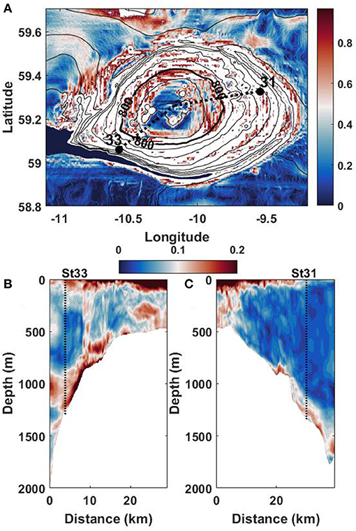
Figure 3. (A) Distribution of parameter γ overlaid with the RBS topography. Areas with γ > 1 are shown in white. Black dotted lines show cross-sections started at positions of CTD stations 31 and 33. (B,C) The model predicted amplitude of horizontal velocity in cross-sections shown in (A).

The model-predicted time series of eastward and northward velocities for stations 31 and 33 were considered to check the idea of two independent waveguides. Figures 4A,B present these data for station 31, and Figures 4C,D for station 33. The model output supports the hypothesis of two internal waveguides. They are separated by the layer with a strong barotropic tidal signal which does not reveal any baroclinic activity (constant velocity between 100 and 1,100 m depth). The velocity structure in this layer is nearly the same through the whole water column with sine-type periodicity in time. Note that thin surface 100- and 250-m thick bottom layers demonstrate quite a different wave activity. Horizontal motions in these layers are not in phase with the principal part of the water column (this is obvious in all velocity series of Figure 4).

FIGURE 4

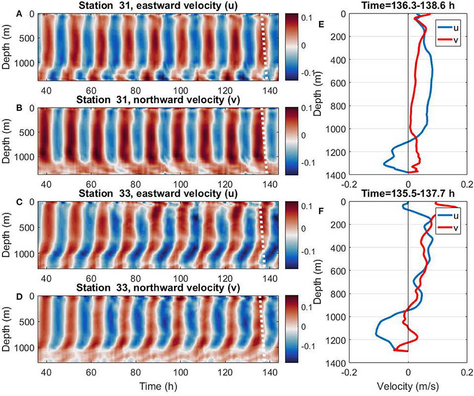
Figure 4. The model predicted time series of the eastward (A,C), and northward (B,D) velocities for stations 31 and 33. (E) Vertical profiles of the velocity components for station 31 after 136.3 h of the model time (shown by the white dashed line in A,B). (F) Vertical profiles of the velocity components for station 33 after 135.5 h of the model time (shown by the white dashed line in C,D).

Similar sampling was arranged in numerical experiments to compare the model predictions with the observational LADCP time series. Figure 4F (station 31) and Figure 4D (station 33) present instant vertical profiles of horizontal velocities at one particular moment of time depicted in Figures 4A–D by white dashed lines. These profiles show the consistency of the observational records for stations 31 and 33, with the model output, Figure 2. The velocity profiles at all CTD-LADCP stations, Figure 2, can be treated in terms of the formulated hypothesis of two internal waveguides separated by a thick intermediate layer. (Some extra Figures for four other CTD stations are shown in the Supplementary Material Document.)

The principal conclusion from the comparative analysis of the model outputs and the in-situ collected data can be formulated as follows: the intensification of the bottom located horizontal currents below 800 m depth is not associated with the tidal beams but has a different origin. One of the possible mechanisms is bottom trapped internal waves which are discussed below.

4.1. Bottom Trapped Sub-inertial Internal Waves

The intensification of bottom currents over RBS, Figures 2, 3, could be generated by bottom trapped internal waves. The theoretical background of such types of motions was provided by Huthnance (1978) who developed an analytical solution for trapped internal waves. This study was completed later by Dale et al. (2001) who provided some numerical evidence explaining the properties of the bottom-trapped internal waves at the transition from sub-inertial to super-inertial regimes of generation. Here we present a brief extract from the theory which is relevant to the RBS area.

Consider a periodical bottom trapped internal wave exp[i(ky+ωt)] propagated in a stratified fluid with the buoyancy frequency N(z) along a two-dimensional topography H(x). Here x and y are referred to as horizontal 0x and 0y axis, respectively, z is the vertical coordinate calculated from the surface, k is the wavenumber, ω is the wave frequency, and t is time. In terms of pressure, p(x, y, z, t) = P(x, z) exp[i(ky + ωt)], internal wave motions are described by the following equation (Huthnance, 1978):

$\begin{array}{ll}\frac{{\partial }^{2}P}{\partial x^2}+\frac{(1-{\sigma }^2)}{S}\frac{\partial }{\partial z}\left(\frac{1}{N^2}\frac{\partial P}{\partial z}\right)-l^{2}P=0.& (3)\end{array}$

Here l = kL, L is the length scale (width) of the topography, σ = ω/f, and f is the Coriolis parameter. A non-dimensional parameter $S={(N{H}_m/fL)}^2$ is the Burger number, in which H_m is the maximum depth. The Burger number shows the relative contributions of rotation and stratification to the wave process.

The boundary conditions for the problem are:

$\begin{array}{l}\frac{dH}{dx}\left(\frac{\partial P}{\partial x}+\frac{l}{\sigma }P\right)+\frac{1-{\sigma }^2}{S{N}^2}\frac{\partial P}{\partial z}=0\text{ at }z=-H(x),\\ \frac{\partial P}{\partial z}=0\text{ at }z=0,\\ P\to 0,\text{\hspace{0.17em}at }x\to \infty ,\\ kP-\sigma \frac{\partial P}{\partial x}=0\text{ at }x=0.& (4)\end{array}$

The wavelength of the model predicted wave can be estimated from Figure 5 as ~27 km. For such scale topographically trapped internal waves with the wavelength in the range between 10 and 30 km (Huthnance, 1978), the solution of (3)–(4) reads:

$\begin{array}{ll}P(x,z)=H_m(\beta (x))exp\left[-\frac{{\beta }^2(x)}{2}\right]exp\left[-k\frac{z+H(x)}{\sqrt{\varphi (z)+{\left(\frac{dH}{dx}\right)}^2}}\right],& (5)\end{array}$

where H_m is the Hermite function of the m−th order,

$\beta (x)=(x-x_0)\frac{N_{\text{max}}{H}_0}{f}{\left[\frac{{\left(\frac{dH}{dx}\right)}^2\frac{d^2\varphi }{d{z}^2}}{2\varphi (z)}-\frac{\frac{d^{3}H}{d{x}^3}}{\frac{dH}{dx}}\right]}_{(x_0,z_0)},$

$\varphi (z)=\frac{(f^2-{\omega }^2)}{N^2(z)}{\left(\frac{L}{H_0}\right)}^2.$

Here (x₀, z₀) are the coordinates of the sea bed point where the product $N(z)\frac{dH(x)}{dx}$ has maximum value, and H₀ = H(x₀, z₀). For the bottom profile under consideration (water depth deeper 500 m), the maximum of the buoyancy frequency N_max is located at a depth of the main pycnocline (below 1,000 m depth, see Figure 1C) where the core of the bottom trapped internal wave is expected.

FIGURE 5

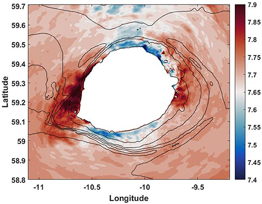
Figure 5. The model predicted temperature at the depth of 1,000 m after 144 h of model time.

Note that the analytical solution presented above was developed for a two-dimensional topography. It can also be applied for the qualitative analysis of the bottom trapped waves considered in our case. In doing so, the solution was replicated for four transects shown in Figure 6E. Figures 6A–D demonstrate the analytical results for each transect separately. The analytical solution shows that the maximum of horizontal velocity in all positions is located below 1,000-m depth, Figures 6A–D. This theoretical result is consistent with Figure 2 where in-situ recorded data reveal the great intensity of horizontal velocities at the bottom.

FIGURE 6

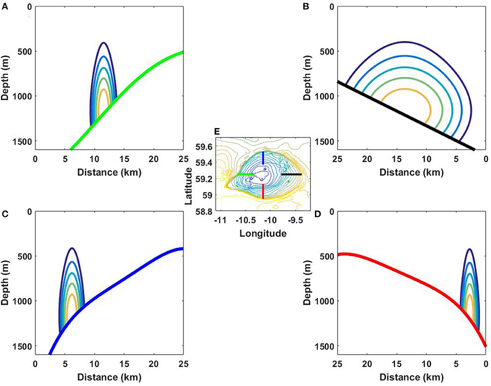
Figure 6. Zero-mode normalized eigenfunctions of the boundary value problem (3)–(4) calculated for the bottom transects (A–D) shown by the same color in (E).

The power spectra calculated using a 144-h model predicted time series of horizontal velocity (the sampling interval was equal to 1 min) also reveal the maximum for bottom-located baroclinic tidal motions in the position of all CTD stations, Figure 7. The data set contains only the internal wave signal extracted after the removal of barotropic velocity. Figure 7 illustrates the predominance of the semidiurnal tidal signal. Note that 6- and 3-h harmonics are also evident in all graphs. Their peaks are comparable to the semidiurnal signal or even higher in the energy level (station 31), which testifies the strong non-linearity of the internal wave process. Such waves will increase the mixing process that can contribute to better larvae dispersion (van Harren et al., 2014; Cyr et al., 2016). A general tendency of all graphs is that the energy level at the bottom and in the surface layer (red and blue lines in Figure 7, respectively) substantially exceeds a similar level calculated for the mid-depth segments (green-yellow colors). This fact confirms the hypothesis of two internal waveguides separated by a less active intermediate layer.

FIGURE 7

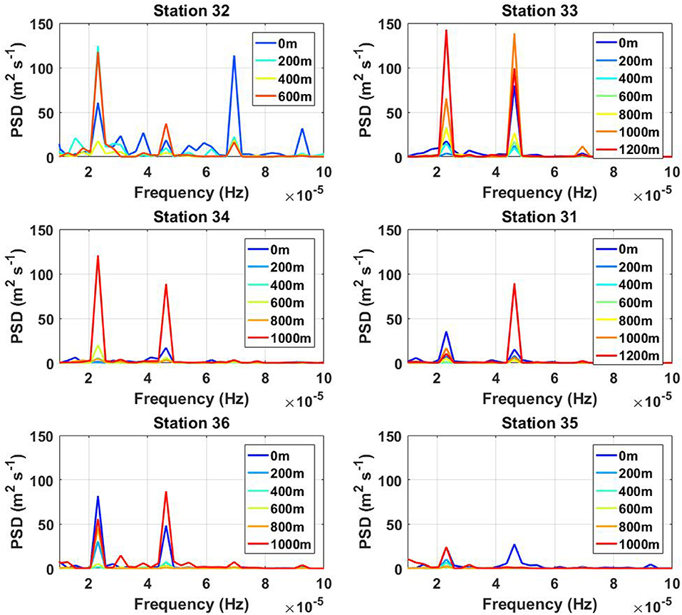
Figure 7. The model predicted power spectra density calculated for all stations.

4.2. Waves in the Surface Layer

The summit of RBS has a group of parasitic volcanic cones, Figure 8A. Water depth at the highest cone is about 300 m (Howe et al., 2006). The interaction of tidal currents with cones can generate internal lee waves in sharp seasonal pycnocline. If this statement is correct, the phase speed c of internal waves in the area of volcanic cones should be comparable or lower than the maximum of tidal velocity U. In other words, the Froude number Fr = U/c should be close or exceed one. Below we estimate the maximum of the Froude number.

FIGURE 8

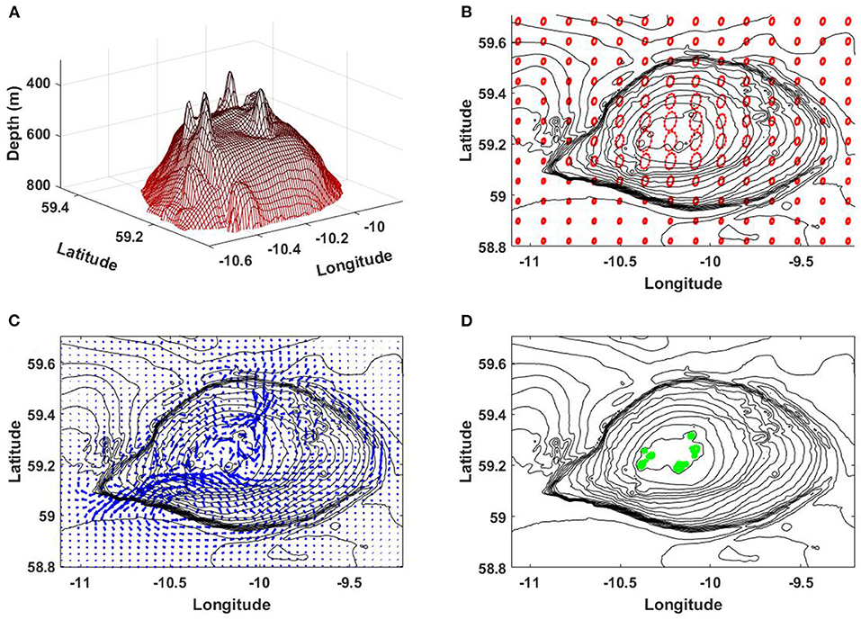
Figure 8. (A) Bathymetry of RBS above 800 m depth. (B) Tidal ellipses in the RBS area predicted by the TPXO8.1 tidal model. (C) The model predicted residual currents. (D) The green color shows the positions with the Froude number Fr > 1.

The periodic tidal currents, together with tidally induced residual currents, control the dynamical regime around RBS. According to TPXO8.1 model predictions, tidal velocities above the RBS summit can reach 0.35 m s⁻¹ (see tidal ellipses in Figure 8B). The residual currents calculated using long-term velocity time series show the maximum value of 0.11 m s⁻¹, Figure 8C. Superposition of both can give 0.46 m s⁻¹ maximum value of the velocity U at some moments of tidal phase.

The phase speed of short-scale internal waves c was found from the boundary value problem (Benny, 1966):

$\begin{array}{l}{w}_{zz}+\frac{N^2(z)}{c^2}w=0,\\ w(-H)=w(0)=0.& (6)\end{array}$

Here w is the vertical velocity. Solution of (6) was found by shooting method, that gave the first eigenvalue c =0.36 m s⁻¹. The estimation of the Froude number shows that it slightly exceeds one in the area of the cones, i.e., Fr > 1, Figure 8D. Thus, the generation of internal lee waves at the cones explains the presence of short-scale internal waves over RBS, Figure 3. The area occupied by these groups of short waves above RBS over one tidal period is shown in Figure 9A. This pattern presents a superposition of hourly recorded amplitudes of horizontal velocity $\sqrt{u^2+v^2}$ taken over one tidal cycle overlaid in one plot. The dark red curved stripes depict the wavefronts of internal waves (horizontal velocities) at the free surface. The shape of wavefronts, their orientation, and their spatial position suggests that these waves propagate to the northeast and southwest. They are generated above volcanic cones according to the lee-wave mechanism. The areas with Fr > 1 are colored in yellow in Figure 9A.

FIGURE 9

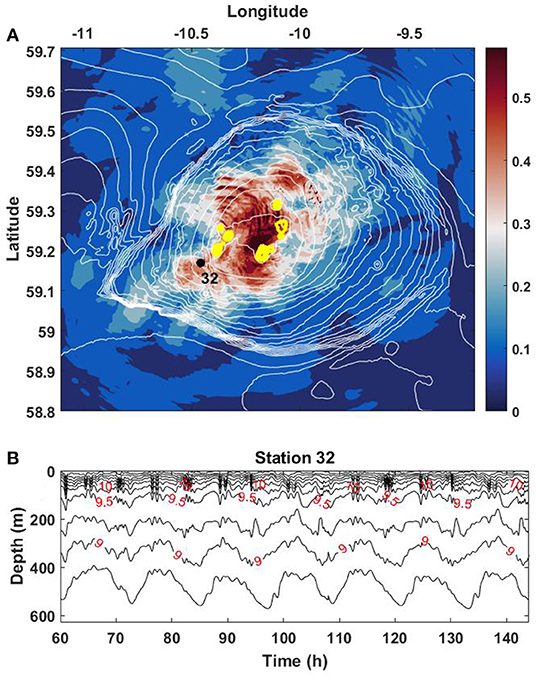
Figure 9. (A) Hourly model outputs of the horizontal velocity amplitude $\sqrt{u^2+v^2}$ (ms⁻¹) at the free surface for one tidal period overlaid in one plot. The volcanic cones are depicted in yellow color. (B) The model predicted temperature time series at station 32. The red labels on isotherms are given in ^oC.

Using the model-predicted time series of temperature recorded with 1-min sampling interval at the position of station 32, Figure 9B, one can estimate the vertical structure and temporal variability of these short-scale internal waves generated over volcanic cones. It is clear from Figure 9B that the internal wave packets occupy mostly surface 100 m thick layer, i.e., the seasonal pycnocline. The intensity of short-scale waves below this level is much lower. As a confirmation, analysis of in-situ recorded vertical profiles shown in Figure 2 reveals the same tendency, i.e., a higher level of intensity of horizontal velocities in the upper surface layer at all stations.

Evidence of lee wave generation in the surface layer is demonstrated here for summer conditions. The internal wave dynamics in the area are controlled by water stratification, which varies from season to season. Figure 10 shows that the water stratification in the surface layer is quite sensitive to the seasonal variability. The surface layer is well stratified during summer and almost homogeneous in winter. The buoyancy frequency profiles shown in Figure 10 were calculated for the RBS area using monthly averaged temperature and salinity data sets based on 94 CTD stations (Levitus and Boyer, 1994). It is expected that the seasonal variability of the fluid stratification can modify the internal wave dynamics over RBS. Note that the fluid stratification below 400 m depth is relatively conservative and does not reveal any essential seasonal variability. The surface seasonal pycnocline does not exist from November to March, but the main pycnocline is relatively stable over the whole year. One can assume that no internal wave activity in the surface layer can be expected during the winter season, but it can be pretty active in the summertime.

FIGURE 10

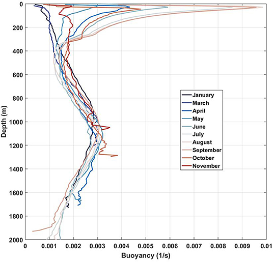
Figure 10. Monthly averaged buoyancy frequency profiles for the RBS area.

Thus, one can assume that during winter, the water dynamics over RBS are controlled by the bottom trapped sub-inertial internal waves. Surface internal waves that are active under summer conditions can not affect the deep-water coral dispersion during the wintertime, controlled by bottom trapped internal waves.

5. Larvae Dispersion

Together with the in-situ data, the modeling experiments reveal two types of internal waves generated by tidal currents over the RBS summit. The short-scale internal waves, Figure 9B are located in the surface stratified layer (seasonal pycnocline, Figure 1C). The bottom sub-inertial trapped internal waves are concentrated in the area of the main pycnocline below 600 m depth. Both types of waves can produce water mixing that supplies nutrients and food for deep-water corals and facilitate coral larvae dispersion (Mohn et al., 2014; Cyr et al., 2016).

Numerically wise, having a model velocity as a background process, one can estimate all possible ways of deep-water coral larvae transport around RBS using a Lagrangian approach. A trilinear interpolation with 5-min velocity model outputs was used in these experiments (for the details, see Supplementary Material, the Lagrangian model.) This method can help in understanding to what extent the cloud of larvae released over the bank disperse and escape from RBS.

We consider the larvae as particles with zero buoyancy. Strömberg and Larsson (2017) studied the swimming behavior of the larvae in laboratory tanks. They found that the larvae can move along spirals in circles rather than bullet-style swimming. Considering the larvae trajectories, they look like a Brownian chaotic motion without preferential directions. So, in this paper, we decided to consider the larvae as passive particles. In doing so, 11,000 particles were seeded uniformly on the RBS summit. The experiments were restricted by 1,400 m depth. The spatial step between the position of the released particles was 450 m. The output model velocities were used as an input data set for the Lagrangian-type passive particle tracking model (Stashchuk et al., 2018) to reproduce the pathway of larvae from their initial position. In setting the time scale for the larvae spreading experiments, we followed the results of Larsson et al. (2014) who showed that 50 days is the most real lifetime for larvae to be dispersed.

The results of the 50 days passive tracer experiments are summarized in Figure 11. It was found that the particles disperse differently in different directions depending on their initial position at the RBS summit. Four groups of particles can be classified based on the analysis of their tracks:

• (i) particles that lifted to the surface above 300 m depth;

• (ii) the group of particles that migrated over the summit but always remained within the bank area;

• (iii) the particles that leave the RBS summit and propagate northward;

• (iv) the group of particles that leave RBS and propagate to the west.

FIGURE 11

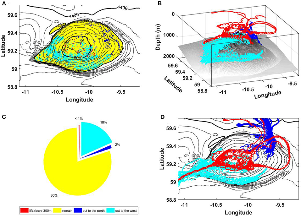
Figure 11. (A) Initial position of particles lifted to the surface (red), transported from RBS northward (blue), advected to the west of the bank (cyan), and migrated over the RBS summit (yellow). Particle tracks in three dimensions (B), and their plan view from the above (D). (C) Percentage of particles in the considered groups. The colors of particle groups in all sub-plots coincide.

The initial position of these four groups of particles is shown in Figure 11A. The color is used to mark the particle of the same group: red for the group (i), yellow for the group (ii), blue for the group (iii), and cyan for the group (iv).

Technically, it is impossible to show the trajectory of all 11,000 particles seeded on RBS in one plot. Instead, we demonstrate here only some typical scenarios of evolution showing their tracks in three dimensions, Figure 11B, or presenting the plan view of the particle trajectories, Figure 11D. The pie-plot, Figure 11C, summarizes the specific weight of every particular group (percentage calculated from the total amount). The larvae population lifted to the surface (red color), and those leaving the bank in the northern direction (blue color) are the smallest. The vast majority of particles migrate over the summit without leaving the seamount. Quite a remarkable number of larvae (at least 18%) could escape from RBS propagating to the west.

Interestingly, all particles which propagated vertically to the surface were located initially at the top of RBS, Figure 11A. Their ascent can be associated with vertical motions induced by the generated internal waves. Taking into account the seasonal variability of water stratification in the RBS area, Figure 9, one can conclude that this mechanism of larvae dispersion is possible only at summertime when seasonal pycnocline is developed. Statistically, most particles propagate horizontally by the residual currents associated with the bottom trapped internal waves. The main pycnocline is stable during all seasons, so one can conclude that this mechanism is active over the whole year.

Samples of two different coral species, Lophelia pertusa and Madrepora oculata, were collected and filmed during a series of JC136 ROV dives. In the North Atlantic, Lophelia pertusa spawns once a year between January and March, when two waveguides do not exist. However, Madrepora oculata spawns twice a year (Waller and Tyler, 2005), and vertical motion may influence the larvae dispersion. This circumstance should be taken into account considering possible scenarios of larvae dispersal, Figure 11, applying them to different types of deepwater corals.

6. Discussion and Summary

The great importance of seamounts for cold-water coral connectivity in the North Atlantic was acknowledged in many papers (e.g., Fox et al., 2016). The significant effect of internal tides for the coral larvae dispersion was also confirmed by Vlasenko et al. (2018) who numerically quantified the tidally-driven larvae transport in the area of Anton Dohrn Seamount. One of the ideas reported recently is that global-scale modeling can predict the deep-water coral larvae spreading. Ross et al. (2020) discussed the global scale effect of coral larvae dispersion in the North Atlantic estimating the connectivity between different coral communities. In this study, the larvae transport was modeled using a Lagrange passive tracer model. The oceanic background currents were taken from the output of two large-scale hydrodynamic models, HYCOM (Black, 2002) and POLCOMS (Holt and James, 2001). The aim was to estimate the ways of larvae transport in the North Atlantic over several months. Their study revealed a very great sensitivity of the larvae dispersion trajectories to the model grid scales. Specifically, the uncertainty of hydrodynamic model predictions could result in contrasting ecological interpretations. The principal conclusion of this paper was that high-resolution modeling is required for making more robust predictions.

In this context, the high-resolution modeling of tidal action, as presented in this paper, is quite efficient for describing the local dynamics and larvae spreading. Such an approach we used considering coral larvae dispersion over two seamounts in the NE Atlantic, ADS (Stashchuk et al., 2018; Vlasenko et al., 2018) and RBS (reported in the present paper). These two oceanic banks, RBS, and ADS are located at a distance 170 km (Figure 1A). They are quite different in form. ADS is a table-bank formation with very abrupt slopes. RBS has a Gaussian-type shape. It is more massive in size and contains several tall, steep volcanic cones on its summit. As a result of different geometrical forms, these two seamounts reveal quite different internal wave dynamics. Specifically, this concerns the internal tides generation mechanisms. ADS reveals evidence of internal tidal beams radiated from the flanks of the seamount focusing on the central part over the topography. The synthesis of observational data and modeling results confirms the beam structure of internal tides over ADS. A variety of short-scale internal wave motions is produced by the tidal beams hitting the seasonal pycnocline over the ADS summit (Stashchuk et al., 2018; Vlasenko et al., 2018).

The structure of the tidally generated internal waves in the RBS area is quite different. First of all, no internal tidal beams were recorded over RBS in observations. The numerical experiments also confirmed the same result. The bottom currents intensification recorded experimentally at the CTD stations is explained here in terms of the bottom trapped internal wave theory discussed above. The second difference between the internal wave dynamics is the generation of short-wave internal waves over RBS. The existence of tall volcanic cones over the RBS summit creates the conditions for the generation of short internal waves in the seasonal pycnocline according to the lee-wave mechanism. That is not the case with ADS, so the larvae dispersion in these two areas is different. In any case, internal wave activity in both areas is a good source of nutrients and organic matter supply for coral communities, White and Dorschel (2010).

The larvae transport depends on the residual currents that are formed by tides around seamounts. In the ADS area, such currents produce four eddies, Vlasenko et al. (2018); Stashchuk et al. (2018). They provide four main directions for possible larvae trajectories: westward, southward, northward, and northeastward. Thus, potentially, the coral larvae from ADS can reach RBS and deposit there. As distinct from ADS, in the RBS area, only two eddies are formed by the tidal currents. Figure 8C shows possible larvae tracks, mostly in northern and westward directions, without any chance to settle at ADS. These modeling results indicate possible connectivity between ADS and RBS that is controlled by tides.

For both seamounts, ADS, and RBS, the coral larvae were considered purely passive initially. However, taking into account their possibility to swim (Larsson et al., 2014) the initial position of the particles was 5-m above the bottom.

The model prediction time of larvae dispersion in the present paper is based on the results reported by Larsson et al. (2014). In their laboratory investigations of embryogenesis and larval development of cold-water coral Lophelia pertusa have shown that nematocysts appear when larvae are 30 days old. After this time, they can settle and give rise to a new coral colony. We have used a planktonic larval duration of 50 days. That is close to 43 days reported by Hilário et al. (2015) as the mean minimum duration for eurybathic species.

The principal outcomes can be summarized as follows:

• Internal wave dynamics

Barotropic tide generates two types of internal waves over RBS. Long-scale semidiurnal internal waves are active below 800 m depth in the layer of the main pycnocline. Their spatial structure is well described by a zero-eigenfunction of the boundary value problem (4). The maximum velocity of this function is located at the bottom.

Short-scale internal waves occupy mostly surface 100-m layer. They can be registered only during the warm season when the seasonal pycnocline exists. These short internal waves are generated by the tidal flow interacting with a cluster of narrow, tall bottom cones, Figure 8A that has a volcanic origin. The conditions for the generation of these short internal waves, Figure 9, is supercritical in terms of the Froude number, Fr. Specifically, these waves are excited when Fr > 1. These surface layer short-period internal waves can be classified as unsteady lee waves.

• Deep water biological communities

The internal tides developing in the RMS area can have a significant implication on deep-water coral populations. The larvae live in the water column for more than a month and move with currents before settling down in a new area. The deep-water transport produced by internal tides is one of the principal drivers for coral dispersion (Henry et al., 2014). In this study, we show that the deep-water dynamics over the RMS summit are controlled by bottom trapped internal waves that can initiate residual currents transporting the larvae similar to the mechanism described in Stashchuk et al. (2018). The modeling results help in understanding the larvae transport, i.e., how far the particles can migrate from their initial positions, Figure 11.

Data Availability Statement

The datasets presented in this study can be found in online repositories. The names of the repository/repositories and accession number(s) can be found below: https://figshare.com/articles/RBS/11688990. More details on the 136th cruise of the RRS “James Cook” can be found at https://deeplinksproject.wordpress.com/ and inventories/cruise_inventory/report/16050.

Author Contributions

All authors listed have made a substantial, direct and intellectual contribution to the work, and approved it for publication.

Funding

This work was supported by the UK NERC grant NE/K011855/1.

Conflict of Interest

The authors declare that the research was conducted in the absence of any commercial or financial relationships that could be construed as a potential conflict of interest.

Publisher's Note

All claims expressed in this article are solely those of the authors and do not necessarily represent those of their affiliated organizations, or those of the publisher, the editors and the reviewers. Any product that may be evaluated in this article, or claim that may be made by its manufacturer, is not guaranteed or endorsed by the publisher.

Acknowledgments

The authors would like to thank the captain, the crew, and scientific team working together during the JC136 cruise in 2016. The authors appreciate also the collaboration with the University of Plymouth High Performance Cluster team.

Supplementary Material

The Supplementary Material for this article can be found online at: https://www.frontiersin.org/articles/10.3389/fmars.2021.735358/full#supplementary-material

References

Bell, D. J. (1975). Topography generated internal waves. J. Geophys. Res. 80, 320–327. doi: 10.1029/JC080i003p00320

CrossRef Full Text

Benny, D. J. (1966). Long nonlinear wave in fluid flows. J. Math. Phys. 25, 241–270. doi: 10.1017/S0022112066001630

CrossRef Full Text | Google Scholar

Black, R. (2002). An oceanic general circulation model framed in hybrid isopycniccartesian coordinates. Ocean Model. 4, 55–88. doi: 10.1016/S1463-5003(01)00012-9

CrossRef Full Text | Google Scholar

Cyr, F., van Haren, H., Mienis, F., Duineveld, G., and Bourgault, D. (2016). On the influence of cold water coral mound size on flow hydrodynamics, and vice versa. Geophys. Res. Lett. 43, 775–783. doi: 10.1002/2015GL067038

CrossRef Full Text | Google Scholar

Dale, A. C., Huthnance, J. M., and Sherwin, T. J. (2001). Coastal-trapped internal waves and tides at near-inertial frequencies. J. Phys. Oceanogr. 31, 2958–2970. doi: 10.1175/1520-0485(2001)031andlt;2958:CTWATAandgt;2.0.CO;2

CrossRef Full Text | Google Scholar

Davison, J. J., van Haren, H., Hosegood, P., Piechaud, N., and Howell, K. L. (2019). The distribution of deep-sea sponge aggregations (porifera) in relation to oceanographic processes in the faroe-shetland channel. Deep Sea Res. I 146, 55–61. doi: 10.1016/j.dsr.2019.03.005

CrossRef Full Text | Google Scholar

de Mol, B., van Rensbergen, P., Pillen, S., van Herreweghe, K., van Rooij, D., McDonnell, A., et al. (2002). Large deep-water coral banks in the porcupine basin, southwest of ireland. Mar. Geol. 188, 193–231. doi: 10.1016/S0025-3227(02)00281-5

CrossRef Full Text | Google Scholar

Egbert, G. D., and Erofeeva, S. Y. (2002). Efficient inverse modeling of barotropic ocean tides. J. Atmos. Oceanic Technol. 19, 183–204. doi: 10.1175/1520-0426(2002)019andlt;0183:EIMOBOandgt;2.0.CO;2

CrossRef Full Text | Google Scholar

Fox, A. D., Henry, L. H., Corne, D. W., and Robberts, J. M. (2016). Sensitivity of marine protected area network connectivity to atmospheric variability. R. Soc. Open Sci. 3:160494. doi: 10.1098/rsos.160494

PubMed Abstract | CrossRef Full Text | Google Scholar

Henry, L.-A., Vad, J., Findlay, H. S., Murillo, J., Milligan, R., and Roberts, J. M. (2014). Environmental variability and biodiversity of megabenthos on the hebrides terrace seamount (northeast atlantic). Sci. Rep. 4:5589. doi: 10.1038/srep05589

PubMed Abstract | CrossRef Full Text

Hilário, A., Metaxas, A., Gaudron, S., Howell, K. L., Mercier, A., Mestre, N. C., et al. (2015). Estimation dispersal distance in the deep sea: challenges and applications to marine reserves. Front. Mar. Sci. 2:6. doi: 10.3389/fmars.2015.00006

CrossRef Full Text | Google Scholar

Holt, J. T., and James, I. D. (2001). An s-coordinate density evolving model of the north west european continental shelf. part 1. model description and density structure. J. Geophys. Res. 106, 14015–14034. doi: 10.1029/2000JC000304

CrossRef Full Text | Google Scholar

Howe, J. A., Stoker, M. S., Masson, D. G., Pudsey, C. J., Morris, P., Larter, R. D., et al. (2006). Seabed morphology and the bottom-current pathways around Rosemary Bank seamount, northern Rockall Trough, North Atlantic. Mar. Petroleum Geol. 23, 165–181. doi: 10.1016/j.marpetgeo.2005.08.003

CrossRef Full Text | Google Scholar

Huthnance, J. M. (1978). On coastal trapped waves. analysis and numerical calculations by inverse iterations. J. Phys. Oceanogr. 8, 74–92. doi: 10.1175/1520-0485(1978)008andlt;0074:OCTWAAandgt;2.0.CO;2

CrossRef Full Text | Google Scholar

Larsson, A., Järnegren, J., Strömberg, S., Dahl, M. P., Lundälv, T., and Brooke, S. (2014). Embryogenesis and larval biology of the cold-water coral Lophelia pertusa. PLoS ONE 9:e102222. doi: 10.1371/journal.pone.0102222

PubMed Abstract | CrossRef Full Text | Google Scholar

LeBlond, P., and Mysak, L. (1978). Waves in the Ocean. Amsterdam; Oxford; New York, NY: Elsevier.

Google Scholar

Levitus, S., and Boyer, T. P. (1994). World Ocean Atlas 1994. Washington, DC: US Government Printing Office.

Google Scholar

Marshall, J., Adcroft, A., Hill, C., Perelman, L., and Heisey, C. (1997). A finite-volume, incompressible Navier-Stokes model for studies of the ocean on parallel computers. J. Geophys. Res. 102, 5733–5752. doi: 10.1029/96JC02776

CrossRef Full Text | Google Scholar

Mohn, C., Rengstorf, A., White, M., Duineveld, G., Mienis, F., Soetaert, K., et al. (2014). Linking bentic hydrodynamics and cold-water coral occurances: a high-resolution model study at three cold-water coral provinces in the ne atlantic. Progr. Oceanogr. 122, 92–104. doi: 10.1016/j.pocean.2013.12.003

CrossRef Full Text | Google Scholar

Mohn, C., and White, M. (2010). Seamounts in restless ocean: response of passive tracers to sub-tidal flow variability. Gephys. Res. Lett. 37:L15606. doi: 10.1029/2010GL043871

CrossRef Full Text | Google Scholar

Pacanowski, R. C., and Philander, S. G. H. (1981). Parameterisation of vertical mixing in numerical models of Tropical Oceans. J. Phys. Oceanogr. 11, 1443–1451. doi: 10.1175/1520-0485(1981)011andlt;1443:POVMINandgt;2.0.CO;2

CrossRef Full Text | Google Scholar

Roberts, J. M., Wheeler, A. J., and Freiwald, A. (2006). Reefs of the deep: the biology and geology of cold water coral ecosystems. Science 312, 543–547. doi: 10.1126/science.1119861

PubMed Abstract | CrossRef Full Text | Google Scholar

Ross, R. E., Nimmo-Smith, W. A. M., Torres, R., and Howell, K. L. (2020). Comparing deep-sea larval dispersal models: s cautionary tale for ecology and conservation. Front. Mar. Sci. 12:431. doi: 10.3389/fmars.2020.00431

CrossRef Full Text | Google Scholar

Soetaert, K., Mohn, C., Rengstorf, A., Grehan, A., and van Oevelen, D. (2016). Ecosystem engineering creates a direct nutritional link between 600-m deep cold-water coral mounds and surface productivity. Sci. Rep. 6:35057. doi: 10.1038/srep35057

PubMed Abstract | CrossRef Full Text | Google Scholar

Stashchuk, N., and Vlasenko, V. (2017). Bottom trapped internal waves over the Malin Sea continental slope. Deep Sea Res. I 119, 68–80. doi: 10.1016/j.dsr.2016.11.007

CrossRef Full Text | Google Scholar

Stashchuk, N., Vlasenko, V., Hosegood, P., and Nimmo-Smith, A. W. M. (2017). Tidally induced residual current over the malin sea continental slope. Cont. Shelf. Res. 139, 21–34. doi: 10.1016/j.csr.2017.03.010

CrossRef Full Text | Google Scholar

Stashchuk, N., Vlasenko, V., and Howell, K. L. (2018). Modelling tidally induced larval dispersal over Anton Dohrn Seamount. Ocean Dyn. 68, 1515–1526. doi: 10.1007/s10236-018-1206-0

CrossRef Full Text | Google Scholar

Stashchuk, N., Vlasenko, V., Inall, M. E., and Aleynik, D. (2014). Horizontal dispersion in shelf seas: high resolution modelling as an aid to sparse sampling. Progr. Oceanogr. 128, 74–87. doi: 10.1016/j.pocean.2014.08.007

CrossRef Full Text | Google Scholar

Strömberg, S. M., and Larsson, A. I. (2017). Larval behavior and longevity in the cold-water coral Lophelia pertusa indicate potential for long distance dispersal. Front. Mar. Sci. 12:411. doi: 10.3389/fmars.2017.00411

CrossRef Full Text

van Harren, H., Mienis, F., Duineveld, G. C. A., and Laveleye, M. S. S. (2014). High-resolution temperature observations of trapped nonlinear diurnal tide influencing cold-water corals on the logachev mounds. Progr. Oceanogr. 125, 16–25. doi: 10.1016/j.pocean.2014.04.021

CrossRef Full Text | Google Scholar

van Weering, C. E., de Haas, H., de Stigter, H., Lykke-Anderson, H., and Kouvaev, I. (2003). Structure and development of giant carbonate mounds at the sw rockall trough margins, ne atlantic ocean. Mar. Geol. 198, 67–81. doi: 10.1016/S0025-3227(03)00095-1

CrossRef Full Text | Google Scholar

Visbeck, M. (2002). Deep velocity profiling using lowered acoustic doppler current profilers: bottom track and inverse solutions. J. Atmos. Oceanic Tech. 10, 794–807. doi: 10.1175/1520-0426(2002)019andlt;0794:DVPULAandgt;2.0.CO;2

CrossRef Full Text

Vlasenko, V., and Stashchuk, N. (2018). Tidally induced overflow of the faroese channels bottom water over the Wyville Thomson Ridge. J. Geophys. Res. 123, 6753–6765. doi: 10.1029/2018JC014365

CrossRef Full Text | Google Scholar

Vlasenko, V., and Stashchuk, N. (2021). Setting tidal forcing for numerical modelling of internal waves. Ocean Model. 160:101767. doi: 10.1016/j.ocemod.2021.101767

CrossRef Full Text | Google Scholar

Vlasenko, V., Stashchuk, N., Inall, M. E., and Hopkins, J. (2014). Tidal energy conversion in a global hot spot: on the 3-D dynamics of baroclinic tides at the Celtic Sea shelf break. J. Geophys. Res. 119, 3249–3265. doi: 10.1002/2013JC009708

CrossRef Full Text | Google Scholar

Vlasenko, V., Stashchuk, N., Inall, M. E., Porter, M., and Aleynik, D. (2016). Focusing of baroclinic tidal energy in a canyon. J. Geophys. Res. 121, 2824–2840. doi: 10.1002/2015JC011314

CrossRef Full Text | Google Scholar

Vlasenko, V., Stashchuk, N., and Nimmo-Smith, W. A. M. (2018). Three dimensional dynamics of baroclinic tides over a seamount. J. Geophys. Res. 123, 1263–1285. doi: 10.1002/2017JC013287

CrossRef Full Text | Google Scholar

Vlasenko, V., Stashchuk, N., Palmer, M., and Inall, M. E. (2013). Generation of baroclinic tides over an isolated underwater bank. J. Geophys. Res. 118, 4395–4408. doi: 10.1002/jgrc.20304

CrossRef Full Text | Google Scholar

Waller, R. G., and Tyler, P. A. (2005). The reproductive biology of two deep-water, reef-building scleractinians from the ne atlantic ocean. Coral Reefs. 24, 514–522. doi: 10.1007/s00338-005-0501-7

CrossRef Full Text | Google Scholar

Wang, D.-P., and Mooers, C. N. K. (1976). Coastal-trapped waves in a continuously stratified. J. Phys. Oceanogr. 6, 853–863. doi: 10.1175/1520-0485(1976)006andlt;0853:CTWIACandgt;2.0.CO;2

CrossRef Full Text | Google Scholar

White, M., and Dorschel, B. (2010). The importance of the permanent thermocline to the cold water coral carbonate mound distribution in the ne atlantic. Earth Planet Sci Lett. 296, 395–402. doi: 10.1016/j.epsl.2010.05.025

CrossRef Full Text | Google Scholar

Willmott (1981). On the validation of models. Phys. Geogr. 2, 184–194. doi: 10.1080/02723646.1981.10642213

CrossRef Full Text | Google Scholar

Willmott (1982). On the climatic optimization of the tilt and azimuth of flat-plane solar collectors. Solar Energy. 28, 205–216. doi: 10.1016/0038-092X(82)90159-1

CrossRef Full Text | Google Scholar