The Influence of the River Discharge on Residence Time, Exposure Time and Integrated Water Fractions for the Tagus Estuary (Portugal)

Understanding how long water is retained in an estuary and how quickly it is completely flushed is essential to estimate an estuary’s health in areas with significant pollutant loadings. The present study analyses the effect of five different Tagus River discharge scenarios ranging from low to extreme on residence time (RT), exposure time (ET) and integrated water fractions inside pre-established Tagus estuary areas, to identify its most vulnerable areas to pollution. The 3D version of the MOHID hydrodynamic model coupled to a lagrangian tool was used. The increase of the river discharge generated high current velocities which, in turn, led to an increased rate of tracers leaving the estuary. As a consequence, RT and ET decreased from 59 to 3.5 days under a low and extreme river discharge scenario, respectively. Under a low river discharge, significant differences were observed between RT and ET in the areas located in the main body of the estuary and in the bays. As river discharge increased, RT and ET decreased in all areas of the estuary and those differences faded, with the greatest differences observed in the areas situated along the south margin. In general, results showed that with high river discharges the tracers released in the upper estuary are spread throughout the estuary, but mainly in downstream areas. However, when the river discharge reached exceptionally high values, local eddies were formed, leading to the retention of the tracers in the estuary’s south margin and inner bays. The results in this study allowed to identify the most vulnerable areas within the estuary as a function of the river discharge.

Introduction

Estuaries are transition zones characterized by salinity and nutrient gradients generated by the mixing between freshwater from rivers and saltwater from oceans. Large residence times and nutrients availability place them amongst the most productive aquatic environments on Earth and are a habitat of many aquatic species. The rate of water exchange between an estuary and the adjacent coast regulates the physical, chemical, and biological processes within the basin (Yuan et al., 2007; Cloern et al., 2017; Raimonet and Cloern, 2017).

Estuaries are habitat to many species because water renewable time scale is larger than the timescale associated to phytoplankton development, allowing phytoplankton biomass to support secondary producers. This capacity turns out to be a problem when the natural system is disturbed by anthropogenic loads. In this case, a short renewable time scale is convenient, making some regions more appropriate for receiving anthropogenic discharges than others. However, the complexity of the transport processes makes ranking the ability of each region to receive anthropogenic discharges difficult, creating conditions for the definition of several timescales which suitability depends on the local dynamics and modeling tools available. Water age, flushing time, residence time, exposure time, and transit time are concepts used to describe water exchange, sometimes in a confusing way. Bolin and Rodhe (1973) published a paper clarifying the meaning of age, turn-over (also called flushing time) and residence time, popular during the sixties. Later on, Zimmerman (1976) published a paper on the same subject, addressing the concept of transit time and its relationship with age and residence time. Since those times, many others addressed this issue (Matso, 2018; Dippner et al., 2019). During these 50 years the technological evolution was huge and ecosystem models based on high resolution hydrodynamic models are now able to individualize the contribution of particular loads on the properties of the ecosystem, and Lagrangian models enable tracking of the trajectory of tracers released in particular locations and instances and quantify the interaction between different zones of the estuary (Braunschweig et al., 2003). However, the need for integrated (over time) values that are easy to assess, and the understanding of their connection to the river discharge is still needed to understand the biological functioning of the estuary and the most suitable locations for anthropogenic discharges.

Amongst these, residence time (RT) and exposure time (ET) are the most useful descriptors to estimate the mixing and renewal of estuarine waters (Zhang et al., 2010; Xiong et al., 2021) and, therefore, to understand estuarine dynamics. RT of a water parcel is an integrative parameter that measures the renewal time for a given water parcel or water body (Defne and Ganju, 2015) and is defined as the time the water will spend in the domain of interest until leaving it for the first time. Nevertheless, in oscillatory flows (e.g., tidal estuaries) the water may leave and return several times. To account for the effects of the return flow, the concept ET was introduced as an alternative to RT (Monsen et al., 2002; Delhez et al., 2004), and is defined as the amount of time a water parcel spends in a particular zone until it never returns. Based on these definitions, it can be concluded that at a given time and location, ET is always larger than, or equal to, RT. Therefore, large differences between the two timescales indicate that part of the water tends to return more often to the domain of interest after leaving it for the first time, than when the differences are smaller. Both RT and ET are important descriptors of the estuarine behavior (Takeoka, 1984; Delesalle and Sournia, 1992; de Brauwere et al., 2011; Sun et al., 2014) because they represent the time scale of the physical transport processes (Zimmerman, 1976; Takeoka, 1984), and because they can be compared with time scales of biochemistry fluxes and processes (Jay et al., 1997; Lucas and Deleersnijder, 2020).

Estuarine hydrodynamics, RT, and ET vary in both space and time (Zhang et al., 2010; Azhikodan and Yokoyama, 2016; Bárcena et al., 2016). The combined effects of several meteoceanographic drivers (tides, riverine flows and meteorological data, such as wind) and estuarine geomorphology shape the hydrodynamics, RT and ET on timescales ranging from hours to months (Bárcena et al., 2012; Defne and Ganju, 2015; Xiong et al., 2021). Understanding how long water is retained in an estuary and how quickly water is flushed from the water body is essential to ascertain the health vulnerability of the estuary in areas with significant pollutant loadings (Bárcena et al., 2017a).

Yuan et al. (2007) stated that a pollutant exerts most of its effects if its biochemical timescales are equal to, or lower than, the RT. For instance, RT is related to estuarine eutrophication (Tapia González et al., 2008), a phenomenon widely recognized as a major worldwide threat (Valiela et al., 1997), generated from excessive amounts of nutrients in the aquatic system (Bricker, 1999). Areas with long RT tend to retain nutrients and promote higher primary productivity rates, whereas areas with reduced RT tend to disperse nutrients due to the water exchange with adjacent, less impacted, coastal waters (Defne and Ganju, 2015). According to Zhang and Wang (2012), algae blooms could be inhibited if the RT of nutrients is less than the doubling time of algae cells in the estuary. Timescales for the transport processes have several applications, such as the transport of nutrients from sewage treatment plants (Signell et al., 2000), the export of copepod life stages (Ohman and Wood, 1996), the dispersion of floating debris (Kako et al., 2014; Jambeck et al., 2015; Kooi et al., 2018), the occurrence of harmful algal blooms (Bricelj and Lonsdale, 1997), the degree of water exchange in heavily modified water bodies (Gómez et al., 2014), the prediction of the location of oil from oil spills (Spaulding, 2017), bacterial loading (Yu et al., 2021), amongst others. Therefore, the knowledge of the spatiotemporal RT and/or ET distribution is paramount to identify the most sensitive areas in vulnerability assessment studies (Duarte et al., 2002; Cavalcante et al., 2012; Bárcena et al., 2017b).

Residence time and ET can be estimated for the whole estuary or only for a few areas of it. Indeed, for management purposes it is important to divide the estuary into small areas based on their morphology and hydrodynamics, as well as local drivers, as these will influence the water renewal time of specific areas in a different way. Therefore, spatiotemporal differences of RT and ET should be considered in the decision-making process. Apart from the determination of water timescales for each area, it is also important to understand the history of water renewal in those areas, which is named integrated water fraction (Braunschweig et al., 2003). This allows understanding how water from different areas interact with each other, and how the dispersion of tracers occurs within the estuary.

In the present study, RT and ET were studied for the Tagus estuary, the most extensive estuary of the Iberian Peninsula located in a highly populated region subject to both natural and human pressures. The RT for the Tagus estuary was previously studied by Oliveira and Baptista (1997) and Braunschweig et al. (2003). The former authors used particle tracking models to analyze RT based on integral methods. However, this approach fails to accurately describe the dynamics between different water masses within the estuary. The latter authors used a Lagrangian transport model coupled to a 2D hydrodynamic model (2D–MOHID), whose depth integrated configuration affects the residual transport and, therefore, the renewal time scales (Braunschweig et al., 2003). To overcome this issue, this work uses the 3D version of the MOHID hydrodynamic model, coupled to a Lagrangian transport module to estimate RT and ET within the estuary, and to investigate the history of the integrated water fractions by considering the water exchange over time between areas within the estuary. Moreover, the meteoceanographic data used varied in time instead of being considered constant as applied in the previously cited studies.

Five river discharges scenarios were analyzed, ranging from low to extreme discharges, with the objective of predicting the possible pollutant effects in the water body based on RT, ET and integrated water fractions, essential to optimize the management of the Tagus estuary.

The present work aimed to answer the following questions: (i) How does river discharge influence RT and ET within the estuary?; (ii) How are tracers dispersed within the estuary according to their origin?; (iii) How are water exchanges among different areas of the estuary?; (iv) Which estuarine areas are more vulnerable to pollutants?

Materials and Methods

Study Area

The study area is located in the Portuguese west coast (30.6° N–9.5° W) and comprises a ROFI zone (Region of Freshwater Influence) that embraces the Tagus estuary (Figure 1). This estuary occupies a volume of 1.9 × 10⁹ m³ with a surface area of approximately 320 km² (Valente and da Silva, 2009; Guerreiro et al., 2015). It is part of the transnational Tagus River basin, covering an area of about 80,800 km² [APA, (Agência Portuguesa do Ambiente), 2015]. The estuary is pear-shaped with roughly 30 km long and presents a complex morphology that can be divided into three distinct zones: upstream area, middle area, and external area (Neves, 2010; Rusu et al., 2011). In its upstream area, the estuary connects with the river through a channel of 200 m width. This area is characterized by a low average depth of around 2 m and presents most of the mudflats, the salt marshes, and the islands formed by alluvial deposition in the estuary. The middle area is the largest of the estuary with 15 km wide and with an average depth of about 7 m. In this area there are two important bays (Montijo and Seixal) presenting a complex and branched morphology, whose waters extend inland, and where intertidal flats dominate. Finally, in the external area, the estuary connects to the Atlantic Ocean, through a deep, long and narrow channel with 12 km length, 2 km wide and a maximum depth of 40 m (Fortunato et al., 1997).

FIGURE 1

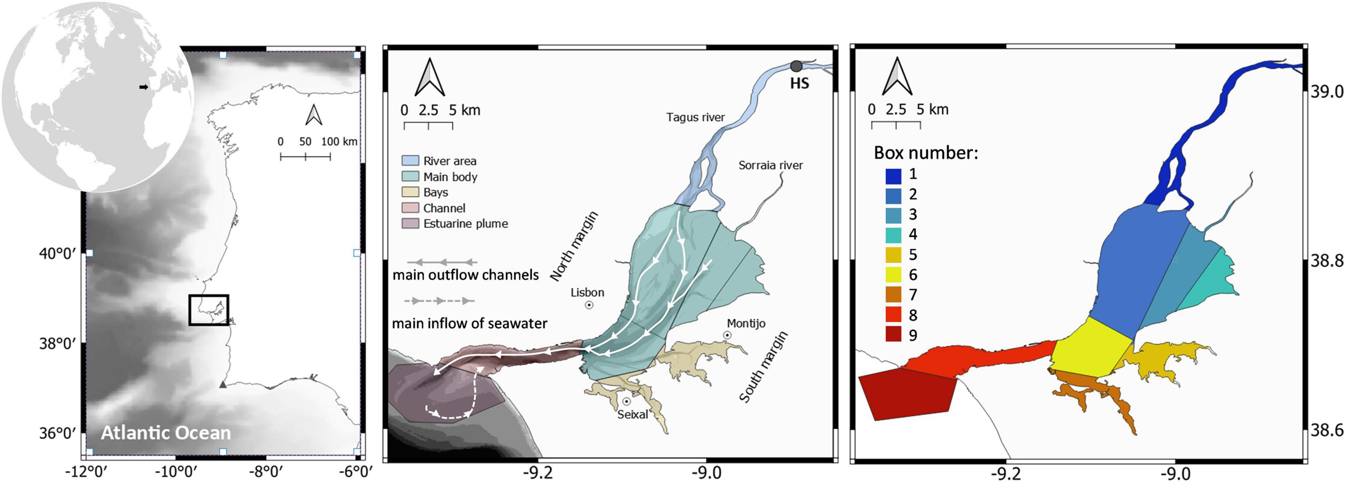
Figure 1. Maps showing the TagusROFI (square; left); Designations used in the present work and bathymetry–darker colors represent higher depths (middle); and boxes used to calculate residence time, exposure time and integrated water fraction (right). HS–Hydrological Station.

The Tagus estuary is a semidiurnal, mesotidal and, usually, well-mixed estuary, presenting at the river mouth an average tidal amplitude of 2.4 m. According to Gameiro et al. (2007), the tidal range varies between 0.9 and 4.1 m during neap tides and spring tides, respectively. Furthermore, due to the large extent of the tidal flats that occupy 40% of the estuary, the estuary is strongly ebb-dominated (Fortunato et al., 2017). The tidal amplitude and the river inflows are mainly responsible for the mixing processes within the estuary. Data obtained between 2006 and 2019 from the Almourol hydrological station, located in the Tagus River (Figure 1), indicated that the river discharge varied from 0 to 9,874 m³/s (instantaneous measurements), with an annual average river discharge of 263 m³/s. River discharge influences water levels until 40 km upstream of the estuarine mouth (Vargas et al., 2008), whilst, downstream, tide and storm surge drive water levels. Although tides are the main driver of the estuarine circulation, other forces may also influence the estuarine hydrodynamics, namely riverine flow (Rodrigues et al., 2019), meteorological processes, and the nonlinear interactions with bathymetry and morphology.

Model Setup

In this work an online coupling between the 3D-MOHID Water eulerian model and the MOHID lagrangian model in its particle-tracking form were used. The coupling between these two models is one directional, where information is transferred from the eulerian model to the lagrangian model, which uses the eulerian velocity fields to track the displacement of lagrangian particles.

The 3D-MOHID Water eulerian model solves the primitive continuity and momentum equations for the surface elevation and 3D velocity field, in orthogonal horizontal coordinates and generic vertical coordinates, applied to an Arakawa-C type grid. Hydrostatic equilibrium, Boussinesq approximations and incompressible flow assumptions are considered, and the finite volume approximation is used to discretize the equations. Time discretization is done with an Alternate Direction Implicit (ADI) scheme, and the available advection schemes include the first, second and third order upwind numerical schemes by centered differences and/or the Total Variation Diminishing (TVD).

The present study uses the 3D baroclinic application of MOHID Water eulerian model for the estuarine area of the TagusROFI which considers both tidal and density driven currents. Bathymetry was built by integrating data from the General Bathymetric Chart of the Oceans (GEBCO) and from the Hydrographic Institute (Figure 1). The model domain has a horizontal grid step that varies between 200 m and in the vertical direction has 7 sigma layers from the surface followed by 43 cartesian Z level layers. Results from the Portuguese Coast Operational Modeling System (PCOMS), whose implementation is described by Campuzano et al. (2016), were used as the open sea boundary condition (velocities, surface elevation, temperature and salinity) on a one-way downscaling method. A flather radiation scheme (Flather, 1976) was then combined with a flow relaxation scheme for the first 10 numerical boarder cells with a decay time of 1 week to obtain a stable and smooth solution. A biharmonic coefficient of 10⁶ m⁴ s^–2 was used to reduce high frequency noise generated inside the domain and advection was computed using the TVD advection scheme. Atmospheric forcing was provided by the Weather Research and Forecasting (WRF) meteorological model with a 3 km spatial resolution (Trancoso, 2012), and it was interpolated to the TagusROFI domain. River discharges (Tagus, Trancão, and Sorraia) in the TagusROFI domain were imposed as volume discharges (without momentum). The Tagus River discharge was registered at the hydrological station and obtained from the National Water Resources Information System (SNIRH) with a frequency of 1 h. For the other rivers (Trancão and Sorraia) data were imposed using climatological values, with river discharges ranging between 1 and 9 m³ s^–1 for the Trancão River, and 3 and 60 m³ s^–1 for the Sorraia River. Monthly climatological values of freshwater temperature and salinity for the three rivers and for water discharges from 14 wastewater treatment plants (WWTPs) were also imposed. For a detailed description of the model implemented see de Pablo et al. (2019) and Sobrinho et al. (2021).

Concerning the validation of the eulerian field, specifically for the present domain, Portela and Neves (1994) compared model predictions with the water surface elevation obtained from a tide gauge located inside the estuary (Cabo Ruivo; 38.75°N; −9.09°W), as well as suspended particulate matter data measured in situ. The results achieved by these authors were consistent with observations and with previously knowledge about the estuary. Vaz et al. (2011), compared harmonic analysis results of measured and model predicted sea surface height for 12 stations covering the whole estuary, and found a good correlation between observations and predictions. Franz et al. (2014) also reported a good correlation between model results and the current velocity measured during 6 months with an ADCP located in the central body of the estuary (38.73°N; −9.05°W). More recently, de Pablo et al. (2019) validated the hydrodynamic model for the Tagus ROFI. These authors to validate the water level, compared data obtained from the Lisbon tide gauge (38.71° N; −9.13° W) with model predictions and determined a correlation coefficient of 0.994, an average BIAS of 0.005 and root mean square error of 0.45. In the same paper, salinity and temperature data from a CTD located in the estuary channel was used to validate model results. Those authors also found a good fit between measurements and model predictions for these variables.

As opposed to the Euler method, the Lagrangian tracer method does not compute fluxes across the faces of a finite volume but rather transports tracers due to a gridded velocity field computed by an Euler method (in this case by the 3D-MOHID Water eulerian model), whose field velocities are interpolated into a new grid with a resolution that is set by the user with the sole purpose of obtaining a higher resolution velocity field. To address the motion of tracers, we consider them as ideal pointwise particles and eulerian velocities are interpolated in time and space to each tracer particle. The equation of motion that describe the particle trajectory is:

$\frac{d{x}_i}{dt}=v_i(x_i\left(t\right),t)+D_i(1)$

Where v_i is the velocity of the flow field at a time instant t and D_i is the velocity due to diffusion. The horizontal diffusion term (Equation 2) is modeled using random velocities while the tracer travels a given mixing length, proportional to the resolution of the flow velocity field v_i(x_i(t),t) (and its ability) to resolve motion scales.

$D_i=R\cdot \sqrt{\frac{2k_h}{dt}},t(2)$

Where K_h is the current diffusivity vector. To compute K_h, we consider it as a linear relation of the current particle velocity, K_h=K⋅_vk, where K is the diffusion coefficient and it is set K=1 (m² s^–1), a value used in constant anisotropic diffusion models, and v_k=v_i/v_l is an non dimensional factor used to weight the diffusion factor with the current particle velocity v_i. R is a random number generated at each time step in each direction, with an average value of 0.0 and standard deviation of 1.0.

To ensure that diffusion mainly contributes to the motion of tracers where the resolution of the underlying current velocity field is not able to resolve motion of short scales lower than the model output, we constraint the update of D_i in Eq. 2 to the condition of the traveled distance due to diffusion is higher than the model resolution 2⋅Δ_{xy},

${\mathbf{\text{D}}}_{\mathbf{i}}\cdot dt<2\cdot {\mathrm{\Delta }}_{\left\{xy\right\}}(3)$

This approach ensures that a particle keeps with the same stochastic diffusion velocity noise while it remains in the same neighboring area (< 2⋅Δ_{xy}), and it is updated when it travels to a new region in the flow field (>2⋅Δ_{xy}).

Lagrangian tracers can be emitted at a point, on a line or on a polygon defined in space. They can be emitted as an instantaneous release, continuously over time or within a specified time interval included in the simulation time. In the present work, the Lagrangian tracers were distributed in a grid of 200 m × 200 m × 1 m, injected in the initial simulation time (t₀), in nine polygons that correspond to the nine monitoring boxes, the target of this study. With this methodology, around 180 thousand conservative particles were released uniformly into de estuary. All tracers maintain their initial identity which in this case corresponds to the monitoring boxes (sources) where they were distributed.

Determination of Residence Time, Exposure Time and Integrated Water Fractions

The present work follows the methodology proposed by Braunschweig et al. (2003), which consists in dividing the estuary into 2D vertically integrated boxes. In this case, the Tagus estuary was divided into 9 boxes (Figure 1) that were defined based on the existing knowledge regarding hydrodynamics, morphology, and biogeochemical characteristics of the system. Box 1 comprises the most upstream area of the Tagus River. Boxes 2 to 4 and box 6 are in the central body of the estuary. Boxes 5 and 7 cover the Montijo and Seixal bays, respectively. Box 8 covers the channel that connects the estuary to the Atlantic Ocean, and Box 9 is located near the estuarine mouth in the region of the estuarine plume influence. The sum of the partial volume of each box corresponds to the total estuarine volume. All boxes were used as releasing areas of the Lagrangian tracers (monitoring boxes), which allowed the identification of the tracers’ source. At the same time, the boxes were used to understand the spatial and temporal distribution of the tracers within the estuary for monitoring purposes. Since each tracer is identified by its source, it is possible to determine the water exchange among boxes (integrated water fractions) during the simulations.

The variation of the number of tracers within a box over time is given by the following equation:

$\mathbf{\text{f}}(\mathbf{t})=\frac{{\mathbf{\text{N}}}_{\mathbf{i}}(\mathbf{t})}{{\mathbf{\text{N}}}_{\mathbf{i}}({\mathbf{\text{t}}}_{\mathbf{0}})}(4)$

Where N_i(t) is the number of tracers from the box i at time t, whereas N_i(t₀) is the number of tracers in box i at time t₀.

For each box, RT should be estimated as the time that all tracers needed to leave it for the first time, whereas ET should be estimated as the time elapsed until all the tracers of that box were replaced by new water. However, this would lead to unrealistic RT and ET estimations and thus RT and ET (named as hydrodynamic indicators in this study) should be considered attained when a certain number of residual tracers are still in the area under study (Braunschweig et al., 2003).

If it is assumed that a known concentration of particles is injected into the estuary at a given time (t = 0) an initial concentration (C₀) is obtained, and if no further particles are loaded after t = 0 and the volume of the estuary remains constant over time, the concentration within the estuary at a given time, C(t), can be calculated using a decreasing exponential function:

$\mathbf{\text{C}}\left(\mathbf{t}\right)={\mathbf{\text{C}}}_{\mathbf{0}}.{\mathbf{\text{e}}}^{-\mathbf{t}/\mathbf{RT}},\mathrm{where}\mathrm{RT}\mathrm{is}\mathrm{the}\mathrm{residence}\mathrm{time}(5)$

From this equation (5) it can be seen that at time t = RT the concentration decreased to e^–1, i.e., to 37% of the initial concentration. The residence time is then defined by the time required to decrease the fraction of particles in the estuary to 37% of its original value (100%). This, however, is only true for diffusive systems. In systems where advective processes are also relevant, such as the present study area, this approximation cannot be applied in the strict sense. There is no consensus in the literature about the criterion to be used to define the proportion of the residual tracers from which the RT and ET is attained in distinct areas (Huang et al., 2011). In the present work, for the whole estuary and for each box, RT is reached when 80% of the tracers has left the box for the first time and ET was considered achieved at the time when the number of tracers in the box never exceeds 20%. This threshold was kept constant for all boxes and case studies which allowed the comparison of the results.

Residence time and ET do not consider the history of the water renewal process. Thus, the number of tracers from box j at time t₀ located inside box i were integrated in time, following the expression:

${\mathbf{\text{F}}}_{\mathbf{i},\mathbf{j}}\left(\mathbf{t}\right)=\frac{\mathbf{1}}{\mathbf{\text{T}}}{\int }_{\mathbf{0}}^{\mathbf{T}}\frac{{\mathbf{\text{N}}}_{\mathbf{i},\mathbf{j}}\left(\mathbf{t}\right)}{{\mathbf{\text{V}}}_{\mathbf{i}}\left(\mathbf{t}\right)}\mathbf{\text{dt}}\mathit{\hspace{1em}\hspace{0.25em}}\mathbf{i},\mathbf{j}:\mathbf{1}\mathrm{\dots }\mathrm{\dots }\mathbf{9}\mathit{\hspace{1em}\hspace{0.5em}}\mathbf{t}:\mathbf{0}\mathrm{\dots }..\mathrm{\infty }(6)$

Where T corresponds to the simulation time (in the present study, 1 week) and F_i,j(t) represents the fraction of tracers from box j in the box i at time t, V_i(t) is the volume of box i over time (which changes with tide), and N_i,j(t) is the number of tracers from the box i at time t.

Case Studies

In the present work, five case studies with different river discharge rates were chosen, based on a 13-year time series (2006–2019) of the Tagus River discharge obtained every 15 min from the hydrological station (Figure 2). Case studies 1, 2 and 3 reflect low (summer typical situation), mean and high river discharges (occurring mainly during the winter), respectively, while case studies 4 and 5 represent two extreme events observed during the studied period (Figure 2). The main meteoceanographic conditions simulated for each case study are summarized in Table 1 and are represented in Figure 3. The discharge rates observed for each case study were implemented in the 3DMOHID Water eulerian model which produced the field velocities used by the particle-tracking model. In addition, all simulations started at ebb tidal phase.

FIGURE 2

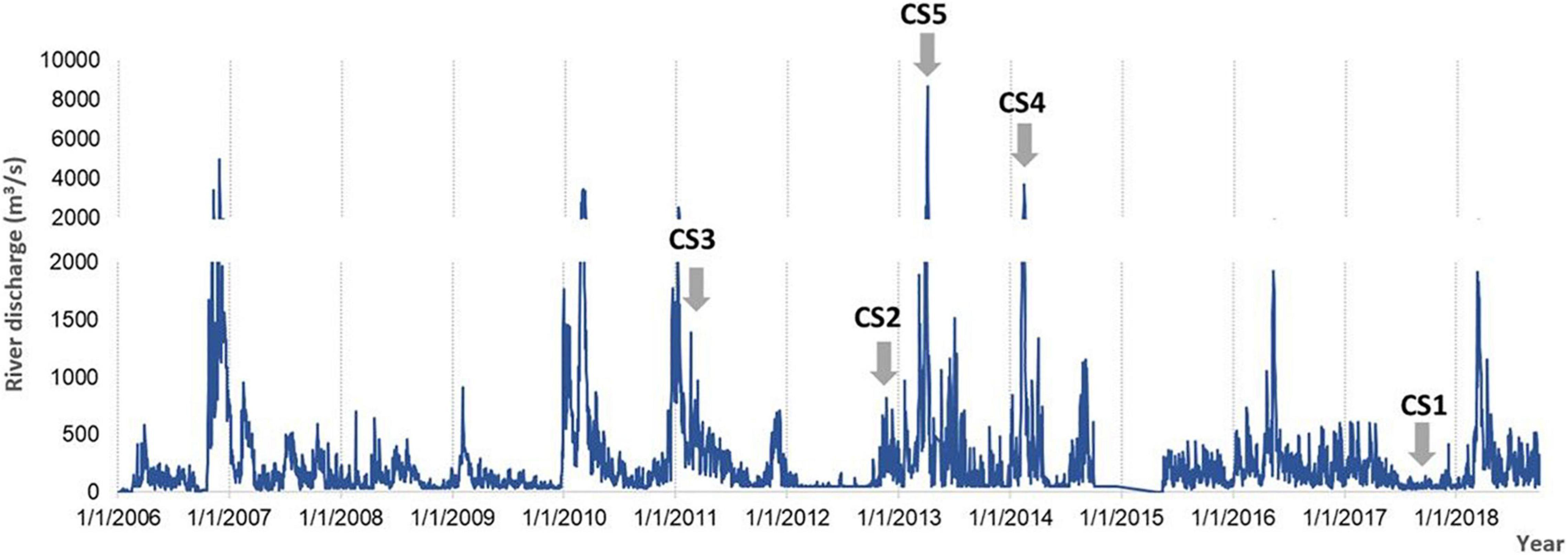
Figure 2. Daily average of the Tagus River discharge between 2006 and 2019 with indication of the case studies period.

TABLE 1

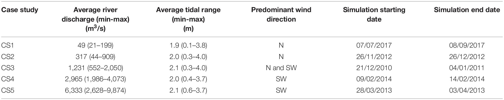
Table 1. Summary of the conditions simulated for each case study.

FIGURE 3

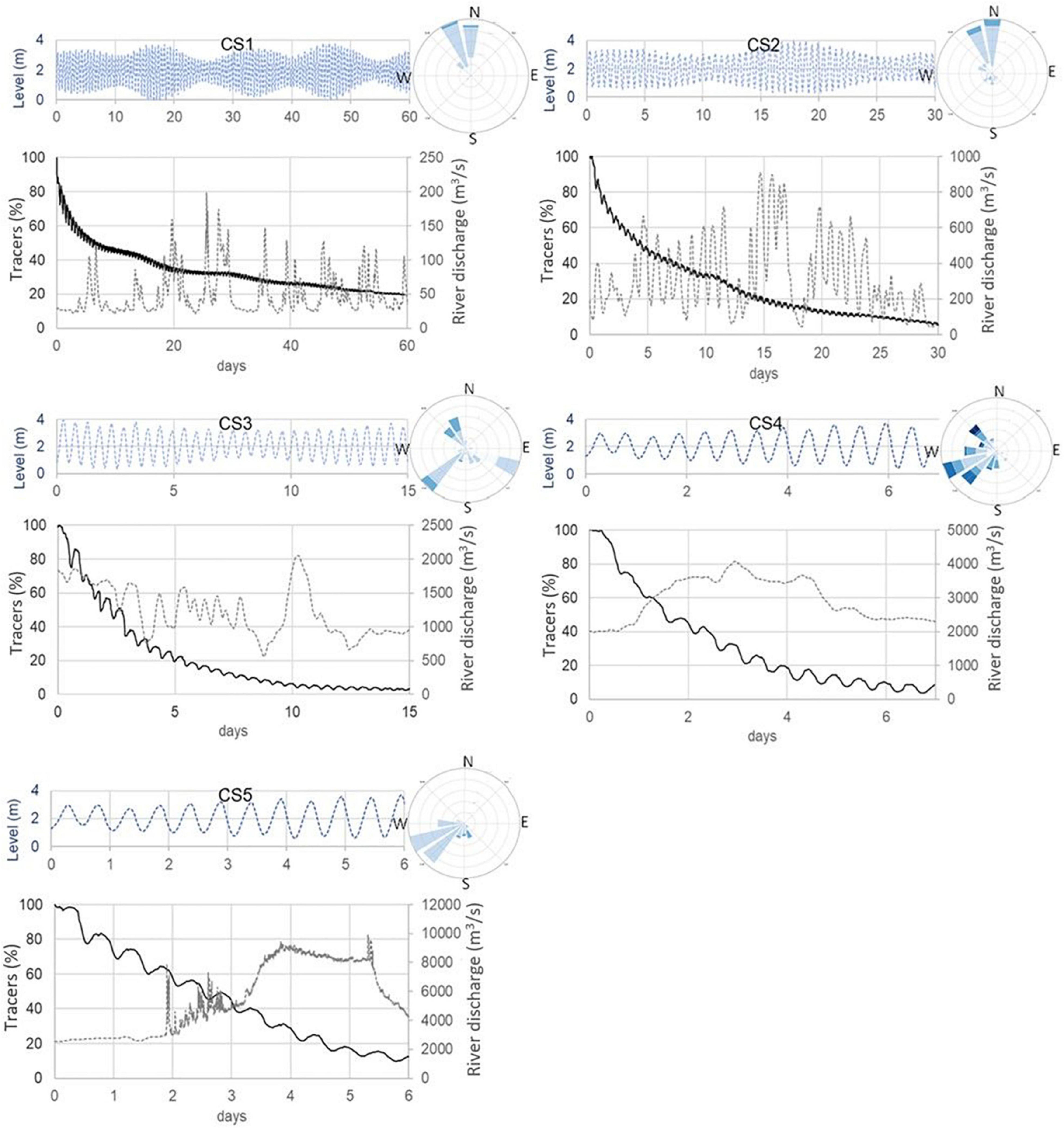
Figure 3. Variation of the proportion of initial tracers over time determined for the whole Tagus estuary and for the five case studies. Real time metocean data (wind, river discharge, and water level) observed during the studied period are also presented.

Results

Residence Time and Exposure Time

Real time input data observed during the studied period, as well as the percentage of tracers inside the estuary over time determined for the whole Tagus estuary and for the five case studies are shown in Figure 3. RT was achieved when the proportion of the initial tracers reached the 20% line for the first time, whilst ET was achieved when the proportion of tracers inside the estuary dropped below the 20% line (in comparison with the initial state) and did not go up the 20% line again. The simulations were carried out until 80% of the tracers had moved to the shelf. For all case studies half of the initial tracers were lost within the first week of simulation, independently of the river discharge (6.6, 4.5, 2.3, 1.5, and 2.5 days for CS1, 2, 3, 4, and 5, respectively). No significant differences were observed between RT and ET for the entire estuary, and for the five case studies (Figure 3). The highest and lowest value for all case studies were determined for CS1 (59 days) and CS4 (3.5 days), respectively. For CS2, 3 and 5 these hydrodynamic indicators values were 15, 5.5, and 4.5 days, respectively (Figure 3). For CS1 the river discharge was always lower than 200 m³/s and the wind was weak. Similar metocean conditions were observed for CS2 and 3, but with a higher river discharge in CS3 where the highest river discharge registered reached 909 m³/s. For CS4, apart from the river discharge, which remained above 2,000 m³/s during the studied period, high wind intensities were observed. On the contrary, for the most extreme river discharge (CS5), wind conditions were weak during the simulation period (Figure 3). Regarding wind direction, in CS3 to 5 winds prevailed from southeast, a typical situation of the raining season in this area. The tide level variation was identical for all case studies and covered at least part of a neap tide and a spring tide.

The values of RT and ET obtained for the different case studies can be related to the river discharge in order to derive an inverse variation function (Figure 4). This allowed the estimation of the RT and ET as a function of the Tagus River discharge. By the analysis of Figure 4, large variations can be observed of both RT and ET between low (CS1) and medium river discharges (CS2), while between medium and extreme mean river discharges (CS2 to 5) these hydrodynamic indicators varied only slightly. Nevertheless, it is interesting to note that in the most extreme river discharge event (CS5), RT and ET increased slightly when compared with high river discharges (CS3 and 4) indicating that the water currents resulting from those extreme events promoted the retention of tracers within certain areas of the estuary (Figure 4).

FIGURE 4

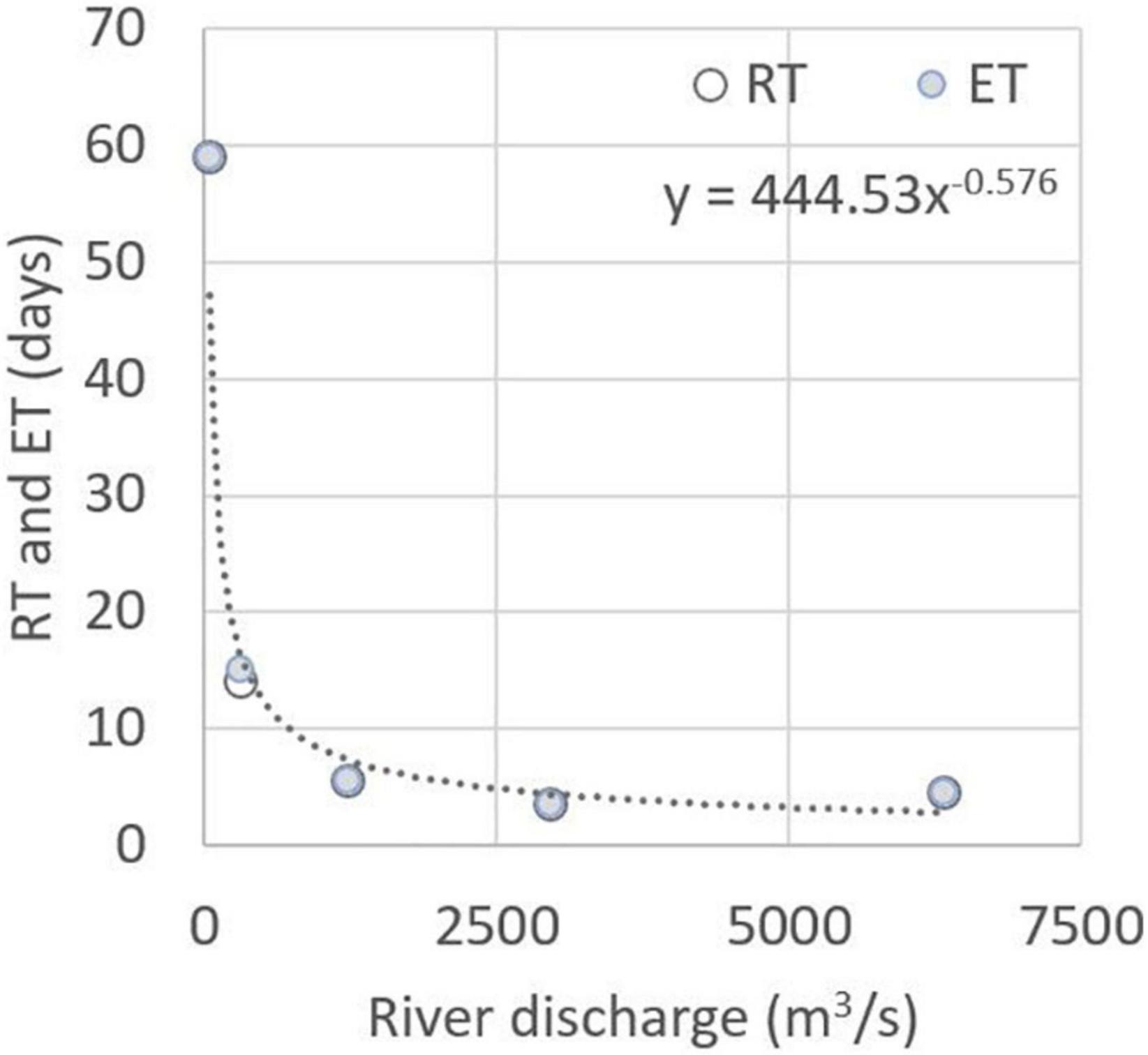
Figure 4. Variation of RT and ET (days) in function of the river discharge (m³/s).

From a management point of view, it is paramount to determine both RT and ET for different areas of the estuary since hydrodynamics in these areas is also influenced by both local bathymetry and morphology. With this purpose, the studied area was divided into 9 boxes. In general, the calculated RT showed a similar trend for all boxes and for CS1 to 4, that is, this indicator decreased with the increase of the river discharge. Furthermore, the RT obtained for boxes 6, 8, and 9 was always low (less than 2 days) regardless of the river discharge, with the lowest value observed for box 6 (less than 6 h for all case studies) (Figure 5).

FIGURE 5

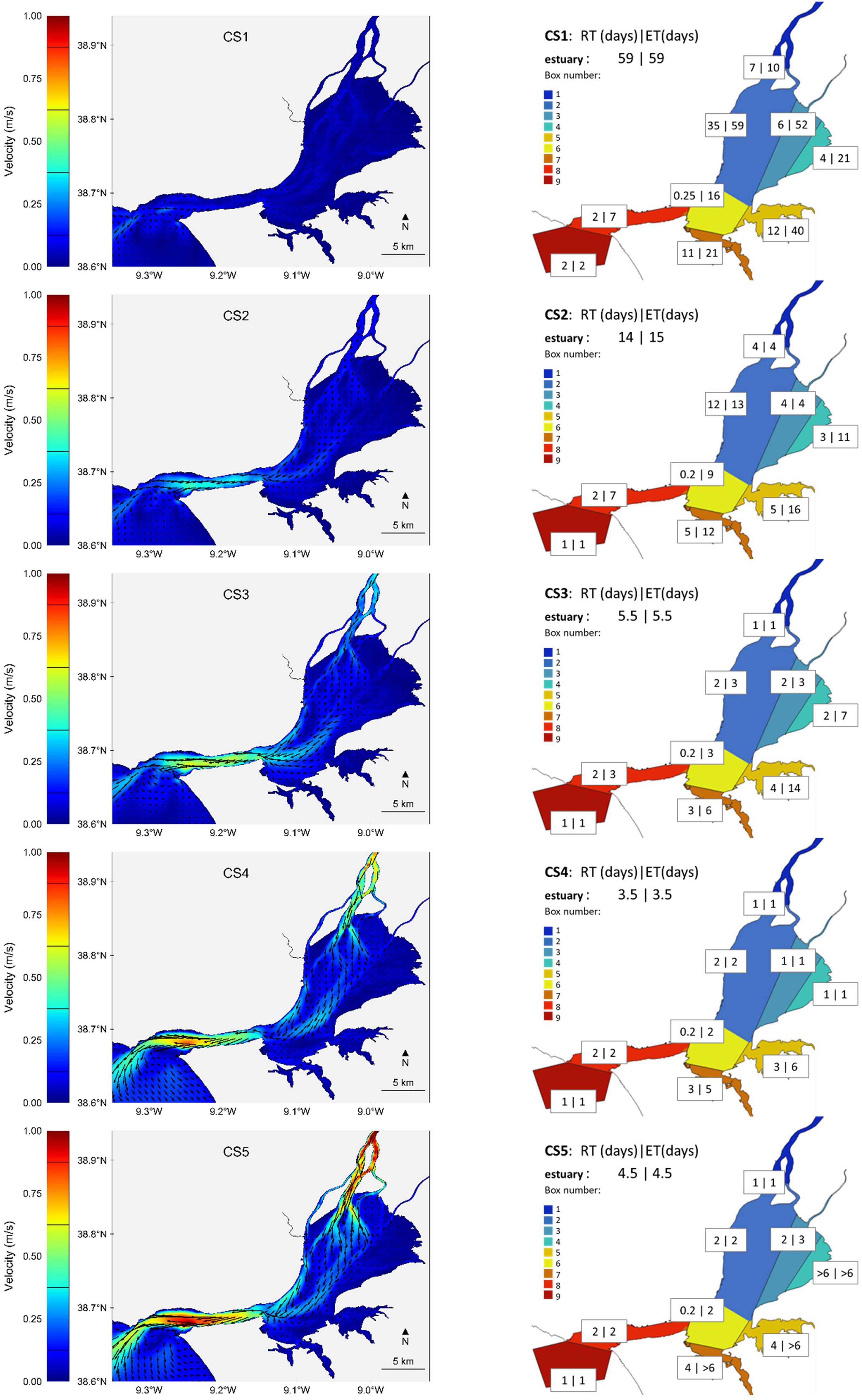
Figure 5. Left: Mean velocity, intensity and direction of the currents in the Tagus estuary for each case study; Right: RT and ET determined for each box and case study.

Regarding the RTs determined for CS1, it was observed that this indicator was higher in box 2 (35 days) located in the main body of the estuary, followed by the boxes that comprise the Montijo (box 5; 12 days) and Seixal (box 7; 11 days) bays (Figure 5). Boxes 1, 3, and 4 that comprehend the most upstream area of the estuary and also the remaining part of its main body, presented lower RTs, (7, 6, and 4 days, respectively). Although with lower RTs due to the increase of current velocity generated by the increase of the river discharge, the results obtained for CS2 were similar to those described for CS1 (Figure 5). In CS3 and CS4, characterized by high and extreme river discharges, respectively, the RTs determined for both the most upstream area (box 1) and main body of the estuary (boxes 2 to 4) decreased significantly when compared with the RTs determined for these boxes in CS1 and CS2. Indeed, in CS3 and CS4, the RT observed for those boxes ranged between 1 and 2 days, a much lower value than the ones obtained for CS1 and CS2 (Figure 5).

Concerning ET, Figure 5 shows that the lower values were always determined for box 9, located in the most downstream area of the estuary, and corresponding to the estuarine plume, an area highly influenced by coastal circulation. In this area the calculated ET was 2 days for the lowest river discharge (CS1) and 1 day for the remaining case studies. In the most upstream area (box 1) the influence of the tide was only noted for low (CS1) and medium (CS2) river discharges with ET reaching 10 and 4 days, respectively. At mean river discharges higher than 1,231 m³/s an ET of 1 day was obtained for this box. Box 8 corresponds to the channel that connects the main body of the estuary with the estuarine plume area. From Figure 5 it can be observed that for low (CS1) and mean (CS2) river discharges an ET of 7 days was achieved, whilst for higher river discharges the ET decreased to 3 for CS3 and 2 days for CS4 and CS5. The main differences observed for the first 4 case studies were mainly observed in both the main body of the estuary and in the bays (boxes 2 to 7) (Figure 5). CS1, when the mean river discharge is low (summer condition), presented the highest ET values determined. In this case study, and for boxes 2 to 7, the ET ranged between 16 and 59 days, with the highest values registered in boxes 2 (59 days) and 3 (52 days), both located in the main body of the estuary. For CS2, 3 and 4, ET decreased with the increase of the river discharge, with the highest ET achieved in box 7 (16, 14, and 6 days, respectively) (Figure 5). CS5 corresponds to the most extreme event studied. The results of RT and ET achieved for boxes 1, 2, 6, 8, and 9 and for this case study showed that the tracers were rapidly flushed away from the estuary, reaching equal values of RT and ET obtained in these areas for CS4. However, in the remaining boxes (3, 4, 5, and 7), both descriptors increased comparatively to CS4 (Figure 5).

Figure 6 illustrates the location of the tracers at different tidal instances and for all boxes over a period of about two first tidal cycles of the CS2 simulation (medium river discharge) which represents the most frequent Tagus River discharge. This figure represents all the tracers released in the water column and not only the tracers that remained in the surface layer of water. It can be observed that the tracers launched in box 2 were mainly transported along their source box (around 15 km length) and for high periods of time (associated to the tidal cycle). This explains why the RT and ET values determined for this area were high and similar across case studies. Regarding boxes 4, 5 and 7, characterized by low current velocities, the tracers released in each of them were retained for a longer period of time, leaving those boxes very slowly throughout the simulation time, leading to high values of ET. During the flood tide, tracers from box 8 progressed into the estuary but only until the middle of the central body and along its north margin (box 2). Finally, is interesting to note that the higher concentrations of tracers from box 9 were observed in deeper layers which is in accordance with the hydrodynamics of the estuary related to the entrance of salt water in it.

FIGURE 6

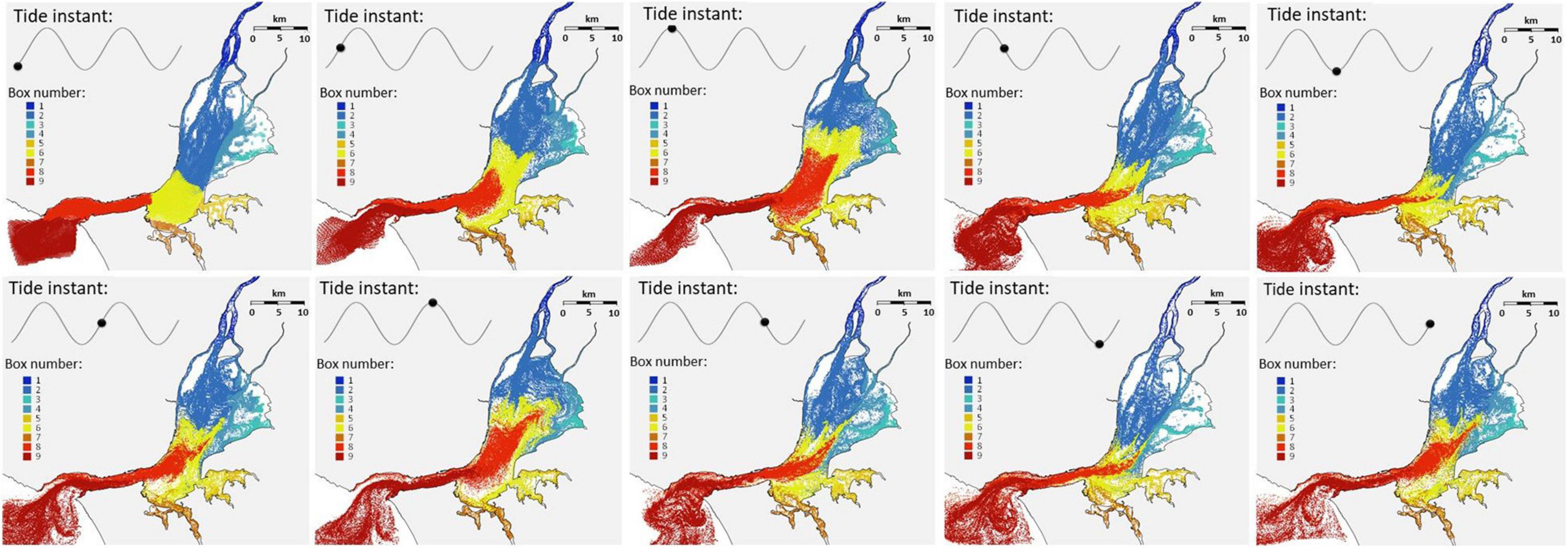
Figure 6. Location of the tracers at different tidal points and for all boxes over about two first tidal cycles of the simulation and for the CS2 (medium river discharge).

Integrated Water Fraction

To understand the reciprocal effects of nearby water masses in the estuary, the integrated water fraction was applied to each box and case study (Figure 7). Under low and medium mean river discharges, the water in box 1 was mixed with water from box 2, whereas for higher river discharges, box 1 did not receive water from other boxes. For box 2, apart from the water from itself, results showed that it received water mainly from boxes 1, 3, 6 and 8, independently of the river discharge (Figure 7). For all the case studies, it can be observed that box 3 always received water from boxes 2 and 4, and as the river discharge increased, it also received tracers from boxes 1 and 6. Similarly to box 2, the variation of the river discharge was also not observed in box 4 that only received water from boxes 2 and 3 (Figure 7). Boxes 3 and 4 did not receive tracers from boxes located downstream. Regarding the bays (boxes 5 and 7; Figure 7), it can be observed that, in general, both had tracers from their own boxes, as well as tracers from boxes 2, 3 and 6, all located in the main body of the estuary. Although box 6 is located in the main body of the estuary, where all tracers released in the estuary inevitably passes through, the main contributions came from boxes 2, 3 and 8 for all the river discharges analyzed, due to the high volume of these boxes. However, when the river discharge increased significantly (CS3 to 5), the presence of tracers from box 1 evidenced some freshwater influence in this area, mainly during the ebb tide. Similarly, in box 6 all tracers will pass through box 8 since it is the channel that connects the main body of the estuary with the sea. Nevertheless, the main water contributions came from boxes 6 and 9, the contiguous boxes, independently of the variation of the river discharge, and also from boxes 2 and 3 when the river discharge increased (Figure 7). The water in the coastal area corresponding to the estuary plume (box 9) renewed within a short period of time, reflecting the lowest RT and ET achieved in the present study. Regarding the water from the estuary, the main contribution came from the connection channel, and a relatively significant number of tracers from boxes 2 and 6 in the estuarine plume was only observed for high river discharges (CS3 to 5) (Figure 7).

FIGURE 7

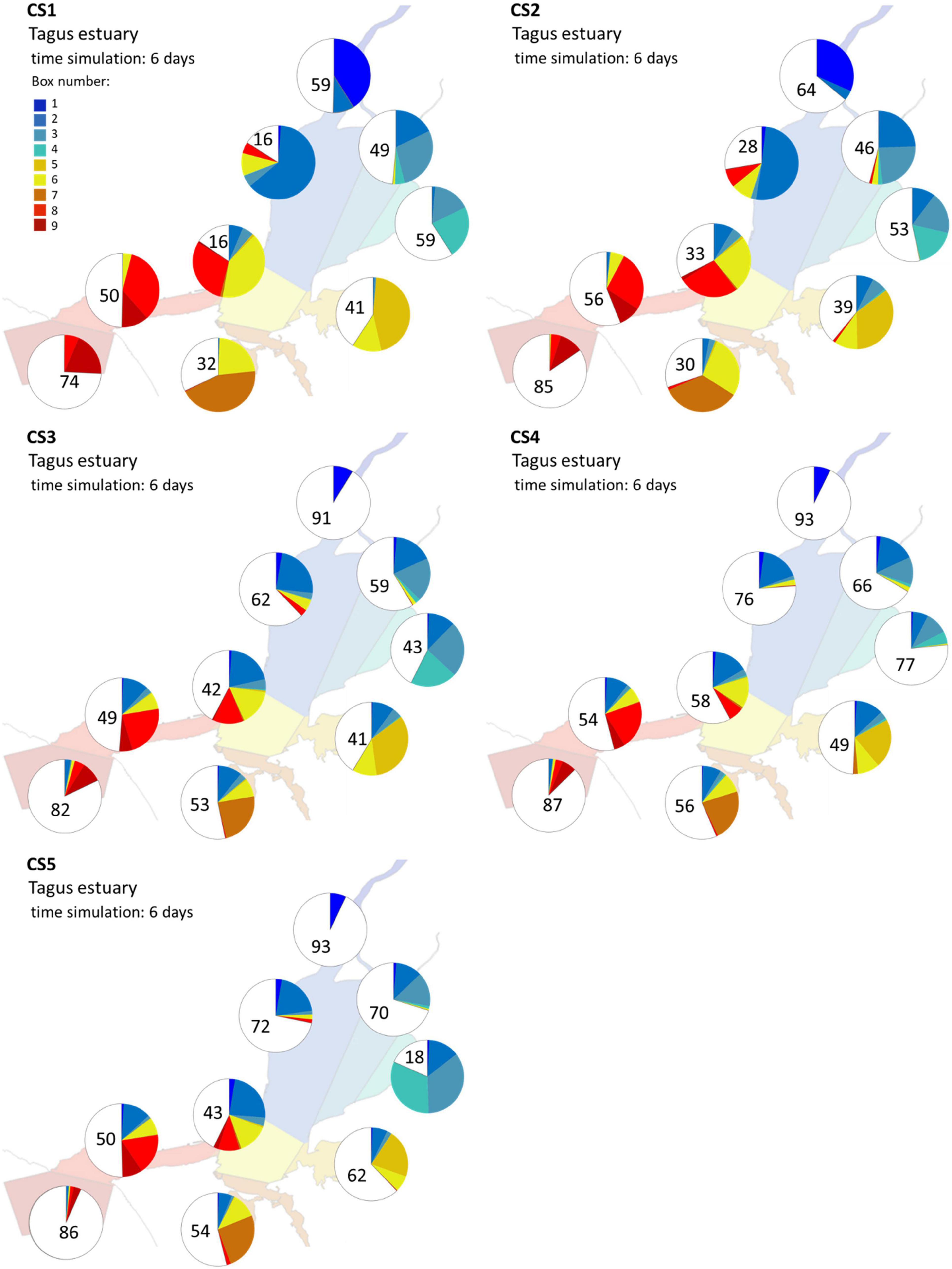
Figure 7. Integrated contribution in each box after 6 days of simulation. White slice corresponds to new water (from river or/and seawater).

Discussion

Nowadays, with the improvement of computational capacity, high-resolution (3D) models, from an eulerian perspective, reproduce with great reliability the hydrodynamics of a system on an appropriate spatial and temporal scale to represent local circulation patterns, conditioned either by complex morphological variations (e.g., jagged coastlines, abrupt changes in bathymetry, etc.), or by sudden variations in the metocean data (e.g., peak discharges, changes in wind intensity and direction, point sewage discharges). This type of 3D implementation becomes relevant in estuaries with complex morphology with important discharges of fresh water, which makes the density currents dominate the water circulation. On the other hand, the relative importance of the wind on the water column varies from the surface toward the bottom, therefore affecting the residual transport (velocity currents). From a Lagrangian point of view, the capacity of computing a high number of tracers increases the degree of confidence, since a better statistical representation of the tracers’ dispersion is achieved (Wagner et al., 2019).

Although the eulerian method considers the effects of advection and diffusion—as opposed to the Lagrangian method applied in this study—when the aim is to describe the movement of tracers, the Lagrangian method should be applied. Indeed, this method simulates the heterogeneity of water exchange in different areas of the estuary and describes the pathways of the tracers (in this work the lagrangian model implementation behaves as a particle-tracking model). Particle-tracking models can provide accurate, detailed spatiotemporal information on the trajectory of tracers, and dispersion history, as they can easily tag tracers with a common origin. The particles were treated as passive drifters, exclusively driven by circulation and diffusion. This allows the identification of water masses (boxes) and to relate tracers’ position at any instant of time with their initial point of release. However, this type of models present some limitations, as precise renewal time is difficult to define. Indeed, by definition, both RT and ET are achieved when all the water in the estuary is completely renewed. This will lead to unrealistic values of these hydrodynamic indicators. To overcome this issue, RT and ET can be considered achieved at the time when a determined residual amount of water remains in the water body (Braunschweig et al., 2003; Xu and You, 2017). In the present study it was assumed that RT is reached when 80% of the tracers has left the box for the first time and ET is reached when the number of tracers in a box never exceeded 20% (after dropping below this number). This interpretation of residual water was based on the analysis of the tracers released in the estuary and in each box for the case study with a medium river discharge (CS2), the most usual of the Tagus River. Indeed, and generally speaking, the exponential function changed its slope when approximately 20% of the tracers were within the estuary or within the boxes where they were released. This was verified for the estuary as a whole and for all individual boxes. This threshold was also adopted by Braunschweig et al. (2002) for the same study area of the present research.

Both RT and ET are affected by the choice of the initial time to start the simulations (tide period), but mainly for high river discharges, since most of the tracers tend to leave the estuary rapidly. For this reason, all the simulations performed started during the low tide (ebb filling), as this prevented the tracers from leaving the estuary right after they were released. From a management point of view this is the most unfavorable situation.

In this study, it was observed that with the increase of the river discharge the currents generated increased in velocity, leading to an increasing rate of the Lagrangian tracers that left the estuary, which was reflected in both RT and ET determined, that passed from 59 to 3.5 days for the whole estuary. Under summer conditions, when the river discharge is low and the wind intensity is weak (CS1), the values of RT and ET were the highest achieved. During the summer, these indicators were mainly influenced by the tide and the effects of neap and spring tides were clearly visible. Indeed, during neap tides the water was retained longer in the estuary, whereas, during spring tides, the water was flushed faster from the water body. For CS2, in addition to the importance of the tide, the current intensity within the estuary increased in significance due to the increase of the river discharge, which led to the decrease of both RT and ET. In the case of high and extreme river discharges (CS3 to 5), even though the wind direction promoted the retention of the tracers, the high current velocities generated by the river discharge counteracted this effect, causing tracers to be quickly flushed away from the estuary to the sea, which justifies the low RT and ET values obtained. Indeed, although the Tagus estuary is tide-dominated rather than river-dominated, the influence of the river discharge in the estuary water dynamics became more significant when the mean river discharge was higher than 1,231 m³/s. In this case, the renewal of the estuary’s water occurred very quickly (less than 1 week), which was reflected in the values of both RT and ET, estimated at 5 days for CS3.

Our results showed that for a mean river discharge of 317 m³/s RT was achieved 11 days earlier than the one reported by Braunschweig et al. (2003) who estimated a RT of 25 days for a mean river discharge of 330 m³/s. The difference obtained may be related to the approach used. Indeed, those authors used a constant river discharge and wind during the simulation period, whereas in the present study real (and variable) metocean data were used. Moreover, those authors used a 2D depth-integrated model. One of the advantages in using 3D models, as in the present study, when compared to 2D models, is that 3D models take into consideration the variation of water velocity within the water column, with higher water velocities registered at the surface layers of the water column and lower velocities at the bottom.

From a management point of view, it is more interesting to understand the variation of RT and ET within the estuary over time, and under distinct river discharge scenarios, and how water exchanges in different areas of it, since it allows to identify the most vulnerable areas of the estuary. It also allows to foresee the potential impact of different actions/decisions and input of pollutants on the ecosystem. In general, areas with higher RT and/or ET are the ones that are more vulnerable to the accumulation of contaminants (Sale et al., 2011). To this end, the present work considered 9 different areas.

Under summer conditions, when the river discharge is low, both RT and ET were higher within the main body of the estuary and the bays. However, the exchange of water masses occurred mainly among contiguous areas due to the low current velocity generated by the river discharge, with the exceptions of boxes 6, 8 and 9, which received water from all boxes. With the increase of the river discharge, although the RT and ET decreased in all boxes, the areas located in the south margin presented higher RT and ET than in the remaining estuary. The joint action of the currents created by the tide and the river discharge caused the water in the estuary to mix more, thus increasing the influence of the water masses from one box in the others.

In box 1, which corresponds to the Tagus River area, differences between RT and ET were only observed when the river discharge was low, with these hydrodynamic indicators reaching 1 day for significant river discharges (CS3 to 5). At low and medium mean river discharges, the water in this box was mixed with water from box 2, reflecting the influence of the tide on the most upstream area of the estuary. With higher river discharges, the renewal of the water occurred extremely fast, which explains the inexistence of tracers from other boxes. The dynamics between saltwater and freshwater is of major relevance in estuarine areas since it affects residual velocities, residence times, exposure times, and water quality, being tides and freshwater discharges the main drives of this dynamic (Rodrigues et al., 2019). This dynamic is mainly affected during droughts as during low river discharge periods the saltwater can propagate further upstream. The results obtained in the present study indicate that only at low and mean river discharges (CS1 and 2) occurred the intrusion of the saltwater in the upper Tagus estuary. However, as reported by Rodrigues et al. (2019), salinity intrusion in the upper estuary depends not only on the river flow but also on the duration of the droughts. In Portugal, 2017 was considered a drought year (CS1) and therefore it was registered low rivers discharges during several months (Figure 2) which has favored the increase of the saltwater intrusion in the upper estuary, which may have affected several economic sectors, such as public water supply, and agriculture (Stahl et al., 2016; Rodrigues et al., 2019).

The main differences observed for the first four case studies were mainly observed in both the main body of the estuary and in the bays (boxes 2 to 7). The CS1 (low mean river discharge in the summer) presented the highest ET values, which reflects the low water velocities registered within the estuary. This indicates that the tide was the main driver of tracer dispersion. In this CS and for boxes 2 to 7, the ET ranged between 16 and 59 days, with the highest values registered in boxes 2 and 3, both located in the main body of the estuary. Since these two boxes cover a significant area of the estuary in its main flow direction, under low river discharges the harmonic effect of the tide caused tracers to return to those boxes for an extended period. This harmonic effect of the tide became less evident with the increase of the river discharge since the current velocities within the estuary increased, which explains the decrease of ET values determined for boxes 2 to 7 in the CS2, 3, and 4. It is interesting to note that with the increase of the river discharge the ET in the main body of the estuary tended to decrease to 1 to 2 days and to match RT, indicating that the tracers left the estuary very quickly, whereas in the bays, higher ETs were determined even in periods of extreme river discharge (CS4; 5 and 6 days for boxes 5 and 7, respectively). Thus, in the bays the tracers returned several times to these areas before leaving the estuary which explains the high differences observed between RT and ET in these areas. This is related to the lower current velocities registered, morphology, and the water recirculation pattern observed in this part of the estuary, which promoted the retention of the tracers in those areas for a longer time. Moreover, for all river discharges, results showed that the bays received little water from the most downstream areas (boxes 8 and 9) which is related to the circulation patterns observed in the estuary that prevented water from those areas to enter the bays, especially during the tidal flood.

It is also important to highlight, that boxes 3 and 4 did not receive tracers from boxes located downstream regardless the river discharge, suggesting that the Tagus and Sorraia river discharges were the principal mechanism contributing to the water renewal in these boxes. Although these boxes are also located in the main body of estuary, a great part of their area is comprised of intertidal zones which favored the quick exit of tracers released in these boxes, to other boxes during the ebb tide, mainly the ones located downstream. However, tracers tended to return to these boxes during the flood tide which explains the differences observed between RT and ET in CS1. For medium to extreme river discharges this difference disappeared in box 3, whereas in box 4 this was only registered for extreme river discharges.

The CS5 concerns to an extreme event that led to a mean river discharge of 6,333 m³/s with a maximum Tagus River discharge of 9,874 m³/s, one of the highest discharges registered in the last 100 years. In this event, the river discharge remained extremely high for over two consecutive days (mean river discharge of 8,429 m³/s). Since these discharges are so unusual, this case study is analyzed separately. It was observed that both RT and ET increased in 1 day for the whole estuary, relatively to the other extreme event studied (CS4), suggesting that the hydrodynamics of the estuary suffered changes, mainly in the south part of the main body, and in the bays. Indeed, during this event a huge current was generated in the principal flow channels which split the estuary into two zones with consequences on both RT and ET determined for the different boxes. The current velocity was so high that in the north part of the estuary (boxes 1, 2, 6, 8, and 9), tracers were rapidly flushed away from the estuary, producing equal values of RT and ET for this area in CS4. The main difference observed was related to the south part of the estuary (boxes 3, 4, 5, and 7), where both RT and ET increased comparatively to CS4. The high current velocities in the main flow channel created a transport barrier that impeded tracers from leaving their boxes of origin, and that pushed tracers released in these boxes toward the south margin of the estuary or into the bays. The retention of the tracers in this part of the estuary was significant enough to justify the increase in both RT and ET for the whole estuary, from 3.5 in CS4 to 4.5 in the CS5. This also justifies the results obtained for those areas when the integrated water fraction was analyzed.

The results achieved in the present study allowed to identify the most vulnerable areas within the estuary, based on the integrated analysis of ET values determined for each box and water exchange between boxes. For management purposes it is better to consider ET than RT. Indeed, while RT only accounts for the time a particle stays in a given area until it exits that area for the first time, ET accounts for the total time spent within the area of interest (Monsen et al., 2002), i.e., it considers all subsequent re-entries (de Brauwere et al., 2011). Thus, ET is of particular relevance in systems with oscillatory tidal flows, as it is the case of the Tagus estuary, since quantifies the exposure time of a system, or an area of it, to a specific contaminant. The vulnerability of the areas is intrinsically dependent on the river discharge. Indeed, under summer conditions when the river discharge was low, all the main body of the estuary can be considered vulnerable due to the high ETs observed. However, when the river discharge increased, the ET determined decreased significantly in the north part of the main body and therefore the most vulnerable areas are all located in its south margin and mainly in the bays. Considering only the medium and high river discharges, attention should also be paid to boxes 2 and 6, as these boxes contributed with a significant amount of water in the bays. Notwithstanding, based on the position of the main flow channels and the circulation patterns observed within the estuary, it is believed that the water that entered the bays from box 6 came from a small area of it, mainly from the area located near or south of the main flow channels of the estuary. This can be inferred by tracking over time and at different tidal levels the position of the tracers that were released in this box. Fonseca et al. (2020) conducted a study in the Tagus estuary to characterize the transport pathways of pharmaceuticals released from wastewater outfalls and found the same vulnerable areas identified in the present study. These authors found that the south margin of the estuary as well as the bays are the areas within the estuary that are more prone to environmental degradation due to increased exposure to pharmaceuticals, regardless the river discharge.

It is known that the vulnerability of a given area in a water body is also extremely dependent on the type of particles to be studied. Indeed, it must be taken into account that this study is more significant for conservative particles like some nanoparticles or plastics where its motion is only due to the bulk motion of water. However, for particles that lose their “identity” of origin (e.g., nutrients or compounds that vary with the biogeochemical conditions of the receptor medium over time), the results should be analyzed cautiously. In this case, and although the proposed methodology can be applied, processes (degradation, biogeochemical processes among others) must be associated to the particles in order to reproduce their dilution or concentration within the system. Nevertheless, Sale et al. (2011) suggested that it is in areas with longer residence times where the potential for heat, plankton, and dissolved substances are more likely to accumulate. The probability of proliferation of organisms will be higher in these areas, especially in times of high temperatures and with a significant input of nutrients. These areas are also the most prone to the deposition of dissolved particles, which may affect benthic communities (Sale et al., 2011). Boyer et al. (1997), observed spatial differences in total organic nitrogen, total phosphorus, and phytoplankton biomass (as well as salinity and total organic carbon) in Florida Bay’s due to differences in freshwater inputs and water residence time. Sharpley et al. (2013), reported “hotspots” of phosphorus retention and cycling in areas with slower flows and longer water retention times as well as in areas with sharp gradients in water and sediment retention times. Duarte et al. (2001) using a 2D-hydrodynamic model for the Mondego estuary in order to determine the residence times variability and to assess their effect on the estuarine eutrophication vulnerability and found that eutrophication is more likely to occur in its south arm due to the high residence times observed.

The Water Framework Directive (WFD-EU) considers water quality in its broadest and “ecological” sense and requires the assessment of a wide range of biological, hydromorphological and physico-chemical quality elements to determine the water quality status of the transitional water bodies. Water residence time is one of the hydromorphological quality elements that can be used in this assessment (Monsen et al., 2002; Sincock et al., 2003). Since the main water masses defined for the Tagus estuary in the WFD integrate the monitoring boxes used in the present study, the results of the present research are also an important contribution for the implementation of this European Directive in the TagusROFI.

The present study can be an important tool for decision makers, as it allows making more informed decisions and identifying the potential impacts that these decisions may have on the receiving water body, and how to mitigate them. The Tagus estuary is a highly populated region showing a growing population trend. Therefore an increase of the human pressure over the estuary is expected. For instance, more sewages will need to be built in the near future. Almost all of the present sewages that are located in the municipalities surrounding the Tagus estuary discharge the water directly into the estuary. Where to install new waste water treatment plants and where outfalls should be placed (or relocated), should take into consideration the ET and water exchange among areas of the estuary, in order to avoid the retention of large amounts of nutrients in the estuary for long periods of time, to promote their quick flush to the sea, and to improve the microbiological quality of the Tagus estuarine water. Bacterial contamination is a prevalent problem in the Tagus estuary that contaminates shellfish and affects an important harvesting bivalve activity (Moura et al., 2017, 2018), which occurs prevalently in its main body. Recently, bivalve harvesting was forbidden in one of the most important bivalve fishing areas of the Tagus estuary due to the high levels of contamination of bivalves by Escherichia coli which is causing significant local socio-economic issues. It is believed that one of the main sources of this contamination is probably related to the inadequate treatment of the sewage water released into the estuary. The results obtained in the present study can be useful to support decisions on how this issue can be overcome, since it gives important insights, for instance, on the areas to where waters from sewage systems should be released in order to promote its rapid exit from the estuary or to minimize the bacterial contamination of the most important bivalve beds. This is just an example on how ET and water exchange within the estuary can be used in the management of this water body. On the other hand, the methodology used in this work could be useful to predict how the construction of new engineering-building structures within the estuary (such as commercial ports, marinas and dikes) may change water circulation in those areas and how this may affect ET and water exchange nearby.

Conclusion

The 3D version of the MOHID hydrodynamic model coupled to a particle-tracking model (lagrangian tool) was used to assess the effect of five different Tagus River discharge scenarios, ranging from low to extreme, on residence time (RT), exposure time (ET) and integrated water fractions inside pre-established Tagus estuary areas. Particle-tracking models can provide accurate, detailed spatiotemporal information on the trajectory of tracers, and dispersion history, as they can easily tag tracers with a common origin. In this type of models particles are treated as passive drifters, exclusively driven by circulation and diffusion. The increase of the river discharge generated high current velocities which led to a decrease of both RT and ET, from 59 to 3.5 days under a low and extreme river discharge scenario, respectively. Under a low river discharge, significant differences were observed between RT and ET in the areas located in the main body of the estuary and in the bays. As the river discharge increased, RT and ET decreased in all areas of the estuary and those differences tended to disappear. The approach followed, allowed to identify the most vulnerable areas within the estuary, based on the integrated analysis of ET values determined for each box, and water exchange between boxes. It was observed that vulnerability of the areas is related to the river discharge. Under low river discharges, all the main body of the estuary can be considered vulnerable, whereas when the river discharge increases, the most vulnerable areas are all located in its south margin and in the bays. For medium and high river discharges, attention should also be paid to boxes 2 and 6 (located in the central body), as these areas contributed with a significant amount of water to the bays. The present study can be an important tool for decision makers, as it allows making more informed decisions, and is a useful tool to evaluate how management decisions taken in one area may affect other areas. Although the Lagrangian model used behaved as a particle-tracking model, this tool can also be used for non-conservative particles where their properties are taken into consideration, since their physical, chemical, and/or biological properties may vary along the particles trajectory.

Data Availability Statement

The raw data supporting the conclusions of this article will be made available by the authors, without undue reservation.

Author Contributions

HP and RN designed the study. HP ran the model and analyzed the results. HP, JS, and MG interpreted and discussed the results and wrote the first draft of the manuscript. JS helped in the eulerian simulations performed. DG-P designed and programmed the Lagrangian tool. CF made the scripts for the figures. All authors reviewed and made a substantial, direct, and intellectual contribution to the work, and approved the submitted version.

Funding

The present work was supported by FCT/MCTES (PIDDAC) through the project LARSyS–FCT Pluriannual funding 2020–2023 (UIDB/50009/2020) and performed within the framework of the research project “Tackling Marine Litter in the Atlantic Area (CleanAtlantic).” INTERREG Atlantic Area, European Union, European Regional Development Fund (ERDF).

Conflict of Interest

The authors declare that the research was conducted in the absence of any commercial or financial relationships that could be construed as a potential conflict of interest.

Publisher’s Note

All claims expressed in this article are solely those of the authors and do not necessarily represent those of their affiliated organizations, or those of the publisher, the editors and the reviewers. Any product that may be evaluated in this article, or claim that may be made by its manufacturer, is not guaranteed or endorsed by the publisher.

Acknowledgments

The authors would like to acknowledge to Javier Bárcena, research in IH Cantabria, for exchanging ideas, for his kindness and availability, as well as for his contribution to the knowledge acquired. The authors would also like to acknowledge Alejandro Souza (Associate Editor of Frontiers in Marine Science) and two reviewers for valuable comments and suggestions that greatly improved the revised manuscript.

References

APA, (Agência Portuguesa do Ambiente) (2015). Plano de Gestão da Região Hidrográfica do Tejo e Ribeiras do Oeste (RH5), Parte 2—Caracterização e Diagnóstico. Lisboa: Agência Portuguesa do Ambiente, 176.

Google Scholar

Azhikodan, G., and Yokoyama, K. (2016). Spatio-temporal variability of phytoplankton (Chlorophyll-a) in relation to salinity, suspended sediment concentration, and light intensity in a macrotidal estuary. Cont. Shelf Res. 126, 15–26. doi: 10.1016/j.csr.2016.07.006

CrossRef Full Text | Google Scholar

Bárcena, J. F., Claramunt, I., García-Alba, J., Pérez, M. L., and García, A. (2017a). A method to assess the evolution and recovery of heavy metal pollution in estuarine sediments: past history, present situation and future perspectives. Mar. Pollut. Bull. 124, 421–434. doi: 10.1016/j.marpolbul.2017.07.070

PubMed Abstract | CrossRef Full Text | Google Scholar

Bárcena, J. F., García, A., Gómez, A. G., Álvarez, C., Juanes, J. A., and Revilla, J. A. (2012). Spatial and temporal flushing time approach in estuaries influenced by river and tide. An application in Suances Estuary (Northern Spain). Estuar. Coast. Shelf Sci. 112, 40–51. doi: 10.1016/j.ecss.2011.08.013

CrossRef Full Text | Google Scholar

Bárcena, J. F., García-Alba, J., García, A., and Álvarez, C. (2016). Analysis of stratification patterns in river-influenced mesotidal and macrotidal estuaries using 3D hydrodynamic modelling and K-means clustering. Estuar. Coast. Shelf Sci. 181, 1–13. doi: 10.1016/j.ecss.2016.08.005

CrossRef Full Text | Google Scholar

Bárcena, J. F., Gómez, A. G., García, A., Álvarez, C., and Juanes, J. A. (2017b). Quantifying and mapping the vulnerability of estuaries to point-source pollution using a multi-metric assessment: the Estuarine Vulnerability Index (EVI). Ecol. Indic. 76, 159–169. doi: 10.1016/j.ecolind.2017.01.015

CrossRef Full Text | Google Scholar

Bolin, B., and Rodhe, H. (1973). A note on the concepts of age distribution and transit time in natural reservoirs. Tellus 25, 58–62. doi: 10.1111/j.2153-3490.1973.tb01594.x

CrossRef Full Text | Google Scholar

Boyer, J. N., Fourqurean, J. W., and Jones, R. D. (1997). Spatial characterization of water quality in Florida Bay and Whitewater Bay by multivariate analyses: zones of similar influence. Estuaries 20, 743–758. doi: 10.2307/1352248

CrossRef Full Text | Google Scholar

Braunschweig, F., Chambel, P., Martins, F., and Neves, R. (2002). “A methodology to estimate the residence time of estuaries,” in Proceedings of the 11th International conference bienial on Physics of Estuaries and Coastal Seas, PECS 2002. (Hamburgo), 49–52.

Google Scholar

Braunschweig, F., Chambel, P., Martins, F., and Neves, R. (2003). A methodology to estimate the residence time of estuaries. Ocean Dyn. 53, 137–145.

Google Scholar

Bricelj, V. M., and Lonsdale, D. J. (1997). Aureococcus anophagefferens: causes and ecological consequences of brown tides in U.S. mid-Atlantic coastal waters. Limnol. Oceanogr. 42, 1023–1038. doi: 10.4319/lo.1997.42.5_part_2.1023

CrossRef Full Text | Google Scholar

Bricker, S. (1999). National Estuarine Eutrophication Assessment: Effects of Nutrient Enrichment in the Nation’Estuaries. Washington, DC: NOAA.

Google Scholar

Campuzano, F., Brito, D., Juliano, M., Fernandes, R., de Pablo, H., and Neves, R. (2016). Coupling watersheds, estuaries and regional ocean through numerical modelling for Western Iberia: a novel methodology. Ocean Dyn. 66, 1745–1756. doi: 10.1007/s10236-016-1005-4

CrossRef Full Text | Google Scholar

Cavalcante, G. H., Kjerfve, B., and Feary, D. A. (2012). Examination of residence time and its relevance to water quality within a coastal mega-structure: the Palm Jumeirah Lagoon. J. Hydrol. 46, 111–119. doi: 10.1016/j.jhydrol.2012.08.027

CrossRef Full Text | Google Scholar

Cloern, J. E., Jassby, A. D., Schraga, T. S., Nejad, E., and Martin, C. (2017). Ecosystem variability along the estuarine salinity gradient: examples from long-term study of San Francisco Bay. Limnol. Oceanogr. 62, S272–S291. doi: 10.1002/lno.10537

CrossRef Full Text | Google Scholar

de Brauwere, A., de Brye, B., Blaise, S., and Deleersnijder, E. (2011). Residence time, exposure time and connectivity in the Scheldt Estuary. J. Mar. Syst. 84, 85–95. doi: 10.1016/j.jmarsys.2010.10.001

CrossRef Full Text | Google Scholar

de Pablo, H., Sobrinho, J., Garcia, M., Campuzano, F., Juliano, M., and Neves, R. (2019). Validation of the 3D-MOHID hydrodynamic model for the Tagus coastal area. Water (Switzerland) 11:1713. doi: 10.3390/w11081713

CrossRef Full Text | Google Scholar

Defne, Z., and Ganju, N. K. (2015). Quantifying the residence time and flushing characteristics of a shallow, back-barrier estuary: application of hydrodynamic and particle tracking models. Estua. Coast. 38, 1719–1734. doi: 10.1007/s12237-014-9885-3

CrossRef Full Text | Google Scholar

Delesalle, B., and Sournia, A. (1992). Residence time of water and phytoplankton biomass in coral reef lagoons. Cont. Shelf Res. 12, 939–949. doi: 10.1016/0278-4343(92)90053-M

CrossRef Full Text | Google Scholar

Delhez, ÉJ. M., Heemink, A. W., and Deleersnijder, É (2004). Residence time in a semi-enclosed domain from the solution of an adjoint problem. Estuar. Coast. Shelf Sci. 61, 691–702. doi: 10.1016/j.ecss.2004.07.013

CrossRef Full Text | Google Scholar

Dippner, J. W., Bartl, I., Chrysagi, E., Holtermann, P., and Kremp, A. (2019). Lagrangian residence time in the Bay of Gda nsk, Baltic Sea. Front. Mar. Sci 6:725. doi: 10.3389/fmars.2019.00725

CrossRef Full Text | Google Scholar

Duarte, A. A. L. S., Pinho, J. L. S., Pardal, M. A. C., Vieira, J. M. P., and Santos, F. S. (2001). Effect of residence times on river Mondego estuary eutrophication vulnerability. Water Pollut. Res. 44, 329–336. doi: 10.2166/wst.2001.0786

CrossRef Full Text | Google Scholar

Duarte, A. S., Pinho, J., Pardal, M. Â, Neto, J. M., Vieira, J., and Santos, F. S. (2002). “Hydrodynamic modelling for Mondego estuary water quality management,” in Aquatic Ecology of the Mondego River Basin Global Importance of Local Experience, ed. P. M. Graça (Coimbra: Imprensa da Universidade de Coimbra), 29–42. doi: 10.14195/978-989-26-0336-0_3

CrossRef Full Text | Google Scholar

Flather, R. A. (1976). A tidal model of the north-west European continental shelf. Mem. Soc. R. Sci. Liege, Ser. 10, 141–164.

Google Scholar

Fonseca, V. F., Reis-Santos, P., Duarte, B., Cabral, H. N., Caçador, M. I., Vaz, N., et al. (2020). Roving pharmacies: modelling the dispersion of pharmaceutical contamination in estuaries. Ecol. Indic. 115:106437. doi: 10.1016/j.ecolind.2020.106437

CrossRef Full Text | Google Scholar

Fortunato, A. B., Baptista, A. M., and Luettich, R. A. (1997). A three-dimensional model of tidal currents in the mouth of the Tagus estuary. Cont. Shelf Res. 17, 1689–1714. doi: 10.1016/S0278-4343(97)00047-2

CrossRef Full Text | Google Scholar

Fortunato, A. B., Freire, P., Bertin, X., Rodrigues, M., Ferreira, J., and Liberato, M. L. R. (2017). A numerical study of the February 15, 1941 storm in the Tagus estuary. Cont. Shelf Res. 144, 50–64. doi: 10.1016/j.csr.2017.06.023

CrossRef Full Text | Google Scholar

Franz, G., Pinto, L., Ascione, I., Mateus, M., Fernandes, R., Leitão, P., et al. (2014). Modelling of cohesive sediment dynamics in tidal estuarine systems: case study of Tagus estuary, Portugal. Estuar. Coast. Shelf Sci. 151, 34–44. doi: 10.1016/j.ecss.2014.09.017

CrossRef Full Text | Google Scholar

Gameiro, C., Cartaxana, P., and Brotas, V. (2007). Environmental drivers of phytoplankton distribution and composition in Tagus Estuary, Portugal. Estuar. Coast. Shelf Sci. 75, 21–34. doi: 10.1016/j.ecss.2007.05.014

CrossRef Full Text | Google Scholar

Gómez, A. G., Bárcena, J. F., Juanes, J. A., Ondiviela, B., and Sámano, M. L. (2014). Transport time scales as physical descriptors to characterize heavily modified water bodies near ports in coastal zones. J. Environ. Manage. 136, 76–84. doi: 10.1016/j.jenvman.2014.01.042

PubMed Abstract | CrossRef Full Text | Google Scholar

Guerreiro, M., Fortunato, A. B., Freire, P., Rilo, A., Taborda, R., Freitas, M. C., et al. (2015). Evolution of the hydrodynamics of the Tagus estuary (Portugal) in the 21st century. Rev. Gestão Costeira Integrada 15, 65–80. doi: 10.5894/rgci515

CrossRef Full Text | Google Scholar

Huang, W., Liu, X., Chen, X., and Flannery, M. S. (2011). Critical flow for water management in a shallow tidal river based on estuarine residence time. Water Resour. Manag. 25, 2367–2385. doi: 10.1007/s11269-011-9813-2

CrossRef Full Text | Google Scholar

Jambeck, J. R., Geyer, R., Wilcox, C., Siegler, T. R., Perryman, M., Andrady, A., et al. (2015). Plastic waste inputs from land into the ocean. Science 347, 768–771. doi: 10.1126/science.1260352

PubMed Abstract | CrossRef Full Text | Google Scholar

Jay, D. A., Uncles, R. J., Largier, J., Geyer, W. R., Vallino, J., and Boynton, W. R. (1997). A review of recent developments in estuarine scalar flux estimation. Estuaries 20, 262–280. doi: 10.2307/1352342

CrossRef Full Text | Google Scholar

Kako, S., Isobe, A., Kataoka, T., and Hinata, H. (2014). A decadal prediction of the quantity of plastic marine debris littered on beaches of the East Asian marginal seas. Mar. Pollut. Bull. 81, 174–184. doi: 10.1016/j.marpolbul.2014.01.057

PubMed Abstract | CrossRef Full Text | Google Scholar

Kooi, M., Besseling, E., Kroeze, C., Van Wezel, A. P., and Koelmans, A. A. (2018). “Modeling the fate and transport of plastic debris in freshwaters: review and guidance,” in Handbook of Environmental Chemistry, eds M. Wagner and S. Lambert (Cham: Springer), 125–152. doi: 10.1007/978-3-319-61615-5_7

CrossRef Full Text | Google Scholar

Lucas, L. V., and Deleersnijder, E. (2020). Timescale methods for simplifying, understanding and modeling biophysical and water quality processes in coastal aquatic ecosystems: a review. Water 12:2717. doi: 10.3390/w12102717

CrossRef Full Text | Google Scholar

Matso, K. (2018). Flushing Time Versus Residence Time for the Great Bay Estuary. Durham, NH: University of New Hampshire.

Google Scholar

Monsen, N. E., Cloern, J. E., Lucas, L. V., and Monismith, S. G. (2002). A comment on the use of flushing time, residence time, and age as transport time scales. Limnol. Oceanogr. 47, 1545–1553. doi: 10.4319/lo.2002.47.5.1545

CrossRef Full Text | Google Scholar

Moura, P., Garaulet, L. L., Vasconcelos, P., Chainho, P., Costa, J. L., and Gaspar, M. B. (2017). Age and growth of a highly successful invasive species: the manila clam ruditapes philippinarum (adams & reeve, 1850) in the Tagus estuary (Portugal). Aquat. Invasions 12, 133–146. doi: 10.3391/ai.2017.12.2.02

CrossRef Full Text | Google Scholar

Moura, P., Vasconcelos, P., Pereira, F., Chainho, P., Costa, J. L., and Gaspar, M. B. (2018). Reproductive cycle of the Manila clam (Ruditapes philippinarum): an intensively harvested invasive species in the Tagus Estuary (Portugal). J. Mar. Biol. Assoc. United Kingdom 98, 1645–1657. doi: 10.1017/S0025315417001382

CrossRef Full Text | Google Scholar

Neves, F. (2010). Dynamics and Hydrology of the Tagus Estuary: Results From in Situ Observations Ph.D. thesis. Available online at: http://repositorio.ul.pt/handle/10451/2003 (accessed February 25, 2021).

Google Scholar

Ohman, M. D., and Wood, S. N. (1996). Mortality estimation for planktonic copepods: Pseudocalanus newmani in a temperate fjord. Limnol. Oceanogr. 41, 126–135. doi: 10.4319/lo.1996.41.1.0126

CrossRef Full Text | Google Scholar

Oliveira, A., and Baptista, A. M. (1997). Diagnostic modeling of residence times in estuaries. Water Resour. Res. 33, 1935–1946. doi: 10.1029/97WR00653

CrossRef Full Text | Google Scholar

Portela, L. I., and Neves, R. (1994). Numerical modelling of suspended sediment transport in tidal estuaries: a comparison between the Tagus (Portugal) and the Scheldt (Belgium-the Netherlands). Netherlands J. Aquat. Ecol. 28, 329–335. doi: 10.1007/bf02334201

CrossRef Full Text | Google Scholar

Raimonet, M., and Cloern, J. E. (2017). Estuary–ocean connectivity: fast physics, slow biology. Glob. Chang. Biol. 23, 2345–2357. doi: 10.1111/gcb.13546

PubMed Abstract | CrossRef Full Text | Google Scholar

Rodrigues, M., Fortunato, A. B., and Freire, P. (2019). Saltwater intrusion in the upper tagus estuary during droughts. Geosciences 9:400. doi: 10.3390/geosciences9090400

CrossRef Full Text | Google Scholar

Rusu, L., Bernardino, M., and Guedes Soares, C. (2011). Modelling the influence of currents on wave propagation at the entrance of the Tagus estuary. Ocean Eng. 38, 1174–1183. doi: 10.1016/j.oceaneng.2011.05.016

CrossRef Full Text | Google Scholar

Sale, P. F., Feary, D. A., Burt, J. A., Bauman, A. G., Cavalcante, G. H., Drouillard, K. G., et al. (2011). The growing need for sustainable ecological management of marine communities of the Persian Gulf. Ambio 40, 4–17. doi: 10.1007/s13280-010-0092-6

PubMed Abstract | CrossRef Full Text | Google Scholar

Sharpley, A., Jarvie, H. P., Buda, A., May, L., Spears, B., and Kleinman, P. (2013). Phosphorus legacy: overcoming the effects of past management practices to mitigate future water quality impairment. J. Environ. Qual. 42, 1308–1326. doi: 10.2134/jeq2013.03.0098

PubMed Abstract | CrossRef Full Text | Google Scholar

Signell, R. P., Jenter, H. L., and Blumberg, A. F. (2000). Predicting the physical effects of relocating Boston’s sewage outfall. Estuar. Coast. Shelf Sci. 50, 59–71. doi: 10.1006/ecss.1999.0532

CrossRef Full Text | Google Scholar

Sincock, A. M., Wheater, H. S., and Whitehead, P. G. (2003). Calibration and sensitivity analysis of a river water quality model under unsteady flow conditions. J. Hydrol. 277, 214–229. doi: 10.1016/S0022-1694(03)00127-6

CrossRef Full Text | Google Scholar

Sobrinho, J., de Pablo, H., Pinto, L., and Neves, R. (2021). Improving 3D-MOHID water model with an upscaling algorithm. Environ. Modell. Softw. 135:104920. doi: 10.1016/j.envsoft.2020.104920

CrossRef Full Text | Google Scholar

Spaulding, M. L. (2017). State of the art review and future directions in oil spill modeling. Mar. Pollut. Bull. 115, 7–19. doi: 10.1016/j.marpolbul.2017.01.001

PubMed Abstract | CrossRef Full Text | Google Scholar

Stahl, K., Kohn, I., Blauhut, V., Urquijo, J., Stefano, L. D., Acácio, V., et al. (2016). Impacts of European drought events: insights from an international database of text-based reports. Nat. Hazards Earth Syst. Sci. 16, 801–819. doi: 10.5194/nhess-16-801-2016

CrossRef Full Text | Google Scholar

Sun, J., Lin, B., Li, K., and Jiang, G. (2014). A modelling study of residence time and exposure time in the Pearl River Estuary, China. J. Hydro Environ. Res. 8, 281–291. doi: 10.1016/j.jher.2013.06.003

CrossRef Full Text | Google Scholar

Takeoka, H. (1984). Fundamental concepts of exchange and transport time scales in a coastal sea. Cont. Shelf Res. 3, 311–326. doi: 10.1016/0278-4343(84)90014-1

CrossRef Full Text | Google Scholar

Tapia González, F. U., Herrera-Silveira, J. A., and Aguirre-Macedo, M. L. (2008). Water quality variability and eutrophic trends in karstic tropical coastal lagoons of the Yucatán Peninsula. Estuar. Coast. Shelf Sci. 76, 418–430. doi: 10.1016/j.ecss.2007.07.025

CrossRef Full Text | Google Scholar

Trancoso, A. R. (2012). Operational Modelling as a Tool in Wind Power Forecasts and Meteorological Warnings Master thesis. Available online at: https://www.researchgate.net/publication/285097114_Operational_modelling_ as_a_tool_in_wind_power_forecasts_and_meteorological_warnings (accessed January 6, 2021).

Google Scholar

Valente, A. S., and da Silva, J. C. B. (2009). On the observability of the fortnightly cycle of the Tagus estuary turbid plume using MODIS ocean colour images. J. Mar. Syst. 75, 131–137. doi: 10.1016/j.jmarsys.2008.08.008

CrossRef Full Text | Google Scholar

Valiela, I., McClelland, J., Hauxwell, J., Behr, P. J., Hersh, D., and Foreman, K. (1997). Macroalgal blooms in shallow estuaries: controls and ecophysiological and ecosystem consequences. Limnol. Oceanogr. 42, 1105–1118. doi: 10.4319/lo.1997.42.5_part_2.1105

PubMed Abstract | CrossRef Full Text | Google Scholar

Vargas, C., Oliveira, F., Oliveira, A., and Charneca, N. (2008). Flood Vulnerability analysis of an estuarine beach: application to Alfeite Sand Spit (Tagus Estuary). Integr. Zool. Manag. J. 8, 25–43.

Google Scholar

Vaz, N., Mateus, M., and Dias, J. M. (2011). Semidiurnal and spring-neap variations in the Tagus Estuary: application of a process-oriented hydro-biogeochemical model. J. Coast. Res. 2011, 1619–1623.

Google Scholar

Wagner, P., Rühs, S., Schwarzkopf, F. U., Koszalka, I. M., and Biastoch, A. (2019). Can Lagrangian tracking simulate tracer spreading in a high-resolution ocean general circulation model? J. Phys. Oceanogr. 49, 1141–1157. doi: 10.1175/JPO-D-18-0152.1

CrossRef Full Text | Google Scholar

Xiong, J., Shen, J., Qin, Q., and Du, J. (2021). Water exchange and its relationships with external forcings and residence time in Chesapeake Bay. J. Mar. Syst. 215:103497. doi: 10.1016/j.jmarsys.2020.103497

CrossRef Full Text | Google Scholar

Xu, T., and You, X. (2017). Lagrangian modeling of particle residence time in the oujiang river estuary, china. Fresenius Environ. Bull. 26, 762–774.

Google Scholar

Yu, X., Shen, J., and Du, J. (2021). An inverse approach to estimate bacterial loading into an estuary by using field observations and residence time. Mar. Environ. Res. 166:105263. doi: 10.1016/j.marenvres.2021.105263

PubMed Abstract | CrossRef Full Text | Google Scholar

Yuan, D., Lin, B., and Falconer, R. A. (2007). A modelling study of residence time in a macro-tidal estuary. Estuar. Coast. Shelf Sci. 71, 401–411. doi: 10.1016/j.ecss.2006.08.023

CrossRef Full Text | Google Scholar

Zhang, W. G., Wilkin, J. L., and Schofield, O. M. E. (2010). Simulation of water age and residence time in New York Bight. J. Phys. Oceanogr. 40, 965–982. doi: 10.1175/2009JPO4249.1

CrossRef Full Text | Google Scholar

Zhang, X., and Wang, P. (2012). “Numerical study of residence time in Daliaohe Estuary,” in Proceedings of the 2012 International Conference on Computer Distributed Control and Intelligent Environmental Monitoring, CDCIEM 2012. (Zhangjiajie), 451–455. doi: 10.1109/CDCIEM.2012.113

CrossRef Full Text | Google Scholar

Zimmerman, J. T. F. (1976). Mixing and flushing of tidal embayments in the western Dutch Wadden Sea part I: distribution of salinity and calculation of mixing time scales. Netherlands J. Sea Res. 10, 149–191. doi: 10.1016/0077-7579(76)90013-2

CrossRef Full Text | Google Scholar