Temperature and Salinity Inverted for a Mediterranean Eddy Captured With Seismic Data, Using a Spatially Iterative Markov Chain Monte Carlo Approach

Xiao, Wuxin; Sheen, Katy Louise; Tang, Qunshu; Shutler, Jamie; Hobbs, Richard; Ehmen, Tobias

doi:10.3389/fmars.2021.734125

ORIGINAL RESEARCH article

Front. Mar. Sci., 20 December 2021

Sec. Ocean Observation

Volume 8 - 2021 | https://doi.org/10.3389/fmars.2021.734125

This article is part of the Research Topic Acoustically Mapping the Ocean View all 10 articles

Temperature and Salinity Inverted for a Mediterranean Eddy Captured With Seismic Data, Using a Spatially Iterative Markov Chain Monte Carlo Approach

$\r\nWuxin Xiao*$ Wuxin Xiao^1*

¹College of Life and Environmental Sciences, University of Exeter, Penryn Campus, Penryn, United Kingdom
²Key Laboratory of Ocean and Marginal Sea Geology, South China Sea Institute of Oceanology, Innovation Academy of South China Sea Ecology and Environmental Engineering, Chinese Academy of Sciences (CAS), Guangzhou, China
³Department of Earth Sciences, Durham University, Durham, United Kingdom

Ocean submesoscale dynamics are thought to play a key role in both the climate system and ocean productivity, however, subsurface observations at these scales remain rare. Seismic oceanography, an established acoustic imaging method, provides a unique tool for capturing oceanic structure throughout the water column with spatial resolutions of tens of meters. A drawback to the seismic method is that temperature and salinity are not measured directly, limiting the quantitative interpretation of imaged features. The Markov Chain Monte Carlo (MCMC) inversion approach has been used to invert for temperature and salinity from seismic data, with spatially quantified uncertainties. However, the requisite prior model used in previous studies relied upon highly continuous acoustic reflection horizons rarely present in real oceanic environments due to instabilities and turbulence. Here we adapt the MCMC inversion approach with an iteratively updated prior model based on hydrographic data, sidestepping the necessity of continuous reflection horizons. Furthermore, uncertainties introduced by the starting model thermohaline fields as well as those from the MCMC inversion itself are accounted for. The impact on uncertainties of varying the resolution of hydrographic data used to produce the inversion starting model is also investigated. The inversion is applied to a mid-depth Mediterranean water eddy (or meddy) captured with seismic imaging in the Gulf of Cadiz in 2007. The meddy boundary exhibits regions of disrupted seismic reflectivity and rapid horizontal changes of temperature and salinity. Inverted temperature and salinity values typically have uncertainties of 0.16°C and 0.055 psu, respectively, and agree well with direct measurements. Uncertainties of inverted results are found to be highly dependent on the resolution of the hydrographic data used to produce the prior model, particularly in regions where background temperature and salinity vary rapidly, such as at the edge of the meddy. This further advancement of inversion techniques to extract temperature and salinity from seismic data will help expand the use of ocean acoustics for understanding the mesoscale to finescale structure of the interior ocean.

Introduction

Mediterranean water eddies, or “meddies,” are anti-cyclonically rotating, sub-surface lenses of warm, salty water formed where the Mediterranean Sea outflows into the Atlantic Ocean (e.g., Richardson et al., 2000). They are thought to separate from the Mediterranean Undercurrent as it interacts with topographic features such as canyons along the Iberian continental margin (Serra et al., 2005). Meddies are typically 20–100 km in diameter, have rotation periods of a few days, and have cores that are 500–1,000 m thick centered near 1,200 m depth (Armi and Zenk, 1984; Prater and Sanford, 1994; Richardson et al., 2000). Meddies carry waters with temperatures of 11.5–13.5°C and salinities 36.2–36.8 within their cores (Armi and Zenk, 1984; Schultz-Tokos and Rossby, 1991; Pingree and Le Cann, 1993; Prater and Sanford, 1994; Richardson et al., 2000; Paillet et al., 2002; Carton et al., 2010). With 15–20 Meddies produced annually, meddies transport most of the Mediterranean outflow into the wider Atlantic Ocean (Bower et al., 1997; Richardson et al., 2000).

While the cores of meddies are largely homogeneous, high gradients of temperature and salinity, with interleaving, thermohaline intrusions and “layering” are commonly found at the meddy periphery (Armi and Zenk, 1984; Ruddick, 1992; Ménesguen et al., 2009; Pinheiro et al., 2010; Biescas et al., 2014). These layering structures typically have vertical scales of 20–75 m and are thought to be generated by both stirring and double diffusive processes (Ruddick and Hebert, 1988; Pinheiro et al., 2010; Song et al., 2011; Meunier et al., 2015). Such finescale layering formations likely play a key role in the eventual disintegration of the meddy through the shedding and mixing of their Mediterranean-water core to the surrounding cooler, fresher Atlantic waters (Armi et al., 1989; Hebert et al., 1990; Song et al., 2011; Hua et al., 2013; Meunier et al., 2015). Meddies are also known to decay through collision with seamounts (Schultz Tokos et al., 1994; Richardson et al., 2000). Accounting for these various mixing and decay processes, meddies typically last 1–5 years. With translation speeds of a few cm/s, typically south-westward, they can transport Mediterranean water more than a thousand kilometers from its source (Richardson et al., 2000).

Seismic oceanography has been used to image the finescale to submesoscale structures associated with meddies, aiding understanding of the important role that they play in the redistribution of heat and salt across the North Atlantic (Wang and Dewar, 2003; Biescas et al., 2008; Ménesguen et al., 2009; Papenberg et al., 2010; McWilliams, 2016). Seismic oceanography is a widely used technique that utilizes acoustic energy (of typically 20–200 Hz) reflected at temperature and salinity changes within the water column (Holbrook et al., 2003; Ruddick et al., 2009; Sallarès et al., 2009). Resultant acoustic images display oceanic structure with vertical and horizontal resolutions of order ten meters, over regions tens of km long and to full depth (e.g., Sheen et al., 2012; Gunn et al., 2020). Physical phenomena such as internal waves, heat fluxes and turbulent mixing can be quantitatively estimated by interpreting the spatial structure of reflectors, which are often assumed to follow isopycnals (Sheen et al., 2009; Papenberg et al., 2010; Fortin et al., 2016, 2017; Sallarès et al., 2016; Dickinson et al., 2017; Gunn et al., 2018, 2020). Seismic ocean data essentially captures the relative strength of the thermohaline stratification but does not explicitly measure absolute values of temperature, salinity or density. As such the ability to interpret and quantitatively assess many of the fascinating structures imaged is limited. Seismic inversion techniques which produce high resolution temperature and salinity fields with quantified uncertainties are required and could represent a step-change in our ability to observe the sub-surface ocean on sufficient spatial scales.

Various different strategies have been applied to solve the ocean seismic inversion problem including both full waveform inversion and the inversion of temperature and salinity from acoustic impedance calculated from reflection amplitudes and hydrographic data (Wood et al., 2008; Papenberg et al., 2010; Kormann et al., 2011; Bornstein et al., 2013; Biescas et al., 2014; Padhi et al., 2015; Dagnino et al., 2016). The accuracy of inverted temperature and salinity values are typically estimated by comparison to “co-located” hydrographic data such as conductivity-temperature-depth (CTD) casts or expendable bathymetry (XBT) data. This approach to estimating the inversion uncertainty, however, does not account for a time or depth shift between CTD/XBT and seismic data. As such Tang et al. (2016) developed a Bayesian Markov Chain Monte Carlo (MCMC) inversion technique. In this Bayesian approach, the uncertainty of inverted temperature and salinity values are assessed by how well a distribution of possible solutions fit the observed seismic acoustic reflectivity. However, due to the band-limited nature of seismic data, which fails to capture the background thermohaline structure (i.e., scales greater than ∼100 m), the MCMC approach only encompasses the uncertainty of the high frequency temperature and salinity variability. The MCMC approach therefore requires an accurate background temperature-salinity starting model to provide information about the larger scale background variability. Tang et al. (2016) found that a starting model produced from available hydrographic (i.e., XBT cast) data did not capture enough of the horizontal variability to successfully recover thermohaline fields using the MCMC approach. However, by applying the MCMC method to the specific case of an internal solitary wave, Tang et al. (2016) were instead able to exploit the highly continuous nature of the internal wave reflection horizons to produce an initial model with sufficient horizontal resolution: the undulating seismic reflection horizons associated with the solitary internal wave were treated as isothermals/isohalines and used to characterize the finer scale horizontal temperature and salinity variability in between XBT casts. However, the internal solitary wave is a rather unique situation: firstly, it is not always possible to assume that reflection horizons follow isothermals or isopycnals (Biescas et al., 2014); secondly, reflection horizons are typically highly discontinuous due to complex water structures, instabilities, or unstable seismic acquisition conditions and noise. To enable the MCMC inversion technique to be applied more ubiquitously across seismic datasets, here a spatially iterative MCMC inversion approach is developed which allows the accurate inversion of temperature and salinity from a prior model built from XBT data alone. The uncertainty associated with the low frequency starting model is assessed and incorporated into final inverted confidence limits, alongside the dependence on the sampling resolution of the input hydrographic data.

This study focuses on seismic oceanographic data collected by the Geophysical Oceanography (GO) research survey in 2007 (Hobbs, 2007). The seismic data are unique as XBT casts were deployed at unusually high spatial resolutions during seismic acquisition (e.g., typically every 2 km). These data are therefore ideal for investigating the influence of prior model resolution on inversion results and providing a comprehensive dataset with which to compare inverted values. Furthermore, the GO survey focused on imaging sub-surface meddies, which typically display rapidly changing temperatures and salinities and disrupted reflectivity at their boundaries (Biescas et al., 2008; Ménesguen et al., 2009). These data thus provide a challenging environment with which to test the inversion.

Materials and Methods

Data Acquisition and Processing

The seismic transect analyzed here, GOLR12, was acquired between 09:37 and 17:45 on the 7th May 2007, in the Gulf of Cadiz (Figure 1). Data were acquired as part of the Geophysical Oceanography (GO) cruise number D318b on the RRS Discovery. The seismic source consisted of six Bolt 1500LL airguns with a usable bandwidth of 5–70 Hz. The source array was shot every 20 s and the acoustic reflection energy was recorded using a 2,400 m long SERCEL streamer with 192 channels and 12.5 m group spacing. Standard signal processing was carried out with particular attention to retaining true reflection amplitudes, paramount for later inversion. Seismic data processing included: (1) Geometry setting; (2) Removal of direct waves using an eigenvector filter applied to the raw shot gathers (Jones and Levy, 1987); (3) Incident angle, directivity and spherical divergence corrections; (4) Noise attenuation by applying a Butterworth band pass filter of 10–80 Hz to shot gathers and compressing traces of anomalous amplitudes; (5) Common midpoint (CMP) sorting; (6) Velocity picking performed every 100 CMPs; (7) Source deconvolution: a reweight deconvolution strategy (Sacchi, 1997) was applied to extract the reflectivity from stacked seismic sections basing on the source wavelet, which was modeled from the source array geometry and airgun volumes using the Nucleus+ software; (8) Amplitude calibration using the seafloor reflection and its first multiple (Warner, 1990); (9) Conversion from two-way travel time to depth using sound velocity derived from XBT data. The final stacked section is shown in Figure 2A. The same seismic line (GOLR12) is used to invert the temperature and salinity by Papenberg et al. (2010).

FIGURE 1

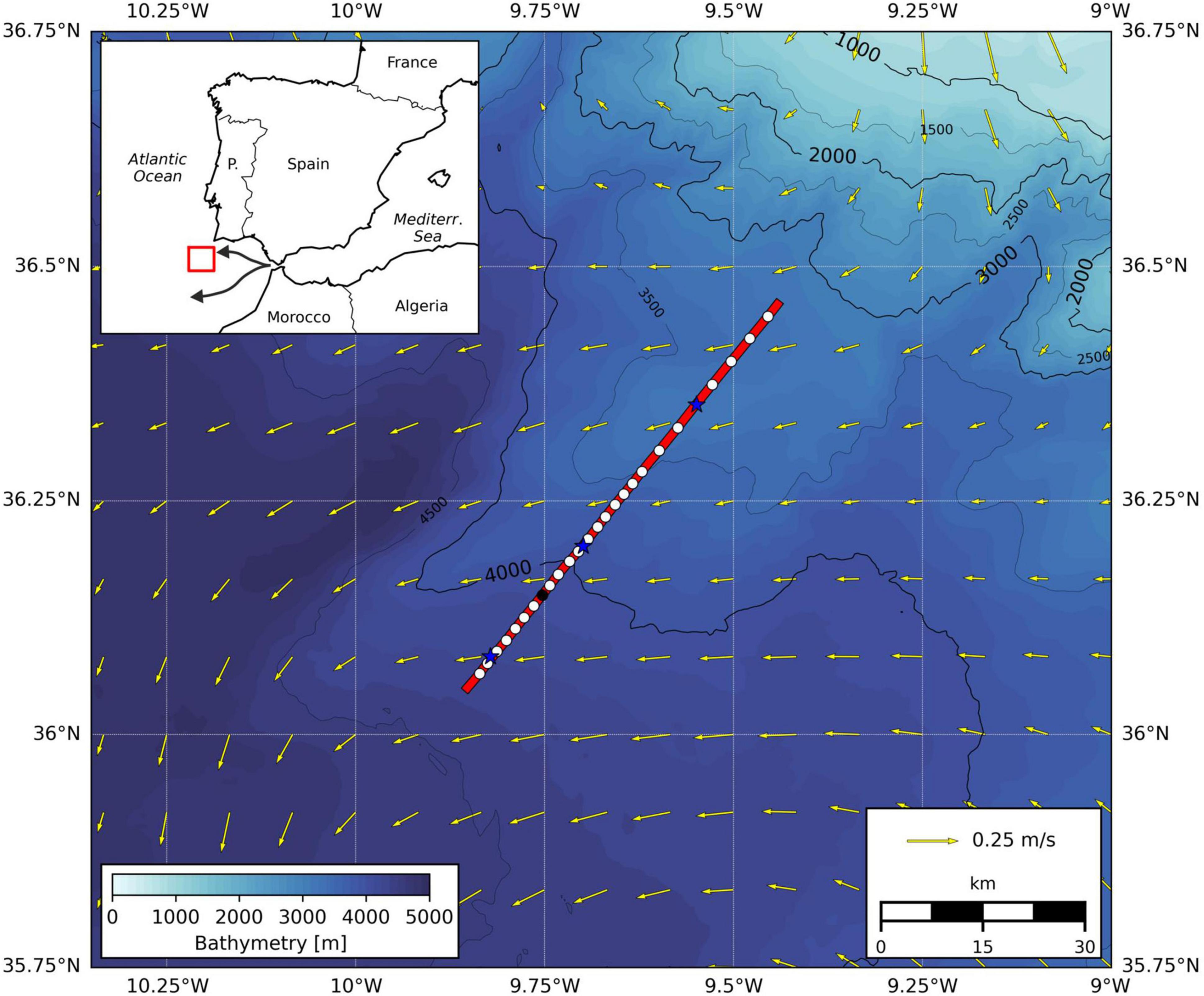
Figure 1. Bathymetry of data collection region. Red line = seismic transect GOLR12; white dots = 24 XBT casts deployed coincident with seismic acquisition; black dot = 1 XCTD cast; blue stars = 3 CTD casts deployed before and after the seismic survey; yellow arrows = surface geostrophic velocity vectors for 7th May 2007. Inset shows location of the research area, and schematic of Mediterranean outflow pathway. Bathymetry was produced from the GEBCO 2020 dataset (GEBCO Bathymetric Compilation Group, 2020). Altimeter products were generated using the Iberia Biscay Ireland Regional Seas Ocean Physics Reanalysis Product with a resolution of 1/12° × 1/12° (https://resources.marine.copernicus.eu/?option=com_csw&view=details&product_id=IBI_MULTIYEAR_PHY_005_002).

FIGURE 2

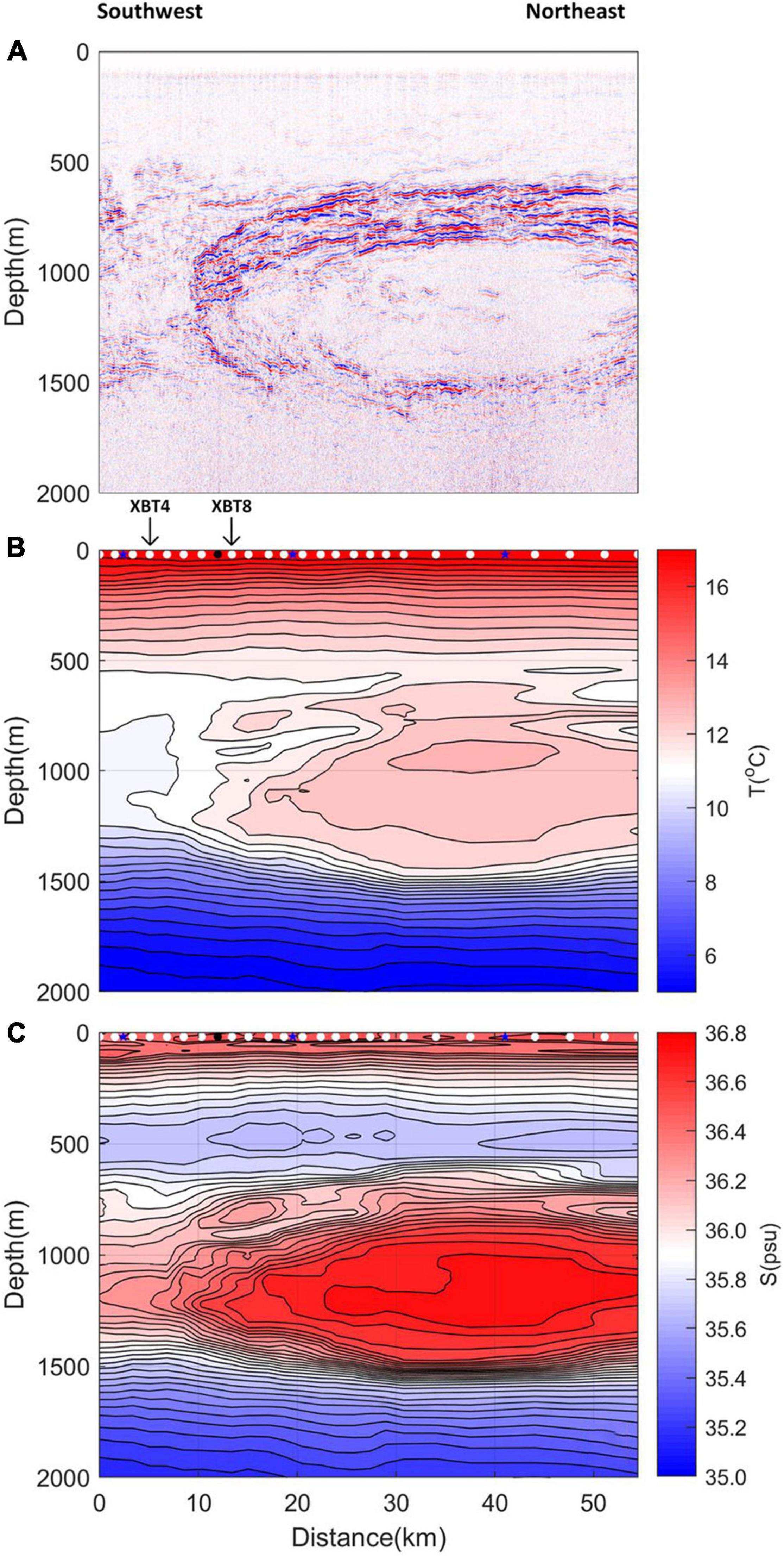
Figure 2. (A) Seismic section of the GOLR12 dataset. Red and blue lines represent reflection horizons caused by temperature and salinity changes in the water column. White (black) dots = 24 XBT (1 XCTD) casts deployed coincident with seismic acquisition; blue stars = 3 CTD casts deployed before and after the seismic survey. (B) Low frequency temperature section built from interpolation of XBT data. A linear interpolation was used with a vertical smoothing (moving average) of 35 m. (C) Low frequency salinity section built from interpolation of salinity estimated from XBT and CTD data following Ballabrera-Poy et al. (2009). Panels (B,C) form the prior model for the MCMC inversion. Note positions of XBT 4 and XBT 8 are indicated on panel (B) (see section “Comparing Inverted Results to Observations”).

Hydrographic data was collected by two ships: the RSS Discovery and the FS Poseidon. In total, twenty-four expendable bathythermographs (XBTs) and one expendable conductivity/temperature profiler (XCTD) were deployed from the RSS Discovery coincident with seismic data acquisition (Figure 1). XBTs were deployed approximately every 2.3 km reaching a depth of 1,830 m. Three CTDs were deployed by the FS Poseidon, along the seismic transect a few hours before or after seismic acquisition. Using the neural network approach of Ballabrera-Poy et al. (2009), the CTD data allowed for the estimation of salinity from XBT data. 70% of the CTD data were used as training data, 15% as validation data and 15% as testing data. Using only CTD data coincident with the seismic line (as opposed to all 43 CTD casts collected on the GO cruise) produced lower errors in the derived salinity values, likely because the local depth-temperature-salinity relationship associated with the meddy was better represented. Low frequency interpolated temperature and salinity sections are shown in Figure 2: these were used to form the prior model for the MCMC inversion.

Markov Chain Monte Carlo Inversion

Following Tang et al. (2016), a Bayesian Markov Chain Monte Carlo (MCMC) approach is used to recover temperature and salinity fields from the seismic data, alongside their probability distributions (i.e., the posterior distribution), at the resolution of the seismic image [i.e., O(10 m)]. In this approach, a probability distribution associated with a prior model is used to iteratively randomly draw N solutions at each inversion point. A likelihood function determines how well each random sample fits the observed data (i.e., seismic reflectivity), and whether to accept or reject the solution. After a sufficient number of iterations (i.e., the “burn-in” period) the posterior distribution converges and fluctuates within a given range. The mean and standard deviation of the posterior distribution, with burn-in-period removed, are used to estimate the final temperature and salinity, and their associated uncertainties (Gamerman and Lopes, 2006). Here, the inversion was conducted on reflectivity values and performed at every seismic reflectivity profile or common midpoint (CMP) and depth coordinate across the seismic section. The Markov chain length, N, was set to 2,000 and the first $\frac{1}{3} N$ iterations discarded as burn-in iterations. The likelihood function of reflectivity, R given the model, m was computed as

L (m | R (C M P, d)) \propto

exp [- \sum \frac{{R_{o b s} (C M P, d) - R_{p r e d} (C M P, d)}^{2}}{2 σ_{e}^{2}}]

where R_obs(CMP,d) and R_pred(CMP,d) represent the measured and predicted reflectivity data at each CMP and depth, and σ_e is the measured data uncertainty. R_obs was computed by summing the high frequency component of the reflectivity, R_{high_freq_seismic}, obtained from the seismic data (band-pass filtered to 10–80 Hz), with the low frequency component (<10 Hz, R_{low_freq_XBT}) deduced using XBT interpolated temperature and salinity fields (Figure 2) following Biescas et al. (2014). As such R_obs = R_{high_freq_seismic} + R_{low_freq_XBT}. R_pred (CMP, d)was computed from the vertical profile of the starting model (R_{low_freq_XBT}), but with the temperature or salinity value at depth, d, sampled from a prior distribution. This prior distribution was obtained using the standard deviation of starting model temperature and salinity values within a vertical 40 m window of d (i.e., the vertical spatial resolution, L₀∼ 40 m, corresponds to a frequency, f_o, of 10 Hz following L_o = c/4f_o, where c = 1,500ms⁻¹is the sound speed (Sheriff and Geldart, 1995). σ_e was estimated as 7.06 × 10^–6, the ambient seismic noise calculated as the standard deviation of seismic reflectivity within an area beneath the meddy where there are no strong seismic reflections. The ambient noise was found to follow a normal distribution. See Tang et al. (2016) for further details of inversion procedures.

Iteratively Improving the Prior Model

As shown later, the success of the MCMC inversion is highly reliant on the accuracy of the low frequency component of the prior model, R_{low_freq_XBT}. A similar conclusion was noted by Tang et al. (2016). To improve the start temperature-salinity model for the inversion, we investigated iteratively updating the prior model at each inverted common mid-point (CMP), using previous inverted results. The seismic survey was broken up into “inversion units,” defined by XBT locations such that each unit was bordered by an XBT profile (XBT_i and XBT_ii) with N_s CMPs, or seismic reflectivity profiles, in between. For each inversion unit, the MCMC inversion process was started at the CMP closest to XBT_i (i.e., CMP 1), with the prior model computed by linearly interpolating data from XBT_i and XBT_ii. Inverted temperatures and salinities at CMP 1 were then combined with XBT_i and XBT_ii, to produce a new prior model. The updated prior model was used for the next CMP inversion, which was conducted at the CMP closest to XBT_ii (i.e., CMP N_s). The process was repeated at CMP 2, CMP N_s -1, CMP 3, CMP N_s-2…, until the whole unit had been inverted: see Figure 3 for a schematic. Inverted results were not incorporated into the prior model if an associated posterior uncertainty anomaly (i.e., compared to a depth moving average of 100 m) was above a chosen threshold of 0.04°C. At each inversion step therefore, the prior model was iteratively updated to incorporate both the hydrographic data and previous inversion results. Recovered temperatures and salinities using the iteratively updated prior model were compared to those using a stationary prior model.

FIGURE 3

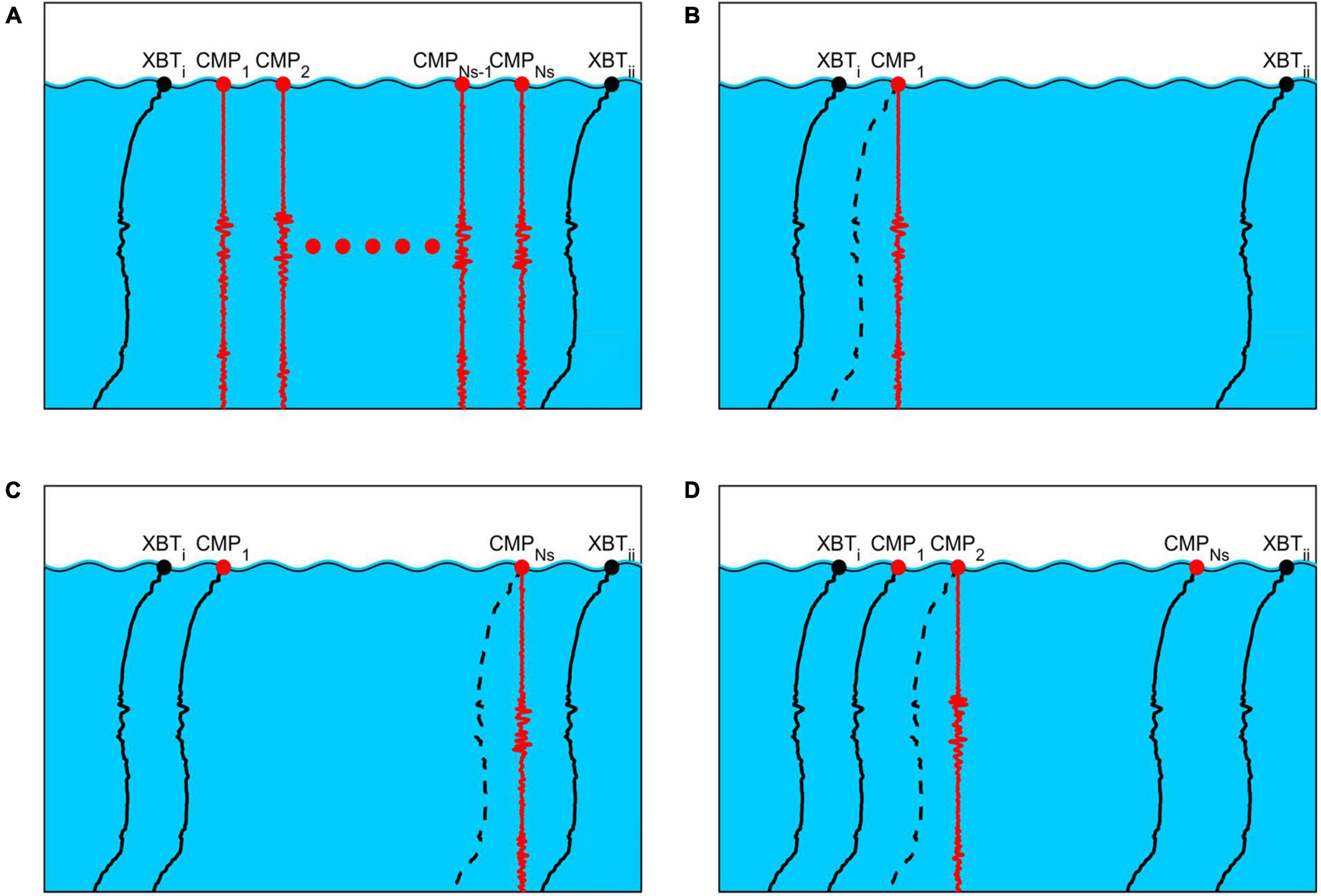
Figure 3. Schematic of inversion unit and iterative MCMC approach. Black dots indicate XBT positions that bound the inversion unit (XBT_i and XBT_ii). Solid black lines represent the prior temperature-depth model as a function of depth. Red dots represent positions of Ns seismic CMPs, and red wiggles show associated seismic reflectivity depth profiles used in inversion. Dashed lines represent newly inverted temperature-depth profiles. (A) Starting data within inversion unit. (B) CMP 1 is inverted using prior model from XBT data. (C) Inverted data from CMP 1 is used to update the prior model. CMP Ns is inverted. (D) Inversion from CMP Ns is used to update prior model, and CMP 2 is inverted. The process is repeated for CMP Ns-2…CMP 3… until the whole inversion section has been processed.

Uncertainty Estimation

Uncertainties introduced to the high-frequency component of the recovered temperature and salinity fields by noise in the seismic data and any mis-alignment of XBT data is accounted for in calculating the standard deviation of the posterior MCMC distribution (Tang et al., 2016). Contamination to the reflectivity field associated with the ringyness of the seismic source and other receiver responses has been minimized by performing a deconvolution on the seismic data using the source wavelet. In this study we also quantify the uncertainty introduced by inaccuracies in the low frequency starting temperature and salinity models. Firstly, the error associated with the estimation of the salinity from XBT temperature data using the non-linear approach of Ballabrera-Poy et al. (2009) was evaluated by applying the technique to CTD-based temperatures. The RMS error between estimated and measured salinities was computed for the 15% of CTD data not used in the model training (with CTD data recorded every 1 m this equates to a total of 6,090 data points, with 914 used for validation). The RMS salinity error was found to obey a normal distribution from which the standard deviation was used to compute the uncertainty. Secondly, errors introduced as a result of the interpolation of XBT data were considered. Starting models were recomputed using 12, 7, 5, and 4 XBTs, corresponding to typical XBT spacings of 4.6 km, 9.1 km, 13.6 km and 18.2 km, respectively. The distribution of RMS errors between the starting model temperature and salinities, and those measured from the removed XBTs were used to estimate the interpolation uncertainty for different XBT spacings (i.e., the standard deviation of the error distribution which was found to follow a normal distribution). For the case of all 24 XBTs (spacing of ∼2.3 km), the error distribution was computed using half the difference of XBT neighboring pairs. We note that the position of reflectors can get distorted and reflection amplitudes weakened by moving water effects (Klaeschen et al., 2009; Vsemirnova et al., 2009; Papenberg et al., 2010). Maximum current velocities in the survey region were ∼0.4 ms^–1 and hence uncertainties associated with moving water to the inverted fields are likely small compared to other uncertainty sources (Papenberg et al., 2010). A summary of the inversion process, along with sources of uncertainties, is shown schematically in Figure 4.

FIGURE 4

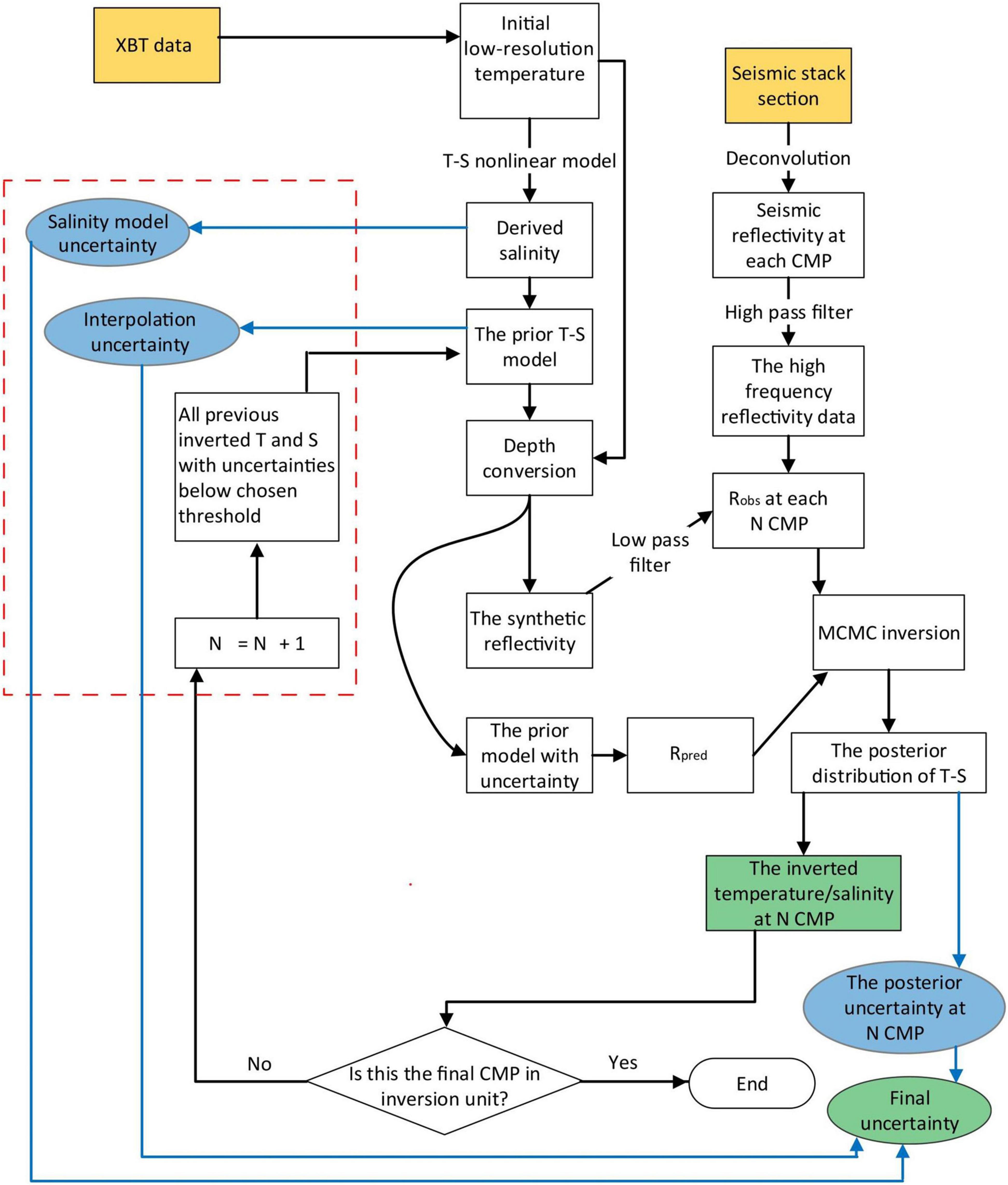
Figure 4. Flow diagram summarizing the iterative MCMC inversion procedure. Rectangular shapes represent processing steps. Yellow rectangles represent the starting points of one inversion loop (input temperature profile and seismic data). Blue circles indicate the uncertainties relating to methods, data or models. Green rectangles represent output of inverted results and their corresponding uncertainties. Stages surrounded by red dashed lines represent updates to Tang et al. (2016). Note that the synthetic reflectivity is calculated from the prior temperature-salinity model following Ruddick et al. (2009).

Results

Markov Chain Monte Carlo Inversion of the Seismic Section

The final recovered temperature and salinity fields, alongside computed potential densities, for the meddy are shown in Figure 5. The meddy shows a distinctive lens-shaped core of warm (∼12.5°C), salty (∼36.7 psu) water between 650 and 1,500 m depth. The meddy core temperature drops smoothly with depth, while salinities appear slightly greater at the core center. Overall the core is stably stratified. Layering filament features with vertical scales of typically 30 m surround the meddy core, where the velocity shear is likely greatest (e.g., Armi et al., 1989). These thermohaline intrusions are more continuous and distinct at the top of the meddy, where they encompass a region of roughly 300 m depth. On the western boundary of the meddy the finescale structures become more disrupted and the erosion of the meddy through mixing with cooler, fresher north Atlantic water is apparent. Fewer filaments are present on the lower surface of the meddy. The dynamics of these imaged thermohaline intrusions and their variability around the meddy core will be investigated in further studies. On the northeast of the section, along the upper edge of the meddy, there is one reflection horizon with anomalously low temperatures, high salinities and unstable density: this region should be interpreted with caution due to the high posterior MCMC inversion uncertainties here (see section “Markov Chain Monte Carlo Inversion Uncertainties”).

FIGURE 5

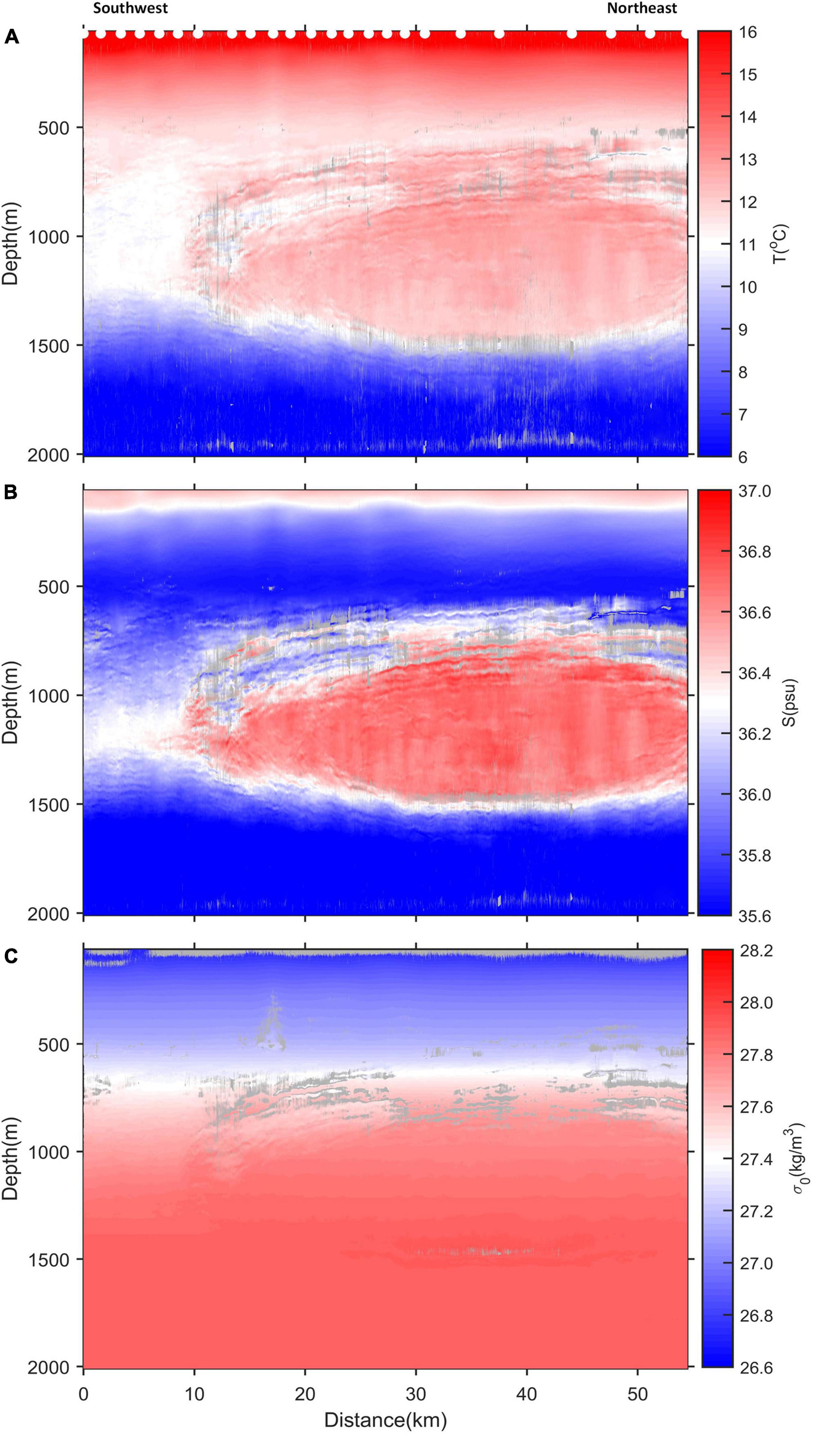
Figure 5. MCMC inversion results of seismic section for (A) temperature, (B) salinity and (C) potential density anomaly. 24 XBTs (white dots) are used to compute the prior model, which is iteratively updated with inversion results. The inversion is performed at every CMP. Seismic data above 60 m depth is discarded due to the contamination from the residual direct wave. No reflectors were present below 2,000 m. Grayed out regions mark areas of high uncertainty (i.e., within the top 5% of uncertainties across the section).

Figure 6 shows an example of the MCMC inversion process at 539 m depth for CMP 2300 (i.e., a transect distance of 8.1 km), located at the midpoint of an inversion unit. The temperature and salinity decrease steadily in the first 300 inversion iterations before stabilizing after about iteration 600 (the “burn-in” period). Comparison of prior and posterior distributions show the reduced uncertainty in inverted compared to initial model temperatures and salinities, with the mean temperature and salinity dropping from 11.6 to 11.4°C and from 35.73 to 35.68 psu after the MCMC inversion.

FIGURE 6

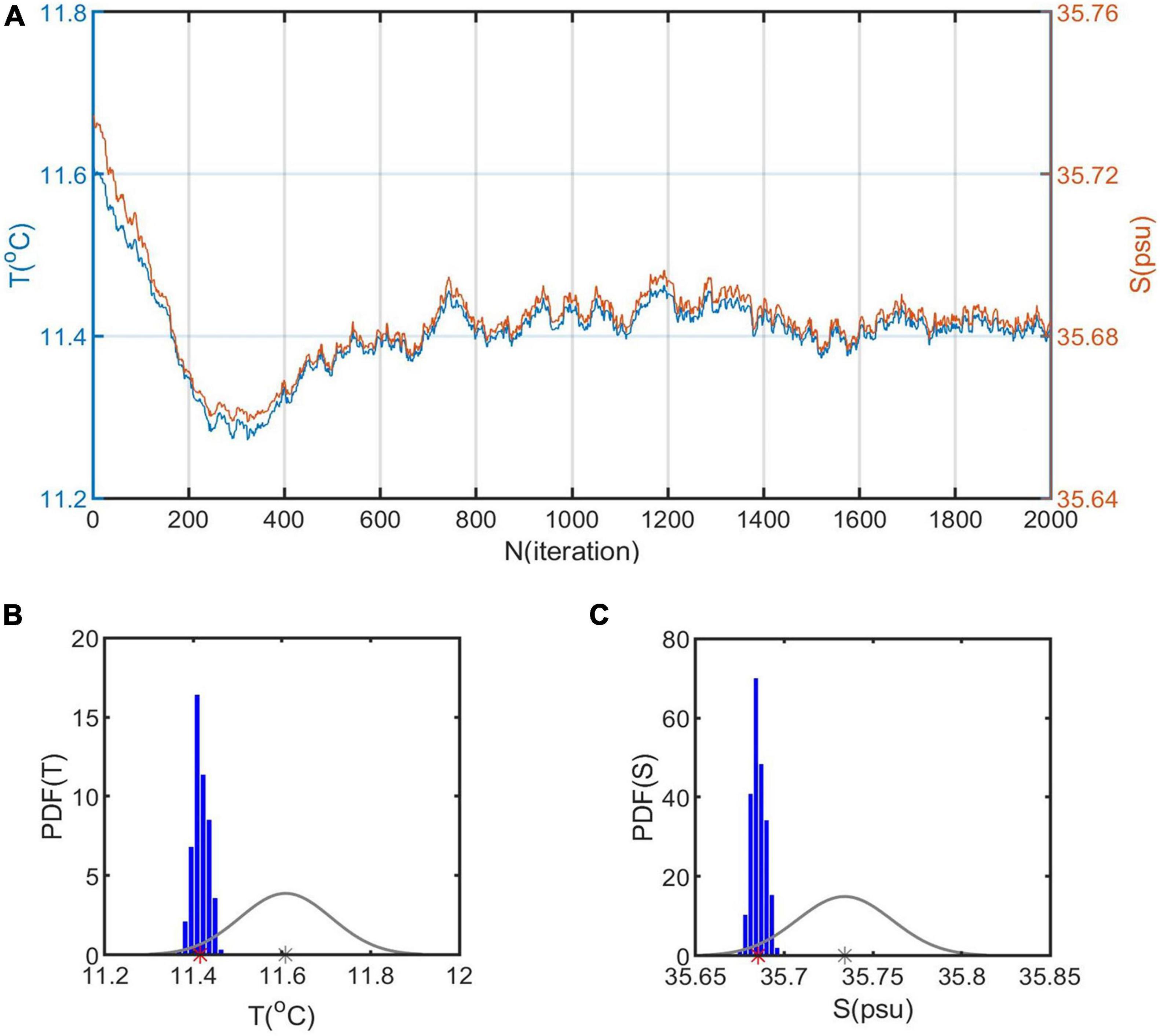
Figure 6. (A) The Markov temperature and salinity chain at depth 539 m, CMP 2300. (B) Associated temperature prior and posterior probability density functions (PDFs). Gray curve = prior distribution of temperature. Gray star = mean of temperature prior distribution. Blue bars = posterior distribution. Red star = the mean temperature of the posterior distribution. (C) As for panel (B) but for salinities.

Markov Chain Monte Carlo Inversion Uncertainties

One of the developments to previous inversions of the GO project meddies [e.g., see Papenberg et al. (2010) and Biescas et al. (2014)] presented here is that the Bayesian framework of the MCMC inversion allows for the posterior uncertainty at each inversion point to be computed and thus the spatial distribution of recovered temperature and salinity uncertainties analyzed. While MCMC posterior distribution uncertainties vary spatially, section averaged uncertainties are used for the uncertainty associated with interpolation of the prior model, and the error associated with estimating salinity from XBT data (see Table 1). The final section uncertainty is shown in Figure 7. Maximum uncertainties of the recovered temperature and salinity are 0.28°C and 0.12 psu, respectively. Regions of higher reflectivity at the meddy boundary tend to correspond to higher uncertainties. Despite the higher signal to noise ratio in these regions, MCMC posterior distribution uncertainties increase due to higher thermohaline variability (Tang et al., 2016). In particular, a short band of high uncertainties most notable in the salinity field is found on the northeastern upper meddy boundary. These high uncertainties are associated with one reflection horizon and indicate the MCMC inversion did not perform as well here, likely due to the high variability in the temperature and salinity at the edge of the meddy and associated disruptions to the reflectivity. Uncertainties in the meddy core are typically 0.15°C and 0.06 psu.

TABLE 1

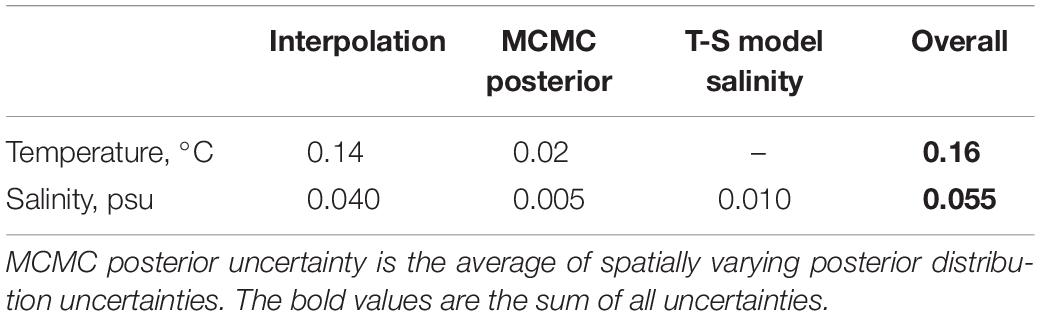
Table 1. Uncertainties across the seismic section for an MCMC inverted temperatures and salinities with all 24 XBTs used to produce the prior model which is iteratively updated with inversion results.

FIGURE 7

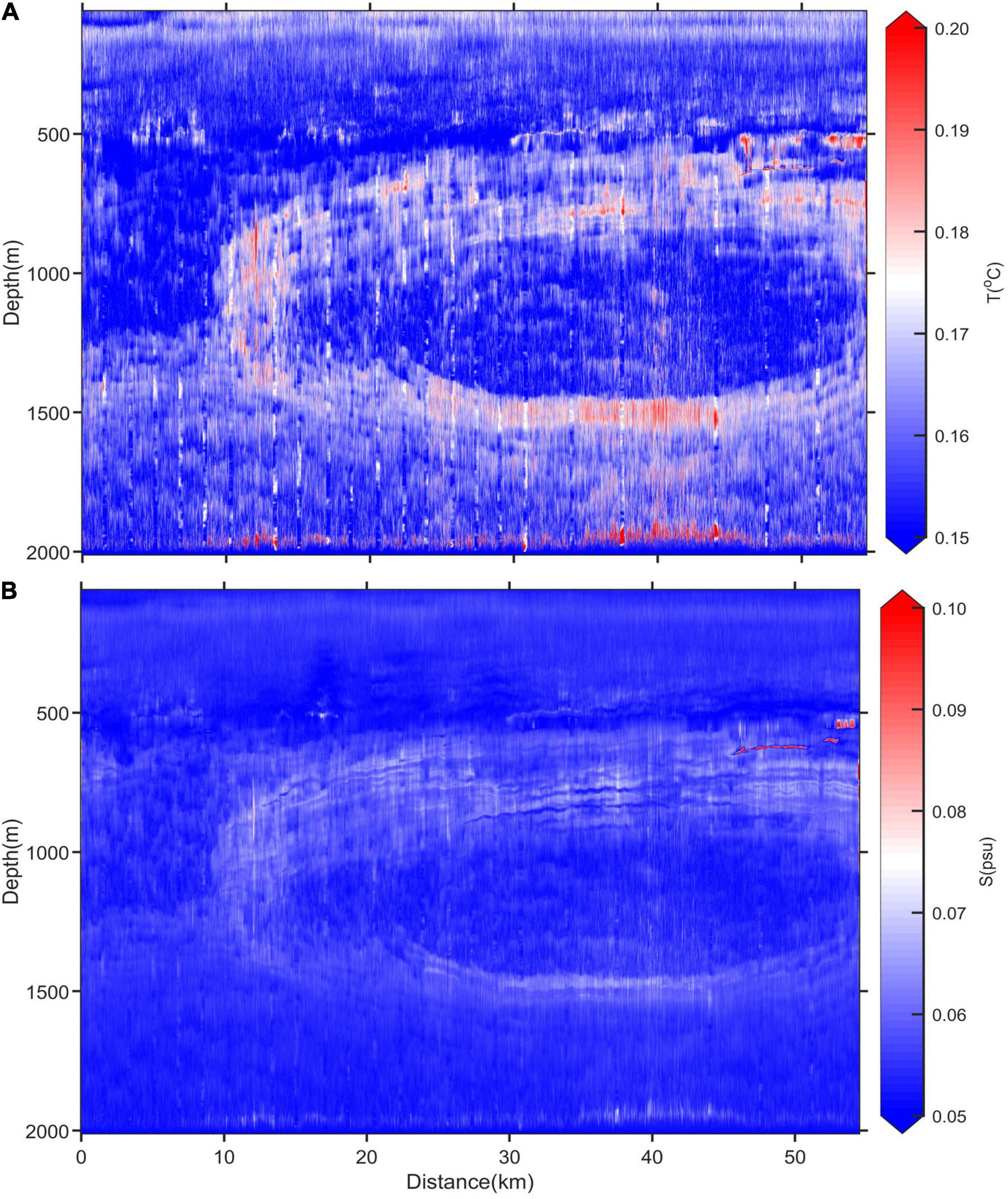
Figure 7. Spatial distribution of final inversion uncertainties for (A) temperature and (B) salinity using all 24 XBTs. Uncertainties include the standard deviation of the posterior MCMC distribution, errors introduced from interpolation of the prior low frequency model, and the uncertainty in estimating salinity from XBT temperature values.

Table 1 summarizes the inversion uncertainties averaged across the seismic section associated with the MCMC posterior distribution, the interpolation used to produce the starting model, and the estimation of salinity from XBT data using the neural network fitting approach. The error associated with the interpolation of the hydrographic data to produce the low frequency prior model dominates the total uncertainty as also found by Biescas et al. (2014). For example, when all 24 XBTs are used to compute the starting model, 88% of the total temperature uncertainty is due to errors associated with the low frequency starting model. The error associated with estimating salinity from XBT data makes up roughly 18% of the total salinity uncertainty. The impact of reduced XBT sampling on recovered temperature and salinity uncertainties is shown in Figure 8.

FIGURE 8

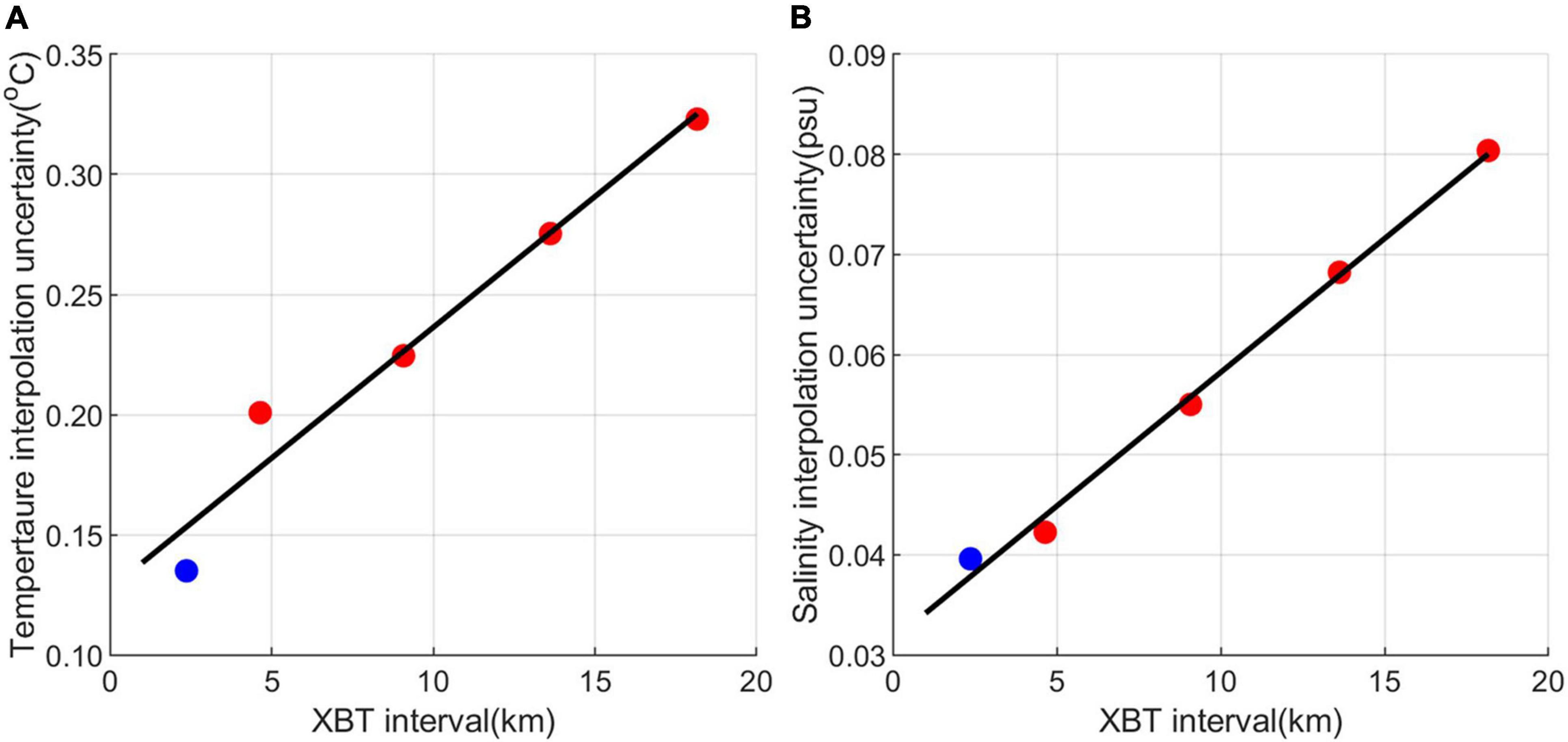
Figure 8. (A) Variation of prior model interpolation temperature uncertainty (for the whole section) with XBT sampling resolution. Blue dot highlights slightly different method used to compute uncertainty when all 24 XBTs are included (see section “Materials and Methods”). (B) As for panel (A) but for salinity uncertainties.

Comparing Inverted Results to Observations

To evaluate results, measured XBT data were compared with inverted values: the inversion was re-run with every other XBT removed, for independent validation of inverted results. Here we show validation examples from two locations on the seismic section: XBT 4, located to the west of the meddy, and XBT 8 which was deployed at the edge of the meddy where horizontally the temperature changes rapidly (see Figure 2 for XBT locations). Results are shown in Figure 9. Outside the meddy (XBT 4) measured and inverted temperatures and salinities are extremely well matched, with RMS error standard deviations for temperature and salinity of 0.14°C and 0.04 psu, respectively. However, the quality of the initial model degrades significantly in regions of rapid temperature or salinity change after removing half of the XBTs. At the meddy edge (XBT 8) inverted temperatures differ from XBT data by more than 1°C at some depths, such as between 1,000 and 1,200 m. The MCMC was found to converge in this region, and the signal-to-noise of the seismic data here is not unusually low. As such it is likely the inaccuracy of the initial model that has resulted in these poor inversion results (Figures 9E–H). Considering the reduced uncertainty associated with increased XBT sampling (Figure 8), inversion results are likely much better at XBT 8 for the case where all 24 XBTs are utilized. An appropriately sampled low frequency prior model is key for accurate inversion results.

FIGURE 9

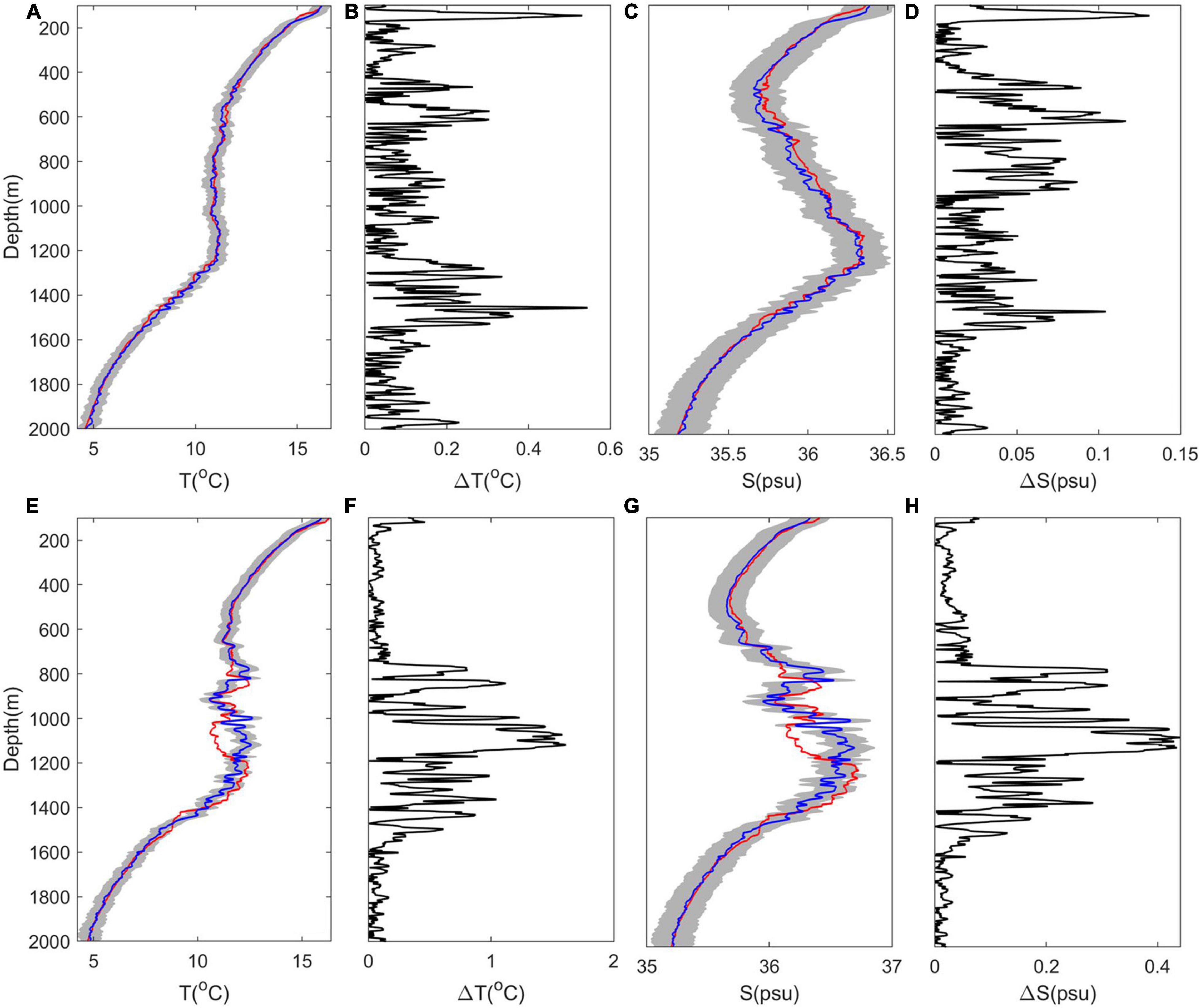
Figure 9. (A) Temperature depth profiles deduced from the MCMC inversion using an iteratively updated prior model computed from half the XBTs (blue) and the observed data computed from the removed XBT 4 (red) to the west of the meddy. Gray shaded regions show 95% uncertainty bands. (B) Differences between inverted and measured XBT temperature at XBT 4. (C,D) As for panels (A,B) but for salinity data. (E–H) as for panels (A–D) but for the XBT 8, located at the edge of the meddy. Note that the edge of the meddy (depths ∼1,100 m), where interpolation errors are particularly high, is one of the regions where the observations do not fall within our 95% uncertainty estimate.

Comparing an Iteratively Updated to a Stationary Prior Model in the Markov Chain Monte Carlo Inversion

Alongside improving the uncertainty estimates of inverted temperature and salinity fields, we have also built on the MCMC inversion methods developed by Tang et al. (2016) by iteratively updating the prior model at each step of the inversion (see section “Materials and Methods”). Comparison of inverted temperature and salinity uncertainties using an iteratively updated prior model to a stationary prior model are shown in Figure 10. Although the prior uncertainties of the two methods are similar, posterior distribution uncertainties (i.e., as computed from the MCMC process) are reduced in the iterative approach. In particular, the more extreme MCMC uncertainties are reduced in the iterative approach as shown by the smaller tails in the uncertainty distributions (Figure 10). The mean posterior temperature and salinity uncertainties using the stationary prior model method are 0.03°C and 0.008 psu compared to 0.02°C and 0.005 psu for the iteratively updated model, implying that inverted results are closer to the field data if an iterative prior model is used. Differences in inverted fields between a stationary and iteratively updated prior model become most apparent when a lower resolution starting model is used with reduced XBTs (as is the case in many seismic oceanographic datasets), as shown in Figure 11. Here MCMC inverted temperatures for a region at the edge of the meddy using a prior model with a reduced XBT spacing of ∼30 km are shown, using both a traditional stationary prior model and an iteratively updated prior model. Note that apart from the uncertainty analysis, the stationary MCMC approach is essentially equivalent to the conventional linearized inversion approach as used by Papenberg et al. (2010) and Biescas et al. (2014). Both inversion approaches are compared to the high-resolution temperature field constructed from all XBTs (i.e., with a spacing of approximately 2 km). The temperature field from the stationary method is found to vary little from the prior model, and displays a far more coherent horizontal structure when compared with both the iterative approach and high-resolution XBT section (for example along the top in the region at depths 600–800 m and transect distance 28–37 km). The stationary prior model inversion thus appears to be highly constrained to the interpolated background starting model. Iteratively updating the prior model with previous inversion results overcomes this constraint, and in many places results in a more representative temperature inversion that reflects the horizontal variability and complexity at the edge of the meddy better. However, we note that there are some regions where the non-stationary approach matches the high-resolution XBT data better, such as just outside the meddy core (e.g., depths 1,200–1,350 m; transect distance 13–20 km) and we find that the mean absolute difference between the inverted results and the high-resolution temperature section for both approaches are comparable. In conclusion, an iterative MCMC approach reduces posterior uncertainties and removes contamination from linear interpolation of the start model, but a high-resolution prior model is still key for reconstructing detailed temperature and salinity fields.

FIGURE 10

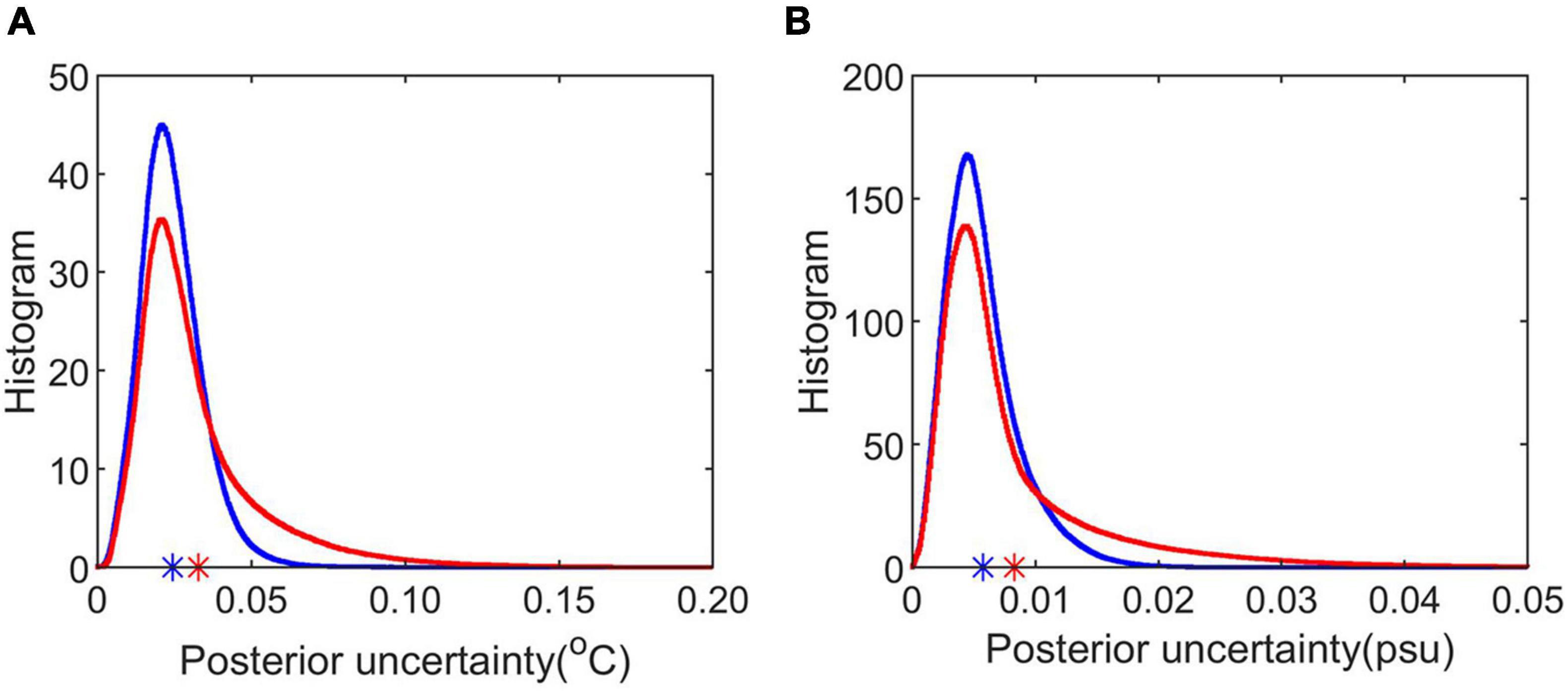
Figure 10. Comparison of stationary and iteratively updated posterior inversion uncertainties. (A) Red (blue) lines show the histogram of posterior temperature uncertainty MCMC distribution for stationary (iterative) prior model. Stars indicate the mean of distribution. (B) As for panel (A) but for salinity uncertainties.

FIGURE 11

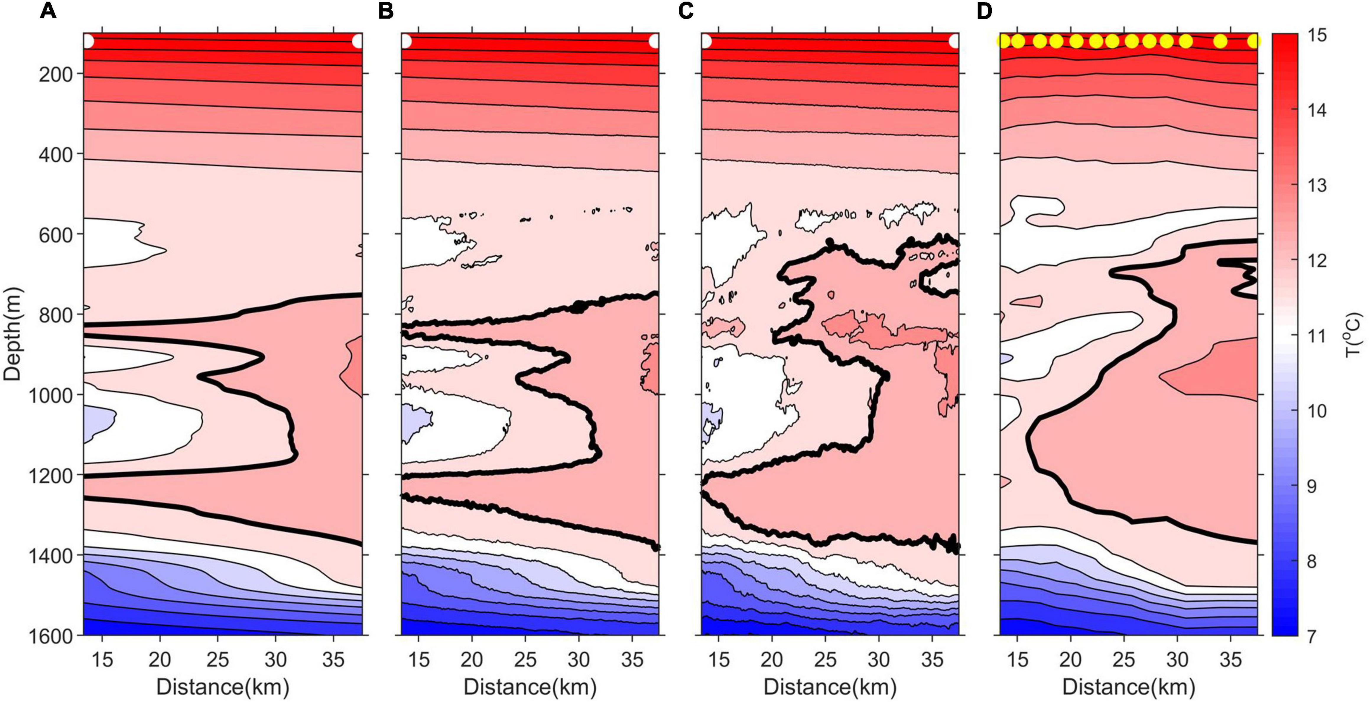
Figure 11. Comparison of MCMC inverted temperature fields using a stationary and iteratively updated starting model. Colored contours show temperature fields, and the thick black line follows the 12.21°C temperature contour, chosen to highlight the meddy structure. (A) Initial reduced XBT-based temperature model used for inversion results shown in panels (B,C) based on interpolation of two XBTs approximately 30 km apart: white dots mark XBT locations. (B) Inverted temperatures using the starting model as shown in panel (A) at each inversion location (i.e., a stationary prior model). (C) Inverted temperature field in which the starting model is iteratively updated at each horizontal position with previous inversion results (see section “Iteratively Improving the Prior Model”). (D) As for panel (A) but the high-resolution temperature field constructing using all available XBT data. Yellow dots mark XBT locations.

Discussion and Conclusion

The Bayesian MCMC approach has been applied to a seismic oceanographic dataset to recover the temperature and salinity of a meddy, with lateral and vertical resolutions of O(10 m). A typical meddy with a stably stratified core of 12.5°C and 36.7 psu, and complex layering and finestructure at the meddy periphery is imaged. Uncertainties in the inverted temperature and salinity results are estimated as 0.16°C and 0.055 psu, respectively. Whilst on face value these uncertainties appear higher than other inversion studies e.g., Papenberg et al. (2010), Biescas et al. (2014) and Tang et al. (2016), here the inclusion of uncertainties associated with both the high frequency and low frequency data components reflect more realistic confidence intervals in recovered temperature and salinity values. Furthermore, the use of the Bayesian MCMC approach has allowed the spatial variability of uncertainties across the meddy to be quantified.

In addition to improved uncertainty analysis, we also investigated the impact of iteratively updating the prior model used in the inversion with previous inverted results, such that MCMC inversion approaches can be used on seismic datasets that may not have coincident high-resolution XBT data [e.g., as in Papenberg et al. (2010) and Biescas et al. (2014)], or continuous reflections as in Tang et al. (2016). The iterative approach is found to both reduce inversion uncertainties and reduce artifacts introduced into the prior model by the interpolation of XBTs. Overall, the iterative MCMC inversion better represents the complex horizontal structure as found around the meddy. However, it should be emphasized that the improvements associated with the iterative approach are secondary to the impact of using a starting model of appropriate resolution: by quantifying and comparing the contribution of uncertainties from different sources we find that the main contributor to the final uncertainty is the low frequency start model as derived from the XBT interpolation. For example, a starting model based on XBT spaced at ∼ 2 km reduces uncertainties in inverted temperature and salinities by 0.16°C and 0.04 psu, respectively, compared to a starting model with XBTs spaced at roughly 18 km. By comparison uncertainties associated with the MCMC inversion of the high-frequency information contained within the seismic data are much smaller, being 0.02°C and 0.005 psu. In conclusion, although the iterative MCMC improves inverted results, an accurate starting model is crucial for reducing the final inversion uncertainty particularly in highly heterogeneous regions such as sub-surface eddies. Other inversion studies also note the necessity of accurate reference models (Biescas et al., 2014; Dagnino et al., 2016; Tang et al., 2016). As such we strongly recommend that high-resolution XBT deployments, ideally deployed every few km, are conducted alongside future seismic studies.

For analysis of legacy data sets lacking coincident, high resolution hydrographic data, or seismic horizons that are not continuous enough to extend prior models as achieved by Tang et al. (2016), other approaches must be adopted to produce spatially improved starting models. One option may be to adopt the method used by Gunn et al. (2018), whereby low resolution temperature fields were extracted from seismic data using the RMS sound velocity picked during velocity analysis of prestack seismic data. This approach could enable the inversion of temperature and salinity fields from seismic data without the need for coincident hydrographic data, useful for analyzing legacy seismic datasets as collected by the hydrocarbon industry. Alternatively, the MCMC inversion approach could be combined with full waveform inversion techniques which despite being computationally expensive are applied directly to pre-stack data, avoiding assumptions associated with seismic stacking techniques and deconvolution (Wood et al., 2008; Dagnino et al., 2016). Furthermore, the combination of MCMC inverted seismic oceanographic field studies, as demonstrated here, with coincident data from underwater autonomous vehicles would provide a complete picture of finescale to mesoscale structures. Seismic experimental set up also impacts the final resolution of inversion results (Hobbs et al., 2009).

This work contributes to the growing approaches to extracting temperature and salinity data from marine seismic surveys, key to understanding finescale and submesoscale oceanic structure and how they relate to larger scale (mesoscale) dynamics. The temperature and salinity fields of the meddy presented here are of high enough resolution and accuracy to be used for further dynamical analysis, such estimating isopycnal displacements and dissipation levels (Sheen et al., 2009; Dickinson et al., 2017) and using spice anomalies to diagnose lateral stirring mechanisms (Klymak et al., 2015). Such data will ultimately improve our understanding of the role that sub-surface eddies play in the distribution of heat, salt, nutrients and other tracers within the ocean.

Data Availability Statement

The raw data supporting the conclusions of this article will be made available by the authors, without undue reservation.

Author Contributions

RH and KLS conceived the idea for the work. WX developed the analysis with guidance from all co-authors. WX conducted the data analysis with some input from QT. WX and KLS wrote the initial draft of the manuscript. RH led the collection of the original in situ dataset. RH, JS, KLS, and QT provided analytical and conceptual advice throughout the project. TE supported data processing and figure production. All authors contributed to the article and approved the submitted version.

Funding

WX was supported by the China Scholarship Council and University of Exeter. This work was supported by the EU project GO (15603) (NEST). QT was supported by the Youth Innovation Promotion Association, CAS (Y202076), and the Rising Star Foundation of the South China Sea Institute of Oceanology (NHXX2019DZ0101).

Conflict of Interest

The authors declare that the research was conducted in the absence of any commercial or financial relationships that could be construed as a potential conflict of interest.

Publisher’s Note

All claims expressed in this article are solely those of the authors and do not necessarily represent those of their affiliated organizations, or those of the publisher, the editors and the reviewers. Any product that may be evaluated in this article, or claim that may be made by its manufacturer, is not guaranteed or endorsed by the publisher.

Acknowledgments

This study has been conducted using E. U. Copernicus Marine Service Information. Seismic sections were produced using OMEGA/Western-Schlumberger, and Seismic Unix software, visualization used MATLAB. Nucleus+ airgun modeling software was provided to Durham University under an academic license by PGS.

References

Armi, L., Hebert, D., Oakey, N., Price, J. F., Richardson, P. L., Rossby, H. T., et al. (1989). Two years in the life of a Mediterranean salt lens. J. Phys. Oceanogr. 19, 354–370. doi: 10.1175/1520-04851989019<0354:TYITLO<2.0.CO;2