 Haibin Song
 Yi Gong
 Shengxiong Yang2,3
- 1State Key Laboratory of Marine Geology, School of Ocean and Earth Science, Tongji University, Shanghai, China
- 2Southern Marine Science and Engineering Guangdong Laboratory, Guangzhou, China
- 3Guangzhou Marine Geological Survey, China Geological Survey, Guangzhou, China
High spatial resolution and deep detection depths of seismic reflection surveying are conducive to studying the fine structure of the internal solitary wave. However, seismic images are instantaneous, which are not conducive to observing kinematic processes of the internal solitary waves. We improved the scheme of seismic data processing and used common-offset gathers to continuously image the same location. In this way, we can observe internal fine structure changes during the movement of the internal solitary waves, especially the part in contact with the seafloor. We observed a first-mode depression internal solitary wave on the continental slope near the Dongsha Atoll of the South China Sea and short-term shoaling processes of the internal solitary wave by using our improved method. We found that the change in shape of waveform varies at different depths. We separately analyzed the evolution of the six waveforms at different depths. The results showed that the waveform in deep water deforms before that in shallow water and the waveform in shallow water deforms to a greater degree. We measured four parameters of the six waveforms during the shoaling including phase velocity, amplitude, wavelength, and slopes of leading and trailing edge. The phase velocity and amplitudes of waveforms in shallow water increase, the wavelengths decrease, and the slopes of trailing edge gradually become larger than that of the leading edge, while the amplitudes of the deep water waveforms do not change significantly and the phase velocities decrease. Our results are consistent with previous studies made by numerical simulations, which suggest the effectiveness of the new processing scheme. This improved scheme cannot only study the internal solitary waves shoaling, but also has great potential in the study of other ocean dynamics.
Introduction
Internal solitary waves are an important oceanographic phenomenon, which affect not only the marine environment, but also affect human activities in the ocean. Internal solitary waves play an important role in energy transfer (Wunsch and Ferrari, 2004) and vertical mixing (Klymak and Moum, 2003; Moum et al., 2003, 2007). Internal solitary waves have proved to be an important mechanism for transport, which often induce sediment resuspension (Bogucki and Redekopp, 1999; Masunaga et al., 2015; Boegman and Stastna, 2019) or change distribution of nutrients and biomass (Haury et al., 1983; Lamb, 1997, 2003; Scotti and Pineda, 2004). In addition, the internal solitary waves can generate strong shear forces, which pose a potential threat to offshore engineering and submarines (Apel et al., 1997; Vlasenko et al., 2000). At present, researchers have made progress in the study of the internal solitary waves both theoretically and observationally, but observations of fine vertical structure and the study of interaction with topography are still insufficient. The South China Sea is a region where the internal solitary waves are well developed (Zhao et al., 2004; Zheng et al., 2007; Cai et al., 2012; Guo and Chen, 2014) and the shoaling internal solitary waves are often observed on the continental shelf-slope. For this reason, the region is an excellent site to study the interaction between the internal solitary waves and submarine topography. Therefore, we decided to use this region to develop a seismic data processing scheme that can study the evolution of the internal solitary waves.
Propagation of the internal solitary waves onto the continental slope is a complex dynamic process. When the internal solitary waves propagate into shallow water, the waveform will deform due to the imbalances between non-linear and dispersion effects. During the shoaling process, the internal solitary waves possibly transform from a depression wave to an elevation wave (Liu et al., 1998) and may be breaking due to mixing (Aghsaee et al., 2010) or form vortices in the core (Lamb, 2002). These processes have been verified in numerical (Holloway et al., 1997; Liu et al., 1998; Zhao et al., 2003; Grimshaw et al., 2010) and physical laboratory simulations (Boegman et al., 2005; Cheng and Hsu, 2010) and observed by means of mooring, high-frequency acoustics, and remote sensing (Orr and Mignerey, 2003; Zhao et al., 2003; Lynch et al., 2004; Bourgault et al., 2007; Shroyer et al., 2008; Fu et al., 2012). However, these observations of the shoaling processes are inadequate, since the observational techniques are unable to visualize the evolution and internal fine structure of the internal solitary waves. High-frequency acoustics can only observe a few scattering interfaces. More importantly, these methods cannot be used to observe the interactions between the topography and internal solitary waves. These observational constraints have limited our understanding of shoaling process of the internal solitary waves.
With the development of seismic oceanography (Holbrook et al., 2003), seismic reflection surveying has been applied to study various oceanographic phenomena including fronts (Holbrook et al., 2003; Tsuji et al., 2005), water mass boundaries (Nandi et al., 2004), mesoscale eddies (Pinheiro et al., 2010), internal waves (Holbrook and Fer, 2005; Bai et al., 2017), the Mediterranean undercurrent (Buffett et al., 2009; Biescas et al., 2010), and submesoscale processes (Sallarès et al., 2016; Tang et al., 2020). More recently, seismic reflection studies have now been used to look at the evolution of oceanic processes over time (Dickinson et al., 2020; Gunn et al., 2020; Zou et al., 2021). This method has high spatial resolution. The vertical resolution can be less than 10 m and the lateral resolution is approximately 6.25 or 12.5 m. Such vertical resolution is close to the scale of the “step-like” vertical profile of temperature and salinity induced by double diffusion in some areas (Magnell, 1976), so seismic oceanography can observe the internal fine structure of water column (Geli et al., 2009). This high resolution ensures that fine structure of the shoaling internal solitary waves is observable by using the seismic reflection method. However, conventional processing schemes of seismic data are not conducive to imaging the motion and evolution of the internal solitary waves, since they yield a single, static image of the water column.
In this observational contribution, we use an adapted acoustic method to report the parameters of the internal solitary waves at different stages of their shoaling. This methodology provides dynamic and high-resolution observations of internal solitary waves (ISWs) that are difficult to otherwise obtain. We hope that such observations can be used to improve theoretical understanding of these phenomena in the future. We improve the processing scheme of seismic data and obtain a series of images (i.e., a time-lapse) of the shoaling internal solitary wave in the northern South China Sea. These images clearly record the evolution of internal structure, according to which we analyze the process of waveform deformation and the influence of topography on the internal solitary wave. In section “Data and Methods,” we introduce the seismic data used in this study and the improved processing scheme. The description of wave properties is given in section “Results.” The shoaling process is analyzed in detail in section “Discussion.” Finally, the concluding remarks are presented in section “Conclusion.”
Data and Methods
Seismic Data Acquisition and Buoyancy Frequency
The Guangzhou Marine Geological Survey acquired a set of two-dimensional (2D) multi-channel reflection seismic data in the South China Sea near the Dongsha Atoll in the summer of 2009. The streamer has a total length of 6 km and contains 480 channels. The trace interval is 12.5 m and the sampling interval is 2 ms. The energy generated by airgun sources has a total volume of 5,080 in3 (1 in = 2.54 cm) and the dominant frequency of the wavelet is 35 Hz. The shot interval is 25 m and the shot time interval is about 10 s. The minimum offset is 250 m. We found the shoaling internal solitary wave on the seismic line Ls, whose location is shown by the red line in Figure 1. The seismic line is located on the continental slope and the slope of the topography is gentle. The observation direction is from southeast to northwest, which is almost the same as the propagation direction of most internal solitary waves near the Dongsha Atoll (Alford et al., 2015). Temperature and salinity measurements from reanalysis data are used to calculate a local buoyancy frequency profile (Figure 1B). The reanalysis data are provided by the Copernicus Marine Environment Monitoring Service (CMEMS) in daily averages. We extract data from the summer of 2009 that are close to the location of the internal solitary wave.
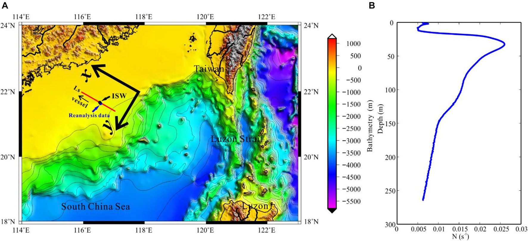
Figure 1. (A) The observation location and bathymetry. The red line is location of seismic section (Ls). The black dot is the location of the internal solitary wave in seismic section. The blue dot is the location of reanalysis data. The arrow indicates the direction of vessel. (B) The buoyancy frequency estimated from reanalysis data.
Typical Seismic Section Processing
The processing scheme of stacked seismic section includes the definition of geometry, direct wave attenuation and noise removal, common midpoint (CMP) gathers sorting, velocity analysis, stacking, and migration (Ruddick et al., 2009). Firstly, we define the survey geometry to create a coordinate system for seismic data. Secondly, we apply a high-pass filter to remove low-frequency background noise and attenuate the direct waves by using a median filter. Thirdly, we sort the shot gathers into CMPs and perform a velocity analysis. We use the results of the velocity analysis to apply a normal moveout (NMO) correction to the CMP gathers, so that the reflection events become flat and can be stacked. Stacking means that adding all the tracks in each CMP gather to form one trace. Finally, we implement poststack migration to improve the imaging accuracy of the stacked seismic section. Yilmaz (2001) describes a more detailed description of seismic reflection processing.
Improved Seismic Section Processing
Multi-channel reflection seismic data will cover a section multiple times during the acquisition, so that we can image the water column multiple times to study the motion of it (Sheen et al., 2012). However, poststack sections generated by the traditional processing schemes require multiple receiver channels to be stacked in order to improve signal-to-noise ratio (SNR). This operation can neither visualize the motion of water column nor fine structure changes during the motion. In order to utilize the multiple coverage information in the seismic data, we resort the CMPs into a number of common offset gathers (COGs), where the offset is the distance between source and receiver. Each COG can be considered as a snapshot of water column. In this way, the motion of water column can be visualized as an animation.
Processing schemes for COG migrated sections are the same as those for conventional stacked seismic section, except that the NMO correction is not applied and CMPs are not stacked. After the third step in section “Typical Seismic Section Processing,” the COGs are resorted from the CMPs according to the offset and a prestack time migration is applied to the COGs. After completing the above steps, a series of COG migrated sections can be obtained.
Two key points are worth noting here. Firstly, as offset increases, the high frequency components in the seismic data will attenuate, which affect imaging quality. To reduce this attenuation, we use a low-pass filter to limit the frequency of all the COGs to less than 80 Hz, so that seismic data of all the COGs are normalized to the same frequency band. Secondly, the imaging range of each COG migrated section is not always the same. Thus, it is necessary to select COG migrated sections with the same CMP range. To ensure these conditions are met, we selected COGs every four channels from the 3rd to the 95th channel and obtain a total of 23 groups of COG migrated sections. Then, by arranging these COG migrated sections according to offset, a series of images, which map the motion of water column over time, can be obtained.
Waveform Characteristics Estimate From Seismic Section
Some waveform characteristics can be directly obtained from the seismic section such as amplitude, wavelength, and the slopes of the front and rear edges of the internal solitary wave. Seismic sections reflect the vertical gradient structure of temperature and salinity (Ruddick et al., 2009) and we refer to this structure as reflective interfaces. Usually, reflective interfaces are parallel to isopycnal surfaces (Holbrook et al., 2003; Sallarès et al., 2009); therefore, they can be traced to extract information about the internal solitary waves. In Figure 2, the black and white stripes indicate the position of an example of reflective interface at a depth of 130 m. The adjacent black and white stripes are caused by the signature of the source rather than changes in ocean properties and we call them seismic events. So, to track the seismic events, we only trace one color stripe. Now, with the isopycnal surface of the internal solitary wave, we can estimate its amplitude, wavelength, and the slope of its leading and trailing edges. Note how these parameters change with depth. In this way, we can use seismic data to study the vertical structure of the internal solitary waves (Gong et al., 2021).
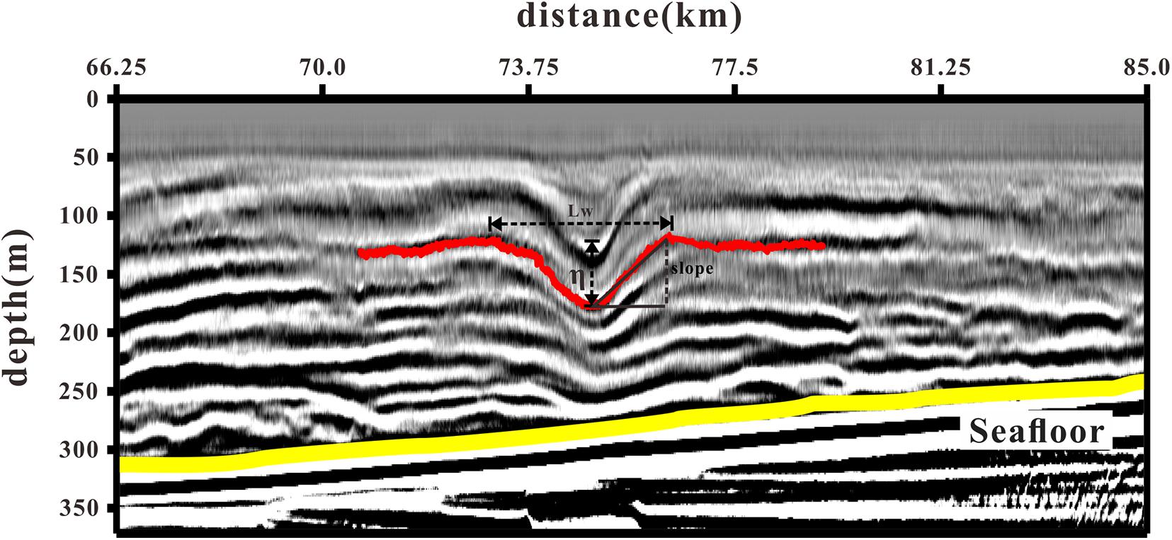
Figure 2. Schematic diagram of amplitude (η), wavelength (Lw), and the slope of the leading and trailing edges (slope) calculation. The red line is one of the seismic events. The yellow line indicates the seafloor.
Wave Phase Velocity Estimate From Prestack Seismic Data
The method to estimate the section velocity of the reflection events is based on prestack seismic data and has been successfully applied to the phase velocity estimation of first mode and the second mode internal solitary waves (Tang et al., 2015; Fan et al., 2021). We first trace the same reflection event of an internal solitary wave from a series of COG sections (the black line in Figure 3). Then, we record the shot number and CMP number of a fixed reflection point on these events, which can be easily read from prestack seismic data. It should be noted that the selected reflection point must be a feature that is not affected by seismic imaging such as the trough or crest of the internal solitary wave (the black dot in Figure 3). The change in the shot number of the reflection point represents the change in time and the change in the CMP number represents the change in distance. Then, the phase velocity of the internal solitary wave can be expressed as:
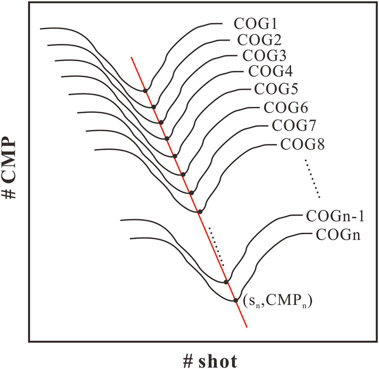
Figure 3. Schematic diagram of calculating the internal solitary wave phase velocity by using pre-stack seismic data.
where, the dCMP is the change in CMP number, ds represents the change in shot number, and dt is the shot time interval.
Results
Internal Solitary Wave in the Stacked Seismic Section
We found a first-mode depression internal solitary wave in seismic line Ls. As shown in Figure 4, the internal solitary wave only has one concave downward waveform. The observation direction is from southeast to northwest, which is consistent with the movement direction of the internal solitary wave. The stacked section is plotted as if the internal solitary wave was propagating from left to right. In Figure 4, the internal solitary wave was shoaling onto the continental slope.
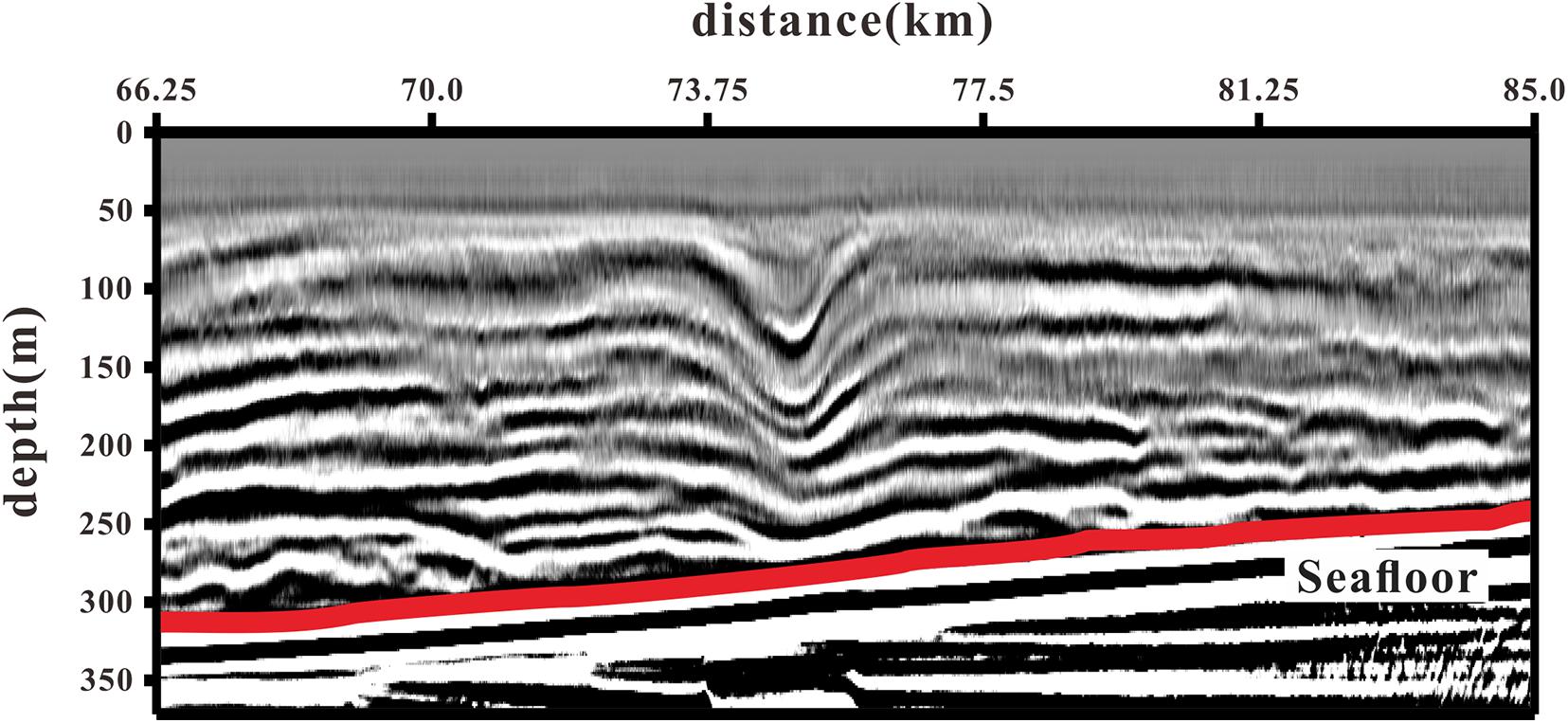
Figure 4. Stacked section of the internal solitary wave. The red line represents seafloor.
A demarcation of the shoaling process is the “transition point.” Before the transition point, the structure of the internal solitary wave will not change much, while after the transition point, the internal solitary wave reverse polarity or break due to mixing. In the two-layer ocean model, the transition point is defined as the position where the pycnocline is close to the mid-depth of water (Grimshaw et al., 2010). The pycnocline depth can be determined by the depth of the extrema of the buoyancy frequency (Liao et al., 2014). According to Figure 1B, the maximum buoyancy frequency is about 37 m deep, which is not within the observation range of the seismic section. According to the two-layer model theory, the depth of the “transition point” should be 74 m, so that the internal solitary wave observed has not yet reached the “transition point.”
The seismic events show continuity over 20 km, which indicate that the stratification is stable. However, the seismic events near the seafloor have bifurcated and broken due to the interaction between the internal solitary wave and topography. According to the study of the vertical structure of the internal solitary wave (Geng et al., 2019), the maximum amplitude of the internal solitary wave is 70 m, which is located at a water depth of 100 m. As the water depth increases, the amplitude gradually decreases. According to Chen et al. (2019), the maximum amplitude of the mode-one internal solitary wave found near the Dongsha Atoll is 87 m, which is similar to the amplitude of the internal solitary wave. In addition, Ramp et al. (2004) observed many internal solitary waves in the east of Dongsha islands and they showed that the amplitude of the internal solitary waves ranged from 29 to 140 m. We conclude that seismic reflection data are a useful and accurate tool to observe the internal solitary wave amplitudes.
Waveform Evolution of the Internal Solitary Wave
Eight time-lapse images of the internal solitary wave are shown in Figure 5. Each image is of the same location, but separated by about 47 s (total observing time of 23 COGs is 18 min). It can be seen from the figure that the shape of waveform in shallow water changed more dramatically than that in deep water. As the offset increases, the reflections in shallow water gradually weaken at the leading edge. In the large offset COG migrated section, the shallow parts of reflection were cutoff due to the large stretching effect of NMO at these offsets, so that the events gradually became indistinct. Due to the fact that the increasing offset resulted in increasing frequency attenuation of seismic data (the raypath increasing), the events in the large offset COG migrated sections had become thicker.
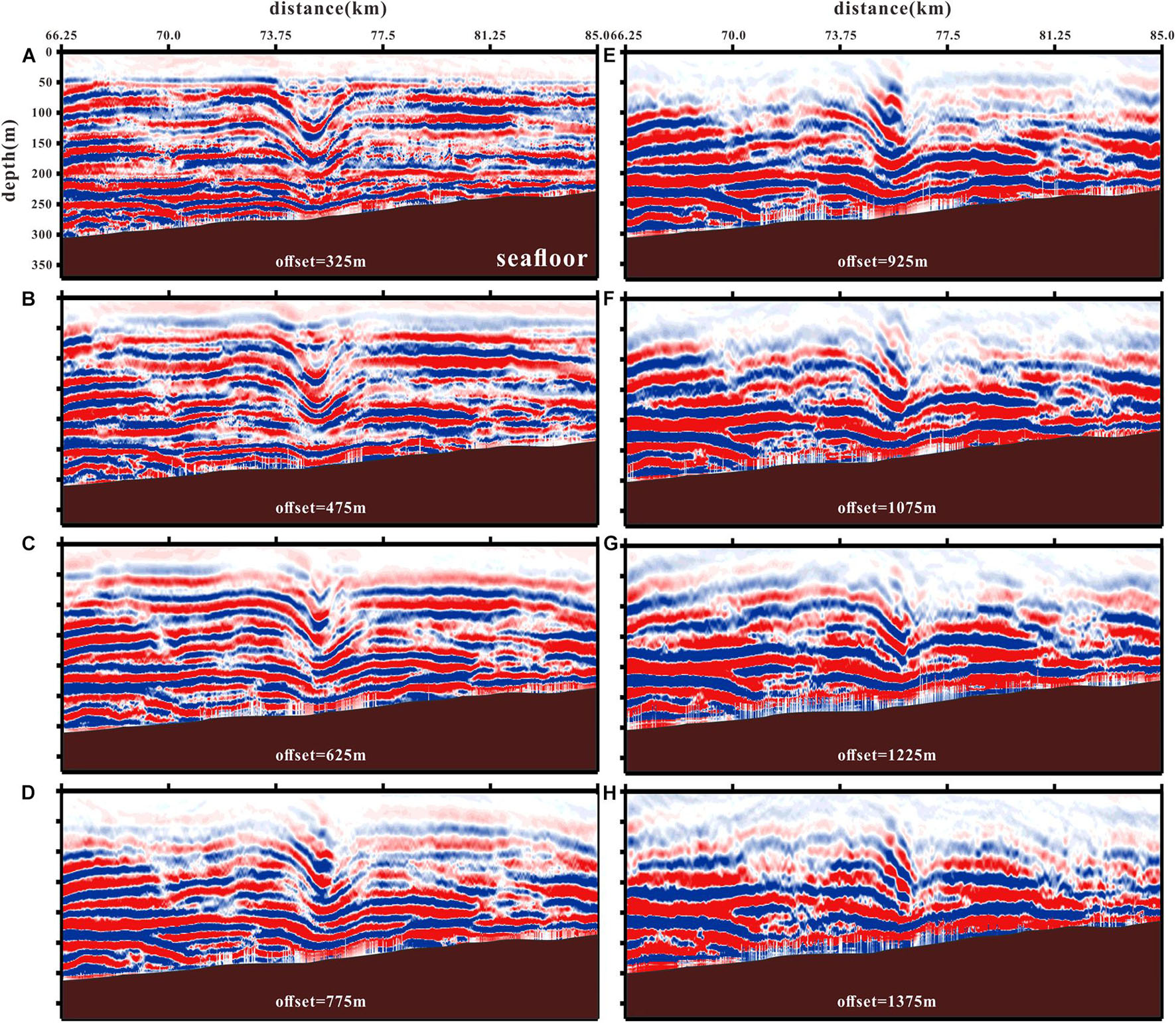
Figure 5. (A–H) Common offset gather (COG) migrated sections with different offsets. For conciseness, only eight sections are shown out of 23 collected. The brown areas represent topography. Seismic section displayed in color and red events are traced to study the internal solitary wave waveforms.
To investigate the waveform evolution in more detail, we pick six seismic events from the eight COG migrated sections (Figure 5), which are shown in Figure 6. Those seismic events represent the waveforms at six different depths. As shown in Figure 6A, as the internal solitary wave moved rightward on the slope, its rear edge shallowed and its slope increased, while the leading edge gradually became flat and the slope decreased. The shape change of waveforms at the different depths is clearly different. In Figures 6B–G, the shape change of each waveform can be viewed, respectively. The first waveform (Figure 6B) was somewhat symmetrical in the first four frames of the image and changed significantly from the fifth frame. In frame 5, the depth of leading edge increased and the shape became flat. An abnormal reflection like “knotting” appeared in the trough. The trailing edge became shallower and the slope increased. Subsequently, in frame 6, the trailing edge continued to become shallower and there was a break in the trough, which resulted in leading edge reflection missing. The broken waveform in frame 7 was connected to the leading edge of the third waveform below and formed a complete new waveform again. There is no first waveform in the frame 8 image because it cannot be accurately identified in the corresponding COG migrated section. The second waveform (Figure 6C) is similar to the first one. The shape of waveform changed from a somewhat symmetrical shape to one with increasing trailing edge slope and decreasing leading edge slope. Eventually, the leading edge broke and the trailing edge connected to the third waveform. The third waveform (Figure 6D) maintained a good symmetry in frame 1 to frame 6 and the change started in frame 7. In frame 7, the waveform was broken and connected to the fourth waveform in frame 8. Except for breaking in frame 8, the fourth waveform (Figure 6E) remained intact in the rest of frames. This waveform is close to the seafloor and the phenomenon that trailing edge slope is larger than leading edge slope already appeared in the first frame. The fifth waveform (Figure 6F) and the sixth waveform (Figure 6G) did not change significantly and there was almost no change in the shape, except for the wave moving up-slope in all the eight frames.
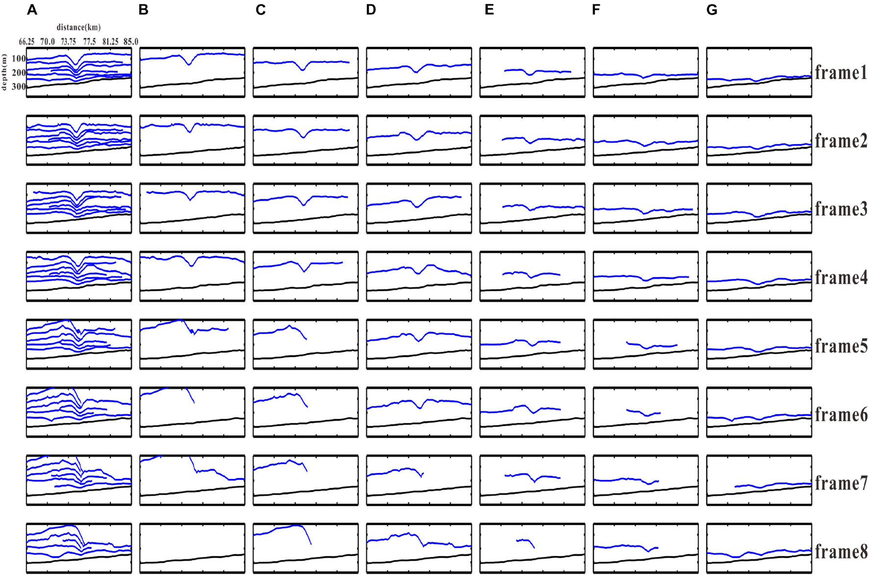
Figure 6. Events (blue lines) picked from COG migrated sections showing the shape change of waveform. (A) Full six waveforms at different depths. (B–G) Separate display of the first to sixth waveform.
Phase Velocities of Waveforms
We measured four parameters of the picked six waveforms in 23 COG migrated sections, which are phase velocity, amplitude, wavelength, and slopes of the leading and trailing edge. The data of the four parameters are shown in Table 1. The phase velocity is calculated by tracing the trough of seismic events in CMP-shot coordinates, which have been converted into distance-time coordinates (Figure 7). In this study, we traced the trough to calculate the phase velocities of the six waveforms. It can be seen from the figure that the phase velocities of the six waveforms are different. The first waveform (Figure 7A) had two different motion regimes, i.e., there was an obvious acceleration in the range of 9–10 km and the phase velocity accelerated from 1.23 (± 0.05) to 2.38 m/s (± 0.55). This acceleration was caused by a large deformation after the waveform was broken. The second (Figure 7B) and the third waveform (Figure 7C) had the same situation, but their phase velocities were different. The phase velocity of the second waveform changed from 1.13 (± 0.05) to 2.44 m/s (± 0.57), while the phase velocity of the third waveform changed from 1.39 (± 0.06) to 2.07 m/s (± 0.55). The fourth (Figure 7D) and the fifth waveform (Figure 7E) did not show any obvious acceleration and their phase velocities were 1.66 m/s (±0.24) and 1.46 m/s (±0.13), respectively. The sixth waveform (Figure 7F) is unique and its phase velocity was reduced from 1.23 (±0.08) to 0.89 m/s (±0.03). Since the sixth waveform was closest to the seafloor, this deceleration might be caused by the friction between the seafloor and internal solitary wave. Comparing the phase velocities of each waveform, we show that the shallower the waveform depth, the more the phase velocity increases. The increase in phase velocity is related to the enhancement of non-linearity, so that the shallow waveform is more susceptible to non-linear effects. The phase velocity of the waveform near the seafloor decreases due to the interaction between the internal solitary waves and seafloor.
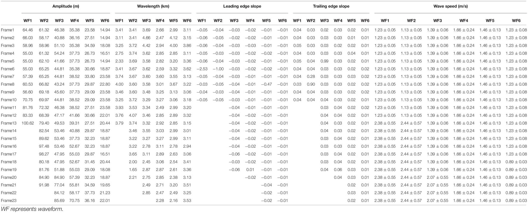
Table 1. The four parameters of the internal solitary wave calculated from seismic data.
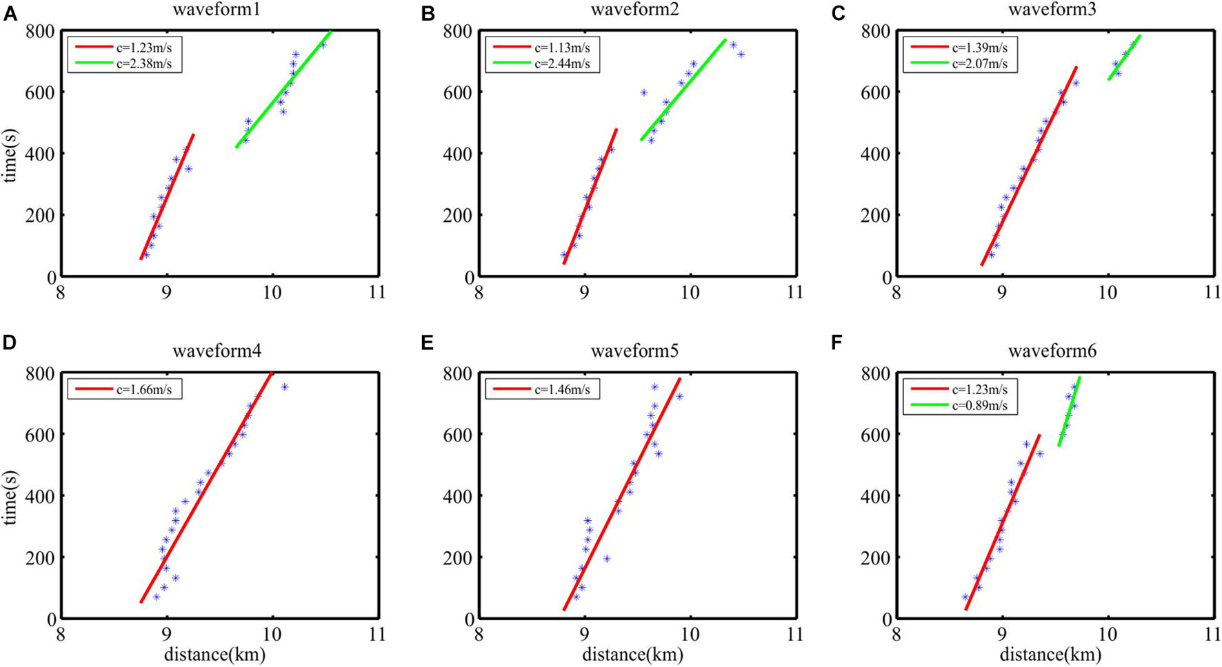
Figure 7. Linear fitting in phase velocity calculation process of the six waveforms. (A–F) The blue asterisks indicate the trough of waveform. The red and green lines are fitting lines of blue asterisks. The common midpoint (CMP)-shot coordinates have been converted into the distance-time coordinates, so that the slope of fitting line is the phase velocity. The red and green lines are different fitting of asterisks, which indicate that the internal solitary waves travel in different phase velocity.
Amplitudes and Wavelength of Waveforms
Figure 8 shows a distribution diagram of amplitudes of the six waveforms. Since the leading edge gradually flattened when the internal solitary wave was shoaling, we defined the vertical distance between the trough and trailing edge as amplitude. It can be seen from the figure that the amplitudes decreased with the water depth increasing and this rule had been maintained during shoaling process of the internal solitary wave. As it is shown by the fitted straight line of amplitudes in Figure 8, the amplitude of each waveform gradually increased when the soliton was shoaling. Numerical simulation results show that the shoaling effect will cause the amplitude of the internal solitary waves to increase in the uphill topography (Cai et al., 2002; Cai and Xie, 2010), which is consistent with our observations. However, the growth rates of the six waveforms were different. As the water depth increased, the growth rate of amplitude gradually decreased.
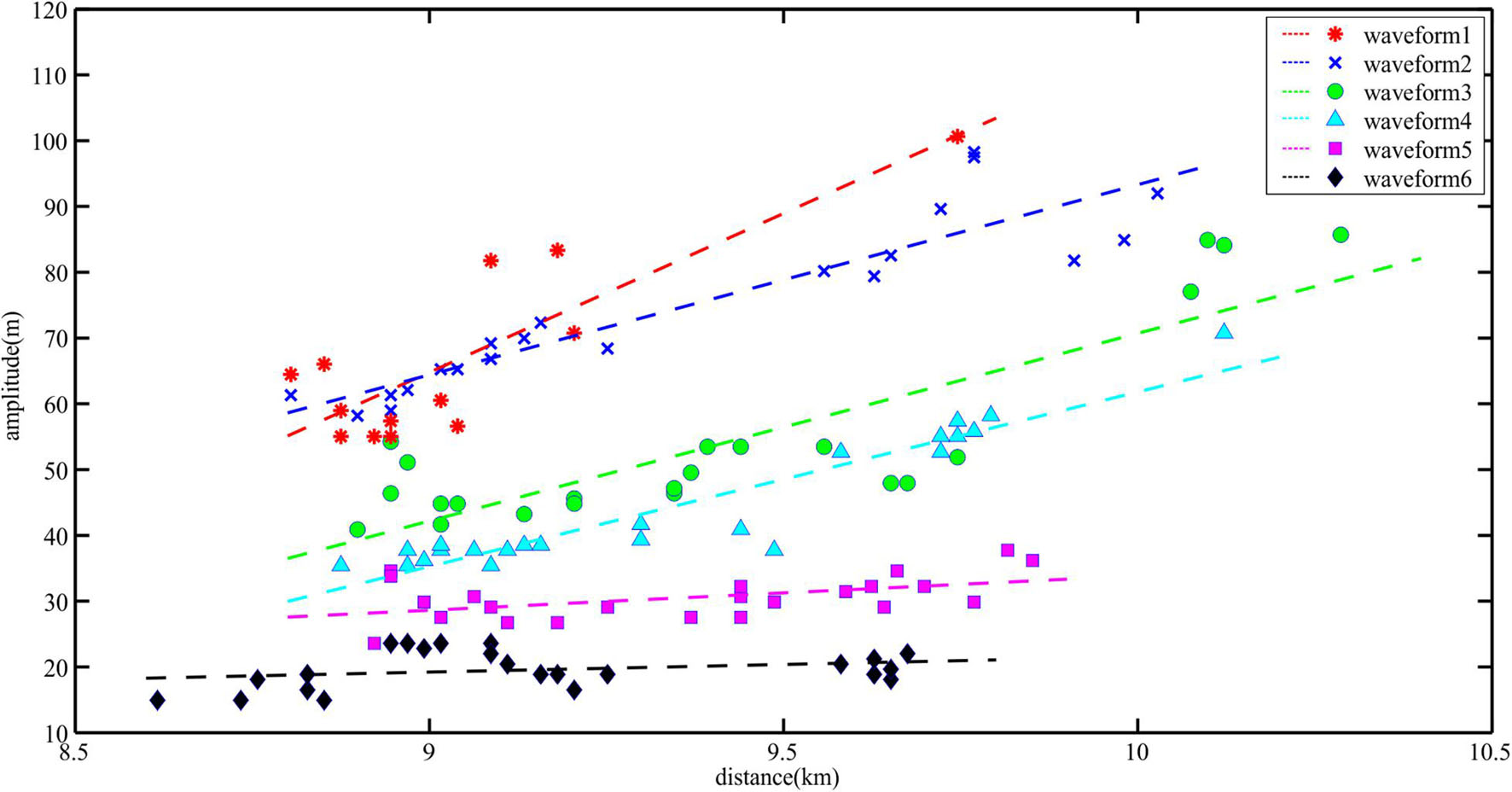
Figure 8. The change in amplitudes of the six waveforms. The amplitudes picked from different waveform are shown by colored scatters. The lines are linear fitting of the marks with same color. The meaning of each colored mark is shown in the upper right legend. The internal solitary wave is moving forward along the X coordinate.
We counted the wavelengths (apparent wavelengths) of the six waveforms, which are shown in Figure 9. It should be noted that the seismic data will be affected by the Doppler-like effect (Bai et al., 2017), so that there is an error between the wavelength picked from seismic section and the true wavelength. In this study, we only discuss the change of wavelength. Since the leading edge of the first and second waveforms in part of COG migrated sections are so flat that we cannot accurately calculate the wavelength, the sample points of the first and second waveforms are less than 23. In Figure 9, the changing trend of wavelength of the first waveform (Figure 9A) was not clear and the wavelength of the sixth waveform (Figure 9F) did not change much during shoaling process. The wavelengths of the remaining waveforms (Figures 9B–E) gradually decrease with the shoaling process, but their decreasing rates are different.
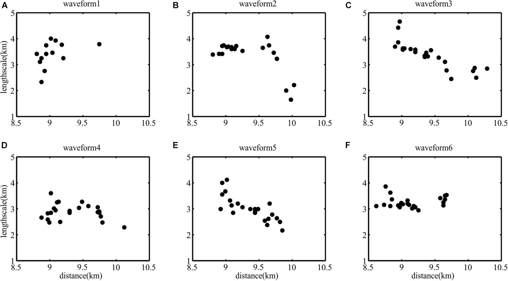
Figure 9. The change in wavelength of the six waveforms. (A–F) The black dots are observed wavelength.
Leading and Trailing Edge Slopes of Waveforms
Figure 10 shows the slopes of the leading and trailing edge of the six waveforms. In the first waveform (Figure 10A), the slope of the leading edge gradually decreased and the slope of the trailing edge had no obvious changing trend. In the second waveform (Figure 10), the slope of the leading edge decreased and the slope of the trailing edge increased. In the third waveform (Figure 10C), the slopes of the leading and trailing edge increased simultaneously. In the fourth waveform (Figure 10D) and the fifth waveform (Figure 10E), the leading edge slope was almost unchanged and the trailing edge slope increased. In the sixth waveform (Figure 10F), the leading edge slope was almost unchanged and the trailing edge slope was slightly decreased. Comparing the slopes of the six waveforms, we show that the slopes of the leading and trailing edge gradually decreased as the water depth increased.
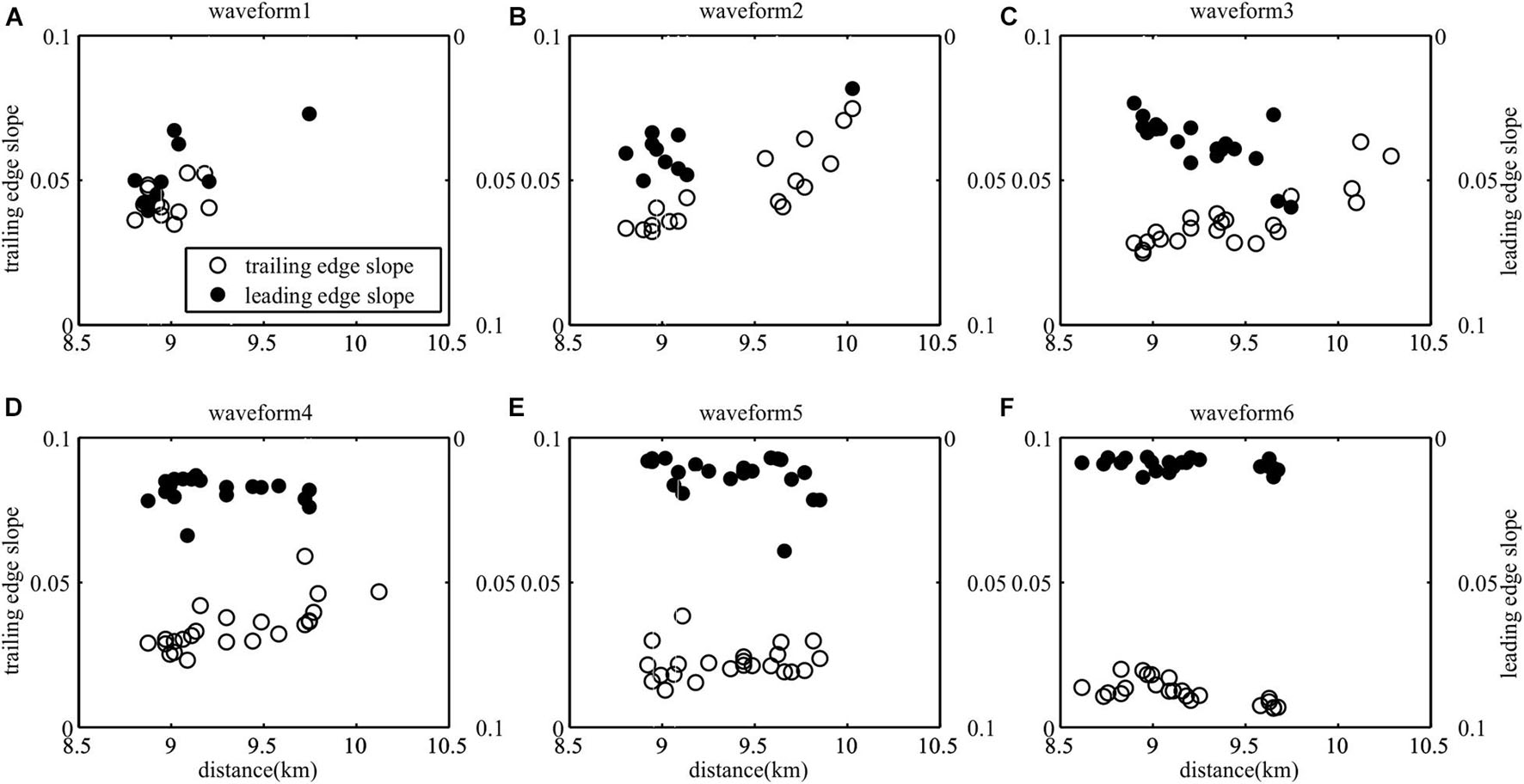
Figure 10. The changes in the slope of the leading and trailing edge of the six waveforms. (A–F) The solid black dots represent the slope of the leading edge and the slope magnitude is shown in the right-hand side. The open dots represent the slope of the trailing edge and the slope magnitude is shown in the left-hand side.
Discussion
In this study, we have observed a first-mode depression internal solitary wave shoaling onto the continental slope by utilizing prestack seismic data. The shoaling process took place in the northern South China Sea near the Dongsha Atoll. From the shape of the waveform, it can be found that the internal solitary wave was still in the early stage of shoaling and had not reversed polarity. During shoaling, the slope of the leading edge decreased and the slope of the trailing edge increased. Each waveform in Figure 6 has shown this behavior. This result is consistent with previous observations (Orr and Mignerey, 2003; Zhao et al., 2003; Bourgault et al., 2007; Shroyer et al., 2008; Fu et al., 2012) and the results of numerical simulation (Liu et al., 1998; Vlasenko and Stashchuk, 2007). In this study, we use seismic data to observe the internal solitary wave motion and use these observations to improve our understanding of their evolution.
Uniquely, seismic data allow us to visualize the evolution of thermohaline fine structure. Seismic data record an image of water column thermohaline differences (Ruddick et al., 2009) and the reflection events represent the interface of thermohaline differences. By analyzing the change of reflection events, we can understand how thermohaline structure evolves. In the seismic section, we picked six events at the different depths (Figure 6A), which represent the six waveforms of the internal solitary wave. Excluding the two near-seafloor internal solitary waves, all the waveforms leading to edges broke, as they shoaled and we hypothesize that this change is related to instability, whereby mixing reduces the local temperature and salinity gradient causing the reflection event too weaken. This is shown as seismic events breaking in the seismic section. During shoaling process, the internal solitary waves could form vortices due to the instability (Aghsaee et al., 2010) or with trapped cores (Lamb, 2002), which promote mixing in the water column and changes to the thermohaline structure. In Figure 6, the first three waveforms broke and were connected to other waveforms below. This shows that the thermohaline differences of water column weakened or disappeared under the influence of instability, so that the interface of thermohaline difference no longer existed and was eventually replaced by other reflective interfaces. All the breaks appeared in the leading edge of the internal solitary wave, which indicate that the leading edge of the internal solitary wave is more unstable during shoaling. It can be seen from Figure 6A that the depth of the internal solitary wave leading edge gradually became deeper. This is similar to the phenomenon that the depth of bottom boundary of the mixed layer at the leading edge became deeper when the internal solitary waves was shoaling, which was observed by Orr and Mignerey (2003).
Our results show that the change of waveforms is different at different depths. During shoaling, the leading edge of the waveform becomes slower and the trailing edge becomes steeper. But, the waveforms at different depths do not change simultaneously. The waveform at deeper water changes earlier than that at shallower water. These observations develop out the understanding of the causes of the shape changes of waveform. The waveform changes are believed to be driven by topography, water depth, and background flow shear (Serebryanyi, 1990; Serebryany, 1996; Vlasenko and Hutter, 2002; Orr and Mignerey, 2003). Near-seafloor waveforms are mostly affected by topography. Shroyer et al. (2008) found that the shape change of waveform was due to a greater phase velocity at the leading edge than that of the trough and trailing edge. This shear causes the leading edge to broaden, while the trailing edge remains steep. This behavior explains near-seafloor waveform changes, since the trough of waveform will first contact the seafloor and decelerate, causing the leading edge to be faster than the trough. However, the waveforms in shallow water had the same shape change without contacting the topography. We speculate that the troughs of waveforms in shallow water were decelerated by viscous forces. Due to the greater amplitude of waveforms in shallow water, the trough is more susceptible to the resistance from deep stratification. Therefore, the phase velocity of trough will gradually become smaller than that of leading edge. In addition, the amplitude is related to the degree of change in the waveform. The amplitudes of shallow waveforms are greater than those in deeper water, while deep waveforms that are constrained by topography change less with time. In summary, topography is the main inducing factor of waveform evolution, while larger amplitudes cause the waveform changes more during shoaling.
Similarly, the changes in phase velocity, amplitude, wavelength, and the leading- and trailing-edge slope are different for each waveform. During shoaling, phase velocity and amplitude increase, wavelength decreases, and the slopes of the trailing edges become larger than the leading edges. Although the phase velocities of the fourth and fifth waveforms were approximately constant, it can be seen from their trajectories in the distance-time coordinates that the non-linearity is significant. These observations indicate that non-linear effects increase as the internal solitary waves shoal and are consistent with numerical simulations results that use the Korteweg-de Vries (KdV) equations with higher-order non-linear terms (Liu et al., 1985; Liu, 1988; Grimshaw et al., 2004; Zhang and Fan, 2013). The high-order non-linear effect of the internal solitary wave observed is significant because of the large amplitudes of the waveforms. At the same time, changes in topography can also enhanced the non-linearity (Liu, 1988). The increasing non-linearity affects the internal solitary waves by increasing their amplitude and phase velocity, while decreasing their wavelengths. Shroyer et al. (2008) find a phase velocity change similar to ours. However, the initial amplitude of the wave is only 20 m, which is much smaller than the amplitude of the internal solitary wave observed and amplitude change is related to non-linearity. The amplitude of the weakly non-linear internal solitary wave increases after shoaling, but the amplitude of strongly non-linear internal wave decreases as shown by the numerical simulations (Small, 2001; Vlasenko et al., 2005) and observations (Rybak and Serebryanyi, 2011). However, the amplitude of strongly non-linear internal waves increases first at the initial stage of shoaling and then decreases rapidly. Our observations capture this process, which generally occurs in water depths of about 300 m (Small, 2001). On the other hand, Serebryany and Pao (2008) simulate a small-amplitude (14 m) internal solitary wave and show that its amplitude decreases during shoaling. Although the nonlinearity of small-amplitude internal solitary wave is weak, the shallow water depth (about 33 m) used in Serebryany and Pao’s simulation makes the nonlinearity increase, the waveform cannot adjust gradually and changes rapidly. To summarize, our observations build upon the results of numerical simulations by showing that the interplay between non-linearity and topography plays a critical role in waveform evolution during shoaling.
Conclusion
We used seismic reflection surveying to observe a first-mode depression internal solitary wave in the South China Sea near the Dongsha Atoll. The internal solitary wave was located on the continental slope and propagated from east to west toward the shelf. The maximum amplitude of the internal solitary waves is about 70 m. In order to study the evolution process of the shoaling internal solitary wave, we improved the processing scheme of seismic data. We used COGs instead of CMP gathers to image the internal solitary wave, so as to obtain 23 COG migrated sections. We are able to use these time-lapse images of internal fine structure to map the evolution of the internal solitary waves.
Seismic sections show that internal reflection structure changes during shoaling. In shallow water, the waveforms break and were connected to other waveforms. We believe that this phenomenon results from instabilities that cause the thermohaline structure of the water column to change and leads to disappearance or weakening of seismic events.
Common offset gather sections show that waveform evolution varies with depth during shoaling. Six reflection events, with different depths, reveal that topography affects deeper waveforms earlier than shallower waveforms. The degree of waveform change is related to its amplitude. Furthermore, phase velocity, amplitude, wavelength, and the leading- and trailing-edge slope also vary as a function of depth. When the internal solitary wave shoals, its amplitude and phase velocity increase, wavelength decreases, and the slope of the leading edge decreases, while the slope of the trailing edge increases. Our observations are consistent with the numerical simulations and other observations, and our adapted seismic method has furthered our understanding of the internal solitary waves. This method also has potential for studying the evolution of other physical ocean phenomena.
Data Availability Statement
The original contributions presented in the study are included in the article/supplementary material, further inquiries can be directed to the corresponding author/s.
Author Contributions
HS contributed to the conceptualization, methodology, writing, reviewing, editing, and investigation of the manuscript. YGo contributed to the investigation and writing of the manuscript. SY and YGu contributed to the investigation, data curation, and validation of the manuscript. All authors contributed to the article and approved the submitted version.
Funding
This study was supported by the National Natural Science Foundation of China (Grant Numbers 41976048 and 91128205) and the National Key R&D Program of China (2018YFC0310000).
Conflict of Interest
The authors declare that the research was conducted in the absence of any commercial or financial relationships that could be construed as a potential conflict of interest.
Publisher’s Note
All claims expressed in this article are solely those of the authors and do not necessarily represent those of their affiliated organizations, or those of the publisher, the editors and the reviewers. Any product that may be evaluated in this article, or claim that may be made by its manufacturer, is not guaranteed or endorsed by the publisher.
Acknowledgments
We would like to thank the Guangzhou Marine Geological Survey for providing 2D seismic data. The bathymetry data were provided by the General Bathymetric Chart of the Oceans (GEBCOs) (http://www.gebco.net/). The reanalysis data were provided by the CMEMS (https://resources.marine.copernicus.eu/). We would like to thank the GEBCO and the CMEMS for supporting the data in this study. We would like to thank Seismic Unix (SU) and Generic Mapping Tool (GMT) for the software support for this study. We would also like to thank the Guest Editor and reviewers for their constructive reviews and comments on the manuscript.
References
Aghsaee, P., Boegman, L., and Lamb, K. G. (2010). Breaking of shoaling internal solitary waves. J. Fluid Mech. 659, 289–317. doi: 10.1017/s002211201000248x
Alford, M. H., Peacock, T., MacKinnon, J. A., Nash, J. D., Buijsman, M. C., Centurioni, L. R., et al. (2015). The formation and fate of internal waves in the South China Sea. Nature 521, 65–69. doi: 10.1038/nature14399
Apel, J., Badiey, R. M., Chiu, C., Finette, S. S., Headrick, R., Kemp, J., et al. (1997). An overview of the 1995 SWARM shallow-water internal wave acoustic scattering experiment. IEEE J. Oceanic Engin. 22, 465–500. doi: 10.1109/48.611138
Bai, Y., Song, H., Guan, Y., and Yang, S. (2017). Estimating depth of polarity conversion of shoaling internal solitary waves in the northeastern South China Sea. Continent. Shelf Res. 143, 9–17. doi: 10.1016/j.csr.2017.05.014
Biescas, B., Armi, L., Sallarès, V., and Gràcia, E. (2010). Seismic imaging of staircase layers below the Mediterranean Undercurrent. Deep Sea Res. Part I: Oceanogr. Res. Papers 57, 1345–1353. doi: 10.1016/j.dsr.2010.07.001
Boegman, L., Ivey, G., and Imberger, J. (2005). The degeneration of internal waves in lakes with sloping topography. Limnol. Oceanogr. 50, 1620–1637. doi: 10.4319/lo.2005.50.5.1620
Boegman, L., and Stastna, M. (2019). Sediment resuspension and transport by internal solitary waves. Annu. Rev. Fluid Mech. 51, 129–154. doi: 10.1146/annurev-fluid-122316-045049
Bogucki, D. J., and Redekopp, L. G. (1999). A mechanism for sediment resuspension by internal solitary waves. Geophys. Res. Lett. 26, 1317–1320. doi: 10.1029/1999gl900234
Bourgault, D., Blokhina, M. D., Mirshak, R., and Kelley, D. E. (2007). Evolution of a shoaling internal solitary wavetrain. Geophys. Res. Lett. 34:L03601. doi: 10.1029/2006gl028462
Buffett, G. G., Biescas, B., Pelegrí, J. L., Machín, F., Sallarès, V., Carbonell, R., et al. (2009). Seismic reflection along the path of the Mediterranean Undercurrent. Continent. Shelf Res. 29, 1848–1860. doi: 10.1016/j.csr.2009.05.017
Cai, S., Gan, Z., and Long, X. (2002). Some characteristics and evolution of the internal soliton in the northern South China Sea. Chinese Sci. Bull. 47, 21–26. doi: 10.1360/02tb9004
Cai, S., and Xie, J. (2010). A propagation model for the internal solitary wavesin the northern South China Sea. J. Geophys. Res. Oceans 115:C12074. doi: 10.1029/2010JC006341
Cai, S., Xie, J., and He, J. (2012). An overview of internal solitary waves in the South China Sea. Surveys Geophys. 33, 927–943. doi: 10.1007/s10712-012-9176-0
Chen, L., Zheng, Q., Xiong, X., Yuan, Y., Xie, H., Guo, Y., et al. (2019). Dynamic and statistical features of internal solitarywaves on the continental slope in the Northern SouthChina Sea derived from mooring observations. J. Geophys. Res. Oceans 124, 4078–4097. doi: 10.1029/2018JC014843
Cheng, M.-H., and Hsu, J. R. C. (2010). Laboratory experiments on depression interfacial solitary waves over a trapezoidal obstacle with horizontal plateau. Ocean Engin. 37, 800–818. doi: 10.1016/j.oceaneng.2010.02.016
Dickinson, A., White, N. J., and Caulfield, C. P. (2020). Time-lapse acoustic imaging of mesoscale and fine-scale variability within the Faroe-Shetland Channel. J. Geophys. Res. Oceans 125:e2019JC015861. doi: 10.1029/2019JC015861
Fan, W., Song, H., Gong, Y., Sun, S., Zhang, K., Wu, D., et al. (2021). The shoaling mode-2 internal solitary waves in the Pacific coast of Central America investigated by marine seismic survey data. Continent. Shelf Res. 212:104318.
Fu, K.-H., Wang, Y.-H., St. Laurent, L., Simmons, H., and Wang, D.-P. (2012). Shoaling of large-amplitude nonlinear internal waves at The Dongsha Atoll in the northern South China Sea. Continent. Shelf Res. 37, 1–7. doi: 10.1016/j.csr.2012.01.010
Geli, L., Cosquer, E., Hobbs, R. W., Klaeschen, D., Papenberg, C., Thomas, Y., et al. (2009). High resolution seismic imaging of the ocean structure using a small volume airgun source array in the Gulf of Cadiz. Geophys. Res. Lett. 36:L00D09. doi: 10.1029/2009gl040820
Geng, M., Song, H., Guan, Y., and Bai, Y. (2019). Analyzing amplitudes of internal solitary waves in the northern South China Sea by use of seismic oceanography data. Deep Sea Research Part I: Oceanogr. Res. Papers 146, 1–10. doi: 10.1016/j.dsr.2019.02.005
Gong, Y., Song, H., Zhao, Z., Guan, Y., and Kuang, Y. (2021). On the vertical structure of internal solitary waves in the northeastern SouthChina Sea. Deep Sea Research Part I: Oceanogr. Res. Papers 173:103550. doi: 10.1016/j.dsr.2021.103550
Grimshaw, R., Pelinovsky, E., Talipova, T., and Kurkin, A. (2004). Simulation of the transformation of internal solitary waves on oceanic shelves. J. Phys. Oceanogr. 34, 2774–2791. doi: 10.1175/jpo2652.1
Grimshaw, R., Pelinovsky, E., Talipova, T., and Kurkina, O. (2010). Internal solitary waves: propagation, deformation and disintegration. Nonlinear Process. Geophys. 17, 633–649. doi: 10.5194/npg-17-633-2010
Gunn, K. L., White, N., and Caulfield, C. P. (2020). Time-lapse seismic imaging of oceanic fronts and transient lenses within South Atlantic Ocean. J. Geophys. Res. Oceans 125:e2020JC016293. doi: 10.1029/2020JC016293
Guo, C., and Chen, X. (2014). A review of internal solitary wave dynamics in the northern South China Sea. Progress Oceanogr. 121, 7–23. doi: 10.1016/j.pocean.2013.04.002
Haury, L. R., Wiebe, P. H., Orr, M. H., and Briscoe, M. G. (1983). Tidally generated high-frequency internal wave packets and their effects on plankton in Massachusetts Bay. J. Mar. Res. 41, 65–112. doi: 10.1357/002224083788223036
Holbrook, W. S., and Fer, I. (2005). Ocean internal wave spectra inferred from seismic reflection transects. Geophys. Res. Lett. 32:L15604. doi: 10.1029/2005GL023733
Holbrook, W. S., Páramo, P., Pearse, S., and Schmitt, R. W. (2003). Thermohaline fine structure in an oceanographic front from seismic reflection profiling. Science 301, 821–824. doi: 10.1126/science.1085116
Holloway, P., Pelinovsky, E. E., Talipova, T., and Barnes, B. (1997). A nonlinear model of internal tide transformation on the Australian North West Shelf. J. Phys. Oceanogr. 27, 871–896. doi: 10.1175/1520-048519970272.0.CO;2
Klymak, J. M., and Moum, J. N. (2003). Internal solitary waves of elevation advancing on a shoaling shelf. Geophys. Res. Lett. 30, OCE 3-1–OCE 1-4. doi: 10.1029/2003gl017706
Lamb, K. G. (1997). Particle transport by nonbreaking, solitary internal waves. J. Geophys. Res. Oceans 102, 18641–18660. doi: 10.1029/97jc00441
Lamb, K. G. (2002). A numerical investigation of solitary internal waves with trapped cores formed via shoaling. J. Fluid Mech. 451, 109–144. doi: 10.1017/s002211200100636x
Lamb, K. G. (2003). Shoaling solitary internal waves: on a criterion for the formation of waves with trapped cores. J. Fluid Mech. 478, 81–100. doi: 10.1017/s0022112002003269
Liao, G., Xu, X., Liang, C., Dong, C., Zhou, B., Ding, T., et al. (2014). Analysis of kinematic parameters of Internal Solitary Waves in the Northern South China Sea. Deep Sea Res. Part I: Oceanogr. Res. Papers 94, 159–172. doi: 10.1016/j.dsr.2014.10.002
Liu, A., Holbrook, K., and Apel, J. (1985). Nonliner internal wave evolution in the Sulu Sea. J. Phys. Oceanogr. 15, 1613–1624. doi: 10.1175/1520-048519850152.0.CO;2
Liu, A. K. (1988). Analysis of nonlinear internal waves in the New York Bight. J. Geophys. Res. 93:12317. doi: 10.1029/JC093iC10p12317
Liu, A. K., Chang, Y. S., Hsu, M.-K., and Liang, N. K. (1998). Evolution of nonlinear internal waves in the East and South China Seas. J. Geophys. Res. Oceans 103, 7995–8008. doi: 10.1029/97jc01918
Lynch, J. F., Ramp, S. R., Chiu, C. S., Tang, T. Y., Yang, Y. J., and Simmen, J. A. (2004). Research highlights from the Asian seas international acoustics experiment in the South China Sea. IEEE J. Oceanic Engin. 29, 1067–1074.
Magnell, B. (1976). Salt fingers observed in the Mediterranean Outflow region (34°N, 11°W) using a towed sensor. J. Phys. Oceanogr. 6, 511–523. doi: 10.1175/1520-04851976006<0511:sfoitm<2.0.co;2
Masunaga, E., Homma, H., Yamazaki, H., Fringer, O. B., Nagai, T., Kitade, Y., et al. (2015). Mixing and sediment resuspension associated with internal bores in a shallow bay. Continent. Shelf Res. 110, 85–99. doi: 10.1016/j.csr.2015.09.022
Moum, J. N., Farmer, D. M., Shroyer, E. L., Smyth, W. D., and Armi, L. (2007). Dissipative losses in nonlinear internal waves propagating across the continental shelf. J. Phys. Oceanogr. 37, 1989–1995. doi: 10.1175/jpo3091.1
Moum, J. N., Farmer, D. M., Smyth, W. D., Armi, L., and Vagle, S. (2003). Structure and generation of turbulence at interfaces strained by internal solitary waves propagating shoreward over the continental shelf. J. Phys. Oceanogr. 33, 2093–2112. doi: 10.1175/1520-04852003033<2093:SAGOTA<2.0.CO;2
Nandi, P., Holbrook, W. S., Pearse, S., Páramo, P., and Schmitt, R. W. (2004). Seismic reflection imaging of water mass boundaries in the Norwegian Sea. Geophys. Res. Lett. 31, 345–357. doi: 10.1029/2004GL021325
Orr, M. H., and Mignerey, P. C. (2003). Nonlinear internal waves in the South China Sea: Observation of the conversion of depression internal waves to elevation internal waves. J. Geophys. Res. 108:3064. doi: 10.1029/2001jc001163
Pinheiro, L. M., Song, H., Ruddick, B., Dubert, J., Ambar, I., Mustafa, K., et al. (2010). Detailed 2-D imaging of the Mediterranean outflow and meddies off W Iberia from multichannel seismic data. J. Mar. Syst. 79, 89–100. doi: 10.1016/j.jmarsys.2009.07.004
Ramp, S. R., Tang, T. Y., Duda, T. F., Lynch, J. F., Liu, A. K., Chiu, C.-S., et al. (2004). Internal solitons in the Northeastern South China SeaPart I: Sources and deep waterpropagation. IEEE J. Oceanic Engin. 29, 1157–1181. doi: 10.1109/JOE.2004.840839
Ruddick, B., Song, H., Dong, C., and Pinheiro, L. (2009). Water column seismic images as maps of temperature gradient. Oceanography 21, 192–205. doi: 10.5670/oceanog.2009.19
Rybak, S. A., and Serebryanyi, A. N. (2011). Nonlinear internal waves over the inclined bottom: observations with the use of an acoustic profiler. Acoustical Phys. 57, 77–82. doi: 10.1134/S1063771011010155
Sallarès, V., Biescas, B., Buffett, G., Carbonell, R., Dańobeitia, J. J., and Pelegrí, J. L. (2009). Relative contribution of temperature and salinity to ocean acoustic reflectivity. Geophys. Res. Lett. 36:L00D06. doi: 10.1029/2009gl040187
Sallarès, V., Mojica, J. F., Biescas, B., Klaeschen, D., and Gràcia, E. (2016). Characterization of the submesoscale energy cascade in the Alboran Sea thermocline from spectral analysis of high-resolution MCS data. Geophys. Res. Lett. 43, 6461–6468. doi: 10.1002/2016GL069782
Scotti, A., and Pineda, J. (2004). Observation of very large and steep internal waves of elevation near the Massachusetts coast. Geophys. Res. Lett. 31:L22307. doi: 10.1029/2004gl021052
Serebryany, A. N. (1996). Steepening of the leading and back faces of solitary internal waves depressions and its connections with tidal currents. Dynamics Atmos. Oceans 23, 2075–2091. doi: 10.1016/0377-0265(95)00427-0
Serebryany, A. N., and Pao, H. P. (2008). Transition of a nonlinear internal wave through an overturning point on a shelf. Doklady Earth Sci. 420, 714–718. doi: 10.1134/S1028334X08040430
Serebryanyi, A. N. (1990). Internal wave effects of nonlinearity at the shelf. Izvestia Akademii nauk SSSR. Fizika Atmosfery i Okeana 26, 285–293.
Sheen, K. L., White, N. J., Caulfield, C. P., and Hobbs, R. W. (2012). Seismic imaging of a large horizontal vortex at abyssal depths beneath the Sub-Antarctic Front. Nature Geosci. 5, 542–546. doi: 10.1038/ngeo1502
Shroyer, E. L., Moum, J. N., and Nash, J. D. (2008). Observations of polarity reversal in shoaling nonlinear internal waves. J. Phys. Oceanogr. 39, 691–701. doi: 10.1175/2008JPO3953.1
Small, J. (2001). A nonlinear model of the shoaling and refraction of internal solitary waves in the ocean. Part I: development of the model and investigations of the shoaling effect. J. Phys. Oceanogr. 31, 3163–3183. doi: 10.1175/1520-04852001031<3163:ANMOTS<2.0.CO;2
Tang, Q., Gulick, S. P. S., Sun, J., Sun, L., and Jing, Z. (2020). Submesoscale features and turbulent mixing of an oblique anticyclonic eddy in the Gulf of Alaska investigated by marine seismic survey data. J. Geophys. Res. Oceans 125:e2019JC015393. doi: 10.1029/2019jc015393
Tang, Q., Hobbs, R., Wang, D., Sun, L., Zheng, C., Li, J., et al. (2015). Marine seismic observation of internal solitary wave packets in the northeast South China Sea. J. Geophys. Res. Oceans 120, 8487–8503. doi: 10.1002/2015jc011362
Tsuji, T., Noguchi, T., Niino, H., Matsuoka, T., Nakamura, Y., Tokuyama, H., et al. (2005). Two-dimensional mapping of fine structures in the Kuroshio Current using seismic reflection data. Geophys. Res. Lett. 32:L14609. doi: 10.1029/2005gl023095
Vlasenko, V., Brandt, P., and Rubino, A. (2000). Structure of large-amplitude internal solitary waves. J. Phys. Oceanogr. 30, 2172–2185. doi: 10.1175/1520-04852000030<2172:SOLAIS<2.0.CO;2
Vlasenko, V., and Hutter, K. (2002). Numerical experiments on the breaking of solitary internal waves over a slope–shelf topography. J. Phys. Oceanogr. 32, 1779–1793. doi: 10.1175/1520-04852002032<1779:NEOTBO<2.0.CO;2
Vlasenko, V., Ostrovsky, L., and Hutter, K. (2005). Adiabatic behavior of strongly nonlinear internal solitary waves in slope shelf areas. J. Geophys. Res. 110:C04006. doi: 10.1029/2004JC002705
Vlasenko, V., and Stashchuk, N. (2007). Three-dimensional shoaling of large-amplitude internal waves. J. Geophys. Res. 112:C11018. doi: 10.1029/2007jc004107
Wunsch, C., and Ferrari, R. (2004). Vertical mixing, energy, and the general circulation of the oceans. Annu. Rev. Fluid Mech. 36, 281–314. doi: 10.1146/annurev.fluid.36.050802.122121
Yilmaz, Ö (2001). Seismic data analysis: Processing, inversion, and interpretation of seismic data. Soc. Explorat. Geophys. 10:2092. doi: 10.1190/1.9781560801580
Zhang, S.-W., and Fan, Z.-S. (2013). Effects of high-order nonlinearity and rotation on the fission of internal solitary waves in the South China Sea. J. Hydrodyn. 25, 226–235. doi: 10.1016/s1001-6058(13)60357-1
Zhao, Z., Klemas, V., Zheng, Q., Li, X. and Yan, X. H. (2003). Satellite observation of internal solitary waves converting polarity. Geophys. Res. Lett. 30:1988. doi: 10.1029/2003gl018286
Zhao, Z., Klemas, V., Zheng, Q., and Yan, X.-H. (2004). Remote sensing evidence for baroclinic tide origin of internal solitary waves in the northeastern South China Sea. Geophys. Res. Lett. 31:L06302. doi: 10.1029/2003gl019077
Zheng, Q., Susanto, R. D., Ho, C.-R., Song, Y. T., and Xu, Q. (2007). Statistical and dynamical analyses of generation mechanisms of solitary internal waves in the northern South China Sea. J. Geophys. Res. 112:C03021. doi: 10.1029/2006jc003551
Keywords: internal fine structure, internal solitary wave, shoaling, northern South China Sea, seismic oceanography
Citation: Song H, Gong Y, Yang S and Guan Y (2021) Observations of Internal Structure Changes in Shoaling Internal Solitary Waves Based on Seismic Oceanography Method. Front. Mar. Sci. 8:733959. doi: 10.3389/fmars.2021.733959
Received: 30 June 2021; Accepted: 13 October 2021;
Published: 11 November 2021.
Edited by:
Kathy Gunn, University of Miami, United StatesReviewed by:
Andrey Serebryany, P. P. Shirshov Institute of Oceanology, Russian Academy of Sciences (RAS), RussiaShuqun Cai, South China Sea Institute of Oceanology, Chinese Academy of Sciences (CAS), China
Copyright © 2021 Song, Gong, Yang and Guan. This is an open-access article distributed under the terms of the Creative Commons Attribution License (CC BY). The use, distribution or reproduction in other forums is permitted, provided the original author(s) and the copyright owner(s) are credited and that the original publication in this journal is cited, in accordance with accepted academic practice. No use, distribution or reproduction is permitted which does not comply with these terms.
*Correspondence: Haibin Song, aGJzb25nQHRvbmdqaS5lZHUuY24=; Yi Gong, Y3FkYmMwMjRAMTI2LmNvbQ==