Overexploitation, Recovery, and Warming of the Barents Sea Ecosystem During 1950–2013

The Barents Sea (BS) is a high-latitude shelf ecosystem with important fisheries, high and historically variable harvesting pressure, and ongoing high variability in climatic conditions. To quantify carbon flow pathways and assess if changes in harvesting intensity and climate variability have affected the BS ecosystem, we modeled the ecosystem for the period 1950–2013 using a highly trophically resolved mass-balanced food web model (Ecopath with Ecosim). Ecosim models were fitted to time series of biomasses and catches, and were forced by environmental variables and fisheries mortality. The effects on ecosystem dynamics by the drivers fishing mortality, primary production proxies related to open-water area and capelin-larvae mortality proxy, were evaluated. During the period 1970–1990, the ecosystem was in a phase of overexploitation with low top-predators’ biomasses and some trophic cascade effects and increases in prey stocks. Despite heavy exploitation of some groups, the basic ecosystem structure seems to have been preserved. After 1990, when the harvesting pressure was relaxed, most exploited boreal groups recovered with increased biomass, well-captured by the fitted Ecosim model. These biomass increases were likely driven by an increase in primary production resulting from warming and a decrease in ice-coverage. During the warm period that started about 1995, some unexploited Arctic groups decreased whereas krill and jellyfish groups increased. Only the latter trend was successfully predicted by the Ecosim model. The krill flow pathway was identified as especially important as it supplied both medium and high trophic level compartments, and this pathway became even more important after ca. 2000. The modeling results revealed complex interplay between fishery and variability of lower trophic level groups that differs between the boreal and arctic functional groups and has importance for ecosystem management.

Introduction

Fisheries and climate have been emphasized as major drivers of energy flows in large marine ecosystems (LMEs) (Araujo and Bundy, 2012; Link et al., 2012), and understanding how these drivers interacts and shapes ecosystems is a major challenge and essential to manage these ecosystems. It is important to investigate how these drivers interplay in high-latitude ecosystems, such as the Barents Sea. The Barents Sea (BS) is intensely exploited and profoundly impacted by climate variability. It is characterized by a strong temperature gradient with boreal and sub-arctic conditions in the southwest and high-arctic conditions in the northeast (Loeng, 1991; Smedsrud et al., 2010), and advected heat, nutrients, and biota, along with seasonally migrating fish, seabirds, and mammals strongly impact ecosystem structure and production (Hunt et al., 2013). The trophic structure of the BS ecosystem is similar to other northern high latitude shelf ecosystems (Gaichas et al., 2009; Eriksen et al., 2017).

Fisheries has been a major direct driver of marine ecosystems the past century, affecting structure, function, and diversity (Jackson, 2001; Halpern et al., 2008). The fisheries within the BS have since the 1950s been targeting mainly large gadoid fishes, such as Atlantic cod (Gadus morhua), haddock (Melanogrammus aeglefinus) and saithe (Pollachius virens) and other demersal fishes, such as Greenland halibut (Reinhardtius hippoglossoides) and redfishes (Sebastes mentella and Sebastes norvegicus), the small pelagic fish species capelin (Mallotus villosus) and polar cod (Boreogadus saida), and northern shrimp (Pandalus borealis) (Gjøsæter, 1998; Nakken, 1998; Hop and Gjøsæter, 2013; Haug et al., 2017). Juvenile Atlantic herring (Clupea harengus) was fished within the area from 1950 to 1971 (Toresen and Østvedt, 2000). Some marine mammals were also heavily exploited up until their protection, such as walrus (Odobenus rosmarus) (protected in 1952), polar bear (protected in 1973), and some large baleen whales (Nakken, 1998; Weslawski et al., 2000). After ca 1970, the only mammals harvested in large scale have been minke whales and harp seals (Nakken, 1998).

Climate variability may affect marine ecosystems through effects on primary and secondary production, fish recruitment variability, growth and shifts of populations distribution range (Nilssen et al., 1994; Ottersen and Loeng, 2000; Fossheim et al., 2015). In the BS, a period of warm climate between 1920 and 1960 was followed by a cold period from ca. 1960 to 1980 and then by a period of warming after the 1980s (Loeng and Drinkwater, 2007). Temperature variability has affected recruitment to the commercial fish stocks Norwegian spring spawning herring, Northeast Arctic cod and haddock with larger year-classes produced in warmer years (Ottersen and Loeng, 2000; Sundby, 2000). The warming of the BS ecosystem since the early 1980s (Johannesen et al., 2012) has resulted in northwards shift in distribution and increasing abundance for boreal fish species and a decrease for arctic fish species (Eriksen et al., 2011; Kortsch et al., 2015) and an increased importance of benthic invertebrate species with affinity for warmer waters (Jørgensen et al., 2019). After 1980, temporal fluctuations in population sizes have been observed at several trophic levels, e.g., krill, northern shrimp, capelin, and seabirds (Johannesen et al., 2012; Fauchald et al., 2015; Gjøsæter et al., 2015). Relationships and energetics of major stocks of top-predators, such as Northeast Arctic cod, minke whales, and harp seals have also changed (Bogstad et al., 2015; Fauchald et al., 2015).

The change in climatic conditions call for an effort to use and integrate available information to understand the underlying drivers for the ecosystem changes, and ecosystem modeling is a common tool to synthesize quantitative information into a coherent system. This is particularly important in species-rich systems with complex (e.g., with considerable advection and migration) pathways for impact where statistical modeling may struggle. Previously published food web models of the BS and Norwegian Sea have been fish-centered with relatively few lower trophic level groups and benthic invertebrate groups (Blanchard et al., 2002; Dommasnes et al., 2002; Hansen et al., 2016; Skaret and Pitcher, 2016; Bentley et al., 2017). Arctic and sub-Arctic ecosystems, however, are well-known for the strong role of seafloor communities in regulating carbon cycling pathways (Kędra and Grebmeier, 2021). Based on a dynamic mass-balance model (Ecopath with Ecosim-EwE) and future warming scenarios for the Norwegian and the BS, Bentley et al. (2017) suggested that the biomasses of widely migrating pelagic species, such as mackerel and blue whiting, are expected to increase with future rising ocean temperature. There is some evidence that effects of climate variability on the ecosystem in the BS is largely through bottom-up effects on lower trophic level groups that propagate to higher trophic level groups (Johannesen et al., 2012; Dalpadado et al., 2014, 2020).

Fisheries and climate change may act synergistically with each other and/or with other anthropogenic disturbances (Fogarty et al., 2008; Hsieh et al., 2008). Exploited populations may be less resilient to climate variability than unexploited populations due to more truncated age structure and diversity in life history traits (Fogarty et al., 2008; Hsieh et al., 2008). A better understanding of how exploitation and climate variability influence the ecosystem dynamics will support management of marine resources.

Aggregating species into trophic groups may mask complex species interactions and influence calculations associated with food webs and interspecific competition (Thompson and Townsend, 2000). Therefore, to analyze trophic interactions and impacts of harvesting and climate variability in this study, we parametrized an Ecopath food web model for the BS with both Atlantic boreal and Arctic groups, and with a high resolution of lower trophic level groups. This model was evaluated and fitted to time-series of biomasses and fisheries data (catches, fishing mortalities). The main objectives of this study were to evaluate how changes in exploitation and climate have affected ecosystem structure, metrics, and properties of the BS ecosystem during the period 1950–2013. The specific aims were to; (i) quantify carbon flow pathways and production by ecological compartments, (ii) investigate whether past exploitation have reduced biomass and productivity of functional groups and led to trophic-cascade-related effects, and (iii) assess if climate variability affected the ecosystem productivity and if boreal and arctic groups were affected differently.

We will use available updated information on trophic linkages to parametrize a highly resolved Ecopath with Ecosim food web model in the time-period 1950–2013. The model was fitted and calibrated to group-specific time-series of biomasses and catches and forced by environmental drivers, such as fishing mortality, primary production, and capelin larvae mortality proxies. The effects of exploitation and climate variability was evaluated by the ecosystem metrics and properties produced by this model. We discuss how our findings may support an ecosystem based management of the BS.

Materials and Methods

Study Area, Environment, and Data Collection

The BS is a high latitude LME, covering an area of 2.01 million km² (Skjoldal and Mundy, 2013), extending from the Norwegian Sea and eastwards to Novaya Zemlja and northwards from the coast of Norway and Russia to about 80°N (Drinkwater, 2011; Figure 1).

FIGURE 1

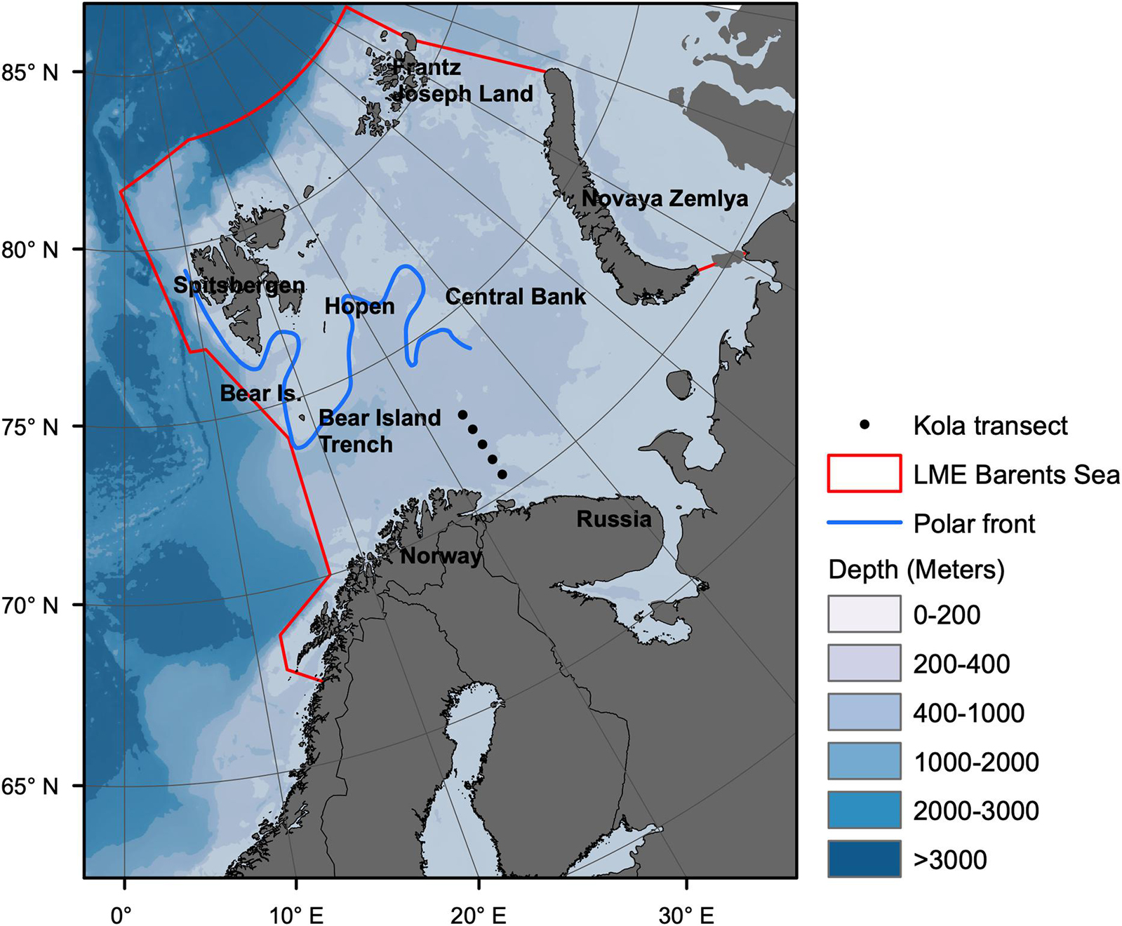
Figure 1. Map of Barents Sea large marine ecosystem. Borders of the ecosystem are shown by red lines Based on (https://www.pame.is/projects/ecosystem-approach/arctic-large-marine-ecosystems-lme-s). The Kola transect stations 3–7 for hydrographic monitoring are shown as black dots. Location of the polar front is shown by blue line.

Water circulation and currents in the BS are strongly influenced by the bottom topography. The shallowest areas are found around Spitsbergen Bank and in the southeastern part with depths <50 m (Loeng, 1991). The deepest area (deeper than 400 m) is found in the western part where the main influx of relatively warm Atlantic (T > 2°C) and Coastal (T > 3°C) waters enters the BS (Loeng and Drinkwater, 2007). Cold Arctic (T < 0°C) water penetrates the system from the east and north (Hunt et al., 2013). The Polar Front is a transition zone between the warmer boreal southern part and the colder Arctic northern part (Figure 1; Fossheim et al., 2015). During winter, the edge of the seasonal ice cover was normally found just north of the Polar Front (Smedsrud et al., 2013). The ice cover varies both seasonally and inter-annually (Wassmann et al., 2006a; Smedsrud et al., 2013), with maximum coverage typically in March-April and the minimum coverage in August-September (Drinkwater, 2011). The climatic gradient within the BS is reflected in the distribution of organisms (Andriyashev and Chernova, 1995; Jørgensen et al., 2015; Renaud et al., 2018). Boreal fish species have generally expanded northwards at the expense of arctic species during the recent warm period (Fossheim et al., 2015).

Data to parametrize, drive and evaluate the Ecopath and Ecosim models were collected from literature and published data sources from the BS (Supplementary Appendices 2, 4). In cases were data from BS were not available, data from other similar areas were used (Supplementary Appendix 2).

Model Description

The Ecopath model tracks Carbon as the mass unit to reflect the varying organic carbon content of functional groups. Organic carbon has a much stronger relationship to energy than wet mass (Salonen et al., 1976) and carbon is commonly used as unit in Ecopath models with emphasis on lower trophic levels (Tomczak et al., 2009).

The Ecopath model consist of two master equations (Christensen et al., 2005). The first equation describes how production for a FG i is split into various components

$$P_i=Y_i+B_{i}M{2}_i+E_i+B{A}_i+P_i(1-EE)(1)$$

Equation 1 can be written as;

$$B_i{\left(\frac{P}{B}\right)}_i=\sum _{j=1}^n{B}_j{\left(\frac{Q}{B}\right)}_j{\mathit{DC}}_{\mathrm{ji}}+Y_i+E_i+{\mathit{BA}}_i+B_i{\left(\frac{P}{B}\right)}_i\left(1-{\mathit{EE}}_i\right)(2)$$

where P_i is the production of group i, Y_i is the catch of group i, M2_i is the predation mortality rate on groups i, B_i is the biomass (g C m^–2), (P/B)_i is the production/biomass ratio of group i, (Q/B)_j is the consumption/biomass ratio of predator j, DC_ji is the proportion of prey group i in the diet of predator j, Y_i is the catch, E_i is net emigration, BA_i is the biomass accumulation and B_i(P/B)_i(1 - EE_i) is other mortality of group i. EE_i is the ecotrophic efficiency describing the proportion of production of a group that is consumed within the model.

Within each FG i, energy balance is ensured using the equation

$$\begin{array}{c}\mathrm{Consumption}=\mathrm{production}+\mathrm{respiration}\hfill \\ +\mathrm{unassimilated}\mathrm{food}\hfill \end{array}(3)$$

The BS Ecopath model for year 2000 comprises 108 functional groups (FG) of which 19 groups were multi-stanza groups (Table 1 and Supplementary Appendices 1–3). Multi-stanza groups contain a set of biomass groups representing life history stages or stanzas for species that have complex trophic ontogeny (Heymans et al., 2016). Species were grouped in FGs based on their similarities in diet composition, production/biomass ratio (P/B) and consumption/biomass ratio (Q/B), predators and predatory mortalities.

TABLE 1

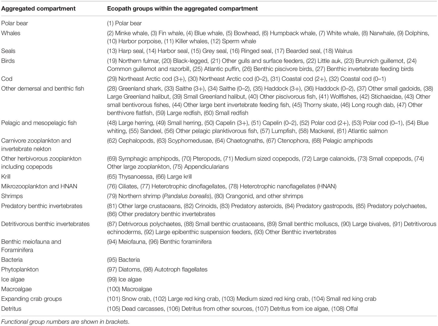
Table 1. Overview of groups for which output values from Ecopath were aggregated into major compartments.

Input Data to Ecopath Models

The Ecopath model for 1950 was based on an Ecopath model for year 2000 but with biomass, fisheries, P/B and Q/B-values specific for year 1950. Less information regarding many ecological groups was available for the period around 1950 and we chose year 2000 to represent a presumably similar year as 1950 with regard to temperature, and for balancing an annual average year 2000 Ecopath model. The average temperature in the Kola-section in 2000 was similar to 1950 (4.6°C vs. ca. 4.7°C) (Dippner and Ottersen, 2001; Supplementary Figure 1). The water temperature time-series from 1951 to 2013 (average from 0 to 200 m depth, st. 3–7) from the Kola section (70°30′N to 72°30′N along 33°30′E) [source: Knipovich Polar Research Institute of Marine Fisheries and Oceanography (PINRO)]¹ (Figure 1) has been considered as a good indicator for the temperature variability in the BS (Stige et al., 2010).

The annual average Ecopath model representing year 2000 was parameterized by the best available literature data (Supplementary Appendix 2). Data for biomass, catches, diet composition, production/biomass, consumption/biomass, and assimilation efficiency, were mainly derived from the BS. For data-rich groups, such as commercially exploited fish, northern shrimp and top-predators, where abundance or biomass are regularly monitored, biomass and catch time-series could be calculated (Supplementary Appendix 4 Part A,B). For less surveyed groups, diet composition and other parameters were averaged on longer time-periods. Catch data were retrieved from official statistics (ICES) and time-series from publications. After parametrizing and balancing the year 2000 model, it was modified to a year 1950-model by entering year-specific values for biomasses and catches for groups with known data and the 1950-model was balanced (Supplementary Appendix 2). The modeled and observed biomass and catch trajectories of Ecosim based on the 1950 Ecopath model as “starting point” were compared to evaluate the parametrization.

P/B was often calculated from data on total annual mortality rate (Z, yr^–1) as P/B = Z (Heymans et al., 2016). Diet composition data for upper trophic levels (TL ≥ 3) FGs (fish, mammals, and birds), were mostly based on stomach analysis. When several data sets of diet composition were available for a functional group, diet proportions were averaged to provide initial input values (Supplementary Appendix 4 Part C). Diet compositions were converted from wet mass units in the original data sets to carbon mass using group specific carbon/wet mass factors (C/WW) (Supplementary Appendix 2).

To assess uncertainty in the input values for biomass, P/B, Q/B, diet and catch, pedigree scores were allocated to each input value using the system for pedigree indices integrated into EwE (Supplementary Appendix 1 Tables 1-3, 1-4). Pedigree indices are uncertainty scores assessed by the modeler for each input value in Ecopath and were based on either measured uncertainty or assessed from the type of data and the source of the input value. A 95% confidence interval is associated with each index value.

Balancing Ecopath Models

The BS ecosystem is a well-studied and ecological knowledge has accumulated. The Ecopath modeling allows us to evaluate the compatibility of the input data and identify uncertainty in the input data and in the model output because if the Ecopath model is unbalanced, the input data are not compatible. Before and after balancing the Ecopath models, the pre-balance procedure (PREBAL) was used to check if input values were within accepted ecological constraints (Link, 2010; Supplementary Appendix 4 Part D). Biomass, Q/B and P/B decreased with increasing TL, except for some mammals and bird groups that have high Q/B-values.

Balancing the Ecopath models was done manually by checking that EE ≤1 for the mammal, bird and fish groups where biomass input data were available. For groups where the biomass was estimated by the Ecopath model from consumption by its predators and catches, it was checked that biomass values were within the range reported in the literature (Supplementary Appendix 2). Gross efficiencies (P/Q) were checked to be in accordance to the literature, and it was checked that respiration/assimilation were <1. The models were constructed using version 6.6.3.16996 of EwE.² To simplify presentation of model results, some output values were presented for aggregated compartments (Table 1).

Dynamic Simulations Using Ecosim

A dynamic Ecosim model was constructed based on the 1950 Ecopath model. In Ecosim, the biomass growth rate of functional group i is expressed as

$$\frac{{\mathit{dB}}_i}{\mathit{dt}}={\left(P/Q\right)}_i\sum Q_{\mathit{ji}}-\sum Q_{\mathit{ij}}+I_i-(M_i+F_i+e_i)B_i(4)$$

Where (P/Q)_i is the gross efficiency, M_i is the natural mortality not caused by predation, F_i is the fishing mortality rate, I_i is the immigration rate, e_i is the emigration rate and B_i is the biomass (Coll et al., 2009). The consumption rates in Ecosim (Q_ji) are based on the “foraging arena theory” where the biomass of prey i is divided into a non-vulnerable and a fraction that is vulnerable to predation (Walters and Korman, 1999) and vulnerabilities (v_ij) express the maximum increase in predation mortality when predator abundance is high. Vulnerabilities (v_ij) and a number of other parameters affect consumption rate (Q_ij) of a group i preyed by a predator j (Christensen et al., 2005).

$$Q_{ij}=\frac{a_{ij}.v_{ij}.B_i.P_j.T_i.T_j.S_{ij}.M_{ij}/D_j}{v_{ij}+T_i+M_{ij}+a_{ij}.M_{ij}.P_j.S_{ij}.T_j/D_j}(5)$$

Where a_ij is the effective search rate on a prey j, T_i is the relative feeding time of prey, T_j is the relative feeding time of the predator, S_ij is a seasonal or long-term forcing function, M_ij is a median function and D_j represent effects of handling time.

Low vulnerabilities close to 1.0 are associated with a low increase in predation mortality when predator biomass increase and vice versa for high vulnerabilities. In Ecosim, the additional parameters that limit the consumption rates (Eq. 5) (Christensen et al., 2005) were set to default values during the simulations.

Ecosim Time-Series Fitting, Model Calibration, and Cross-Validation

In fitting and calibrating ecological models, there is a potential risk of overfitting models (Wenger and Olden, 2012). To evaluate Ecosim models, the model fit to time-series data, model behavior and the model’s ability to predict a part of the time-series not used in the fitting (cross-validation) were considered. We performed a cross-validation where the available time-series were split into a part (ca. 75%) used for model fitting (1950–1996) and a part used for testing the predictability of the models (1997–2013) (Bergmeir and Benítez, 2012; Wenger and Olden, 2012). A model’s ability to predict for a time-period not used in fitting informs about its transferability. Transferability has been emphasized as an important aspect of model evaluation and cross-validation has been suggested as a method to assess transferability and reduce risk of overfitting (Wenger and Olden, 2012).

Ecosim models were fitted to time-series for the period 1950–1996 and calibrated by estimating predator-prey vulnerabilities (v_ij). The number of vulnerabilities that can be estimated is equal to the number of independent time-series minus one (Scott et al., 2016). A common approach in Ecosim calibration/fitting to time-series has been to fit a spline-function which is considered a proxy for primary production, and then relate this spline function to environmental proxies, such as NAO-indices and water temperature (Skaret and Pitcher, 2016; Bentley et al., 2017). However, we found it more appropriate to include a well-documented relationship for PPR as an environmental driver. Before the Ecosim model was fitted to time-series, the time-series were categorized into “forcing” (forcing the model to time-series values), “absolute” (absolute values were used), “relative” (relative values, such as catch per unit effort were used). A total of 84 time-series were used as input in the time-series fitting, including time-series on absolute biomass (n = 32), relative biomass (n = 15), forced biomass (n = 3), forced catch (n = 9), catches (n = 9), fishing mortality (n = 14), harvesting effort (n = 2). This amounts to a total of 56 time-series on absolute and relative biomasses and catches that were used to calculate sum of squares and a potential maximum of 55 vulnerabilities could be fitted. A lognormal error distribution was assumed minimizing the sum of squares of log observed values from log modeled values (Christensen et al., 2005). There were equal weights of each time-series, thus the absolute scale of time-series values did not influence the sum of squares. The mesozooplankton biomass time-serie mainly comprising the FGs medium sized copepods, large calanoids, and small copepods, was not used in the fitting but was compared to the model output of the sum of biomass of its FGs. In addition, various environmental time-series were used as driving forces for the model (Supplementary Appendix 4 Part A,B).

An automatic step-wise fitting procedure was used to calibrate the Ecosim-model to observed time-series for biomass fishing mortalities and catches (Scott et al., 2016). This procedure statistically estimates how much fishery time-series, trophic interactions (predator-prey vulnerabilities) and environmental time-series contribute to model fit. The stepwise fitting procedure constructs a series of model permutations with increasing number of estimated vulnerabilities (v) and determines which combination of vulnerabilities gives the best statistical fit using sums of squares (SS) and Akaike’s Information Criterion modified for small samples (AICc) as criteria to select the most parsimonious model (Akaike, 1974; Kletting and Glatting, 2009).

The fitting and model evaluation procedure include several steps. (i) The sensitivities of SS for the chosen number of model vulnerabilities for each predator-prey interaction or predator were calculated and FGs with the highest sensitivities were selected. (ii) It was searched iteratively for values of vulnerabilities among the selected vulnerabilities to minimize the SS for the period 1950–1996. (iii) Plots of model-fitted and observed time-series of biomasses and catches and SS for separate FG were visually inspected to evaluate model fit to observation data and assess if the model behavior was credible (Mackinson, 2014; Heymans et al., 2016). To assess the effects of fisheries, environmental drivers and trophic factors (vulnerabilities), alternative models were tested. Alternative models were fitted without fishery data (baseline models with no catch or fishing mortality), with fisheries data and environmental forcing time-series and with and without estimating vulnerabilities resulting in a SS and an AICc-value per model. (iv) In the model prediction runs for the period 1997–2013, the predictability of models was assessed by calculating the SS for model output biomass and catches and the corresponding observed data.

To assess the effect of climatically forced phytoplankton primary production (PPR), in Ecosim, two alternative forcing time-series were tested; a constant PPR-proxy and a PPR-proxy based on the relationship between phytoplankton primary production and open-water area (Supplementary Appendix 4 Part A). A capelin larvae mortality proxy was calculated based on the relationship between biomass of small herring and capelin larvae mortality rate (Supplementary Appendix 4 Part A) and the proxy was used to force mortality rates of capelin (0–2) in model fitting.

The possible effects of change in ice-coverage on ice-algae primary production were tested by modifying model M10 by forcing ice-algae biomass directly by the ice-cover in a model M11 run (Supplementary Appendix 4 Part A) for the period 1950–2013, and the results from model M11 were compared to model M10 without forcing of the ice-algae. To test if the invasive red king crab and the expanding snow crab may have affected the ecosystem, models with snow-crab and red king crab groups were run for the period 2000–2013 (Supplementary Appendix 4 Part E). The year 2000 model with 26 estimated vulnerabilities from model M10 was run with (model M12) and without (model M13) forcing by observed crab biomass time-series (Supplementary appendix 4 Part A), and the output biomasses from the Ecosim models were compared.

Monte Carlo Simulations and Model Evaluation

For model(s) considered to have most support assessed by the stepwise fitting for the period 1950–1996, inspection of model behavior and test of predictability for the period 1997–2013, Monte Carlos simulations (MCS) were run to assess uncertainty in output values from Ecopath and Ecosim. In the MCS, input values were randomly sampled from uniform distributions with the width of the distributions corresponding to pedigree-specified input uncertainty level for biomasses, P/B and Q/B values (Supplementary Appendices 1, 2), and the MCS routine included 200 successful trials with balanced models. Each trial had up to 10,000 runs where Ecopath input parameter values were drawn and it was tested if the resulting Ecopath model was balanced. To evaluate uncertainty and compare model outputs with observed data, the 0.025 and 0.975 percentiles of the MCS outputs were calculated.

To evaluate the model fit, Taylor diagrams were used to simultaneously visualize the correlation (Pearson) between observed and modeled time-series, the root-mean-square difference (RMS) and the ratio of the standard deviations of the simulated and the observed time-series (RSD) (Taylor, 2001).

Ecosystem Indicators

It has been advised to use a variety of indicators at the community level to detect ecosystem impacts of fishing (Fulton et al., 2005). The indicators should include groups directly impacted by the fishery, charismatic groups with slow dynamics and response (e.g., mammals) and groups with fast dynamics and response (e.g., zooplankton). We calculated several indicators to assess effects of harvesting and the ecosystem states and changes during the time period 1950–2013 (Table 2).

TABLE 2

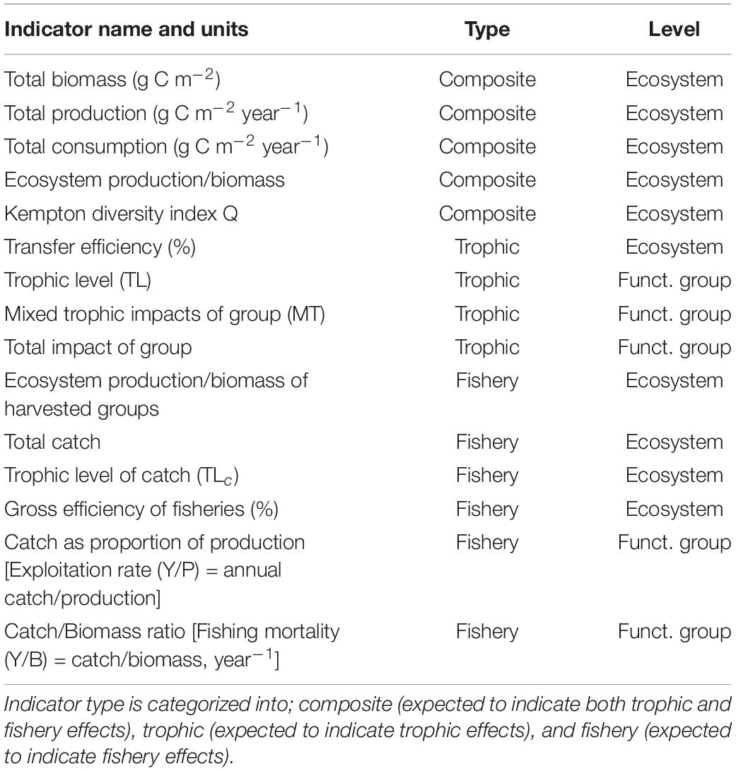
Table 2. List of indicators at ecosystem and functional group level.

The trophic levels of catches and ecosystem biomass may be affected by fisheries and have been used as indicator for ecosystem changes, with both expected to decrease in response to size-selective exploitation (Branch et al., 2010). Ecopath calculates trophic level (TL) of the FGs, catches and various indices based on TL. The TL_j of each predator group j was calculated using the equation:

$$T{L}_j=1+\sum _{i=1}^{n}D{C}_{ij}T{L}_i\mathit{\hspace{1em}}(6)$$

Where DC_ij is the proportion of prey i in the diet of predator j and TL_i is the trophic level of group i. In Ecopath it is assumed that all the detritus groups have trophic level 1.

Trophic transfer efficiency calculated for a given trophic level is the ratio between the sum of exports plus the flow that is transferred from one trophic level to the next and the throughput on the trophic level (Christensen and Walters, 2004).

The sum of all direct and indirect effects of a FG on the food web were quantified applying mixed trophic impacts (Heymans et al., 2014). The mixed trophic impact m_ij of a group is the product of all net impacts for all possible pathways that link groups i and j (Christensen and Pauly, 1992; Libralato et al., 2006). The total impact of each ecological group e_i is calculated as

$$e_i=\sqrt{\sum _{j\ne i}^n{m}_{ij}^2}(7)$$

A modified variant of the Kempton diversity index (Kempton Q) has been developed and implemented in EwE to measure the effects of fishing or climate on species in whole ecosystem models. Kempton Q express biomass diversity of groups with TL ≥3 and was expected to decrease with ecosystem degradation (Ainsworth and Pitcher, 2006; Steenbeek et al., 2018).

Production of each functional group over the modeled time period was calculated and total ecosystem production/biomass ratio and P/B-ratio of non-primary producers FGs and of harvested FGs were calculated. These P/B-ratios were expected to increase if high exploitation intensity decreases the proportion of long-lived exploited FGs biomass to total ecosystem biomass. The fishing mortality rate (F, year^–1) for each exploited FG on a biomass basis (F = Y/B) was calculated as the ratio of annual catch yield (Y, g C m^–2 year^–1) and biomass (g C m^–2). Fishing mortality is strongly positively related to fishing effort. The ratio of annual catch yield to annual production (Y/P = catch yield/production) will be used an indicator for intensity of exploitation of exploited groups (Mertz and Myers, 1998). The optimal FG specific exploitation rate (Y/P) that correspond to maximum sustainable yield from single stock considerations have been assessed to be about or slightly below 0.5, i.e., approximately equal fishing and natural mortality rate (Patterson, 1992; Zhou et al., 2012).

Results

Model Parametrization, Evaluation, and Fitting of Ecosim Models

Initially in the balancing procedure, production of pelagic fish prey was less than consumption (i.e., EE > 1.0) in the year 2000 and 1950 models, and the biomass values for capelin and polar cod had to be increased relative to initial values (Supplementary Appendices 2, 4 Part F) to balance the models. In the balancing of the 1950-model, biomass values and total mortality rates for the small herring, capelin and polar cod were increased relative to the initial values to balance the need for prey (Supplementary Appendix 4 Part F). Most FGs except for the mammal and bird groups in the balanced year 2000 and 1950-models had relatively high EE’s indicating that most of the production from most groups were consumed by groups within the model.

All models fitted to time-series for the 1950–1996 time-period without estimated vulnerabilities (M1, M3, M5, M7, and M9) had higher AICc and poorer fit than the corresponding models with estimated vulnerabilities (M2, M4, M6, M8, and M10) (Table 3). Among the former models, the baseline model M2 fitted without fisheries data had much higher AICc than the models (M4, M6, M8 and M10) fitted to fisheries data and with estimated vulnerabilities (Table 3). The two models (M8 and M10) with estimated vulnerabilities and forced by the capelin (0–2) mortality proxy had lower AICc-values than models (M4 and M6) fitted without the mortality proxy (Table 3). Model M10 forced by PPR-proxy and with 26 estimated vulnerabilities had higher AICc than model M8 forced by constant PPR with 51 estimated vulnerabilities. However, model M10 with 26 vulnerability values had lower prediction SS (SS for the prediction period 1997–2013) than M8 which had far more (n = 51) estimated vulnerabilities. Time-series of model biomasses from exploited fish groups for models forced by the PPR-proxy had a more U-shaped trend during the period 1950–2013 than for models forced by constant PPR.

TABLE 3

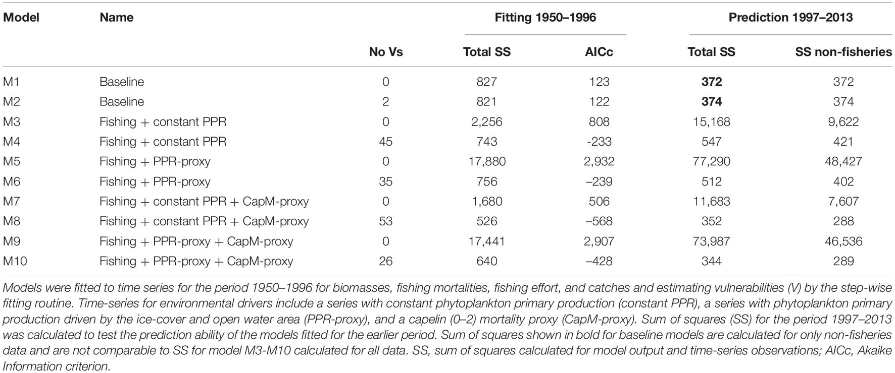
Table 3. Overview of sum of squares for fit (1950–1996) and prediction (1997–2013) for alternative Ecosim models.

For M10, all trophic interactions with estimated vulnerabilities included at least one mammal or fish groups with time-series (Supplementary Table 1). Most (n = 18) of the 26 fitted vulnerabilities were low (vulnerability values < 2) indicating bottom-up effects, and the high vulnerabilities indicating top-down effects were estimated for interactions with top-predators; minke whale, harp seals, Northeast Arctic cod (3+), coastal cod (2+), saithe (3+), and long rough dab (Hippoglossoides platessoides) (Supplementary Table 1). For M8 with 51 estimated vulnerabilities, 29 vulnerabilities were >>2 (Supplementary Table 2) and many estimated vulnerabilities were from trophic interactions with lower trophic level groups without time-series for biomass or catch. Further results presented were based on the M10 model since it had the lowest prediction SS (Table 3).

For the model M10 forced by PPR-proxy and small-herring induced mortality on capelin larvae, modeled biomass time-series for most high trophic level (TL > 3) groups [minke whales, harp seals, Northeast Arctic cod (3+) and saithe (3+)] corresponded well with the observed time-series (Figure 2). For haddock (3+), the modeled biomass was lower than the observed biomass after ca. 2005 (Figure 2). Modeled (M10) and observed time-series for the boreal fisheries-exploited FGs Northeast Arctic cod (3+), minke whale, large redfish, large Greenland halibut and saithe (3+), had relatively high (Spearman r_s > 0.46) positive correlations with modeled values for the period 1950–2013. In contrast, harp seal and pelagic amphipods, had negative correlations (Figure 3). Capelin groups and polar cod (2+) had moderate (r_s from 0.40 to 0.65) positive correlations with modeled values, while polar cod (0–1) and haddock (3+) had no or very low (r_s from 0.0 to 0.06) correlation to modeled values. The ratio of standard deviations showed that the observed time-series of haddock (3+), Scyphozoa, pelagic amphipods and Thysanoessa had high temporal variability and were not highly correlated with the modeled values. Observed time-series of long rough dab and northern shrimp (not shown in Figure 3) also had relatively high temporal variability.

FIGURE 2

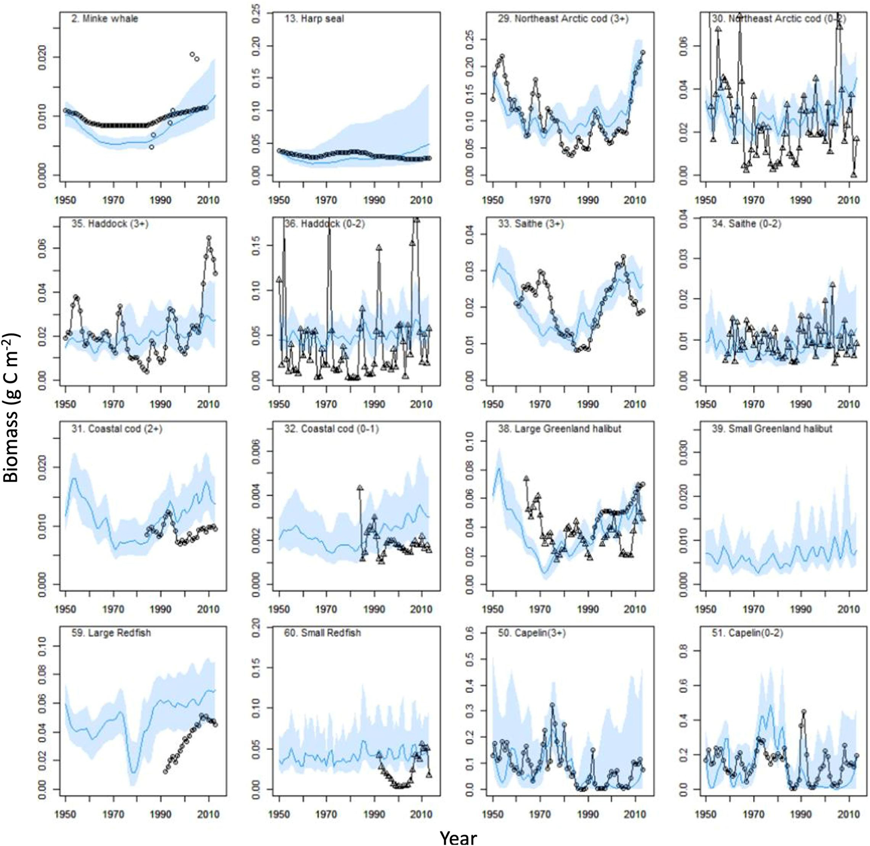
Figure 2. Biomass (g C m^–2) changes for functional groups during 1950–2013 for modeled (model M10, continuous blue line) and observed (circles, absolute biomasses; triangles, relative biomasses). Blue line shows mean value and blue bands shows 2.5 and 97.5 percentiles from 200 Monte Carlo replicates.

FIGURE 3

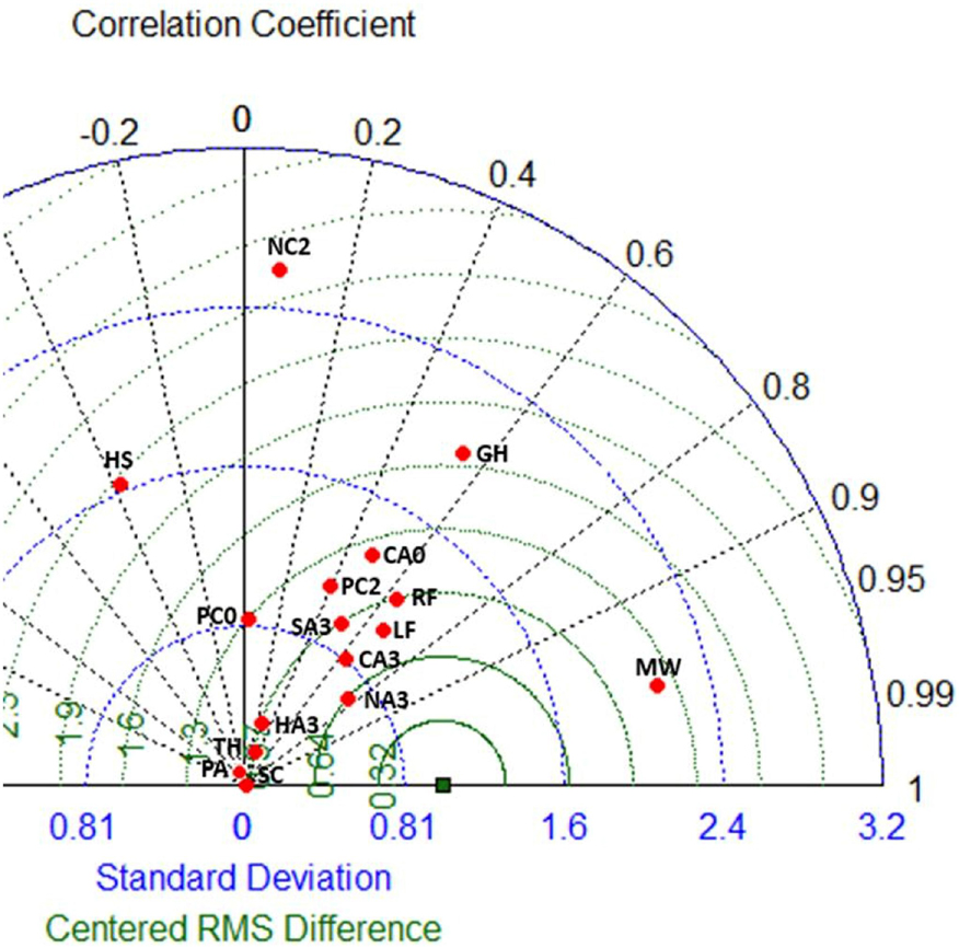
Figure 3. Taylor diagram showing correlation (Pearson r), residual mean square (RMS), and ratio of the standard deviations (scaled) of model simulated (model M10) and observed time-series. Reference point where observed is equal to modeled values is shown by green square. Symbol labels; minke whales (MW), harp seals (HS), Northeast Arctic cod 3+ (NA3), coastal cod 2+ (NC2), saithe 3+ (SA3), haddock 3+ (HA3), large Greenland halibut (GH), large redfish (RFL), capelin 3+ (CA3), capelin 0–2 (CA0), Polar cod 2+ (PC2), polar cod 0–1 (PC0), lumpfish (LF), pelagic amphipods (PA), Thysanoessa (TH), and Scyphomedusae (SC). Groups with higher variability in observed than in modeled time-series, such as haddock age 3+, Thysanoessa, pelagic amphipods, and Scyphomedusae are positioned close to zero scaled deviation ratio.

In the models (M1-M6) lacking mortality forcing on capelin (0–2), the capelin groups in the Ecosim model did not follow the large observed changes from the early 1980s onwards with a large decrease in biomass 1985 and later periodical ups and downs (Figure 2). For the polar cod groups, the modeled biomasses were larger than the observed and the peaks in observed polar cod group biomasses around 2006 was not reproduced by the model which predicted increases in biomass (Supplementary Figure 2).

For northern shrimp, model M10 did not reproduce the peak in observed biomass around 1980, but both model and observed biomass had similar increasing trends after 1990 (Supplementary Figure 2). Biomasses of other pelagic lower trophic level groups, such as Thysanoessa and medium-sized copepods, had more complex temporal variability. Both the modeled Thysanoessa and the observed krill time-series showed an increasing trend during the period 1990–2013, but the simulated biomass time-series did not track the relative large year-to-year changes in the observed krill biomass indices (Supplementary Figure 2). The Russian and Ecosystem survey time-series for krill biomass, were moderately positively correlated for the time period (1980–2005) of overlapping measurements (Spearman r_s = 0.39, P = 0.05).

The modeled biomass for medium-sized copepods and large calanoids had increasing trends after ca. 1995 contrasting the relative stable biomass in the observed mesozooplankton biomass time-series (Supplementary Figure 2). Modeled biomass trends during 1950–2015 for many lower trophic level (TL < 3) groups, i.e., detritivorous polychaetes and large bivalves, showed a similar U-shaped trend as the PPR-proxy with a slight dip in the cold period from 1960 to 1980 (Supplementary Figure 2). The long-lived groups, such as large bivalves and large epibenthic suspension feeders had smoother biomass trajectories and showed a more pronounced U-shape than groups with higher P/B and shorter lifespan, such as detritivorous polychaetes.

The comparison of models with (M11) and without (M10) forcing of ice-algae biomass and production showed that sympagic amphipods were strongly negatively affected by the reduction in ice-coverage after year 2000 (Supplementary Appendix 4 Part G). There were much smaller effects on other groups that fed on ice-algae or ice-algae detritus, but noticeable positive effects of high ice-algae production in the cold 1960–1980 period were found for biomasses of ringed and bearded seals, little auk, and Brünnich’s guillemot. Effects of variable ice-algae production on polar-cod, pelagic amphipods and harp seals were small.

The increase in red king crab and snow crab in the crab-biomass-forced model M12 affected relatively few groups in the comparison to model M13 without crab-biomass forcing (Supplementary Appendix 4 Part E). The magnitude and direction of the effects were closely related to the importance of snow and red king crab in the diet of predators, and the importance of prey groups in the diet of the crab groups. Increasing snow crab and red king crab biomass in model M13 led to a positive effect on predator biomass (e.g., Northeast Arctic cod 3+) and negative effects for crab prey (Supplementary Appendix 4 Part E).

Food Web Structure and Major Flow Pathways

Trophic levels in the BS ecosystem ranged from 1 for primary producers to 5.1 for Polar bear in the year 2000 and 1950 models (Supplementary Appendix 4 Part F). Total biomass, production, consumption and total system throughput were slightly (0.1–11%) lower in the 2000 than in the 1950 model (Table 4). In the year 2000 model, the total ecosystem biomass (13.7 g C m^–2) was mainly comprised of biomass from detritivorous benthic invertebrates (5.3 g C m^–2), phytoplankton (2.0 g C m^–2), other herbivorous zooplankton (1.5 g C m^–2) and krill (1.1 g C m^–2) (Supplementary Table 4). Atlantic cod, the main fishery target, had a biomass of 0.10 g C m^–2.

TABLE 4

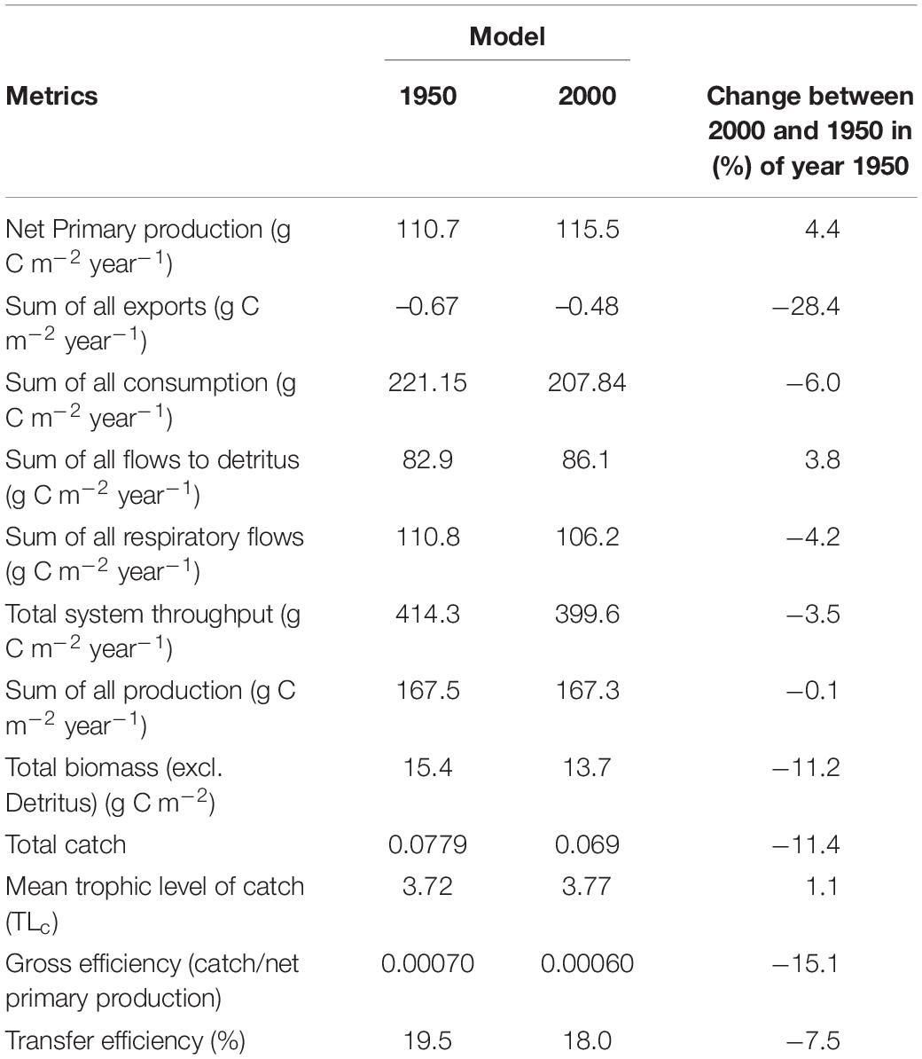
Table 4. Overview of ecosystem metrics for the year 1950 and 2000-Ecopath models.

The total ecosystem production was 167 g C m^–2 yr^–1 with major contributions from the primary producers: phytoplankton (110 g C m^–2 yr^–1) and ice algae (5.3 g C m^–2 yr^–1). At trophic levels between 2 and 3, the main producers were the aggregated compartments microzooplankton and HNAN (19.1 g C m^–2 yr^–1), bacteria (16.1 g C m^–2 yr^–1), other herbivorous zooplankton (8.2 g C m^–2 yr^–1), krill (2.7 g C m^–2 yr^–1) and detritivorous benthic invertebrates (3.1 g C m^–2 yr^–1). At higher trophic levels (TL > 3), major producers were capelin (0.45 g C m^–2 yr^–1), other planktivorous fishes (0.44 g C m^–2 yr^–1) and shrimps (0.17 g C m^–2 yr^–1). Other demersal and benthic fish had a production of 0.17 g C m^–2 yr^–1) and cod had a production of 0.08 g C m^–2 yr^–1. Polar bear, whales, seals, cod, other demersal and benthic fishes, capelin and the zooplankton groups had somewhat higher biomass, production and consumption in the 1950 that the 2000 model (Supplementary Figure 3).

Four major pathways for carbon flow from lower to higher trophic levels were evident for the year 2000 model (Figure 4); the microbial food web pathway, the copepod pathway, the krill pathway and the benthic invertebrate pathway. With regard to the importance as prey, the krill compartment comprised of the FGs Thysanossa and large krill had the most (n = 8) major prey flows (i.e., among the three largest flows to a predator compartment from prey compartments) (Figure 4). Pelagic planktivorous fishes, herbivore zooplankton, and detritus had the second most connections with predator compartments with five major flows. Whereas, krill had major flows to five top-predator compartments, the herbivorous zooplankton compartments had only one major flows to a top-predator compartment (Figure 4).

FIGURE 4

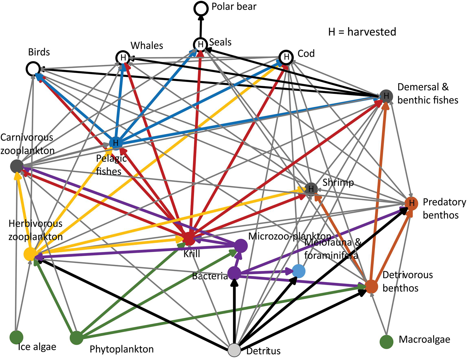
Figure 4. Carbon flows between aggregated major compartments based on the Ecopath model for year 2000 with four major pathways for carbon flows from lower to higher trophic levels. (i) the microbial food-web pathway (violet lines), (ii) the copepod pathway (yellow lines), (iii) the krill pathway (red lines), and (iv) the benthic invertebrate pathway (brown lines). Functional group outputs are aggregated according to Table 1. Thick lines shows major flows, i.e., among the three largest flows to each aggregated compartment. Thin lines shows smaller flows. “H” in circles indicate harvested compartments.

The diet matrix of the year 2000 -model including the snow-crab and red king crab groups had a total of 1,029 feeding interactions and a connectance index of 0.095. The FGs with most groups (n) preying on them were; Thysanoessa (n = 43), pelagic amphipods (n = 35), small herring (n = 33), medium sized copepods (n = 31), capelin age 0–2 (n = 30), and northern shrimp (n = 29).

The five FGs with highest total trophic impact (see Eq. 7) in the year 2000 model were; (1) diatoms, (2) polar cod (2+), (3) Thysanoessa, (4) medium sized copepods and (5) small benthic molluscs (Figure 5). These FGs had contrasting trophic impacts depending on their trophic position (Figure 5). Diatoms had a positive impact as food source for many lower trophic level FGs and had a much larger impact than autotrophic flagellates, the other phytoplankton group (Figure 5). Medium sized copepods and large calanoids had a positive impact as prey for planktivorous fishes and pelagic predatory groups (chaetognaths, cephalopods, Ctenophora, scyphomedusa, and northern shrimp). The krill groups also had a strong positive impact as prey for demersal fishes, some bird groups and several whale and seal FGs (Figure 5). However, the krill groups also had negative impact on some other planktonic invertebrate groups. Capelin and polar cod had positive impacts as prey for demersal fish FGs, seals and some whale groups, and negative impacts as predators on krill, the copepod groups and other pelagic zooplankton FGs (Figure 5). Northeast Arctic cod (3+) had negative impacts as predator on several other fish FGs and positive impact as prey for Greenland shark and dolphins (Figure 5). Northeast Arctic cod also had negative effects on seal and fish FGs that shared prey with cod (Figure 5).

FIGURE 5

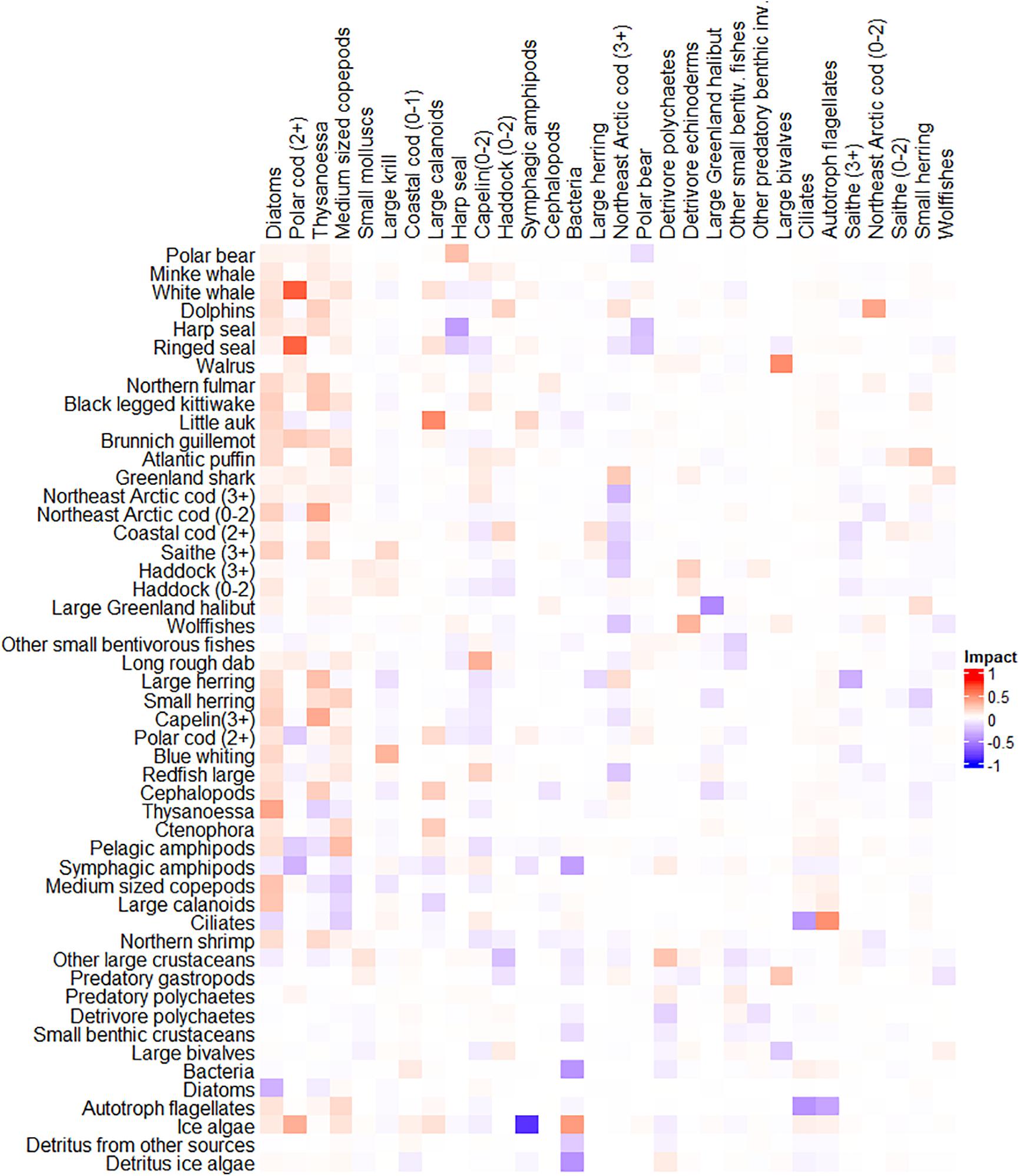
Figure 5. Mixed trophic impact for the year 2000-model. Mixed trophic impacts are shown from the 30 ranked functional groups with highest total impact (column names) on 50 selected impacted functional groups (rows).

Trophic levels estimated by our Ecopath model for year 2000 differed considerably from previously published TL-values from mass-balance models for the BS (Supplementary Table 3). TL-values from our model were on average higher (0.14 and 0.25) than the trophic levels from Dommasnes et al. (2002) and Berdnikov et al. (2019) and lower (–0.21 and –0.25) than the TL’s from Blanchard et al. (2002) and Bentley et al. (2017).

Temporal Variation in Ecosystem Properties and Effects of Exploitation and Climate Variability

The total catch in the BS peaked in the late 1970s mainly driven by the large catches of capelin (Supplementary Figure 5). The catches of mammals decreased during the 1950s and 1960s, stabilized during 1965–1990 and decreased to low levels after 2005 (Supplementary Figure 5). Catches of cod had a decreasing trend from the 1950s and reached a minimum in the period from 1980 to 1990 and then increased to 2013. Other demersal fishes had a peak in the 1970s due to large catches of redfish and Greenland halibut, and had an increase after year 2000 (Supplementary Figures 5, 6).

The trend in the PPR-proxy showed an U-shaped trend with low values in the 1960–1980s (Supplementary Figure 1). Similar U-shaped biomass trends were evident for mammal and birds, total fish biomass, demersal fishes, pelagic invertebrate, and benthic invertebrates group (Supplementary Figure 4). Total biomass of the ecosystem decreased from 1950 to the lowest values around 1970 and thereafter increased toward 2013 (Supplementary Figure 4). In contrast to biomass trends of most other groups, pelagic fish biomass was highest in the period 1970–1980 largely driven by the high capelin biomass at this time.

The Kempton’s diversity index Q changed moderately during 1950–2015 but had lower values at the end of the time-period than in the beginning (Figure 6). Ecosystem P/B for non-primary producing FGs showed a modest increase in the 1970–1980s, but there was a clear peak in P/B for harvested FGs in the 1970–1980s. Trophic level of the catch (TLc) decreased from 1950 to 1985 followed by three periods of ups- and downs corresponding to periods of opening and closure of the capelin fishery (Figure 6).

FIGURE 6

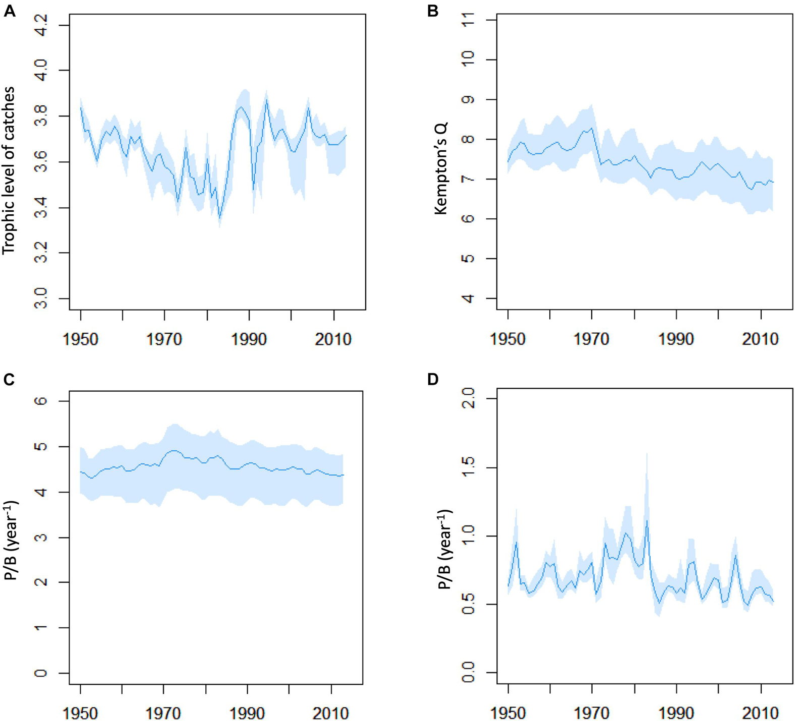
Figure 6. Overview of changes in ecosystem indicators from Ecosim model M10 with Monte Carlo simulations. (A) Trophic level of catch, (B) Kempton’s diversity index Q, (C) total system production/biomass ratio of non-primary producer functional groups, (D) production/biomass ratio based on sum of production and sum of biomass of harvested functional groups. Blue line shows mean value and blue bands shows 2.5 and 97.5 percentiles from 200 Monte Carlo replicates.

Patterns over time for catches and fishing mortalities (F = Y/B) varied substantially between FGs and for Polar bear, minke-whale, harp seals and small herring, catches and catch as proportion of production (Y/P) showed decreasing trends after 1950 (Figure 7 and Supplementary Figures 6, 7). For large Greenland halibut, large redfish, polar cod (2+), northern shrimp and capelin (3+), catches and (Y/P) rose rapidly during the 1970s followed by decreasing trends. Catches of the large gadoids; the Northeast Arctic and coastal cod groups, haddock and saithe, showed temporal variability with low catches in the 1980’s. Y/P for these FGs peaked in the period 1970–1980 and were relatively low after 1980 (Figure 7). Y/P were above 0.5 in periods for all exploited FGs except for Northern shrimp and Polar cod (2+) that had low fishing mortalities and low Y/P’s (Figure 7 and Supplementary Figure 7).

FIGURE 7

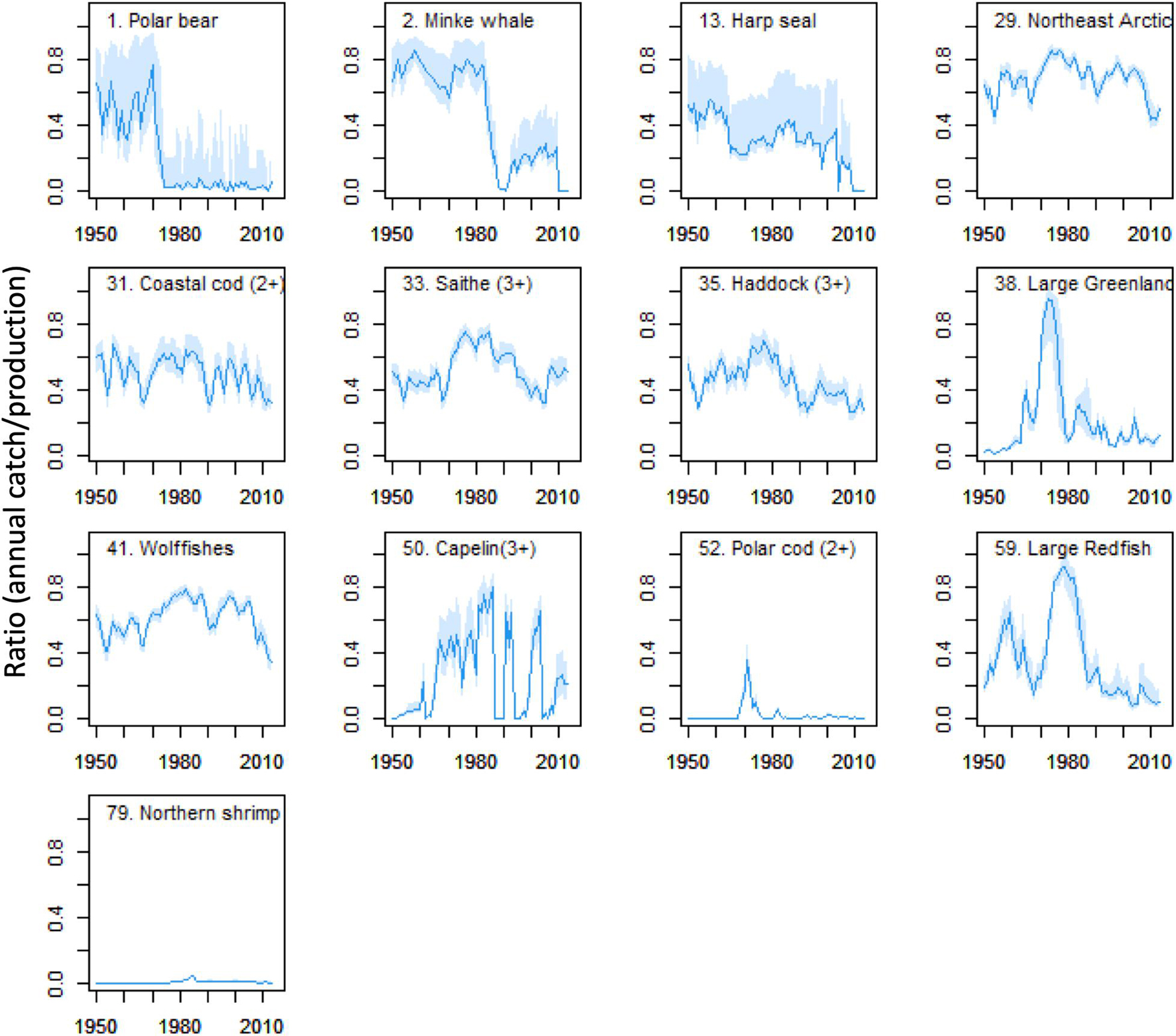
Figure 7. Changes in ratio of catch to production (Y/P) of exploited Ecopath groups during the period 1950–2013. Based on data from M10 Ecosim model. Blue line shows mean value and blue bands shows 2.5 and 97.5 percentiles from Monte Carlo replicates.

Discussion

Main Findings

Intense harvesting had clear negative effects on the biomasses of exploited and long-lived high trophic level FGs, such as mammals, large gadoids, Greenland halibut and redfish. Decrease in fishing pressure the later years contributed to increases of biomasses for many higher trophic level FGs, indicating a recovery period. An increase in primary production after ca. 1990 due to reduced ice-coverage and larger open water area had a positive impact on production and biomass of boreal FGs at all trophic levels.

Model Evaluation and Fitting to Time-Series

The Ecopath models initial values for biomass and production of capelin and polar cod in year 2000 and 1950 did not match the consumption demand from predators and biomasses had to be increased to match the consumption demand. This could be due to underestimation of capelin and polar cod stocks as shown in previous studies (Gjøsæter et al., 1998; Hop and Gjøsæter, 2013). An alternative explanation for the apparent production-consumption mismatch may be that the consumption on planktivorous fish has been overestimated due to bias in the diet composition of predators. Diet data for most predators except for Northeast Arctic cod were not adjusted for possible prey-group-specific differences in digestion rates. Since large fish prey are more slowly digested than smaller prey (Salvanes et al., 1995), predator diet proportions of pelagic fishes may have been overestimated relative to smaller invertebrate prey.

The cross-validation procedure revealed that the model (M8) with fisheries and capelin mortality proxy and constant primary production had a better fit and lower AICc for the fitting period but higher sum of squares for the prediction period than for the model M10 with ice-coverage forced primary production. This led to the conclusion that M10 was the model with most support and this model showed an effect of increasing PPR especially in the last part of the period 1950–2013.

The moderate effects of including snow crab and red king crab FGs in the year 2000 model run with forced biomasses of red king crab and snow crab from year 2000 to 2013 suggest that these FGs were unlikely to have a major effect at the whole ecosystem level during the studied time-period. For red king crab which has a coastal distribution in the southern part of the BS, strong effects on local and regional scale on the bottom fauna have been described (Oug et al., 2011), and similar effects may be expected following ongoing the snow crab expansion.

Comparison With Other Studies

There was a good correspondence between trophic levels estimated for 83 FGs in the Ecopath model for year 2000 and for independent data on trophic levels and δ¹⁵N from stable isotope data from the BS (Pedersen in prep.). The differences between trophic levels estimated by our and other mass-balance models for the BS may be due to between-model differences in group structure and diets of dominant FGs.

Values for biomass, production and consumption of seals, krill, mesozooplankton, and bacteria differ substantially between our model and those published earlier for the BS (Supplementary Table 4). The twice as high food consumption from seals in our model compared to values given by Sakshaug et al. (1994), was mainly due to lower Q/B-values used by Sakshaug et al. (1994). Further, production from krill in our year 2000 Ecopath model was about twice that given by Sakshaug et al. (1994). For both krill groups, we used a higher P/B than Sakshaug et al. (1994) (2.5 vs. 1.5 yr^–1). Production by bacteria in our model was less than 25% of the value given by Sakshaug et al. (1994) and both Sakshaug et al. (1994) and Berdnikov et al. (2019) used much higher P/B-values for bacteria (125–200 year^–1) than in our model (21.2 year^–1). The P/B values for the mesozooplankton, benthic invertebrate and meiofauna FGs in our model were much lower than the values from Blanchard et al. (2002; Supplementary Table 4). Our Ecopath model values for P/B for other herbivore zooplankton including copepods were somewhat higher than estimates derived from other models for Calanus. That our year 2000 model had a lower ecosystem P/B than the 1997 model by Blanchard et al. (2002) (P/B = 12.2 vs. 15.9 year^–1) is likely caused by the lower P/B-values for several low trophic level FGs in our model (Supplementary Table 4). Differences in ecosystem P/B-values are likely to affect how fast the Ecosim models react to perturbations and such effects should be further investigated.

Ecosystem Structure and Major Carbon Flow Pathways and Compartments

The four dominant carbon flows pathways (microbial food web, copepod, krill, and benthic invertebrate pathways) differed regarding P/B of their contributing FGs and their functions as prey sources. The carbon flows within the microbial food web with high P/B and high turnover merges with the krill and copepod pathway and “hitch-hikes” to higher trophic levels. Microzooplankton made up large proportions (10–32%) of the diets of medium zooplankton, large calanoids, small copepods and Thysanoessa in the model, which is consistent with previous studies suggesting a substantial flow from the microbial food web to higher trophic level pelagic FGs in the BS (Hansen et al., 1996; De Laender et al., 2010).

The importance of the copepod pathway was indicated by the high total impact ranks of medium sized copepods and large calanoid copepods, mainly resulting from impacts as prey for planktivorous fish FGs and pelagic carnivorous invertebrate FGs, but also impacts as consumers of microzooplankton and phytoplankton. Copepods are also major prey for early fish stages. In contrast to the krill pathway, the copepod pathway had less direct impact as prey for birds and mammals except as prey for little auks and bowhead whales (Supplementary Appendix 4 Part C).

The krill pathway contributed to an energy-efficient carbon flow to higher trophic levels and top-predators as seen in other ecosystems (Murphy et al., 2007; Ruzicka et al., 2012). The fact that the krill groups were important as prey, but also as a predator and potential competitor for other zooplankton FGs, suggest that krill may have a wasp-waist function in the BS food web. The increase in biomass of krill and corresponding increase in proportion of krill in the diet of age 1–2 year cod after 1984 (Bogstad et al., 2015), suggest increased importance of krill during the last part of the time period. Advection of krill from the Norwegian Sea to the BS was found to be more prominent in warm years (Orlova et al., 2015), and is likely to have contributed to the increased importance of krill in the BS during the warming period.

The detritus-based benthic invertebrate pathway transports carbon to predatory benthos FGs, demersal and benthic fish and also some birds and mammals FGs. Field-based production estimates for macrobenthos for the BS are scarce and uncertain, but local estimates of production range from 0.1 to 20 g C m^–2 year^–1 (Kędra et al., 2013, 2017). Despite the uncertainty, P/B’s (<1.0 year^–1) of the macrobenthos FGs were much lower than for krill and copepods (P/B of c. 2.5–6 year^–1) at similar trophic level. Thus, compared to the pelagic pathways, the benthic invertebrate pathway is a “slow” energy channel with low turnover but high biomass (c. 5 g C m^–2). The presence of pathways or “channels” with different turnover rates and P/B-values may enhance stability in ecosystems (Rooney et al., 2006). Our study emphasize the multi-pathway structure in the BS with a fast partly detritus based microbial food web, a slower pelagic krill pathway in addition to the copepod and benthic invertebrate pathway.

Our model confirms the importance of pelagic planktivorous fish, such as capelin as prey and cod as top-predator emphasized in previous studies (Bogstad et al., 2015). However, in our model, the aggregated compartments “other demersal and benthic fishes” comprising 18 FGs had a total biomass, production and food consumption that was about the twice that of cod in the year 2000 model (Supplementary Table 4). That the consumption of fish by this aggregated compartment was similar to cod indicates a potential for top-down effects from FGs in this compartment and potential for significant competition with cod (Supplementary Table 4).

Effects of Harvesting

Fishing had a major impact on the BS ecosystem during the study period 1950–2013 as indicated by model M10 with predicted biomasses that corresponded well to the observed biomasses of most of the boreal and historically most exploited FGs, including during the latest time period (1996–2013). Optimal exploitation rates (Y/P) depend on life history characteristics, but for fish stocks, optimal Y/P are suggested to be equal to or slightly below 0.5, i.e., fishing and natural mortality being similar (Patterson, 1992; Zhou et al., 2012). The observation that most FGs targeted by the fishery in the BS showed periods when Y/P were larger than 0.5 indicates overexploitation. This is in general accordance with results from single stock assessments (Gjøsæter, 1998; Nakken, 1998; Toresen and Østvedt, 2000). For several fish stocks, especially the long-lived demersal stocks of Greenland halibut, redfish and Northeast Arctic cod, the increases in fishing mortality in the BS from the 1950s to 1970–80s were evident both in the Ecosim-modeled and observed biomass time-series derived from single-stock assessments (Bowering and Nedreaas, 2000; Johannesen et al., 2012). The increase in ecosystem P/B of harvested FGs in the period of highest fishing mortality support that exploitation had a notable effect on ecosystem structure.

Fishing effort and catches increased rapidly after 1945 (Nakken, 1998), and the Norwegian spring-spawning herring was the first fish stock to collapse due to overfishing in the 1960’s (Toresen and Østvedt, 2000). The adult part of this stock is mainly distributed and harvested in the Norwegian Sea, and after the collapse, fishery on juvenile herring which has its major nursery area within the BS was closed in 1971. Following the stock collapse of herring, the capelin fishery expanded in the late 1960s and the 1970s. From the mid-1980s, the BS capelin experienced a series of stock collapses and the variability in total fish catches in the BS and our results show that the trophic level of catches was mainly driven by the state of the capelin fishery. After 1991, the capelin fishery was only open in years when the expected spawning stock was higher than a level estimated by probabilistic assessment accounting for predation from cod on maturing capelin in the pre-spawning period (Gjøsæter et al., 2012). Northeast Arctic cod has been the major fishery target in the BS in terms of fishing effort and commercial value, but is also a major predator on capelin and other smaller fish and invertebrates (Bogstad et al., 2015). After a period of increasing fishing mortality after 1950, the decrease in fishing mortality of this large stock after ca. 1990 contributed strongly to the recovery and increase in stock biomass, production and catches (Nakken et al., 1996).

The populations of the large baleen whales (bowhead, blue, and fin whales) and walruses were heavily exploited and reduced to levels far below pristine levels prior to 1950 (Reeves, 1980; Christensen et al., 1992; Weslawski et al., 2000) and Greenland shark was also exploited before and to a low extent after 1950 (Supplementary Appendix 2). For minke whales and harp seals, catches and harvesting mortalities were reduced to lower levels during the period 1950–2013. Biomass trends for these exploited mammal FGs were U-shaped and showed trends of recovery as a result of reduced exploitation and increased ecosystem productivity.

The sequence in which fisheries evolved in the BS resembles a pattern consistent with the “Fishing through the food web” concept (Branch et al., 2010). However, the sequence in which the fisheries targeted various FGs may have been directed by availability rather than trophic level. Fishing pressure on pelagic intermediate trophic level fishes, such as herring and capelin were increasing relatively early in the study period, simultaneously with pressure on Northeast Arctic cod. This may have contributed to a kind of trophic balance when both typical prey and predator FGs were exploited simultaneously. Nilsen et al. (2020) explored balanced harvesting strategies for the Norwegian and BS using the Atlantis model and found that a balanced harvesting regime would only produce marginal increases in total yield of currently exploited FGs compared to the historical exploitation regime after 1980.

Most harvested fish stocks responded with an increase in biomass when fishing mortality (Y/B) decreased in the 1990’s (Nakken, 1998) indicating a recovery period. The patterns of catches, biomasses and fishing mortality indicate that the intense exploitation was relaxed around 1990–2000 for many of the targeted fish and exploited mammal FGs and contributed to increases in their biomasses. The Golden Redfish (S. norvegicus) stock and the Coastal cod stock have not fully recovered (ICES, 2019), and may be exceptions to the recovery pattern described above.

Recent studies have shown that the dynamics of cod is tightly linked to the harvesting rate and capelin abundance (Lindstrøm et al., 2009; Koen-Alonso et al., 2021). If their top-down control was dominating in the BS ecosystem, prey groups would expected to be “released” from predation and increase during periods of heavy exploitation i.e., from ca. 1970 to 1990 when some predator stocks, e.g., Northeast Arctic cod and Greenland halibut, were reduced to low levels. One would also expect that the biomass of competitors would increase simply due to reduced competition. The question is if there is any evidence of trophic-cascade and competitive-release effects in the model? The predicted increase in biomass of capelin and long rough dab during this period by the M10 Ecosim model suggest cascade effects due to reduced predation pressure. The period of high biomass of capelin in the period 1970–1985 was likely a result of reduced predation from small herring predation on capelin larvae during the period of collapse of the Norwegian spring spawning herring. In addition, low levels of predation from demersal fishes and cod on older capelin may have contributed to the high capelin biomass level. The increase in modeled biomass of long rough dab during 1970–1990 cannot be verified by survey observations since the stock-assessment time-series started in 1989 (Supplementary Appendix 4 Part A,B).

Among the other FGs, northern shrimp had the longest observational time-series, starting in 1971, and the very low fishing mortality compared to the predation mortality suggests that fishery exploitation had not been a dominant driver for this stock. Decreases in cod stocks in the Northwestern Atlantic have been accompanied by sharp increases in biomass of invertebrate stocks, and this has been interpreted as results of a trophic cascade (Frank et al., 2005). In the BS, however, several shrimp-predating FGs may have increased when the cod stock decreased contributing to a relative stable predation pressure and modest biomass changes for northern shrimp. Thus, we suggest that except for capelin, there is little evidence for a strong cascading effect of medium and low trophic level FGs during the period of low top predator abundance in the BS.

The Ecosim-simulated biomass of detritivorous and predatory macrobenthos showed a U-shape during 1960–1990 that could be attributed to the relative low water temperature, small open-water area (=extensive ice-cover) and low primary production. There was no available time-series of macrobenthos biomass at the ecosystem level, but estimates based on grab sampling over a large part of the BS have changed over time from high biomass in 1924–32, to low biomass in 1968–72 and then high biomass in 2003 again (Denisenko, 2001; Jørgensen et al., 2017). The changes in biomass among time-periods have been attributed to changes in both climate and primary production and to changes in bottom trawling effort hypothesized to affect macrobenthic biomass negatively (Denisenko, 2001). To simulate and evaluate the possible direct effects of bottom trawling in Ecosim, a relationship between bottom trawling effort and mortality for various FGs of benthic invertebrates have to be included in future simulations.

The moderate changes in the Kempton diversity index, which is expected to react to intense exploitation during the period 1950–2013, suggest modest changes in ecosystem structure. So why and how has the ecosystem resisted the heavy exploitation of some FGs? The high fishing effort during the period 1965–1990 in the cod fishery in the BS have likely also increased fishing mortality of other fish FGs which were caught as bycatch (Denisenko, 2001; Rusyaev and Orlov, 2013). In the BS, there may have been few species that could take over for cod as major piscivore during the period of intense exploitation, and candidates, such as Greenland halibut, redfish and harp seals had been extensively targeted and reduced by harvesting prior and during the cold period.

Effects of Climate Variability

The U-shaped trend in biomass of many FGs is interpreted as mainly a result of trends in primary production. Models forced by the PPR-proxy performed better during the warm period (after mid 1990s) suggesting that more open water is linked to increased PPR and food web productivity. Earlier studies have emphasized the positive effects of relatively warm Atlantic water in the southern part of the BS on fish stock recruitment and individual fish growth (Sundby, 2000; Ottersen et al., 2002), especially for Northeast Arctic cod, haddock and Norwegian spring spawning herring partly spawning in the Norwegian Sea (Bogstad et al., 2013). High variability in haddock recruitment lead to relatively low predictability by Ecosim for haddock (3+) biomass. The relatively low temporal model fit to the indices (relative biomasses) for the youngest stanza of the cod and haddock groups suggest that recruitment may be driven partly by other mechanisms than represented by the PPR-proxy, and further testing of other drivers for recruitment may improve model fits and predictability. Variability in advection of Atlantic water and copepods, krill and young fish stages into the southwestern part of the BS affect the ecosystem (Drinkwater, 2011), and is likely to contribute to variability that was not captured by the Ecosim models.

The correlations between modeled and observed data for the unharvested lower trophic-level FGs were lower than for the most heavily exploited FGs and may be due to a lower signal to noise ratio for observed data for these FGs. The lower trophic level FGs also had higher temporal variability than for the more long-lived higher trophic level FGs. This indicates that the Ecosim model did not fully reproduce short-term variability in lower trophic level FGs but could still capture the main long-term trends.

The proxy for PPR that was applied in the calibration and fitting to time-series in Ecosim was based on a well-founded relationship between primary production and open-water area (Dalpadado et al., 2020). This relationship is supported by model studies showing lower primary production at lower temperature, and temperature and open water area were strongly positively correlated (Wassmann et al., 2006b; Slagstad et al., 2011). The improvement in model prediction by including our PPR-proxy as an environmental driver in the model suggests that changes in PPR driven by changes in open-water area and indirectly by water temperature had an effect on the development of the BS ecosystem during the 1950–2013 period.

The lower trophic level FGs for which we had observed biomass time-series (krill and mezozooplankton, pelagic amphipods, and scyphomedusae) showed contrasting trends after year 1995. The observed biomasses of the two krill groups and scyphomedusae showed increasing trends from year 2000 to 2013 while there was a stable biomass of mesozooplankton (Dalpadado et al., 2020) and a decreasing trend for pelagic amphipod biomass. The Ecosim model, however, predicted an increase in biomass of medium sized copepod and large calanoid biomasses after 1995. Mesozooplankton biomass is dominated by the mainly boreal medium sized copepods and the arctic large calanoids, and these FGs may have responded differently to warming in the western part of the BS after 1995 (Aarflot et al., 2017). Biophysical modeling with warming scenarios show expectations of increased production the boreal C. finmarchicus and decreased production in the arctic C. glacialis (Slagstad et al., 2011). Predation from capelin has been emphasized to have a major top-down effect on mesozooplankton in the BS, but after a peak in observed biomass mesozooplankton around 1994 when capelin biomass was low, mesozooplankton biomass has been stable despite ups and downs in capelin biomass (Dalpadado et al., 2020). Stige et al. (2019) suggested that less sea-ice coverage may have a negative effect on the arctic large calanoid C. glacialis.

The krill biomass in the BS was dominated by Thysanoessa, and krill had the longest observed time-series among lower trophic level FGs. Increases in both observed and modeled krill biomass in the period after ca. 1995 indicates that the energy-efficient krill pathway may have strengthened during the period 2000–2013. Krill as prey may have contributed to shorten the food chains and enhance production at high trophic levels. The temporal year-to-year variability in the observed krill time-series was not well-reproduced by the model. That the observational time-series for the two krill groups were moderately positively correlated may indicate that they both represent temporal trend in the krill biomass but with a relatively low signal to noise ratio. It is challenging to estimate biomass of krill precisely due to very patchy spatial distribution (Eriksen et al., 2016) and varying advection of krill into the BS may also contribute to variability (Orlova et al., 2015).

The modeled effects of a decreasing trend in sea-ice coverage and reduced ice-algae production (model M11) after ca. 1980 notably affected biomasses of ringed and bearded seals, little auks, and Brünnich’s guillemots. Polar cod and pelagic amphipods were less affected and variable ice-algae production could not explain the observed decreasing time-trends in these predator FGs after ca. year 2000. This may indicate that sea-ice may be a limiting habitat for these FGs beyond the production of ice-algae. Sea-ice coverage is important for polar cod during reproduction and recruitment and both large calanoid copepods and pelagic amphipods feed on ice algae and these FGs are important prey for polar cod (Hop and Gjøsæter, 2013; Bouchard and Fortier, 2020; Supplementary Appendix 2). More knowledge on the dependence of the ice-habitat habitat beyond the effect of ice-algae production and other effects of warming, may be needed to improve model input and performance.

The Ecopath model output suggests that scyphomedusae did not have a major predatory effect in the BS ecosystem despite its increase in the warm period after year 2000 (Eriksen, 2016). For Ctenophora, there was no time-series or precise biomass estimate, but recordings of frequency of occurrence of Ctenophora in Northeast Arctic cod stomachs shows a clear increase after 1996 in the southwestern BS (Eriksen et al., 2018), and may suggest an increase in biomass of Ctenophora in the area during this period.

The inclusion of mortality from small herring on capelin larvae in the Ecosim model increased the model fit to observed data by primarily improving the fit for the capelin groups but not for the other FGs. This may suggest that top-down and bottom-up effects of capelin in the Ecosim model were moderate during the modeled time-period. An apparent top-down effect from capelin as predator on krill has been observed (Eriksen and Dalpadado, 2011), and field measurements revealed that biomasses of capelin and total mesozooplankton varied inversely during 1989–1997 but not in the period after 1997 (Dalpadado et al., 2020). Strong negative effects of low capelin biomass on predators, such as Northeast Arctic cod and harp seals were observed during the first capelin collapse in 1985–1988 (Gjøsæter et al., 2009), but effects were lower during later collapses, likely due to larger abundance of alternative prey (Gjøsæter et al., 2009). This inconsistency in correlations suggests complex trophic interactions and potential indirect effects that are difficult to identify from modeled or observed time-series.

The patterns of mixed trophic impacts for various Ecopath model FGs showed that most FGs had both bottom-up and top-down impacts, suggesting that both types of trophic control have been important in the BS and other studies also point in this direction (Johannesen et al., 2012; Lindstrøm et al., 2017; Stige et al., 2019). By examining predator-prey correlations from the BS, Johannesen et al. (2012) found shifts between negative and positive correlations during the time period 1977–2002, indicating shifts in trophic control between bottom-up and top-down dominance. Stige et al. (2019) also noted that both bottom-up and top-down effects were present when considering pelagic fish and zooplankton interactions.

Lower fishing mortalities coinciding with warming and increasing primary production during the recovery period after around 1990 may have strengthened the role of cod and other demersal fishes as top predators. The coincidence of the period of overexploitation of fish stocks with the cold low-productive climatic period during 1960–1980 may have prevented other species to take over when the stocks of large gadoids and the long-lived redfish and Greenland halibut had been intensively exploited and reduced. The relatively low diversity of the non-exploited fish FGs in the BS may also have contributed to the lack of success of other species to replace exploited stocks. How ecosystem management can be used to preserve structure and mitigate negative climatic effects should be investigated in future studies.

Conclusion

Four major carbon pathways were identified in the BS and the modeling results indicated increased productivity at lower trophic levels during warm years with large ice-free open-water area after ca. 2000. This contributed to higher productivity for most high trophic level FGs. The krill pathway was important for both medium and high trophic level compartments, and krill biomass and production increased during the warm period. There were signs of decrease in observed biomasses of some high arctic FGs that were not reproduced by the models even after forcing the model ice-algae with ice coverage time-series.

In the low-productive period from 1960 to 1985, fishery exploitation reduced biomasses of FGs in a sequential pattern causing reductions of biomasses for mammals, large gadoids and other long-lived demersal fishes. The increased biomass for capelin during this period was interpreted as a trophic cascade effect of relaxed predation. When exploitation was relaxed, biomasses of many exploited FGs increased during the recovery period after about 1990. Despite heavy exploitation, the basic ecosystem structure seems to have been preserved in the BS during the periods of overexploitation and recovery.

Data Availability Statement

The original contributions presented in the study are included in the article/Supplementary Material, further inquiries can be directed to the corresponding author/s.

Ethics Statement

Ethical review and approval was not required for the animal study because this was a modeling study using historical data and as such we did not need ethical review and approval.

Author Contributions

TP developed the initial model concept and structure and implemented the models. NM contributed to the data structuring. TP, NM, UL, and PR contributed to the ideas in this manuscript and drafted the manuscript. All authors contributed to the data input, provided edits to the manuscript, contributed to the article, and approved the submitted version.

Funding

This Norway-Canada collaborative project “A Transatlantic innovation area for sustainable development in the Arctic” (CoArc) provided partial support for this work (Project Number 8048 at Akvaplan-Niva and QZ-15/0457 at Norwegian Ministry of Foreign Affairs). The Research Council of Norway also provided partial support through the project “The Nansen Legacy” (RCN#276730).

Conflict of Interest

PR and HB were employed by company Akvaplan-Niva AS. IE was employed by SINTEF Ocean.

The remaining authors declare that the research was conducted in the absence of any commercial or financial relationships that could be construed as a potential conflict of interest.

Publisher’s Note

All claims expressed in this article are solely those of the authors and do not necessarily represent those of their affiliated organizations, or those of the publisher, the editors and the reviewers. Any product that may be evaluated in this article, or claim that may be made by its manufacturer, is not guaranteed or endorsed by the publisher.

Acknowledgments

We would like to thank Bjarte Bogstad and Martin Biuw at Institute of Marine Research, Norway for providing cod stomach summary data and harp seal data, respectively. We thank Leif C. Stige at University of Oslo for providing time-series on pelagic amphipods.

Supplementary Material

The Supplementary Material for this article can be found online at: https://www.frontiersin.org/articles/10.3389/fmars.2021.732637/full#supplementary-material

Footnotes

1. ^ http://www.pinro.ru/labs/hid/kolsec22.php?lang
2. ^ http://ecopath.org

References

Aarflot, J. M., Skjoldal, H. R., Dalpadado, P., and Skern-Mauritzen, M. (2017). Contribution of Calanus species to the mesozooplankton biomass in the Barents Sea. ICES J. Mar. Sci. 75, 2342–2354. doi: 10.1093/icesjms/fsx221

CrossRef Full Text | Google Scholar

Ainsworth, C. H., and Pitcher, T. J. (2006). Modifying Kempton’s species diversity index for use with ecosystem simulation models. Ecol. Indic. 6, 623–630. doi: 10.1016/j.ecolind.2005.08.024

CrossRef Full Text | Google Scholar

Akaike, H. (1974). A new look at the statistical model identification. IEEE Trans. Autom. Control 19, 716–723. doi: 10.1109/tac.1974.1100705

CrossRef Full Text | Google Scholar

Andriyashev, A., and Chernova, N. (1995). Annotated list of fishlike vertebrates and fish of the arctic seas and adjacent waters. J. Ichthyol. 35, 81–123.

Google Scholar

Araujo, J., and Bundy, A. (2012). Effects of environmental change, fisheries and trophodynamics on the ecosystem of the western Scotian Shelf, Canada. Mar. Ecol. Prog. Series 464, 51–67. doi: 10.3354/meps09792

CrossRef Full Text | Google Scholar

Bentley, J. W., Serpetti, N., and Heymans, J. J. (2017). Investigating the potential impacts of ocean warming on the Norwegian and Barents Seas ecosystem using a time-dynamic food-web model. Ecol. Mod. 360, 94–107. doi: 10.1016/j.ecolmodel.2017.07.002

CrossRef Full Text | Google Scholar

Berdnikov, S., Kulygin, V., Sorokina, V., Dashkevich, L., and Sheverdyaev, I. (2019). An integrated mathematical model of the large marine ecosystem of the Barents Sea and the White Sea as a tool for assessing natural risks and efficient use of biological resources. Doklady Earth Sci. 487, 963–968. doi: 10.1134/s1028334x19080117

CrossRef Full Text | Google Scholar

Bergmeir, C., and Benítez, J. M. (2012). On the use of cross-validation for time series predictor evaluation. Inform. Sci. 191, 192–213. doi: 10.1016/j.ins.2011.12.028

CrossRef Full Text | Google Scholar

Blanchard, J., Pinnegar, J., and Mackinson, S. (2002). Exploring marine mammal-fishery interactions using ‘Ecopath with Ecosim’: modelling the Barents Sea ecosystem. Sci. Ser. Tech Rep. CEFAS Lowestoft 117:52.

Google Scholar

Bogstad, B., Dingsør, G. E., Ingvaldsen, R. B., and Gjøsæter, H. (2013). Changes in the relationship between sea temperature and recruitment of cod, haddock and herring in the Barents Sea. Mar. Biol. Res. 9, 895–907. doi: 10.1080/17451000.2013.775451

CrossRef Full Text | Google Scholar

Bogstad, B., Gjøsæter, H., Haug, T., and Lindstrøm, U. (2015). A review of the battle for food in the barents sea: cod vs. marine mammals. Front. Ecol. Evolu. 3:1–17.

Google Scholar

Bouchard, C., and Fortier, L. (2020). The importance of Calanus glacialis for the feeding success of young polar cod: a circumpolar synthesis. Polar Biol. 43, 1095–1107. doi: 10.1007/s00300-020-02643-0

PubMed Abstract | CrossRef Full Text | Google Scholar

Bowering, W. R., and Nedreaas, K. H. (2000). A comparison of Greenland halibut (Reinhardtius hippoglossoides (Walbaum)) fisheries and distribution in the Northwest and Northeast Atlantic. Sarsia 85, 61–76. doi: 10.1080/00364827.2000.10414555

CrossRef Full Text | Google Scholar

Branch, T. A., Watson, R., Fulton, E. A., Jennings, S., McGilliard, C. R., Pablico, G. T., et al. (2010). The trophic fingerprint of marine fisheries. Nature 468, 431–435. doi: 10.1038/nature09528

PubMed Abstract | CrossRef Full Text | Google Scholar

Christensen, I., Haug, T., and Øien, N. (1992). Seasonal distribution, exploitation and present abundance of stocks of large baleen whales (Mysticeti) and sperm whales (Physeter macrocephalus) in Norwegian and adjacent waters. ICES J. Mar. Sci. 49, 341–355. doi: 10.1093/icesjms/49.3.341

CrossRef Full Text | Google Scholar

Christensen, V., and Pauly, D. (1992). ECOPATH IIa software for balancing steady-state ecosystem models and calculating network characteristics. Ecol. Mod. 61, 169–185. doi: 10.1016/0304-3800(92)90016-8

CrossRef Full Text | Google Scholar

Christensen, V., Walters, C., and Pauly, D. (2005). Ecopath with Ecosim: A User’s Guide. Vancouver: Fisheries Centre of University of British Columbia.

Google Scholar

Christensen, V., and Walters, C. J. (2004). Ecopath with Ecosim: methods, capabilities and limitations. Ecol. Mod. 172, 109–139. doi: 10.1016/j.ecolmodel.2003.09.003

CrossRef Full Text | Google Scholar

Coll, M., Bundy, A., and Shannon, L. J. (2009). “Ecosystem modelling using the ecopath with ecosim approach,” in Computers in Fisheries Research, eds B. A. Megrey and E. Moksness (Springer), 225–291. doi: 10.1007/978-1-4020-8636-6_8

CrossRef Full Text | Google Scholar

Dalpadado, P., Arrigo, K. R., Hjøllo, S. S., Rey, F., Ingvaldsen, R. B., Sperfeld, E., et al. (2014). Productivity in the barents sea-response to recent climate variability. PLoS One 9:e95273. doi: 10.1371/journal.pone.0095273

PubMed Abstract | CrossRef Full Text | Google Scholar

Dalpadado, P., Arrigo, K. R., van Dijken, G. L., Skjoldal, H. R., Bagøien, E., Dolgov, A., et al. (2020). Climate effects on temporal and spatial dynamics of phytoplankton and zooplankton in the Barents Sea. Progr. Oceanogr. 185:102320. doi: 10.1016/j.pocean.2020.102320

CrossRef Full Text | Google Scholar

De Laender, F., Oevelen, D. V., Soetaert, K., and Middelburg, J. J. (2010). Carbon transfer in herbivore-and microbial loop-dominated pelagic food webs in the southern barents sea during spring and summer. Mar. Ecol. Prog. Series 398, 93–107. doi: 10.3354/meps08335

CrossRef Full Text | Google Scholar

Denisenko, S. (2001). Long-term changes of zoobenthos biomass in the barents sea. Proc. Zool. Inst. Russ. Acad. Sci. 289, 59–66.

Google Scholar

Dippner, J. W., and Ottersen, G. (2001). Cod and climate variability in the barents sea. Climate Res. 17, 73–82. doi: 10.3354/cr017073

CrossRef Full Text | Google Scholar

Dommasnes, A., Christensen, V., Ellertsen, B., Kvamme, C., Melle, W., Nøttestad, L., et al. (2002). “An ECOPATH model for the norwegian and barents sea. fisheries impact on north atlantic ecosystems: models and analyses. fisheries centre research reports no. 9(4),” in Fisheries Centre Research Reports, eds S. Guénette, V. Christensen, and D. Pauly (Vancouver).

Google Scholar

Drinkwater, K. F. (2011). The influence of climate variability and change on the ecosystems of the barents sea and adjacent waters: review and synthesis of recent studies from the NESSAS Project. Progr. Oceanogr. 90, 47–61. doi: 10.1016/j.pocean.2011.02.006

CrossRef Full Text | Google Scholar

Eriksen, E. (2016). Do scyphozoan jellyfish limit the habitat of pelagic species in the barents sea during the late feeding period? ICES J. Mari. Sci. 73, 217–226. doi: 10.1093/icesjms/fsv183

CrossRef Full Text | Google Scholar

Eriksen, E., Bogstad, B., Dolgov, A., and Beck, I. (2018). Cod diet as an indicator of Ctenophora abundance dynamics in the barents sea. Mari. Ecol. Prog. Series 591, 87–100. doi: 10.3354/meps12199

CrossRef Full Text | Google Scholar

Eriksen, E., Bogstad, B., and Nakken, O. (2011). Ecological significance of 0-group fish in the barents sea ecosystem. Polar Biol. 34, 647–657. doi: 10.1007/s00300-010-0920-y

CrossRef Full Text | Google Scholar

Eriksen, E., and Dalpadado, P. (2011). Long-term changes in Krill biomass and distribution in the Barents Sea: are the changes mainly related to capelin stock size and temperature conditions? Polar Biol. 34, 1399–1409. doi: 10.1007/s00300-011-0995-0

CrossRef Full Text | Google Scholar

Eriksen, E., Skjoldal, H. R., Dolgov, A. V., Dalpadado, P., Orlova, E. L., and Prozorkevich, D. V. (2016). The Barents Sea euphausiids: methodological aspects of monitoring and estimation of abundance and biomass. ICES J. Mari. Sci. 73, 1533–1544. doi: 10.1093/icesjms/fsw022

CrossRef Full Text | Google Scholar

Eriksen, E., Skjoldal, H. R., Gjøsæter, H., and Primicerio, R. (2017). Spatial and temporal changes in the Barents Sea pelagic compartment during the recent warming. Progr. Oceanogr. 151, 206–226. doi: 10.1016/j.pocean.2016.12.009

CrossRef Full Text | Google Scholar

Fauchald, P., Anker-Nilssen, T., Barrett, R., Bustnes, J. O., Bårdsen, B.-J., Christensen-Dalsgaard, S., et al. (2015). The Status and Trends of Seabirds Breeding in Norway and Svalbard. NINA Report 1151.

Google Scholar

Fogarty, M., Incze, L., Hayhoe, K., Mountain, D., and Manning, J. (2008). Potential climate change impacts on Atlantic cod (Gadus morhua) off the northeastern USA. Mitigat. Adapt. Strat. Glob. Change 13, 453–466.

Google Scholar

Fossheim, M., Primicerio, R., Johannesen, E., Ingvaldsen, R. B., Aschan, M. M., and Dolgov, A. V. (2015). Recent warming leads to a rapid borealization of fish communities in the Arctic. Nat. Climate Change 5:673. doi: 10.1038/nclimate2647

CrossRef Full Text | Google Scholar

Frank, K. T., Petrie, B., Choi, J. S., and Leggett, W. C. (2005). Trophic cascades in a formerly cod-dominated ecosystem. Science 308, 1621–1623. doi: 10.1126/science.1113075

PubMed Abstract | CrossRef Full Text | Google Scholar

Fulton, E. A., Smith, A. D. M., and Punt, A. E. (2005). Which ecological indicators can robustly detect effects of fishing? ICES J. Mari. Sci. 62, 540–551. doi: 10.1016/j.icesjms.2004.12.012

CrossRef Full Text | Google Scholar

Gaichas, S., Skaret, G., Falk-Petersen, J., Link, J. S., Overholtz, W., Megrey, B. A., et al. (2009). A comparison of community and trophic structure in five marine ecosystems based on energy budgets and system metrics. Progr. Oceanogr. 81, 47–62. doi: 10.1016/j.pocean.2009.04.005

CrossRef Full Text | Google Scholar

Gjøsæter, H. (1998). The population biology and exploitation of capelin (Mallotus villosus) in the Barents sea. Sarsia 83, 453–496. doi: 10.1080/00364827.1998.10420445

CrossRef Full Text | Google Scholar

Gjøsæter, H., Bogstad, B., and Tjelmeland, S. (2009). Ecosystem effects of the three capelin stock collapses in the Barents Sea. Mari. Biol. Res. 5, 40–53. doi: 10.1080/17451000802454866

CrossRef Full Text | Google Scholar

Gjøsæter, H., Dommasnes, A., and Røttingen, B. (1998). The Barents Sea capelin stock 1972–1997. a synthesis of results from acoustic surveys. Sarsia 83, 497–510. doi: 10.1080/00364827.1998.10420446

CrossRef Full Text | Google Scholar

Gjøsæter, H., Hallfredsson, E. H., Mikkelsen, N., Bogstad, B., and Pedersen, T. (2015). Predation on early life stages is decisive for year-class strength in the Barents Sea capelin (Mallotus villosus) stock. ICES Journal of Marine Science. J. du Conseil 73, 165–181. doi: 10.1093/icesjms/fsv177

CrossRef Full Text | Google Scholar

Gjøsæter, H., Tjelmeland, S., and Bogstad, B. (2012). “Ecosystem-based management of fish species in the Barents Sea,” in Global Progress in Ecosystem Based Fisheries Management, eds G. H. Kruse, H. I. Browman, K. L. Cochrane, D. Evans, G. S. Jamieson, P. A. Livingston, et al. (Alaska Sea Grant, University of Alaska Fairbanks), 333–352. doi: 10.4027/gpebfm.2012.017

CrossRef Full Text | Google Scholar

Halpern, B. S., Walbridge, S., Selkoe, K. A., Kappel, C. V., Micheli, F., D’Agrosa, C., et al. (2008). A global map of human impact on marine ecosystems. Science 319, 948–952.

Google Scholar

Hansen, B., Christiansen, S., and Pedersen, G. (1996). Plankton dynamics in the marginal ice zone of the central Barents Sea during spring: carbon flow and structure of the grazer food chain. Polar Biol. 16, 115–128. doi: 10.1007/s003000050036

CrossRef Full Text | Google Scholar

Hansen, C., Skern-Mauritzen, M., van der Meeren, G., Jähkel, A., and Drinkwater, K. (2016). Set-up of the Nordic and Barents Seas (NoBa) Atlantis model. Fisken og Havet No 2/2016. Institute of Marine Research, Bergen.

Google Scholar

Haug, T., Bogstad, B., Chierici, M., Gjøsæter, H., Hallfredsson, E. H., Høines, ÅS., et al. (2017). Future harvest of living resources in the arctic ocean north of the nordic and barents seas: a review of possibilities and constraints. Fish. Res. 188, 38–57. doi: 10.1016/j.fishres.2016.12.002

CrossRef Full Text | Google Scholar

Heymans, J. J., Coll, M., Libralato, S., Morissette, L., and Christensen, V. (2014). Global patterns in ecological indicators of marine food webs: a modelling approach. PLoS One 9:e95845. doi: 10.1371/journal.pone.0095845

PubMed Abstract | CrossRef Full Text | Google Scholar

Heymans, J. J., Coll, M., Link, J. S., Mackinson, S., Steenbeek, J., Walters, C., et al. (2016). Best practice in Ecopath with Ecosim food-web models for ecosystem-based management. Ecol. Mod. 331, 173–184. doi: 10.1016/j.ecolmodel.2015.12.007

CrossRef Full Text | Google Scholar

Hop, H., and Gjøsæter, H. (2013). Polar cod (Boreogadus saida) and capelin (Mallotus villosus) as key species in marine food webs of the Arctic and the Barents Sea. Mari. Biol. Res. 9, 878–894. doi: 10.1080/17451000.2013.775458

CrossRef Full Text | Google Scholar

Hsieh, C.-h., Reiss, C. S., Hewitt, R. P., and Sugihara, G. (2008). Spatial analysis shows that fishing enhances the climatic sensitivity of marine fishes. Canad. J. Fish. Aquat. Sci. 65, 947-961.

Google Scholar

Hunt, G. L., Blanchard, A. L., Boveng, P., Dalpadado, P., Drinkwater, K. F., Eisner, L., et al. (2013). The barents and chukchi seas: comparison of two arctic shelf ecosystems. J. Mari. Syst. 109, 43–68.

Google Scholar

ICES. (2019). Arctic fisheries working group (AFWG). ICES Sci. Rep. 1:30. doi: 10.17895/ices.pub.15292

CrossRef Full Text | Google Scholar

Jackson, J. B. (2001). Historical overfishing and the recent collapse of coastal ecostsystems. Science 293, 629–638. doi: 10.1126/science.1059199

PubMed Abstract | CrossRef Full Text | Google Scholar

Johannesen, E., Ingvaldsen, R. B., Bogstad, B., Dalpadado, P., Eriksen, E., Gjøsæter, H., et al. (2012). Changes in Barents Sea ecosystem state, 1970–2009: climate fluctuations, human impact, and trophic interactions. ICES J. Mari. Sci. 69, 880–889. doi: 10.1093/icesjms/fss046

CrossRef Full Text | Google Scholar

Jørgensen, L. L., Archambault, P., Blicher, M., Denisenko, N., Guðmundsson, G., Iken, K., et al. (2017). State of the Arctic Marine Biodiversity Report. Conservation of Arctic Flora and Fauna (CAFF). Akureyri: Benthos, 85–107.

Google Scholar

Jørgensen, L. L., Ljubin, P., Skjoldal, H. R., Ingvaldsen, R. B., Anisimova, N., and Manushin, I. (2015). Distribution of benthic megafauna in the Barents Sea: baseline for an ecosystem approach to management. ICES J. Mari. Sci. 72, 595–613. doi: 10.1093/icesjms/fsu106

CrossRef Full Text | Google Scholar

Jørgensen, L. L., Primicerio, R., Ingvaldsen, R. B., Fossheim, M., Strelkova, N., Thangstad, T. H., et al. (2019). Impact of multiple stressors on sea bed fauna in a warming arctic. Mari. Ecol. Progr. Series 608, 1–12. doi: 10.3354/meps12803

CrossRef Full Text | Google Scholar

Kędra, M., and Grebmeier, J. M. (2021). “Ecology of arctic shelf and deep ocean benthos,” in Arctic Ecology, ed. D. N. Thomas (John Wiley & Sons Ltd), 325–355. doi: 10.1002/9781118846582.ch12

CrossRef Full Text | Google Scholar

Kędra, M., Renaud, P. E., and Andrade, H. (2017). Epibenthic diversity and productivity on a heavily trawled Barents Sea bank (Tromsøflaket). Oceanologia 59, 93–101. doi: 10.1016/j.oceano.2016.12.001

CrossRef Full Text | Google Scholar

Kędra, M., Renaud, P. E., Andrade, H., Goszczko, I., and Ambrose, W. G. Jr. (2013). Benthic community structure, diversity, and productivity in the shallow Barents Sea bank (Svalbard Bank). Mari. Biol. 160, 805–819. doi: 10.1007/s00227-012-2135-y

PubMed Abstract | CrossRef Full Text | Google Scholar

Kletting, P., and Glatting, G. (2009). Model selection for time-activity curves: the corrected Akaike information criterion and the F-test. Zeitschrift Für Medizinische Physik 19, 200–206.

Google Scholar

Koen-Alonso, M., Lindstrøm, U., and Cuff, A. (2021). Comparative modeling of cod-capelin dynamics in the newfoundland-labrador shelves and barents sea ecosystems. Front. Mari. Sci. 8:139.

Google Scholar

Kortsch, S., Primicerio, R., Fossheim, M., Dolgov, A. V., and Aschan, M. (2015). Climate change alters the structure of arctic marine food webs due to poleward shifts of boreal generalists. Proc. R. Soc. B. 282:20151546. doi: 10.1098/rspb.2015.1546

PubMed Abstract | CrossRef Full Text | Google Scholar

Libralato, S., Christensen, V., and Pauly, D. (2006). A method for identifying keystone species in food web models. Ecol. Mod. 195, 153–171. doi: 10.1016/j.ecolmodel.2005.11.029

CrossRef Full Text | Google Scholar

Lindstrøm, U., Planque, B., and Subbey, S. (2017). Multiple patterns of food web dynamics revealed by a minimal non-deterministic model. Ecosystems 20, 163–182. doi: 10.1007/s10021-016-0022-y

CrossRef Full Text | Google Scholar

Lindstrøm, U., Smout, S., Howell, D., and Bogstad, B. (2009). Modelling multi-species interactions in the Barents Sea ecosystem with special emphasis on minke whales and their interactions with cod, herring and capelin. Deep Sea Res. Part II Top. Stud. Oceanogr. 56, 2068–2079. doi: 10.1016/j.dsr2.2008.11.017

CrossRef Full Text | Google Scholar

Link, J. S. (2010). Adding rigor to ecological network models by evaluating a set of pre-balance diagnostics: a plea for PREBAL. Ecol. Mod. 221, 1580–1591. doi: 10.1016/j.ecolmodel.2010.03.012

CrossRef Full Text | Google Scholar

Link, J. S., Gaichas, S., Miller, T. J., Essington, T., Bundy, A., Boldt, J., et al. (2012). Synthesizing lessons learned from comparing fisheries production in 13 northern hemisphere ecosystems: emergent fundamental features. Mari. Ecol. Progr. Series 459, 293–302. doi: 10.3354/meps09829

CrossRef Full Text | Google Scholar

Loeng, H. (1991). Features of the physical oceanographic conditions of the Barents Sea. Polar Res. 10, 5–18. doi: 10.1111/j.1751-8369.1991.tb00630.x

CrossRef Full Text | Google Scholar

Loeng, H., and Drinkwater, K. (2007). An overview of the ecosystems of the barents and norwegian seas and their response to climate variability. Deep Sea Res. Part II-Top. Stud. Oceanogr. 54, 2478–2500. doi: 10.1016/j.dsr2.2007.08.013

CrossRef Full Text | Google Scholar

Mackinson, S. (2014). Combined analyses reveal environmentally driven changes in the North Sea ecosystem and raise questions regarding what makes an ecosystem model’s performance credible? Can. J. Fish. Aqua. Sci. 71, 31–46. doi: 10.1139/cjfas-2013-0173

PubMed Abstract | CrossRef Full Text | Google Scholar

Mertz, G., and Myers, R. A. (1998). A simplified formulation for fish production. Can. J. Fish. Aqua. Sci. 55, 478–484. doi: 10.1139/f97-216

PubMed Abstract | CrossRef Full Text | Google Scholar

Murphy, E., Watkins, J., Trathan, P., Reid, K., Meredith, M., Thorpe, S., et al. (2007). Spatial and temporal operation of the scotia sea ecosystem: a review of large-scale links in a krill centred food web. Philos. Trans. R. Soc. B Biol. Sci. 362, 113–148. doi: 10.1098/rstb.2006.1957

PubMed Abstract | CrossRef Full Text | Google Scholar

Nakken, O. (1998). Past, present and future exploitation and management of marine resources in the Barents Sea and adjacent areas. Fish. Res. 37, 23–35. doi: 10.1016/s0165-7836(98)00124-6

CrossRef Full Text | Google Scholar

Nakken, O., Sandberg, P., and Steinshamn, S. I. (1996). Reference points for optimal fish stock management. a lesson to be learned from the northeast arctic cod stock. Mari. Policy 20, 447–462. doi: 10.1016/s0308-597x(96)00033-4

CrossRef Full Text | Google Scholar

Nilsen, I., Kolding, J., Hansen, C., and Howell, D. (2020). Exploring balanced harvesting by using an Atlantis ecosystem model for the Nordic and Barents Seas. Front. Mari. Sci. 7:386. doi: 10.3389/fmars.2020.00070

CrossRef Full Text | Google Scholar

Nilssen, E. M., Pedersen, T., Hopkins, C. C. E., Thyholdt, K., and Pope, J. G. (1994). Recruitment variability and growth of northeast arctic cod:influence of physical environment, demography, and predator-prey energetics. ICES Mari. Sci. Symposia 198, 449–470.

Google Scholar

Orlova, E. L., Dolgov, A. V., Renaud, P. E., Greenacre, M., Halsband, C., and Ivshin, V. A. (2015). Climatic and ecological drivers of euphausiid community structure vary spatially in the Barents Sea: relationships from a long time series (1952–2009). Front. Mari. Sci. 74:1–13.

Google Scholar

Ottersen, G., Helle, K., and Bogstad, B. (2002). Do abiotic mechanisms determine interannual variability in length-at-age of juvenile arcto-norwegian cod? Can. J. Fish. Aqua. Sci. 59, 57–65. doi: 10.1139/f01-197

PubMed Abstract | CrossRef Full Text | Google Scholar

Ottersen, G., and Loeng, H. (2000). Covariability in early growth and year-class strength of Barents Sea cod, haddock, and herring: the environmental link. ICES J. Mari. Sci. 57, 339–348. doi: 10.1006/jmsc.1999.0529

CrossRef Full Text | Google Scholar

Oug, E., Cochrane, S. K. J., Sundet, J. H., Norling, K., and Nilsson, H. C. (2011). Efffects of the invasive red king crab (Paralithodes camtschaticus) on soft-bottom fauna in Varangerfjorden, northern Norway. Mari. Biodiv. 41, 467–479. doi: 10.1007/s12526-010-0068-6

CrossRef Full Text | Google Scholar

Patterson, K. (1992). Fisheries for small pelagic species: an empirical approach to management targets. Rev. Fish Biol. Fish. 2, 321–338. doi: 10.1007/bf00043521

CrossRef Full Text | Google Scholar

Reeves, R. R. (1980). Spitsbergen bowhead stock: a short review. Mari. Fish. Rev. 42, 65–69.

Google Scholar

Renaud, P. E., Daase, M., Banas, N. S., Gabrielsen, T. M., Søreide, J. E., Varpe, Ø, et al. (2018). Pelagic food-webs in a changing arctic: a trait-based perspective suggests a mode of resilience. ICES J. Mari. Sci. 75, 1871–1881. doi: 10.1093/icesjms/fsy063

CrossRef Full Text | Google Scholar

Rooney, N., McCann, K., Gellner, G., and Moore, J. C. (2006). Structural asymmetry and the stability of diverse food webs. Nature 442, 265–269. doi: 10.1038/nature04887

PubMed Abstract | CrossRef Full Text | Google Scholar

Rusyaev, S., and Orlov, A. (2013). Bycatches of the Greenland shark Somniosus microcephalus (Squaliformes, Chondrichthyes) in the Barents Sea and the adjacent waters under bottom trawling data. J. Ichthyol. 53, 111–115. doi: 10.1134/s0032945213010128

CrossRef Full Text | Google Scholar

Ruzicka, J. J., Brodeur, R. D., Emmett, R. L., Steele, J. H., Zamon, J. E., Morgan, C. A., et al. (2012). Interannual variability in the Northern California current food web structure: changes in energy flow pathways and the role of forage fish, euphausiids, and jellyfish. Progr. Oceanogr. 102, 19–41. doi: 10.1016/j.pocean.2012.02.002

CrossRef Full Text | Google Scholar

Sakshaug, E., Bjørge, A., Gulliksen, B., Loeng, H., and Mehlum, F. (1994). Structure, biomass distribution, and energetics of the pelagic ecosystem in the Barents Sea: a synopsis. Polar Biol. 14, 405–411.

Google Scholar

Salonen, K., Sarvala, J., Hakala, I., and Viljanen, M. L. (1976). The relation of energy and organic content in aquatic invertebrates. Limnol. Oceanogr. 21, 724–730. doi: 10.4319/lo.1976.21.5.0724

CrossRef Full Text | Google Scholar

Salvanes, A., Aksnes, D., and Giske, J. (1995). A surface-dependent gastric evacuation model for fish. J. Fish Biol. 47, 679–695. doi: 10.1111/j.1095-8649.1995.tb01934.x

CrossRef Full Text | Google Scholar

Scott, E., Serpetti, N., Steenbeek, J., and Heymans, J. J. (2016). A stepwise fitting procedure for automated fitting of Ecopath with Ecosim models. SoftwareX 5, 25–30. doi: 10.1016/j.softx.2016.02.002

CrossRef Full Text | Google Scholar

Skaret, G., and Pitcher, T. J. (2016). An Ecopath With Ecosim Model of the Norwegian Sea and Barents Sea Validated Against Time Series Of Abundance. Fisken og Havet nr. 7-2016. Institute of Marine Research, Bergen.

Google Scholar

Skjoldal, H., and Mundy, P. (2013). Large Marine Ecosystems (LMEs) of the Arctic area. Revision of the Arctic LME map. Available online at: http://hdl.handle.net/11374/61) (accessed June 25, 2021).

Google Scholar

Slagstad, D., Ellingsen, I. H., and Wassmann, P. (2011). Evaluating primary and secondary production in an arctic ocean void of summer sea ice: an experimental simulation approach. Progr. Oceanogr. 90, 117–131. doi: 10.1016/j.pocean.2011.02.009

CrossRef Full Text | Google Scholar

Smedsrud, L. H., Esau, I., Ingvaldsen, R., Eldevik, T., Haugan, P. M., Li, C., et al. (2013). The role of the Barents Sea in the arctic climate system. Rev. Geophys. 51, 415–449.

Google Scholar

Smedsrud, L. H., Ingvaldsen, R., Nilsen, J. E. Ø, and Skagseth, Ø (2010). Heat in the Barents Sea: transport, storage, and surface fluxes. Ocean Sci. 6, 219–234. doi: 10.5194/os-6-219-2010

CrossRef Full Text | Google Scholar

Steenbeek, J., Corrales, X., Platts, M., and Coll, M. (2018). Ecosampler: a new approach to assessing parameter uncertainty in Ecopath with Ecosim. SoftwareX 7, 198–204. doi: 10.1016/j.softx.2018.06.004

CrossRef Full Text | Google Scholar

Stige, L. C., Eriksen, E., Dalpadado, P., and Ono, K. (2019). Direct and indirect effects of sea ice cover on major zooplankton groups and planktivorous fishes in the Barents Sea. ICES J. Mari. Sci. 76, i24–i36.

Google Scholar

Stige, L. C., Ottersen, G., Dalpadado, P., Chan, K. S., Hjermann, D. O., Lajus, D. L., et al. (2010). Direct and indirect climate forcing in a multi-species marine system. Proc. R. Soc. B Biol. Sci. 277, 3411–3420. doi: 10.1098/rspb.2010.0602

PubMed Abstract | CrossRef Full Text | Google Scholar

Sundby, S. (2000). Recruitment of atlantic cod stocks in relation to temperature and advection of copepod populations. Sarsia 85, 277–298. doi: 10.1080/00364827.2000.10414580

CrossRef Full Text | Google Scholar

Taylor, K. E. (2001). Summarizing multiple aspects of model performance in a single diagram. J. Geophys. Res. Atmos. 106, 7183–7192. doi: 10.1029/2000jd900719

CrossRef Full Text | Google Scholar

Thompson, R. M., and Townsend, C. R. (2000). Is resolution the solution? The effect of taxonomic resolution on the calculated properties of three stream food webs. Fresh. Biol. 44, 413–422. doi: 10.1046/j.1365-2427.2000.00579.x

CrossRef Full Text | Google Scholar

Tomczak, M. T., Müller-Karulis, B., Järv, L., Kotta, J., Martin, G., Minde, A., et al. (2009). Analysis of trophic networks and carbon flows in south-eastern Baltic coastal ecosystems. Progr. Oceanogr. 81, 111–131. doi: 10.1016/j.pocean.2009.04.017

CrossRef Full Text | Google Scholar

Toresen, R., and Østvedt, O. J. (2000). Variation in abundance of Norwegian spring-spawning herring (Clupea harengus, Clupeidae) throughout the 20th century and the influence of climatic fluctations. Fish Fish. 1, 231–256. doi: 10.1111/j.1467-2979.2000.00022.x

CrossRef Full Text | Google Scholar

Walters, C., and Korman, J. (1999). Linking recruitment to trophic factors: revising the Beverton and Holt recruitment model from a life-history amd multispecies perspective. Rev. Fish Biol. Fish. 9, 187–202.

Google Scholar

Wassmann, P., Reigstad, M., Haug, T., Rudels, B., Carroll, M. L., Hop, H., et al. (2006a). Food webs and carbon flux in the Barents Sea. Progr. Oceanogr. 71, 232–287. doi: 10.1016/j.pocean.2006.10.003

CrossRef Full Text | Google Scholar

Wassmann, P., Slagstad, D., Riser, C. W., and Reigstad, M. (2006b). Modelling the ecosystem dynamics of the Barents Sea including the marginal ice zone II. carbon flux and interannual variability. J. Mari. Syst. 59, 1–24. doi: 10.1016/j.jmarsys.2005.05.006

CrossRef Full Text | Google Scholar

Wenger, S. J., and Olden, J. D. (2012). Assessing transferability of ecological models: an underappreciated aspect of statistical validation. Methods Ecol. Evolu. 3, 260–267. doi: 10.1111/j.2041-210x.2011.00170.x

CrossRef Full Text | Google Scholar

Weslawski, J., Hacquebord, L., Stempniewicz, L., and Malinga, M. (2000). Greenland whales and walruses in the Svalbard food web before and after exploitation. Oceanologia 42, 37–56.

Google Scholar

Zhou, S., Yin, S., Thorson, J. T., Smith, A. D., and Fuller, M. (2012). Linking fishing mortality reference points to life history traits: an empirical study. Can. J. Fish. Aqua. Sci. 69, 1292–1301. doi: 10.1139/f2012-060

PubMed Abstract | CrossRef Full Text | Google Scholar