 Mohadese Basirati
 Romain Billot
 Patrick Meyer1
 Erwan Bocher
95% of researchers rate our articles as excellent or good
Learn more about the work of our research integrity team to safeguard the quality of each article we publish.
Find out more
ORIGINAL RESEARCH article
Front. Mar. Sci. , 18 November 2021
Sec. Ocean Solutions
Volume 8 - 2021 | https://doi.org/10.3389/fmars.2021.726187
Marine spatial planning (MSP) has recently attracted more attention as an efficient decision support tool. MSP is a strategic and long-term process gathering multiple competing users of the ocean with the objective to simplify decisions regarding the sustainable use of marine resources. One of the challenges in MSP is to determine an optimal zone to locate a new activity while taking into account the locations of the other existing activities. Most approaches to spatial zoning are formulated as non-linear optimization models involving multiple objectives, which are usually solved using stochastic search algorithms, leading to sub-optimal solutions. In this paper, we propose to model the problem as a Multi-Objective Integer Linear Program. The model is developed for raster data and it aims at maximizing the interest of the area of the zone dedicated to the new activity while maximizing its spatial compactness. We study two resolution methods: first, a weighted-sum of the two objectives, and second, an interactive approach based on an improved augmented version of the ϵ-constraint method, AUGMECON2. To validate and study the model, we perform experiments on artificially generated data. Our experimental study shows that AUGMECON2 represents the most promising approach in terms of relevance and diversity of the solutions, compactness, and computation time.
Maritime Spatial Planning (MSP) is to the ocean what land-use planning is to the land: an approach to the organization of activities intended to limit conflicts between actors and activities, promote synergies and minimize environmental impacts. For many years, maritime activities were not managed, as the sea was considered to be infinite and its resources inexhaustible (Dahl et al., 2009). However, nowadays it has become clear that human activities impact the marine environment (pollution, disappearance of biodiversity, etc.) and its resources (overfishing and pollution). As a consequence, sectorial management of these activities has progressively emerged (quotas for fishing, traffic management, …). However, each sector developed its own planning, without excessive concern for consistency with the other sectors. This is where MSP tries to position itself above these limitations as a systemic approach, whose goal is to plan the human activities in the ocean in a sustainable way, while taking into account interactions between various activities and stakeholders (Agardy, 2015).
One of the activities of MSP is related to ocean zoning. Its goal is to determine areas in the sea for locating different types of uses (e.g., fishing areas, restricted areas, …). The interest of locating such a use in a specific area of the ocean depends on various elements, like the distance to other activities, the distance to the coast, and possibly other environmental factors that influence the optimal location of the activity (interest for an activity, risk of polluting, fauna density, wind probability, …) (Agardy, 2010).
As such, ocean zoning is a series of regulatory procedures which intervene in the execution of marine spatial planning (Agardy, 2010), which is a broader concept, which involves an ecologic, social, and economic objective cyclical process for the analysis and allocation of space and time, if necessary (Santos et al., 2019).
For a better implementation of MSP, this study deals with the ocean zoning problem for a new human activity. This activity takes into account the influence of existing activities occurring in the same marine area and at the same time. The goal of this contribution is to formulate the zoning problem in MSP, to model it through a raster-based Multi-Objective Integer Linear Program (MOILP), and then to propose and compare some exact resolution approaches.
The article is structured as follows. Section Literature Review provides a review of the literature on the topic and a summary of our contributions. In section Problem Definition, we define the problem at hand. In section Problem Formulation, we propose its MOILP formulation, while in section Problem Resolution, we propose different resolution methods, which may lead to different results. In section Experimental Validation, we describe an experimental setting to solve the proposed formulation with computational results on artificially generated synthetic instances. Conclusions are drawn in section Conclusion.
The concept of spatial planning has long been valuable for managing land uses (Taussik, 2007; Doḿınguez-Tejo et al., 2016). In the 1950s, the concepts of “sustainable development goals” and a “system approach” began to be incorporated into land-based spatial planning by recognizing the dangerous environmental consequences left by the industrial revolution; and whilst needing to satisfy the ongoing economic growth (Douvere, 2008; Smith et al., 2011; Doḿınguez-Tejo et al., 2016). Likewise, in the marine environment, despite spatial management of fisheries has been a standard practice, the increasing number of additional economic uses triggered the need for a more pre-cautionary, comprehensive, and sustainable approach to planning (Sainsbury et al., 2000; Norse, 2010). For instance, one of the best management process for a Large Marine Ecosystem took place in the Great Barrier Reef in Australia, in response to increased impacts from shipping, tourism, recreation, fishing, and land-based activities (Smith et al., 2011; Brodie and Waterhouse, 2012). Thus, it has led to the transition of the Ecosystem-based Approach (EBA) from land to sea. Afterward, the notions of MSP gradually evolved together from the developments of their terrestrial counterparts (Katsanevakis et al., 2011; Doḿınguez-Tejo et al., 2016).
The Marine Space Planning (MSP) has already established itself internationally with little over sixty initiatives (IOC-UNESCO and EC-DG Mare 2017) concerning two primary ocean-based phenomena. These are both causes and effects for the social creation of the ocean. The first phenomena is the growing need for space due to the development of new applications (marine renewable energies, offshore aquaculture, extraction of minerals, etc.) (Smith et al., 2011). The second is to develop tools for the protection of marine ecosystems and biodiversity, notably marine protected areas (MPAs) (Stojanovic and Gee, 2020).
The relationship between MPAs and MSP is sometimes described based on the geographical level: Even though MSP usually refers to a higher-level process, MPAs represent it at lower levels (or smaller scales) (Strickland-Munro et al., 2016). Moreover, MPAs with multiple objectives are sometimes considered as a form of MSP (Borges et al., 2020). Indeed, various stakeholders have highlighted the importance of MSP as a tool to arrange different marine uses (Lombard et al., 2019). Still, MSP is incipient worldwide (Abspoel et al., 2019) and studies on MSP are rarely published in peer-reviewed journals (Doḿınguez-Tejo et al., 2016), although the number of published studies is growing (de Souza Rêgo et al., 2016; Borges et al., 2020; Trouillet, 2020).
Zoning consists in locating and partitioning a region into zones designed to allow or prohibit certain activities, to maintain the provision of an overall set of ecosystem services provided by the overall zoned area. Zones are usually defined using several available analytical and decision support tools to support zoning (e.g., Geographical Information Systems, GIS) (Santos et al., 2019). Figuratively, the identification of areas and the partitioning of space using the techniques of spatial analysis is one of the major purposes of GIS (Masoudi et al., 2021; Shirina and Parfenyukova, 2021). Zoning represents a cornerstone of MSP and an efficient management tool (Zoning, 1977; Korhonen, 1996; Liffmann et al., 2000; Day, 2002; Russ and Zeller, 2003; Airame, 2005; Fernandes et al., 2005; Foster et al., 2005; Dudley, 2008; Halpern et al., 2008). Within the zoning process, the consequences of allowing multiple conflicting and also potentially conflicting activities occurring within the same location need particular attention. Zoning plans provide a precise approach to resolving conflicts between activities and determining trade-offs while balancing these competing interests (Halpern et al., 2008). Zoning is implemented around the world as an approach to support the multiple objectives of marine parks (notably in Australia's Great Barrier Reef Marine Park; Fernandes et al., 2005).
Since MSP problems are spatial in nature, they can be structured and addressed using GIS features and mathematical models. GIS not only facilitate the management, manipulation, and spatial analysis of land/marine use data, but also provides an environment for visualizing, exploring, and evaluating alternative land/marine use scenarios. On the one hand, with the advances in GIS and computing technologies, numerous spatial optimization approaches have been more proposed for land use planning over the last few decades and less for marine spatial planning (Yao et al., 2018). On the other hand, in land use planning, multiple concerns have been considered for different applications, including compactness of selected regions, contiguity of equal land use, compatibility of different land uses, and environmental and ecological impacts among others, which could be used for marine spatial planning as well (Aerts et al., 2003; Stewart et al., 2004; Ligmann-Zielinska et al., 2008; Önal et al., 2016). For example, cartographic representations, which let confront, superimpose maps, and visualize siting results, are among GIS benefits. Figure 1 presents a real MSP map shown along with all competing uses in a specific marine area.
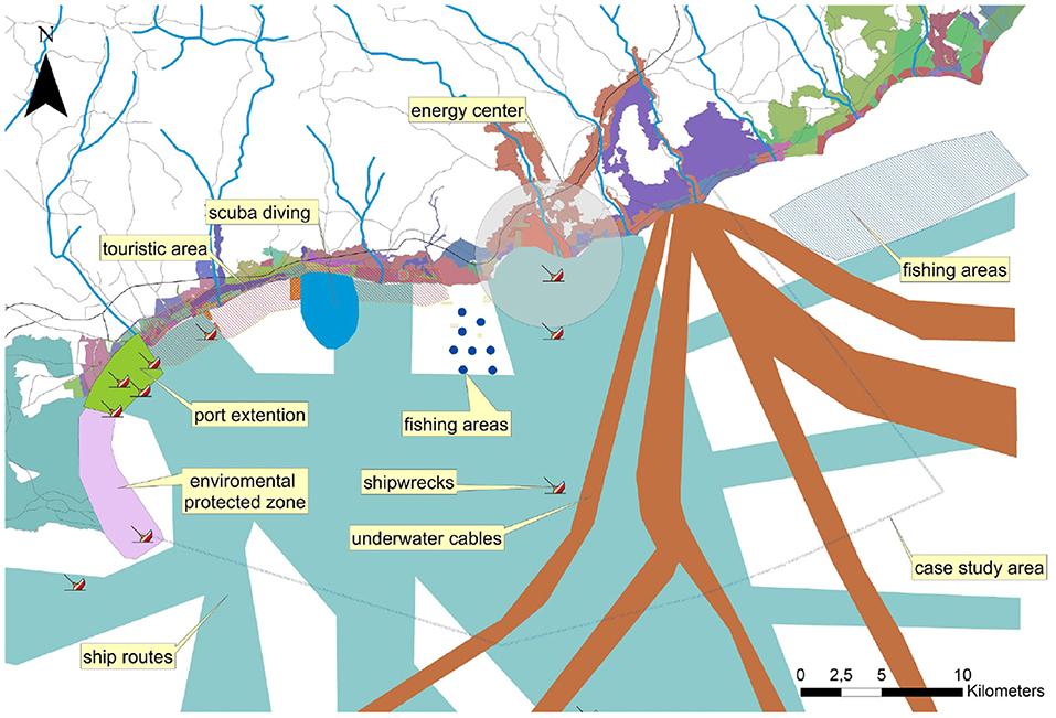
Figure 1. Real MSP map (Hadjimitsis et al., 2016).
To implement these approaches and applications, however, most of them have relied upon raster data structure using regular grid cells, principally due to its simplicity and ease of assessing spatial relationships among land grids, such as proximity and adjacency. Except for Stewart et al. (2004), Chandramouli et al. (2009), Cao and Ye (2013), Masoomi et al. (2013), little has been done utilizing vector data for decision-making units in MSP.
All the above-mentioned MSP problems were addressed initially by using heuristics or simpler approaches in the field of GIS with map crossings and weighting criteria (Pressey et al., 1993, 1997; Triana et al., 2019). However, later, they were formulated as mixed-integer/integer linear programs (MILP/ILP) in the framework of the set covering problem (SCP) and maximal covering problem (MCP) (Toregas and Revelle, 1973; Church and ReVelle, 1974; Kirkpatrick, 1983; Cocks and Baird, 1989; Underhill, 1994; Church et al., 1996; Williams and ReVelle, 1997; Possingham et al., 2000; Polasky et al., 2001). On the one hand, the most important advantage of using MILP/ILP to design MSP is that it can provide a globally optimal solution. On the other hand, an important disadvantage of them is related to the problem-solving computing time, which is very likely has a direct correlation with the data size and complexity (O'Hanley, 2009).
Apart from all of the above mentioned, despite many research papers dealing with MSP, the problem is yet to be concise, as for each actor, many technological, spatial, economic, environmental, and social objectives along with constraints must be addressed which are generally incompatible. Integrated into the optimum zoning of these criteria, mathematical models must be more advanced and computationally demanding than SCP and MCP formulations. To do so, Multiple Objective Mathematical Programming (MOMP) is applied to solve Mathematical Programming problems with more than one objective function. Given that usually, there is no unique optimal solution (optimizing all objective functions simultaneously), the aim is to find the most preferred among the Pareto optimal solutions (Deming, 1991).
To do so efficiently, MOMP methods have to combine optimization with decision support. To address this issue, the solution process can be divided into two separate phases: The first is the Pareto optimal solutions generation (all or a subset of them). The second is the subsequent involvement of the decision-maker if all the information is available (the so-called multi-criteria decision-making process).
Available procedures for these two phases are usually classified into three approaches (Cohon and Marks, 1975; Chiandussi et al., 2012), depending on whether the decision-maker is involved before, during, or after the search: a priori, interactive, and a posteriori approaches. In MOMP, a posteriori method is the most computationally demanding category among the other approaches. However, thanks to the enormous growth in calculation speed and advancement of Mathematical Programming methods, a posteriori method has become more attractive among today's decision-makers. Although the optimal solutions of these formulations are economically efficient, they usually lack spatial criteria. Spatial criteria may take a variety of forms (Williams and Snyder, 2005; Haight and Snyder, 2009).
Most commonly used criteria include compactness and connectivity (Wright et al., 1983; Fischer and Church, 2003; Önal and Briers, 2003; Tóth and McDill, 2008; Jafari and Hearne, 2013), proximity of selected sites (Rothley, 1999; Briers, 2002; Nalle et al., 2002; Önal and Briers, 2002; Ruliffson et al., 2003; Williams, 2008; Miller et al., 2009; Dissanayake et al., 2012), habitat fragmentation (Önal and Briers, 2002, 2005), contiguity (Cova and Church, 2000; Williams, 2002; Cerdeira and Pinto, 2005; Önal and Briers, 2006; Marianov et al., 2008; Önal and Wang, 2008; Tóth et al., 2009; Cerdeira et al., 2010; Duque et al., 2011; Carvajal et al., 2013; Jafari and Hearne, 2013), existence of buffers and corridors (Williams and ReVelle, 1996, 1998; Williams et al., 2005; Conrad et al., 2012), and accessibility (Ruliffson et al., 2003; Önal and Yanprechaset, 2007).
Among the most recent contributions, Cheng et al. (2015) presented two MPA spatial zoning models based on MOILP: a buffer cells model (BCM) and an external border cells model (EBCM). These models provide multi-objective zones for MPA planning that satisfy multiple conservation goals while ensuring optimal results. The EBCM has been selected for comparison with Marxan with zones because both of them ignore buffer cells. In summary, the EBCM holds several advantages over Marxan with zones for MPA spatial zoning. It guarantees optimality conditions, while providing a compactness/cost trade-off, in which decision-makers can explore according to their preferences. A procedure to solve trans-boundary water conflicts in the Gaunting reservoir basin based on the theory of a hybrid game and mathematical planning model has been developed by Zeng et al. (2019) to optimize use of water and pollutant discharge while maximizing net aggregate benefit and reduce water supplies and pollution prevention costs. A connectivity-based technique was employed to create the marine protected area networks by Fox et al. (2019) for multi-objective optimizing. In order to get the Pareto optimum set for networks up to 100 websites, the authors created a meta-heuristic Algorithm examined two marine realistic networks. Zhao et al. (2019) explored the conflicts between the development and exploitation of the marine area and ecological conservation using the Ecosystem Service Value Calculation (ESV). The results illustrate the advantages of optimization of the use of the sea area (Dengsha estuary area). They can tackle the multi-sector conflict problem and provide a fresh design for optimizing the spatial layout.
Based on the literature review, the main contributions of this paper can be summarized as follows:
• Problem definition: Since one of the main issues in MSP is to locate and allocate an optimal zone for a new human activity while considering the other existing activities, we define and describe a new problem in the scope of zoning in MSP,
• Problem formulation: Given the current state of the art, the most common approach is based on non-linear multi-objective models, which are usually solved using stochastic search algorithms, resulting in sub-optimal solutions. We choose to work on raster data, and hence our contribution is to formulate an exact linear model as a MOILP which aims at maximizing the interest of the area of the zone dedicated to one actor, while maximizing its spatial compactness.
• Problem resolution: To solve this model and determine the optimal solution, we use two resolution methods: WS (a weighted sum of the objectives) and AUGMECON2 (an interactive approach based on the classical ϵ-constraint method). Due to a very large number of integer variables and constraints in this MOILP model, we improve its resolution by using buffering techniques in a preprocessing phase.
• Experimental validation: We generate a set of artificial datasets to validate the approach and study both the sensitivity of the resolution methods and computation times with respect to various parameters.
The literature review shows among other things that MSP requires formal tools to assist the decision process and converge to an overall sustainable plan for the use of marine resources. As already said, in this work, we focus on the zoning problem, a specific sub-problem of MSP where a certain number of human activities already exist in a given marine area, and for which the optimal location of a new activity must be determined. The existing activities in the area are considered fixed and cannot be modified. The overall interest of the location of the new activity depends on a map, which is given for the whole area and represents the degree to which it is worthwhile or unattractive to carry out the activity at each point in the area.
The existing activities in the area can be classified into 3 categories:
• Shipping lanes (also called sea lanes or sea routes), which are regularly used navigable routes for large ships, and which cannot intersect with the new activity. These shipping lanes could also represent underwater cables for example,
• Ports (also called harbors), which are placed at the edge of the ocean (on the mainland), and are used for ships to load and unload their cargo or passengers,
• Restricted areas in the ocean, which represent other activities and which cannot intersect with the new activity. These restricted areas can, for example, represent marine protected areas, wind or tidal turbine farms, recreational areas, military areas, etc.
Next to that, the precise location of the new activity does not only depend on the interest map but also the distance to the various elements of the three categories of existing activities. Generally speaking, in this problem, we are going to impose the constraints of minimum and the maximum distance of the new activity to the different existing activities. In other words, the new activity should be located:
• At a minimum distance of each of the existing activities (depending on each existing activity),
• At a maximum distance of each of the existing activities (depending on each existing activity).
Finally, in our problem it is preferable that the zone for the new activity is as compact as possible, to avoid potential conflicts with new activities that may emerge in the area in the future.
The objective of this problem is therefore to determine the optimal location of the new activity that maximizes both its interest and its compactness. Meanwhile, it is to respect certain constraints of minimum and maximum distances to existing activities (and therefore without overlapping with them).
Figure 2 illustrates on a fictive maritime area this problem definition and its various elements. The upper dark gray part (with the topographic isolines) of the figure represents the mainland, on which 4 ports are located. The lower part represents the maritime area, in which the new activity (e.g., a fishing activity) has to be located, and in which various existing activities are already located: multiple shipping lanes, a windmill farm (restricted area), and a protected natural area (restricted area). The interest for the new activity is represented on the background map in 3 levels of gray (the more interesting the area, the darker it is). In this problem, the new activity has to be located at a given minimum distance of the shipping lanes (), at a given minimum and a given maximum distance of the closest port ( and ), as well as at a given minimum distance of restricted areas (). Three areas for the new activity are presented in the figure. A is located in a part of the sea that is quite interesting for the new activity. B on the other hand is located in a less interesting part, while C is located in a part of the maritime area that is very interesting. This average interest of the three areas is represented by the star rating (1 star corresponds to a low interest, 3 stars to a high interest). Next to that, each of these 3 areas has different compactness evaluations: B is very compact, as it is a rectangle, A is moderately compact, whereas C is not very compact. This compactness is represented by the squares rating on the figure. Choosing between these 3 areas, solely on basis of their compactness and their interest is already a difficult problem, as none of the areas dominates the other ones on both measures. Next to that, the figure also represents some of the distance constraints. For example, area A checks all the minimal distance constraints, whereas B violates a maximal distance constraint to the closest port () and a minimal distance to the restricted windmill farm (). Finally, area C violates the minimal distance constraint with respect to the shipping lane (). As a consequence, due to these constraints violations, B and C cannot be considered for this new activity, and only the area A is acceptable.
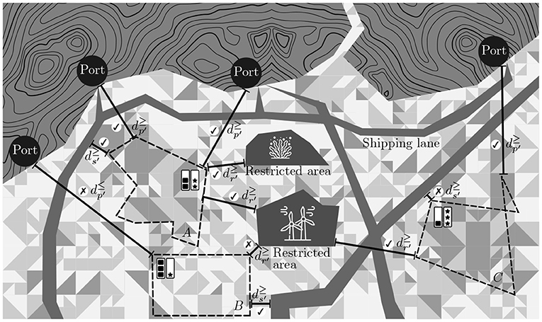
Figure 2. Problem definition.
As mentioned in section Problem Definition, the starting point of the problem at hand is geospatial data, which represent data related to or containing information about locations on the Earth's surface. In this work, we use raster data presented as a regular grid of cells or pixels. Each pixel in a raster has a value, which represents some unit of measurement about the underlying geographical area. The quality of raster data mainly varies depending on its resolution.
The top-left square of Figure 3 shows a satellite image. The associated raster data could for example represent the vegetation density in each of the pixels. As shown in the top-right grid, the resolution chosen for this example is 1 meter per pixel. The value contained in each of the elements of the raster grid corresponds to an average density measure of the vegetation in each of the cells. It is also possible to assign a color (bottom-right) to each of the cells, through a legend (bottom-left).
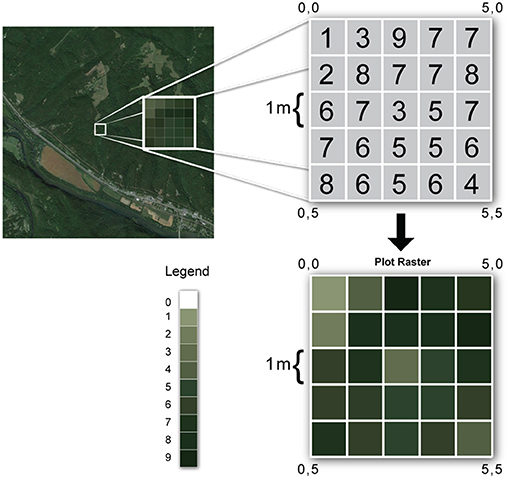
Figure 3. Raster concept (Laurini and Thompson, 1992).
Consequently, we assume that the interest map for the new activity is given by a two-dimensional matrix of uniform cells on a regular grid with nrow rows and ncol columns, resulting in nrow·ncol = m total cells. Each cell of this grid is assumed to have a homogeneous interest value for the given activity. Let be the set of cells of this grid.
Following the problem definition, let be the set of nl shipping lanes, which are represented as a set of cells on the raster grid. Let be a set of np ports, which are represented as a set of cells . Finally, let be a set of nr restricted areas (with which the new activity cannot intersect), which are represented as a set of cells .
Next to that, in order to keep an interactive process with the various stakeholders involved in the zoning problem, we will not only look for one optimal area for the new activity but also keep a record of other possibilities, so that the final choice is left to the decision-makers. The optimization algorithm should therefore output a number of possible areas for the new activity (which we will call the solutions of the optimization problem). Each solution is built around a central cell, to which adjacent cells are assigned in order to build the solution areas.
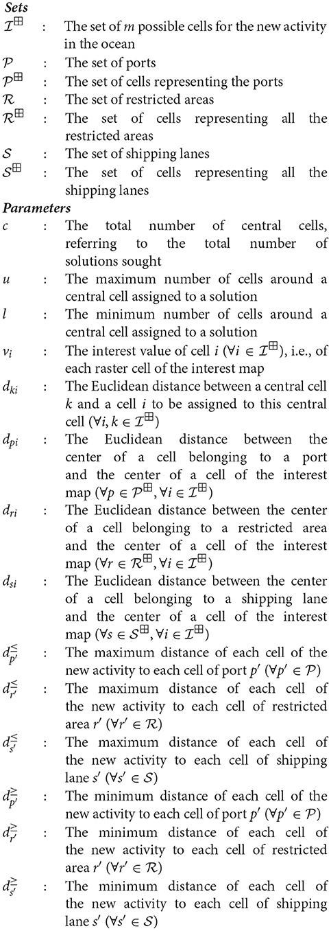
Before presenting the formal mathematical formulation, the notations associated with sets, input parameters, and decision variables are summarized as follows:
Decision Variables
Objectives:
Subject to:
Objective function (3) maximizes the total interest of a solution. Objective function (4) minimizes the sum of distances from individual cells in each solution to the central cell of that solution. As a consequence, a solution for the new activity is as compact and as contiguous as possible through this objective.
Constraint (5) ensures that exactly c central cells (i.e., solutions) are selected for the new activity. Constraint (6) guarantees that if cell k is selected as a central cell, i.e., xkk = 1, then up to a total of u other cells can be assigned to the solution formed around cell k. Constraint (7) expresses a similar concept as constraint (6), except that it defines the minimal size of a solution. Constraint (8) states that each cell can belong at most to one solution. Constraints (9), (11), (13) ensure that a solution is not located further than a maximum distance from each port, restricted area, and shipping lane. Similarly, constraints (10), (12), (14) guarantee that a solution is not located closer than a minimal distance from each port, restricted area, and shipping lane.
To solve the proposed multi-objective integer linear program, we study in this article two approaches for multi-objective optimization to achieve the appropriate exact Pareto front: first, an a priori method considering the weighted sum of the two objectives as a single objective function, and second, an a posteriori method using an improved version of the classical ϵ-constraint method (called AUGMECON2 by Mavrotas and Florios, 2013).
Before trying to solve the program for various problem sizes, it is worth noticing that inequations (9) to (14) generate a huge number of constraints involving a large number of integer variables. More precisely, each of these inequations renders m3 constraints related to m2 integer variables, where m = nrow·ncol. As an example, for a map with a resolution of 100 cells by 100 cells, this already amounts to 1012 constraints and 108 integer variables.
To overcome this difficulty, we propose to solve the problem using a two-step approach:
1. Reduce the feasible region for the mathematical program by removing regions where no solution can be found with a “buffer” technique presented below,
2. Remove the distance constraints (9) to (14) from the program and solve it using one of the two previously mentioned techniques.
A buffer is an area around a geographic feature containing locations that are within a specified distance of the feature (Laurini and Thompson, 1992; Jensen and Jensen, 2012). We use the concept of buffer to model the minimal and maximal distance constraints (9) to (14).
On the one hand, constraints (10), (12), and (14) are used to guarantee that a solution is not located too close to existing ports, activities, or shipping lanes. If we think in terms of a feasible region for the new activity on the interest map, these constraints imply that these ports, activities, and shipping lanes should be removed from this region, as well as the buffers around them, whose radiuses are given by the , , and parameters.
Constraints (9), (11), and (13) on the other hand guarantee that a solution is not located too far from these existing elements. Again, in terms of the feasible region for the new activity, this amounts to removing parts which are located outside of a buffer around the ports, activities, or shipping lanes, whose radiuses are given by the , , and parameters.
Figure 4 presents an illustrative example from section Problem Definition for which the buffer methodology has been applied to the central restricted area. The two white areas of the image represent parts of the feasible region for the new activity which have been removed because of two distance constraints involving that specific area [a minimal (12) and a maximal (11) constraint]. As a consequence, the solutions B and C are no longer feasible solutions, as they are not located totally inside the remaining feasible region. The same procedure is applied to other areas, ports, and shipping lanes until the final feasible region is identified.
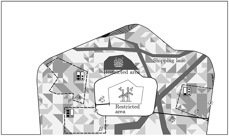
Figure 4. Modification of the feasible region by the buffering technique.
Once the reduction of the feasible region is performed through this buffering technique, the simplified mathematical program (without the distance constraints) can be solved either using the weighted sum or the AUGMECON2 technique.
The first resolution method that we study in this work uses a linear combination of the two objectives (3) and (4). The new objective therefore becomes :
where λ ∈ [0, 1] is a parameter. If λ = 0, then only the compactness objective is considered, and if λ = 1, then only the interest objective is used.
The second resolution method used in this study is AUGMECON2 (Mavrotas and Florios, 2013). It is an improvement of the original ϵ-constraint method which is along with the previously presented weighted sum method one of the two most popular resolution methods for solving multi-objective integer linear programs. It allows to generate representations of the Pareto front, which is the set of non-dominated solutions. As mentioned in Mavrotas (2009) the ϵ-constraint method, along with its improvements, has certain advantages in relation to the weighted sum method especially in case of discrete variables. AUGMECON2 compared to the ϵ-constraint method reduces the computation time during the generation of the points of the Pareto front by avoiding many redundant iterations.
In order to validate the proposals and to study their behavior when confronted with data, we propose to answer three questions:
• Are the mathematical model and the resolution methods able to find the optimal solution (validity)?
• How do the parameters of the resolution methods influence the solution (sensitivity)?
• How do the resolution methods compare w.r.t. to calculation times (complexity)?
To answer these three questions, we first propose a spatial data generator, which is able to generate artificial datasets with different characteristics (in terms of interest maps, number, and types of shipping lanes, ports, restricted areas, etc.). Then, the experimental protocol will be presented followed by the results.
Without loss of generality, we generate geospatial raster data for which the “bottom row” and the “right column” of the raster grid are considered as the mainland. This can be seen in Figure 5, where this mainland is represented by the dark gray cells containing no letters and no numbers.
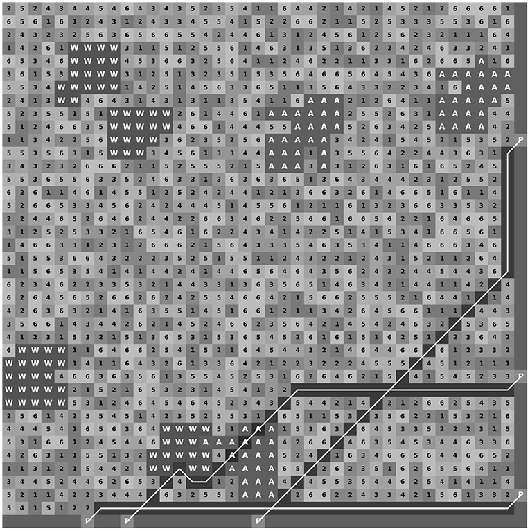
Figure 5. A sample data.
Consequently, all the rest of this data is the maritime area, in which the new activity has to be located. Each cell of this maritime area contains an interest value which indicates to what extend it is interesting to locate the new activity in that cell. This is depicted in Figure 5 by the 6 levels of gray associated with 6 levels of interest (1 corresponding to the less interesting cells, and 6 to the most interesting ones).
Let np be the number of ports to be generated for a given dataset. For generating these ports, we simply randomly select np cells from the mainland cells. In Figure 5, this is represented by the light gray cells marked with a white “P” on the mainland.
The restricted areas are contiguous areas in the maritime area, in which the new activity cannot be located. To generate one such area, we first select randomly a cell in the maritime area (the centroid). Then, we choose randomly cells from the adjacent cells of the centroid and assign them to the restricted area under construction. We then pick randomly cells from the adjacent cells of these cells, and repeat this process iteratively, until the size of the area is equal to the required size.
For our data, we are considering two types of restricted areas: restricted areas which allow shipping lanes to cross them (e.g., marine protected areas, fishing areas, etc.), and restricted areas which do not allow for intersections with routes (e.g., windmill farms, islands, etc.). For simplicity's sake, we will call the first type of restricted areas “protected areas”, label them “A” on Figure 5, whereas we will call the second type of restricted areas “windmill farms” and label them “W” on Figure 5. Let na be the number of protected areas and nw the number of windmill farms to be generated for a given dataset.
Let ns be the number of shipping lanes to be generated. Shipping lanes start and end in ports. To generate such a route, we use a shortest past algorithm, which is an adaptation of the A* algorithm (Hart et al., 1968). The algorithm generates the optimal route between an origin port and a destination port, while considering obstacles (the second type of restricted areas from above, labeled “W” on Figure 5) on the path. Figure 5 also shows 3 shipping lanes whose cells have been connected by a continuous white line.
Three types of interest maps have also been generated, as shown in Figure 6.
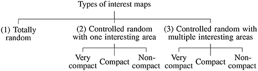
Figure 6. Different types of interest maps.
In the first approach called “Totally random”, a random integer interest value vi, vi∈{1, 2, 3, 4, 5, 6}, is assigned to each cell of the maritime area. In both “controlled” approaches, one or multiple interesting areas are fixed in the feasible region, by fixing vi to its maximum value (6). A representative method for the measurement of the compactness is called the Normalized Discrete Compactness (NDC) measure, suggested by Wenwen et al. (2013). The NDC approach has the advantage of being scale-invariant and can be applied when computing the compactness of shapes with holes on raster datasets. In each case, we choose to compare three degrees of compactness for those interesting areas which could be defined as:
• Very Compact: contiguous zone with no hole (0.5 < NDC)
• Compact: contiguous zone with one hole (0 < NDC ≤ 0.5)
• Not Compact: not contiguous zone with more than one hole (NDC ≤ 0).
The controlled datasets will obviously be used for validation purposes, whereas the random ones will contribute to study the differences between the different resolution methods, in terms of types of solutions, as well as in terms of complexity/calculation times. In total, this leads to the generation of 7 types of artificial datasets with respect to the interest map.
Next to that, regarding the ports, shipping lanes, protected areas and windmill farms, different sizes and configurations of those elements have also been generated, for each of the 7 types of interest maps. The data generation parameters are summarized in Table 1.
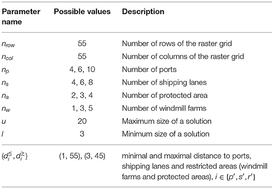
Table 1. Data generation parameters.
Regarding problem-specific parameters, we vary the minimal and maximal distance constraints to the different existing activities in the ocean as shown in Table 1. The total number of artificial datasets that have been generated are 7 × 33 × 2 = 1134.
The weighted sum resolution method requires one parameter to be fixed (λ) which gives the tradeoff between the two considered objectives. During some pre-tests we have checked on a sample of 21 datasets the effect of 11 different values (between 0 and 1) of the λ parameter on the weighted sum of the objectives, and we have determined that it varies linearly with λ. Consequently, for our more extended tests, we have considered that 3 values for λ are sufficient, which are shown in Table 2.
Table 2. Weighted sum parameter.
The AUGMECON2 parameters are configured in order to generate 3 optimal solutions of the Pareto front.
Multiple metrics could be recorded for each configuration of the algorithms and the following ones will be reported in the results section:
■ Computation times (separately for the buffering technique and the optimization part)
■ Location of the optimal solution
■ Characteristics of the optimal solution
• Compactness
• Number of cell candidates.
To address the first question about validation, the algorithms are run with their different parameter configurations on the controlled random datasets. For each run and each dataset, we check if the obtained solution is equal to or included in the (or one of the) artificially generated best locations of the interest maps.
Then, to answer the sensitivity question, we use the totally random datasets. We first measure the compactness of the solutions with respect to the variations of the algorithms' parameters, as well as the influence of the distance parameters on the compactness. Then, we compare the outputs of the algorithms to check if they produce the same or different solutions. In the second case, we also check if the solutions are intersecting, included one in the other, or totally disjoint. The effect of the distance parameters is also studied on the compactness of the solutions and their sizes.
Finally, to answer the complexity question, we evaluate the effect of the distance parameters on the resolution methods, by separating the buffer generation time from the optimization time.
The MOILP model is implemented in Python, version 3.8, by using the PuLP module, an LP modeler written in Python which calls an optimization software tool (CPLEX) as a solver. All experimental tests are implemented on a laptop with AMD Ryzen 5 PRO 2500u w/ Radeon Vega Mobile GFX 2.598GHZ processor with 16 GB RAM running Linux/Ubuntu 20.04.1 LTS.
In order to support the conclusions presented in this paper, statistical tests have been carried out to assess the significance of the results. More specifically, a Fisher-Snedecor procedure has been systematically done to evaluate the difference between the various sub-samples. All presented results are significant at a 95% level of confidence.
Having done all tests concerning validation, sensitivity analysis, and computation time, the main results can be summarized as follows:
■ Validation : (On controlled data) As mentioned before, to prove the validity of the model, we need to show if 100% of the achieved solution is equal to or encompasses the (or one of the) artificially generated best locations of the interest maps by using the controlled random areas. With regards to different types of interest maps for controlled datasets mentioned in Figure 6, we selected three of them as examples to show how the validity is approved; very compact and compact controlled random with one interesting area, and non-compact of that with multiple interesting areas. Figure 7 shows the geospatial raster-based map in which, in the maritime area, the controlled random area and optimal solution are displayed with white and dark gray raster cells. As can be seen, the white cells belong to both the optimal zone and a part of the controlled random area, and the other two dark gray cells complete the rest of this random area. Because of two holes in the controlled area, we define it as a “not very compact” area. Generally speaking, the total optimal solution is encompassed by the controlled area, that is, the optimal solution is exactly inside of that area. The other example is referred to as a very compact controlled random area, which is illustrated in Figure 8. Same as before, the white cells not only represent a part of a very compact controlled area but also the optimal solution, in which except for two dark gray cells of the controlled area, the others are inclusively selected. And the last example is for the non-compact controlled area shown in Figure 9. In this figure, three different non-compact controlled areas are generated, and the optimal zone has been selected as one of them. It is worth noticing that in all three cases, the model returns not only a compact solution but also the most interested one. By doing so, according to the tests, we can generally conclude that the obtained solution is %100 equal to or included in the controlled random generated zone.
■ Sensitivity Analysis : (On the random data)
1. Compactness:
• The compactness measure has been averaged over all configurations for the two different levels of buffers. First, by increasing the λ for WS, the weight of the interest function is growing while that of compactness is decreasing. This is why, in the given results, the larger the λ, the less compact solutions are achieved. Figure 11 shows the relationship between the compactness of solution and the algorithm parameters, in which WS has a downward tendency from compact to non-compact solutions by increasing the λ. Regarding AUGMECON2, the sensitivity to the compactness constraint is different. Figure 10 highlights an example of Pareto-optimal solutions yield by AUGMECON2 method to show the convergence of two objective functions.
The objective function (4) is related to the minimum distance between the center cell of the solution and the candidate cells around it. As can be seen in Pareto-front (Figure 10), by increasing this objective function (4) which is shifted into constraints, we are relaxing this constraint and going toward the maximum value of the objective function (3) which represents the interest. However, since the algorithm has to satisfy both objective functions at the same time, it tries to return different shapes by keeping nearly the same compactness, instead of giving less compact solutions. Therefore, the more objective function(4) (solution), the less the variability, illustrated in Figure 11. And on the other hand, by increasing the objective (4), the focus of the algorithm goes on the maximum interest value by selecting more and more cells, but the size constraint, which has the maximum value, will impose another limitation on the algorithm to find fewer various solutions with different compactness.
2. Number of candidate cells: Figure 12 reports that the average number of candidate cells of the solution for WS does not depend on the buffer size, while AUGMECON2 is impacted by the buffer. A larger buffer size decreases the number of candidate cells returned by the algorithm. These conclusions are supported by significant statistical tests (p < 0.05). One possible explanation is the fact that the difference between the two considered buffers is not large enough to globally impact the number of candidate cells of WS while AUGMECON2 is very sensitive to the buffer and the solution space.
■ Computation Time : (On the random data)
1. The total computational time is calculated by the summation of the optimization and buffer time. Figure 13 pinpoints the difference between WS and AUGMECON2 total computational time. As shown, for a smaller feasible area (i.e., larger buffer size), MOILP model is solved in a shorter time for both WS and AUGMECON2 rather than for a larger solution space (i.e., smaller buffer size). With a smaller buffer, we observe a more important computation time for AUGMECON2 (p < 0.05). However, thanks to its sensitivity to the buffer size, AUGMECON2 becomes more efficient with a larger buffer (p < 0.05).
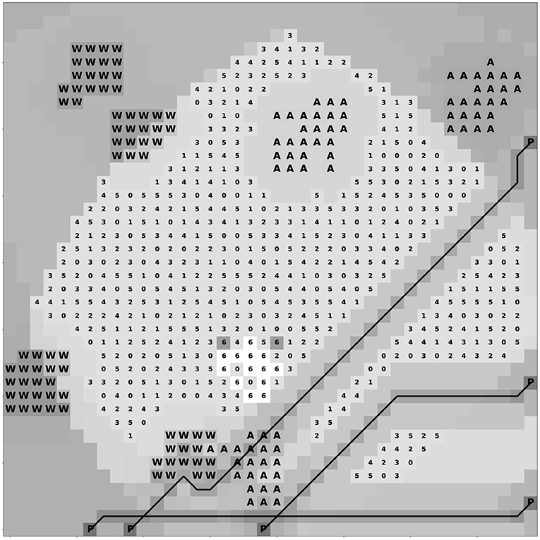
Figure 7. The sample validity map with one compact area.
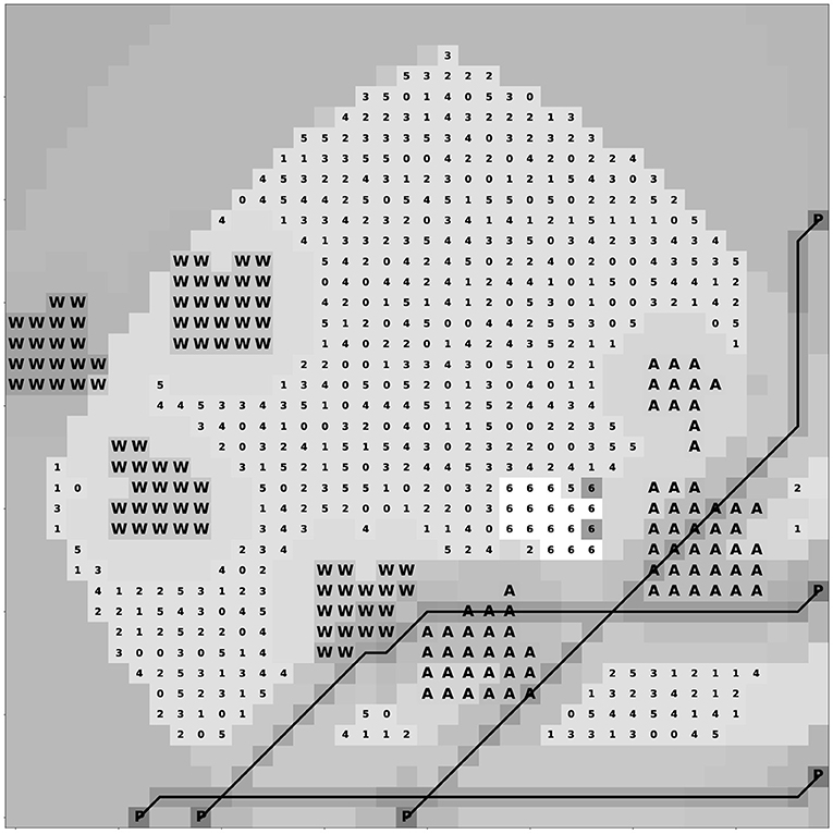
Figure 8. The sample validity map with one very compact area.
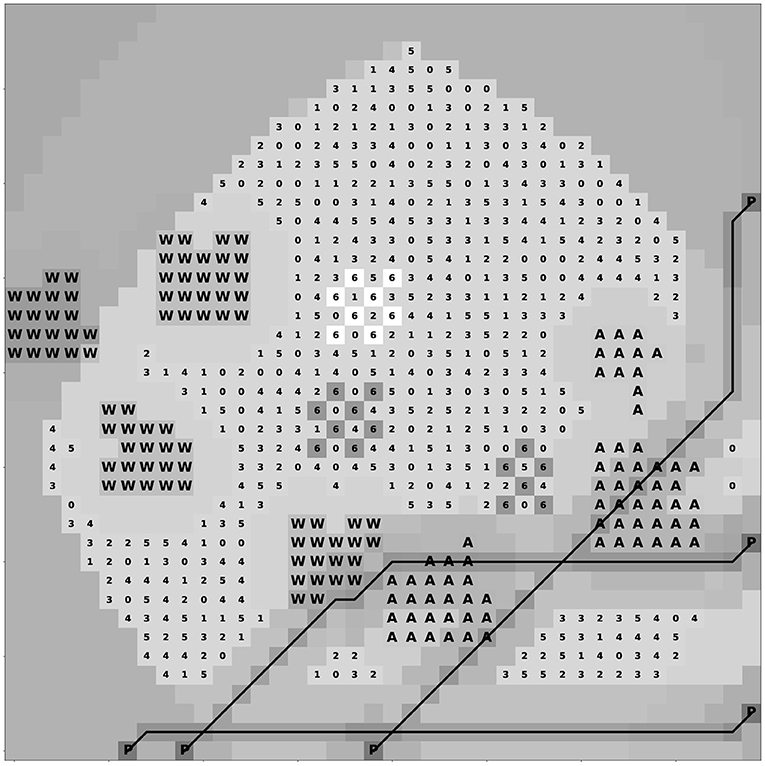
Figure 9. The sample validity map with multiple non-compact areas.
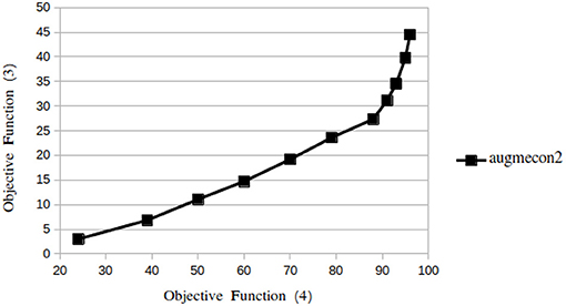
Figure 10. The Pareto Front.
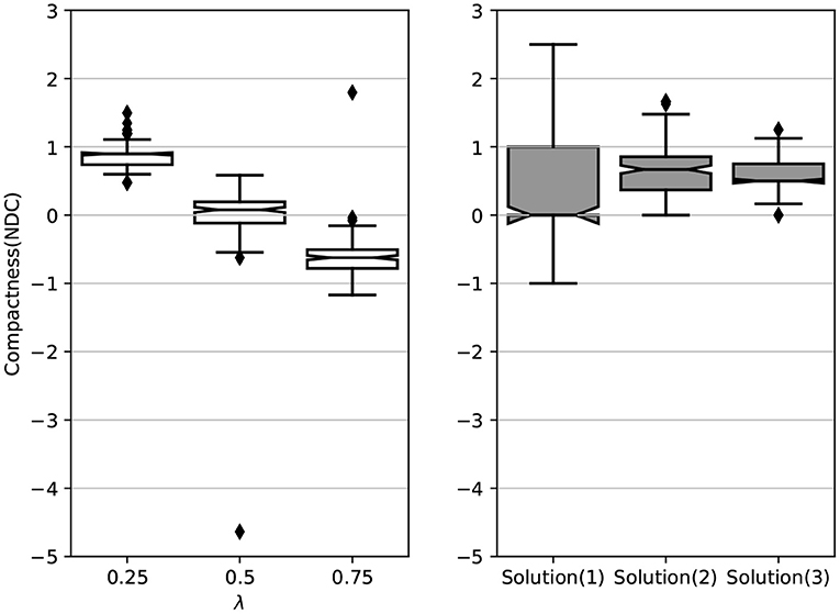
Figure 11. Average Compactness for 3 Pareto-optimal solutions of AUGMECON2 with increasing the objective function 4 and that of WS w.r.t λ.
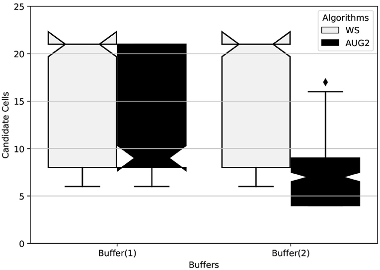
Figure 12. The average candidate cells of all configurations for each buffer.
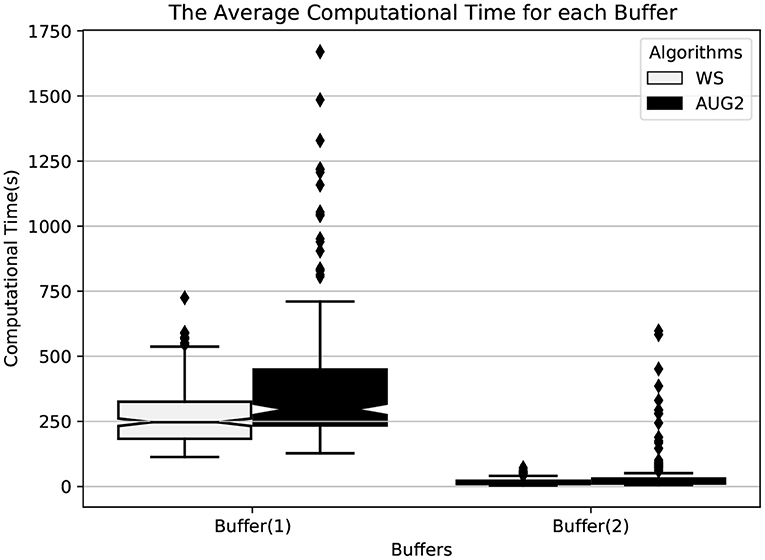
Figure 13. Average time of all configurations for each buffer.
In this paper, a novel multi-objective mathematical model is proposed to solve the problem of locating and allocating a new human activity optimally in a given marine area. The proposed approach highlights an exact resolution of the problem. To solve it, we analyzed two resolution methods, a weighted sum of the objectives and AUGMECON2, an enhanced version of the classical ϵ-constraint method. An empirical study based on synthetic data proves the ability of both methods to yield optimal solutions.
Our study shows also that AUGMECON2 represents the most promising approach in terms of relevance and diversity of the solutions, compactness, and computation time. Indeed, AUGMECON2 is able to exploit almost every run to produce a different solution. It also offers the possibility to easily control the number of generated solutions. On the opposite, WS provides less balanced solutions between the two objectives of interest and compactness while being less sensitive to the buffering technique.
Among the perspectives of this work, the next challenge is to scale up the problem resolution to be able to solve larger problems. This objective is being achieved through current work developing meta-heuristics that are faster while providing solutions that are close to optimality. To be more compatible with reality, another extension of this work would concern the determination of the best location for multiple new activities at the same time. In case of conflicts, we plan on proposing some negotiation-based algorithms to reach a compromise solution satisfying all actors.
The raw data supporting the conclusions of this article will be made available by the authors, without undue reservation.
MB, RB, PM, and EB contributed to the conception, design of the study, and wrote sections of the manuscript. MB implemented the models, generated the data, and wrote the first draft of the manuscript. MB, RB, and PM performed the statistical analysis. All authors contributed to manuscript revision, read, and approved the submitted version.
The authors declare that the research was conducted in the absence of any commercial or financial relationships that could be construed as a potential conflict of interest.
All claims expressed in this article are solely those of the authors and do not necessarily represent those of their affiliated organizations, or those of the publisher, the editors and the reviewers. Any product that may be evaluated in this article, or claim that may be made by its manufacturer, is not guaranteed or endorsed by the publisher.
Abspoel, L., Mayer, I., Keijser, X., Warmelink, H., Fairgrieve, R., Ripken, M., et al. (2019). Communicating maritime spatial planning: the MSP challenge approach. Mar. Policy 2019:103486. doi: 10.1016/j.marpol.2019.02.057
Aerts, J. C., Eisinger, E., Heuvelink, G. B., and Stewart, T. J. (2003). Using linear integer programming for multi-site land-use allocation. Geograph. Anal. 35, 148–169. doi: 10.1111/j.1538-4632.2003.tb01106.x
Agardy, T. (2010). Ocean Zoning: Making Marine Management More Effective. London: Routledge. doi: 10.4324/9781849776462
Agardy, T. S. (2015). “Marine protected areas and ocean planning,” in Routledge Handbook of Ocean Resources and Management, eds H. D. Smith and J. Luis (London: Routledge; Springer), 476–492. Available online at: https://www.taylorfrancis.com/chapters/edit/10.4324/9780203115398-32/marineprotected-areas-ocean-planning-tundiagardy
Airame, S. (2005). Channel Islands National Marine Sanctuary: Advancing the Science and Policy of Marine Protected Areas. Place Matters: Geospatial Tools for Marine Science, Conservation, and Management in the Pacific Northwest. Oregon State University Press, Corvallis, OR, 91–124.
Borges, R., Eyzaguirre, I., Barboza, R. S. L., and Glaser, M. (2020). Systematic review of spatial planning and marine protected areas: a Brazilian perspective. Front. Mar. Sci. 7:499. doi: 10.3389/fmars.2020.00499
Briers, R. A. (2002). Incorporating connectivity into reserve selection procedures. Biol. Conserv. 103, 77–83. doi: 10.1016/S0006-3207(01)00123-9
Brodie, J., and Waterhouse, J. (2012). A critical review of environmental management of the “not so great” barrier reef. Estuar. Coast. Shelf Sci. 104, 1–22. doi: 10.1016/j.ecss.2012.03.012
Cao, K., and Ye, X. (2013). Coarse-grained parallel genetic algorithm applied to a vector based land use allocation optimization problem: the case study of tongzhou newtown, Beijing, China. Stochast. Environ. Res. Risk Assess. 27, 1133–1142. doi: 10.1007/s00477-012-0649-y
Carvajal, R., Constantino, M., Goycoolea, M., Vielma, J. P., and Weintraub, A. (2013). Imposing connectivity constraints in forest planning models. Operat. Res. 61, 824–836. doi: 10.1287/opre.2013.1183
Cerdeira, J. O., and Pinto, L. S. (2005). Requiring connectivity in the set covering problem. J. Combinat. Optimizat. 9, 35–47. doi: 10.1007/s10878-005-5482-5
Cerdeira, J. O., Pinto, L. S., Cabeza, M., and Gaston, K. J. (2010). Species specific connectivity in reserve-network design using graphs. Biol. Conserv. 143, 408–415. doi: 10.1016/j.biocon.2009.11.005
Chandramouli, M., Huang, B., and Xue, L. (2009). Spatial change optimization. Photogrammetr. Eng. Remote Sens. 75, 1015–1022. doi: 10.14358/PERS.75.8.1015
Cheng, H.-C., Château, P.-A., and Chang, Y.-C. (2015). Spatial zoning design for marine protected areas through multi-objective decision-making. Ocean Coastal Manage. 108, 158–165. doi: 10.1016/j.ocecoaman.2014.08.018
Chiandussi, G., Codegone, M., Ferrero, S., and Varesio, F. E. (2012). Comparison of multi-objective optimization methodologies for engineering applications. Comput. Math. Appl. 63, 912–942. doi: 10.1016/j.camwa.2011.11.057
Church, R., and ReVelle, C. (1974). “The maximal covering location problem,” in Papers of the Regional Science Association (Cham: Springer-Verlag), 101–118. doi: 10.1007/BF01942293
Church, R. L., Stoms, D. M., and Davis, F. W. (1996). Reserve selection as a maximal covering location problem. Biol. Conserv. 76, 105–112. doi: 10.1016/0006-3207(95)00102-6
Cocks, K., and Baird, I. A. (1989). Using mathematical programming to address the multiple reserve selection problem: an example from the Eyre peninsula, South Australia. Biol. Conserv. 49, 113–130. doi: 10.1016/0006-3207(89)90083-9
Cohon, J. L., and Marks, D. H. (1975). A review and evaluation of multiobjective programing techniques. Water Resour. Res. 11, 208–220. doi: 10.1029/WR011i002p00208
Conrad, J. M., Gomes, C. P., van Hoeve, W.-J., Sabharwal, A., and Suter, J. F. (2012). Wildlife corridors as a connected subgraph problem. J. Environ. Econ. Manage. 63, 1–18. doi: 10.1016/j.jeem.2011.08.001
Cova, T. J., and Church, R. L. (2000). Contiguity constraints for single-region site search problems. Geograph. Anal. 32, 306–329. doi: 10.1111/j.1538-4632.2000.tb00430.x
Dahl, R.Commission, I. O., et al. (2009). Marine Spatial Planning: A Step-by-Step Approach Toward Ecosystem-Based Management. Paris: UNESCO/IOC.
Day, J. C. (2002). Zoning-lessons from the great barrier reef marine park. Ocean Coast. Manage. 45, 139–156. doi: 10.1016/S0964-5691(02)00052-2
de Souza Rêgo, I., Aguiar, L. F. M. C., and de Oliveira Soares, M. (2016). Environmental zoning and coastal zone conservation: the case of a protected area in northeastern Brazil. Revista de Gest ao Costeira Integrada-Journal of Integrated Coastal Zone Management 16, 35–43. doi: 10.5894/rgci603
Deming, S. N. (1991). Multiple-criteria optimization. J. Chromatogr. A 550, 15–25. doi: 10.1016/S0021-9673(01)88527-7
Dissanayake, S. T., Önal, H., Westervelt, J. D., and Balbach, H. E. (2012). Incorporating species relocation in reserve design models: an example from ft. Benning Ga. Ecol. Modell. 224, 65–75. doi: 10.1016/j.ecolmodel.2011.07.016
Domínguez-Tejo, E., Metternicht, G., Johnston, E., and Hedge, L. (2016). Marine spatial planning advancing the ecosystem-based approach to coastal zone management: a review. Mar. Policy 72, 115–130. doi: 10.1016/j.marpol.2016.06.023
Douvere, F. (2008). The importance of marine spatial planning in advancing ecosystem-based sea use management. Mar. Policy 32, 762–771. doi: 10.1016/j.marpol.2008.03.021
Dudley, N. (2008). Guidelines for Applying Protected Area Management Categories. IUCN. doi: 10.2305/IUCN.CH.2008.PAPS.2.en
Duque, J. C., Church, R. L., and Middleton, R. S. (2011). The p-regions problem. Geograph. Anal. 43, 104–126. doi: 10.1111/j.1538-4632.2010.00810.x
Fernandes, L., Day, J., Lewis, A., Slegers, S., Kerrigan, B., Breen, D., et al. (2005). Establishing representative no-take areas in the great barrier reef: large-scale implementation of theory on marine protected areas. Conserv. Biol. 19, 1733–1744. doi: 10.1111/j.1523-1739.2005.00302.x
Fischer, D. T., and Church, R. L. (2003). Clustering and compactness in reserve site selection: an extension of the biodiversity management area selection model. Forest Sci. 49, 555–565. doi: 10.1093/forestscience/49.4.555
Foster, E., Haward, M., and Coffen-Smout, S. (2005). Implementing integrated oceans management: Australia's south east regional marine plan (SERMP) and Canada's eastern Scotian shelf integrated management (ESSIM) initiative. Mar. Policy 29, 391–405. doi: 10.1016/j.marpol.2004.06.007
Fox, A. D., Corne, D. W., Mayorga Adame, C. G., Polton, J. A., Henry, L.-A., and Roberts, J. M. (2019). An efficient multi-objective optimization method for use in the design of marine protected area networks. Front. Mar. Sci. 6:17. doi: 10.3389/fmars.2019.00017
Hadjimitsis, D., Agapiou, A., Themistocleous, K., Mettas, C., Evagorou, E., Soulis, G., et al. (2016). Maritime spatial planning in cyprus. Open Geosci. 8, 653–661. doi: 10.1515/geo-2016-0061
Haight, R. G., and Snyder, S. A. (2009). “Integer programming methods for reserve selection and design,” in Spatial Conservation Prioritization. Quantitative Methods and Computational Tools, A. Moilanen, K. A. Wilson, and H. Possingham (Oxford, UK: Oxford University Press), 43–57.
Halpern, B. S., McLeod, K. L., Rosenberg, A. A., and Crowder, L. B. (2008). Managing for cumulative impacts in ecosystem-based management through ocean zoning. Ocean Coast. Manage. 51, 203–211. doi: 10.1016/j.ocecoaman.2007.08.002
Hart, P. E., Nilsson, N. J., and Raphael, B. (1968). A formal basis for the heuristic determination of minimum cost paths. IEEE Trans. Syst. Sci. Cybernet. 4, 100–107. doi: 10.1109/TSSC.1968.300136
Jafari, N., and Hearne, J. (2013). A new method to solve the fully connected reserve network design problem. Eur. J. Operat. Res. 231, 202–209. doi: 10.1016/j.ejor.2013.05.015
Jensen, J. R., and Jensen, R. R. (2012). Introductory Geographic Information Systems. London: Pearson Higher Ed. Available online at: https://www.pearson.com/us/highereducation/program/Jensen-Introductory-Geographic-Information-Systems/PGM290591.html?tab=resources
Katsanevakis, S., Stelzenmüller, V., South, A., Sørensen, T. K., Jones, P. J., Kerr, S., et al. (2011). Ecosystem-based marine spatial management: review of concepts, policies, tools, and critical issues. Ocean Coast. Manage. 54, 807–820. doi: 10.1016/j.ocecoaman.2011.09.002
Kirkpatrick, J. (1983). An iterative method for establishing priorities for the selection of nature reserves: an example from Tasmania. Biol. Conserv. 25, 127–134. doi: 10.1016/0006-3207(83)90056-3
Korhonen, I. M. (1996). Riverine ecosystems in international law. Nat. Resour. J. 36:481. doi: 10.1163/15718109620294951
Laurini, R., and Thompson, D. (1992). Fundamentals of Spatial Information Systems, Vol. 37. Academic Press. doi: 10.1016/B978-0-08-092420-5.50014-1
Liffmann, R. H., Huntsinger, L., and Forero, L. C. (2000). To ranch or not to ranch: home on the urban range? Rangeland Ecol. Manage. 53, 362–370. doi: 10.2307/4003745
Ligmann-Zielinska, A., Church, R. L., and Jankowski, P. (2008). Spatial optimization as a generative technique for sustainable multiobjective land-use allocation. Int. J. Geograph. Inform. Sci. 22, 601–622. doi: 10.1080/13658810701587495
Lombard, A. T., Dorrington, R. A., Reed, J. R., Ortega-Cisneros, K., Penry, G. S., Pichegru, L., et al. (2019). Key challenges in advancing an ecosystem-based approach to marine spatial planning under economic growth imperatives. Front. Mar. Sci. 6:146. doi: 10.3389/fmars.2019.00146
Marianov, V., ReVelle, C., and Snyder, S. (2008). Selecting compact habitat reserves for species with differential habitat size needs. Comput. Operat. Res. 35, 475–487. doi: 10.1016/j.cor.2006.03.011
Masoomi, Z., Mesgari, M. S., and Hamrah, M. (2013). Allocation of urban land uses by multi-objective particle swarm optimization algorithm. Int. J. Geograph. Inform. Sci. 27, 542–566. doi: 10.1080/13658816.2012.698016
Masoudi, M., Centeri, C., Jakab, G., Nel, L., and Mojtahedi, M. (2021). GIS-based multi-criteria and multi-objective evaluation for sustainable land-use planning (case study: Qaleh Ganj County, Iran) “landuse planning using MCE and MOLA”. Int. J. Environ. Res. 15, 457–474. doi: 10.1007/s41742-021-00326-0
Mavrotas, G. (2009). Effective implementation of the ϵ-constraint method in multi-objective mathematical programming problems. Appl. Math. Comput. 213, 455–465. doi: 10.1016/j.amc.2009.03.037
Mavrotas, G., and Florios, K. (2013). An improved version of the augmented ε-constraint method (AUGMECON2) for finding the exact pareto set in multi-objective integer programming problems. Appl. Math. Comput. 219, 9652–9669. doi: 10.1016/j.amc.2013.03.002
Miller, J. R., Snyder, S. A., Skibbe, A. M., and Haight, R. G. (2009). Prioritizing conservation targets in a rapidly urbanizing landscape. Landscape Urban Plan. 93, 123–131. doi: 10.1016/j.landurbplan.2009.06.011
Nalle, D. J., Arthur, J. L., Montgomery, C. A., and Sessions, J. (2002). Economic and spatial impacts of an existing reserve network on future augmentation. Environ. Model. Assess. 7, 99–105. doi: 10.1023/A:1015697632040
Norse, E. A. (2010). Ecosystem-based spatial planning and management of marine fisheries: why and how? Bull. Mar. Sci. 86, 179–195. Available online at: https://www.ingentaconnect.com/content/umrsmas/bullmar/2010/00000086/00000002/art00004#expand/collapse
O'Hanley, J. R. (2009). Using the right tool to get the job done-recommendations on the use of exact and heuristics methods for solving resource allocation problems in environmental planning and management. Biol. Conserv. 142, 697–698. doi: 10.1016/j.biocon.2008.12.024
Önal, H., and Briers, R. A. (2002). Incorporating spatial criteria in optimum reserve network selection. Proc. R. Soc. Lond. Ser. B Biol. Sci. 269, 2437–2441. doi: 10.1098/rspb.2002.2183
Önal, H., and Briers, R. A. (2003). Selection of a minimum-boundary reserve network using integer programming. Proc. R. Soc. Lond. Ser. B Biol. Sci. 270, 1487–1491. doi: 10.1098/rspb.2003.2393
Önal, H., and Briers, R. A. (2005). Designing a conservation reserve network with minimal fragmentation: a linear integer programming approach. Environ. Model. Assess. 10, 193–202. doi: 10.1007/s10666-005-9009-3
Önal, H., and Briers, R. A. (2006). Optimal selection of a connected reserve network. Operat. Res. 54, 379–388. doi: 10.1287/opre.1060.0272
Önal, H., and Wang, Y. (2008). A graph theory approach for designing conservation reserve networks with minimal fragmentation. Networks Int. J. 51, 142–152. doi: 10.1002/net.20211
Önal, H., Wang, Y., Dissanayake, S. T., and Westervelt, J. D. (2016). Optimal design of compact and functionally contiguous conservation management areas. Eur. J. Operat. Res. 251, 957–968. doi: 10.1016/j.ejor.2015.12.005
Önal, H., and Yanprechaset, P. (2007). Site accessibility and prioritization of nature reserves. Ecol. Econ. 60, 763–773. doi: 10.1016/j.ecolecon.2006.01.011
Polasky, S., Camm, J. D., and Garber-Yonts, B. (2001). Selecting biological reserves cost-effectively: an application to terrestrial vertebrate conservation in oregon. Land Econ. 77, 68–78. doi: 10.2307/3146981
Possingham, H., Ball, I., and Andelman, S. (2000). “Mathematical methods for identifying representative reserve networks,” in Quantitative Methods for Conservation Biology, eds S. Ferson and M. Burgman (New York, NY: Springer), 291–306. doi: 10.1007/0-387-22648-6_17
Pressey, R., Humphries, C., Margules, C., Vane-Wright, R., and Williams, P. (1993). Beyond opportunism: Key principles for systematic reserve selection. Trends Ecol. Evol. 8, 124–128. doi: 10.1016/0169-5347(93)90023-I
Pressey, R., Possingham, H., and Day, J. (1997). Effectiveness of alternative heuristic algorithms for identifying indicative minimum requirements for conservation reserves. Biol. Conserv. 80, 207–219. doi: 10.1016/S0006-3207(96)00045-6
Rothley, K. (1999). Designing bioreserve networks to satisfy multiple, conflicting demands. Ecol. Appl. 9, 741–750. doi: 10.1890/1051-0761(1999)009[0741:DBNTSM]2.0.CO;2
Ruliffson, J. A., Haight, R. G., Gobster, P. H., and Homans, F. R. (2003). Metropolitan natural area protection to maximize public access and species representation. Environ. Sci. Policy 6, 291–299. doi: 10.1016/S1462-9011(03)00038-8
Russ, G. R., and Zeller, D. C. (2003). From mare liberum to mare reservarum. Mar. Policy 27, 75–78. doi: 10.1016/S0308-597X(02)00054-4
Sainsbury, K. J., Punt, A. E., and Smith, A. D. (2000). Design of operational management strategies for achieving fishery ecosystem objectives. ICES J. Mar. Sci. 57, 731–741. doi: 10.1006/jmsc.2000.0737
Santos, C. F., Ehler, C. N., Agardy, T., Andrade, F., Orbach, M. K., and Crowder, L. B. (2019). “Marine spatial planning,” in World Seas: An Environmental Evaluation, ed C. Sheppard (Coventry: Elsevier), 571–592. doi: 10.1016/B978-0-12-805052-1.00033-4
Shirina, N., and Parfenyukova, E. (2021). “Zoning the urban area on the basis of the principles and methods of GIS-mapping,” in Innovations and Technologies in Construction: Selected Papers of Buildintech BIT 2021 (Cham: Springer), 342–348. doi: 10.1007/978-3-030-72910-3_50
Smith, H. D., Maes, F., Stojanovic, T. A., and Ballinger, R. C. (2011). The integration of land and marine spatial planning. J. Coast. Conserv. 15, 291–303. doi: 10.1007/s11852-010-0098-z
Stewart, T. J., Janssen, R., and van Herwijnen, M. (2004). A genetic algorithm approach to multiobjective land use planning. Comput. Operat. Res. 31, 2293–2313. doi: 10.1016/S0305-0548(03)00188-6
Stojanovic, T., and Gee, K. (2020). Governance as a framework to theorise and evaluate marine planning. Mar. Policy 120:104115. doi: 10.1016/j.marpol.2020.104115
Strickland-Munro, J., Kobryn, H., Brown, G., and Moore, S. A. (2016). Marine spatial planning for the future: using public participation GIS (PPGIS) to inform the human dimension for large marine parks. Mar. Policy 73, 15–26. doi: 10.1016/j.marpol.2016.07.011
Taussik, J. (2007). The opportunities of spatial planning for integrated coastal management. Mar. Policy 31, 611–618. doi: 10.1016/j.marpol.2007.03.006
Toregas, C., and Revelle, C. (1973). Binary logic solutions to a class of location problem. Geograph. Anal. 5, 145–155. doi: 10.1111/j.1538-4632.1973.tb01004.x
Tóth, S. F., Haight, R. G., Snyder, S. A., George, S., Miller, J. R., Gregory, M. S., et al. (2009). Reserve selection with minimum contiguous area restrictions: an application to open space protection planning in suburban chicago. Biol. Conserv. 142, 1617–1627. doi: 10.1016/j.biocon.2009.02.037
Tóth, S. F., and McDill, M. E. (2008). Promoting large, compact mature forest patches in harvest scheduling models. Environ. Model. Assess. 13, 1–15. doi: 10.1007/s10666-006-9080-4
Triana, K. (2019). GIS developments for ecosystem-based marine spatial planning and the challenges faced in indonesia. ASEAN J. Sci. Technol. Dev. 36, 113–118. doi: 10.29037/ajstd.587
Trouillet, B. (2020). Reinventing marine spatial planning: a critical review of initiatives worldwide. J. Environ. Policy Plann. 22, 441–459. doi: 10.1080/1523908X.2020.1751605
Underhill, L. (1994). Optimal and suboptimal reserve selection algorithms. Biol. Conserv. 70, 85–87. doi: 10.1016/0006-3207(94)90302-6
Wenwen, L., Goodchild, F., and Church, R. (2013). An efficient measure of compactness for 2D shapes and its application in regionalization problems. Int. J. Geograph. Inform. Sci. 27, 1227–1250. doi: 10.1080/13658816.2012.752093
Williams, J., and ReVelle, C. (1996). A 0-1 programming approach to delineating protected reserves. Environ. Plann. B Plann. Design 23, 607–624. doi: 10.1068/b230607
Williams, J. C. (2002). A linear-size zero-one programming model for the minimum spanning tree problem in planar graphs. Networks Int. J. 39, 53–60. doi: 10.1002/net.10010
Williams, J. C. (2008). Optimal reserve site selection with distance requirements. Comput. Operat. Res. 35, 488–498. doi: 10.1016/j.cor.2006.03.012
Williams, J. C., and ReVelle, C. S. (1997). Applying mathematical programming to reserve selection. Environ. Model. Assess. 2, 167–175. doi: 10.1023/A:1019001125395
Williams, J. C., and ReVelle, C. S. (1998). Reserve assemblage of critical areas: a zero-one programming approach. Eur. J. Operat. Res. 104, 497–509. doi: 10.1016/S0377-2217(97)00017-9
Williams, J. C., ReVelle, C. S., and Levin, S. A. (2005). Spatial attributes and reserve design models: a review. Environ. Model. Assess. 10, 163–181. doi: 10.1007/s10666-005-9007-5
Williams, J. C., and Snyder, S. A. (2005). Restoring habitat corridors in fragmented landscapes using optimization and percolation models. Environ. Model. Assess. 10, 239–250. doi: 10.1007/s10666-005-9003-9
Wright, J., Revelle, C., and Cohon, J. (1983). A multiobjective integer programming model for the land acquisition problem. Region. Sci. Urban Econ. 13, 31–53. doi: 10.1016/0166-0462(83)90004-2
Yao, J., Zhang, X., and Murray, A. T. (2018). Spatial optimization for land-use allocation: accounting for sustainability concerns. Int. Region. Sci. Rev. 41, 579–600. doi: 10.1177/0160017617728551
Zeng, Y., Li, J., Cai, Y., Tan, Q., and Dai, C. (2019). A hybrid game theory and mathematical programming model for solving trans-boundary water conflicts. J. Hydrol. 570, 666–681. doi: 10.1016/j.jhydrol.2018.12.053
Zhao, P., Jin, S., and Kang, M. (2019). “Study on optimization of sea area utilization: a case study of Dengsha Estuary,” in 2019 2nd International Conference on Sustainable Energy, Environment and Information Engineering (SEEIE 2019) (Dordrecht: Atlantis Press), 153–156. doi: 10.2991/seeie-19.2019.35
Keywords: marine spatial planning, multi-objective integer linear optimization, buffering, interest, compactness, raster data
Citation: Basirati M, Billot R, Meyer P and Bocher E (2021) Exact Zoning Optimization Model for Marine Spatial Planning (MSP). Front. Mar. Sci. 8:726187. doi: 10.3389/fmars.2021.726187
Received: 29 June 2021; Accepted: 25 October 2021;
Published: 18 November 2021.
Edited by:
Robin Kundis Craig, University of Southern California, United StatesReviewed by:
Nicolaos Theodossiou, Aristotle University of Thessaloniki, GreeceCopyright © 2021 Basirati, Billot, Meyer and Bocher. This is an open-access article distributed under the terms of the Creative Commons Attribution License (CC BY). The use, distribution or reproduction in other forums is permitted, provided the original author(s) and the copyright owner(s) are credited and that the original publication in this journal is cited, in accordance with accepted academic practice. No use, distribution or reproduction is permitted which does not comply with these terms.
*Correspondence: Mohadese Basirati, bW9oYWRlc2UuYmFzaXJhdGlAaW10LWF0bGFudGlxdWUuZnI=
Disclaimer: All claims expressed in this article are solely those of the authors and do not necessarily represent those of their affiliated organizations, or those of the publisher, the editors and the reviewers. Any product that may be evaluated in this article or claim that may be made by its manufacturer is not guaranteed or endorsed by the publisher.
Research integrity at Frontiers
Learn more about the work of our research integrity team to safeguard the quality of each article we publish.