Surface-Layer Circulations in Suruga Bay Induced by Intrusions of Kuroshio Branch Water

The water mass structure in Suruga Bay is strongly influenced by open-ocean water. In particular, it is suggested that intermittent intrusions of the Kuroshio water generate characteristic circulations in the surface layer of the bay. In this study, we investigated the processes of the intrusions of open-ocean water into the bay and related generation of bay-scale cyclonic and anti-cyclonic circulation patterns. In doing so, we used an ocean simulation product with observational data constraint on meso and larger scales and with a resolution fine enough to resolve the smaller-scale intrusion structure. Cyclonic and anti-cyclonic circulation patterns as suggested by previous observational studies were detected as positive and negative first leading empirical orthogonal function (EOF) modes of the velocity field in Suruga Bay. The time scale of occurrences of these patterns was estimated as about 1 month, which was consistent with short-term Kuroshio fluctuations as reported in previous studies. Conditions favorable for generating these patterns were analyzed for three typical Kuroshio path periods individually. As suggested by previous studies, relatively strong northward flow to the west of Zeni-su generally promoted the open-ocean water intrusions into the eastern bay mouth, leading the cyclonic circulation in Suruga Bay. Our results showed that the correlation of this relation was significant for each Kuroshio path period. The open-ocean water intrusion increased the surface-layer temperature in Suruga Bay by about 0.7°C on average. On the other hand, the anti-cyclonic circulation pattern in Suruga Bay tended to be generated with relatively weak northward flow to the west of Zeni-su during the large meander Kuroshio path period, whereas this relation was rather weak during other periods. These results were mostly supported by available observations and would be useful for integrating our understanding of the influences of the western boundary current fluctuations on the circulation and temperature variations in proximal bays.

Introduction

Suruga Bay, located on the south side of the main island of Japan, is characterized by a widely open bay mouth (about 56 km width) and a deep bottom canal, the Suruga Trough (reaching >1,000 m depth near the bay head), leading from the Nankai Trough (Figure 1). Variability in the circulation and water mass distribution in Suruga Bay is important for communities in the region (e.g., fishery) and has been investigated. Freshwater discharge mainly from the Fuji, Kano, Abe, and Oi Rivers influences the surface layer in particular near the western coast, where salinity is about 33.0–34.0 (e.g., Nakamura, 1972). The spreading of this low-salinity water varies with the discharge amount (seasonal maximum in summer) and surface wind stress pattern (e.g., Tanaka et al., 2009, 2010; Niki et al., 2011). Beneath the low-salinity water near the surface, warm and salty water originating in the Kuroshio occupies the main thermocline layer (e.g., Iwata et al., 2005). Under the Kuroshio water, there is a salinity minimum layer (<34.3) centered at 400–500 m depth, which originates in the North Pacific Intermediate Water, while the North Pacific Deep Water occupies the deeper layer below approximately 1,000 m (Nakamura, 1982).

FIGURE 1

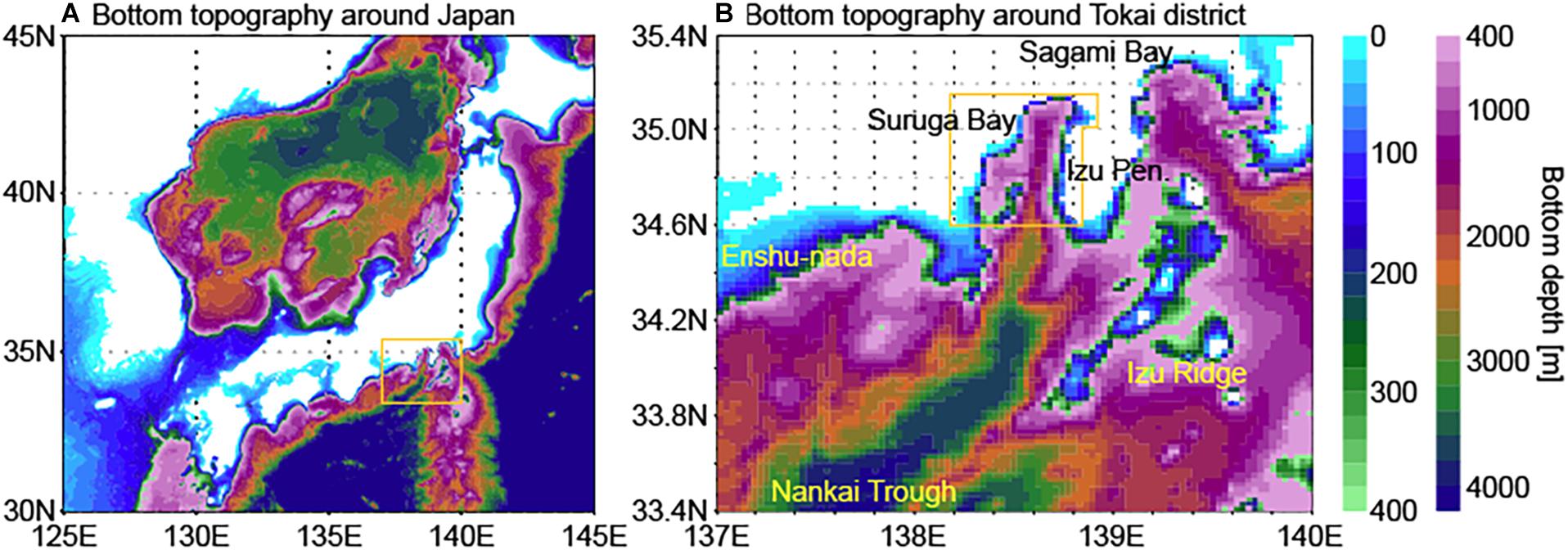
Figure 1. Bottom topography of the ocean reanalysis product around Japan (A) and around the Tokai district (B). Yellow line in (A) indicates the boundary of (B). Yellow line in (B) indicates Suruga Bay as defined in this study.

The processes by which the Kuroshio water intrudes into the bay are rather complicated. Kimura (1950) showed the existence of a cyclonic circulation over Suruga Bay by means of drifting bottles, which was also implied from bay-wide hydrographic observations (Sato, 1967). Later, an accumulation of hydrographic data enabled the circulation variability to be estimated, with a predominant cyclonic circulation (76%) and an anticyclonic circulation (18%) appearing sporadically (Nakamura and Muranaka, 1979). In addition to hydrographic surveys, current measurements have also been conducted (e.g., Inaba, 1982, 1984; Katsumata, 2004, 2016). Besides the predominant semi-diurnal and diurnal tidal currents (e.g., Inaba, 1981; Takeuchi and Hibiya, 1997), both northward and southward surface-layer currents were observed on a longer time scale (more than a day) at stations on the western and eastern sides of the bay mouth. These observations further indicated that the northward (southward) current in the eastern bay mouth and the southward (northward) current in the western bay mouth tend to appear simultaneously when the location of the Kuroshio axis fluctuates to the north (south) (Inaba, 1984). Based on these observations, a schematic picture was drawn for the surface-layer current in the southern part of Suruga Bay that cyclonic and anti-cyclonic circulations appear intermittently, affected by Kuroshio water intrusions (Inaba et al., 2001). These variations can extend vertically downward to at least 200–300 m depth (Inaba et al., 2001; Katsumata, 2016).

Awaji et al. (1991) found that, besides a long-term variation associated with transitions of the Kuroshio path south of Japan (Kawabe, 1986), notable short-term variations in the Kuroshio axis with a period of about 1 month and an amplitude exceeding a few tens of kilometers occur regardless of the Kuroshio path. In addition, their numerical experiments revealed that, in the shelf and coastal region south of Japan, the formation and disappearance of eddies repeatedly take place in response to the short-term transitions in the Kuroshio axis, leading to drastic changes in the coastal currents and water exchange between the coastal region and the Kuroshio. A time scale of 30 days for the Kuroshio fluctuations was also indicated by using HF radar observations to the south of Sagami Bay (Ramp et al., 2008). Miyama and Miyazawa (2014), by using a high-resolution ocean model, detected predominant frontal-wave fluctuations on a time scale of 18–36 days along the Kuroshio and zonally from Shiono-misaki to the Izu Ridge. They further indicated that the amplitude of the fluctuations is relatively large when the Kuroshio takes a nearshore path. In Suruga Bay, typical time scales for the surface-layer current variations were estimated from spectrum analyses of the above-described current observations as 37 and 18 days by Inaba et al. (2001) and as 20–25 days by Katsumata (2016). Katsumata (2016) also estimated the period of the Kuroshio axis fluctuations, which generated the warm-water intrusion events to Suruga Bay, as 25.6 days by using high-frequency tide-gauge data. These previous studies suggested that the Kuroshio fluctuations on a time scale of about 1 month play an important role in generating the coastal current variations in and around Suruga Bay.

Recently, Sugimoto et al. (2020) showed that, when the Kuroshio takes a large meander (LM) path (Figure 2A), marked coastal warming from the surface down to as much as 300 m appears off the Tokai distinct despite the existence of a cool water pool within the large meandering between the Kuroshio and the southern coast of Japan. They clarified that the coastal warming is attributed to the westward Kuroshio bifurcation at around 138°E, 34°N. Note that Suruga Bay was included in this warming region of their analysis. Thus, the long-term Kuroshio path variations also affect the coastal region around Suruga Bay. Katsumata (2016) discussed that the Kuroshio path being close to Suruga Bay (within 120 km) is a necessary condition for the short-term Kuroshio fluctuations to affect the bay. However, the above-described current observations in Suruga Bay investigated the Kuroshio water intrusions during the periods 1977–1980 (Inaba, 1984) and 1990 (Katsumata, 2016), when the Kuroshio took the LM path; during the period 1997–1999, which was investigated by Inaba et al. (2001), the Kuroshio took a relatively small but obvious meander path (offshore non-LM (oNLM) path; e.g., Kawabe, 2005). Thus, the varying influence of the Kuroshio water depending on the Kuroshio path types has not been clarified sufficiently. In addition, the time evolution of the generation of circulation patterns should be further examined.

FIGURE 2

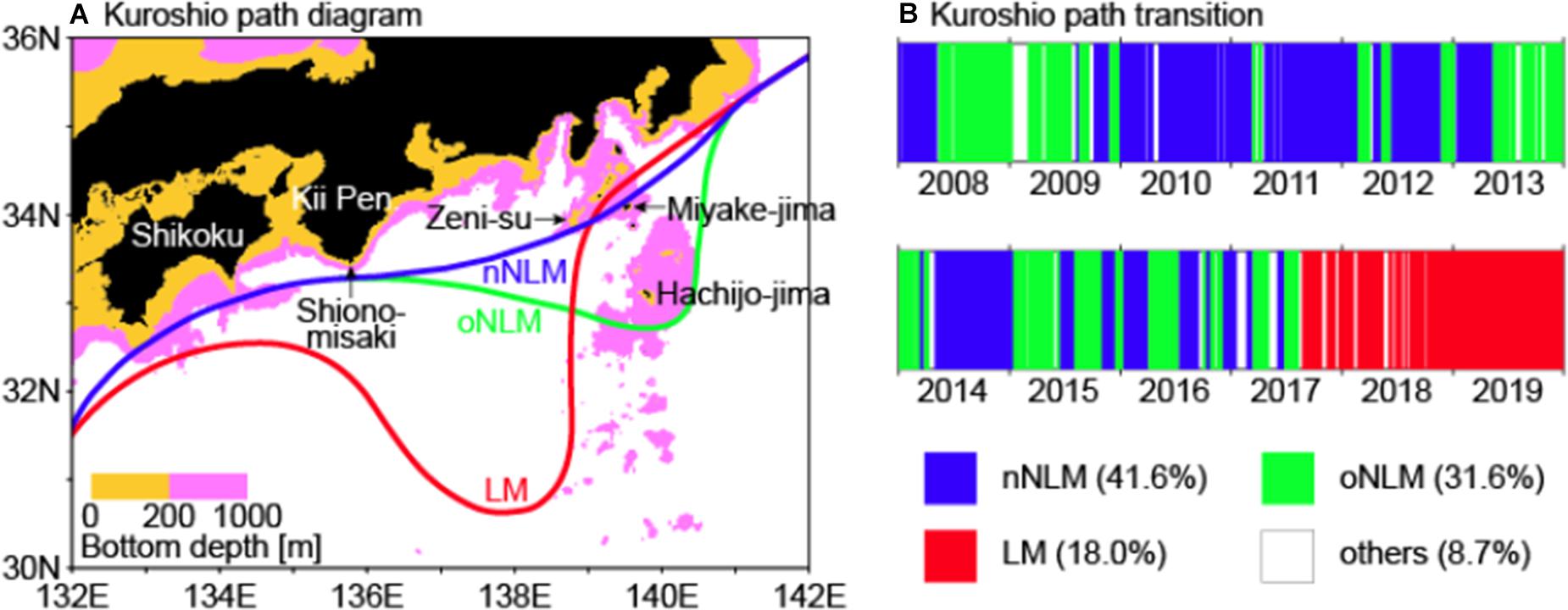
Figure 2. (A) Three typical paths of the Kuroshio: nearshore non-large meander (nNLM), offshore non-large meander (oNLM), and large meander (LM). These path lines were traced from Kawabe (1995). (B) Transition of the Kuroshio path during the period 2008–2019 as defined by using the simulation product.

In this study, we investigated the spatial structure and driving process of the surface-layer circulation variability associated with the Kuroshio water intrusions, which have not been fully clarified because of the limitations of observational data. For this purpose, we used a high-resolution ocean data-assimilative simulation product (Hirose et al., 2019). This product was derived by using a sophisticated system, with an explicit representation of the main tidal constituents and a four-dimensional variational data assimilation technique, for example. Taking into consideration the difference between the typical horizontal scale of the Kuroshio meandering and the bifurcation flow (a few hundreds of km) and the width of Suruga Bay (about 50 km), frontal waves (Miyama and Miyazawa, 2014) around the large-scale Kuroshio structures would be the direct contributors to the inflow to the bay. Hence, processes on a scale that is smaller than meso-scale eddies (e.g., 15 km for the width of the intrusions; Katsumata, 2004) would be necessary to represent the intrusion events. A nesting approach adopted in the simulation system enabled the product to represent the Kuroshio and coastal regions around Japan with a horizontal resolution of about 2 km. Thus, a detailed analysis including the variability within the bay is possible under a realistic reproduction of the larger-scale background conditions (e.g., locations of the Kuroshio axis and meso-scale eddies) by data assimilation. Relationship between the flow to the south of Suruga Bay and the generation of circulation patterns in the bay (as depicted from limited observations in previous studies) is quantitatively investigated for individual three typical Kuroshio path periods which are covered by the simulation product (2008–2019). By using this product, we examined the dynamic structure of the surface circulation of Suruga Bay. The results were validated by available observations. These analyses of the processes for generating surface-layer circulation variability provide useful information for understanding the regional climate and ecosystem in Suruga Bay.

The simulation product and other data used for validating its reproduction are described in section “Materials and Methods.” The variability in the surface-layer circulation in Suruga Bay is investigated by using the simulation product and the processes that generate the circulation patterns are discussed in section “Results.” A summary and further discussion are provided in section “Summary and Discussion.”

Materials and Methods

We use an ocean data-assimilative simulation product for the period 2008–2019 derived from the MOVE/MRI.COM-JPN system (Hirose et al., 2019). This system was based on an ocean general circulation model developed by the Meteorological Research Institute (MRI), MRI.COM version 4 (Tsujino et al., 2017). The surface boundary conditions were given by the 3-hourly JRA55-do dataset (Tsujino et al., 2018). Three domains (global, North Pacific, and around Japan) were connected through a nesting technique; the innermost domain around Japan (117–160°E, 20–52°N) has a resolution of 1/33° zonally and 1/50° meridionally (about 2 km). Various satellite and in situ observations were assimilated in the outer two domains and the assimilation increments obtained there were also used in the inner domain (around Japan) to constrain the meso-scale variations. Note that sea surface temperature (SST) data were not assimilated in several coastal areas including Suruga Bay based on the data resolution of 1/4° (MGDSST; Kurihara et al., 2006). Details of this sophisticated system were described by Hirose et al. (2019). See also Usui et al. (2017) for details of the data assimilation method and the assimilated data.

Validation of the simulation product (for their study period 2008–2017) was provided by Hirose et al. (2019). In addition to the constraint to observation data of large-scale SST and sea surface height (SSH) fields, power spectra of in situ SSTs (buoy observations) at station Mera and Uchiura (in southeastern and northeastern Suruga Bay) were realistically reproduced by the simulation product, in contrast to the MGDSST particularly in the high-frequency domain (shorter period than a few month); comparison of SSHs with tide-gauge data showed correlation coefficients (capture ratios) of 0.91–0.93 (0.83–0.88) at 6 stations around Suruga Bay, 0.95 (0.90) and 0.98 (0.96) at Miyake-jima and Hachijo-jima, respectively.

In this study, daily climatologies were calculated on each grid by averaging over the product period 2008–2019 and were used to remove the mean seasonal variation. In addition, the types of Kuroshio path were defined by using daily horizontal velocities at 100 m depth of the simulation product. Conditions for the LM path were set as follows (e.g., Miyama et al., 2018): (1) the Kuroshio axis (horizontal velocity maximum at 135.5–136°E) separates from Shiono-misaki (south of 33°N); (2) the southernmost location of the Kuroshio axis (averaged over 0.5° bins between 136 and 138°E) is situated south of 32°N; and (3) the Kuroshio axis is located north of Hachijo-jima (north of 33.1°N at 139.5–140°E) or west of Hachijo-jima (west of 139.8°E at 32.7–33.2°N). When conditions (1) or (2) were not satisfied, the path type was classified as NLM paths: the nearshore NLM (nNLM) path satisfies condition (3) and the offshore NLM (oNLM) path does not. The remaining paths were classified as “others,” which represents the transitioning paths between the above typical paths. In addition, when a path type did not appear stably (no longer than 10 days), it was also classified as “others.” The durations of these paths (Figure 2B) were mostly consistent with previous studies (e.g., Sugimoto et al., 2020).

A gridded SSH and surface velocity product with 0.25° resolution (Mertz et al., 2018) was provided by the Copernicus Marine and Environment Monitoring Service (CMEMS). SST estimates with 2 km resolution based on measurements from the Himawari-8 geostationary satellite (Kurihara et al., 2016) were provided by the Japan Aerospace Exploration Agency. Sea level observations at tide gauge stations around Japan were provided by the Japan Oceanographic Data Center. We use time series of the observation data at tide-gauge stations, Tago and Yaizu. The data at these stations were collected by the Geospatial Information Authority of Japan.

Current data based on acoustic Doppler current profiler (ADCP; Teledyne RD Instruments Workhorse Sentinel 300 kHz) observations from the sightseeing ferry Fuji, round-tripping between Shimizu Harbor and Toi Harbor four times a day (Niki et al., 2014), were used. The original data include predominant diurnal and semi-diurnal tidal current variations (e.g., Inaba, 1981), which are not targets of this study. In order to eliminate tidal components from these snapshot data (during the daytime operations only), we carried out the following process. (1) The ADCP data were sorted onto the model grid bins horizontally. Vertically, grids with intervals of 4 m were set as the ADCP observations. Hourly averages were calculated on each grid. (2) Hourly climatology time series were calculated for these gridded hourly data by averaging interannually (2008–2018; overlapped period between the ferry data and the simulation product), which include from seasonal to intra-daily variabilities. (Climatology was not defined for hours when the ferry did not operate, such as at night). (3) Hourly anomaly time series were calculated from these differences. (4) Daily mean anomaly time series were derived from available hourly anomaly data.

Results

EOF Mode Decomposition

First, we examined the horizontal velocity field at a surface-layer depth in the simulation product. We used values at the sixth level grid whose vertical spacing, 18–26 m, includes 20 m depth as investigated from direct measurements by using current meters in previous studies (e.g., Inaba, 1984; Inaba et al., 2001; Katsumata, 2016). In this study, Suruga Bay was defined as the region to the north of the 34.6°N zonal line (within the region bounded by the yellow line in Figure 1B; e.g., Tanaka et al., 2008).

As a long-term mean for the simulation product field (2008–2019), an anti-cyclonic circulation over the central and southern parts of Suruga Bay was obtained (Figure 3A). Maximum speed, smaller than 10 cm s^–1, was seen near the eastern bay mouth. For the variational components of zonal and meridional velocities, we performed a combined empirical orthogonal function (EOF) analysis. The daily mean time series of the horizontal velocities (zonal and meridional components) at 20 m depth in Suruga Bay during our study period of 2008–2019 were decomposed into the EOF modes. Note that mean seasonal cycle was not removed for this analysis, the validity of which is discussed later in association with comparison of monthly occurrences of the EOF modes (Figure 4C). Obtained first to third leading EOF modes (hereafter, EOF1, EOF2, and EOF3, respectively) explained 41, 16, and 9% of the total variance. Higher modes exhibited variations on much smaller scales and explained less than 5% of the total variance (not discussed in this study). The EOF1 pattern showed a circulation similar to the previous schematic picture (Inaba, 1988; Inaba et al., 2001), e.g., when the EOF1 time coefficient is positive, northward inflow in the eastern side of the bay mouth and southward outflow in the western side are connected by a half-round cyclonic circulation in the central–southern part of the bay (Figure 3B). Note that circulation patterns in the bay head region as drawn in the previous schematic picture were not captured in our analysis. The distribution of the meridional velocities on a vertical cross section in the middle of the cyclonic circulation (along the 34.75°N line; red dashed line in Figure 3B) indicated that the circulation pattern at 20 m depth extends to 200–300 m depth (Figure 3F). Here, projections to the EOF time series were plotted for the values outside Suruga Bay and other than at 20 m depth. The EOF2 pattern showed a rather closed circulation in the central part and inflow and outflow at the bay mouth connected in the southernmost part of the bay (Figure 3C). The positive (negative) EOF3 pattern showed basically southward (northward) surface-layer flow in the bay (Figure 3D). Magnitudes of these velocity variations for EOF2 and EOF3 were smaller than that for EOF1 (Figures 3G,H).

FIGURE 3

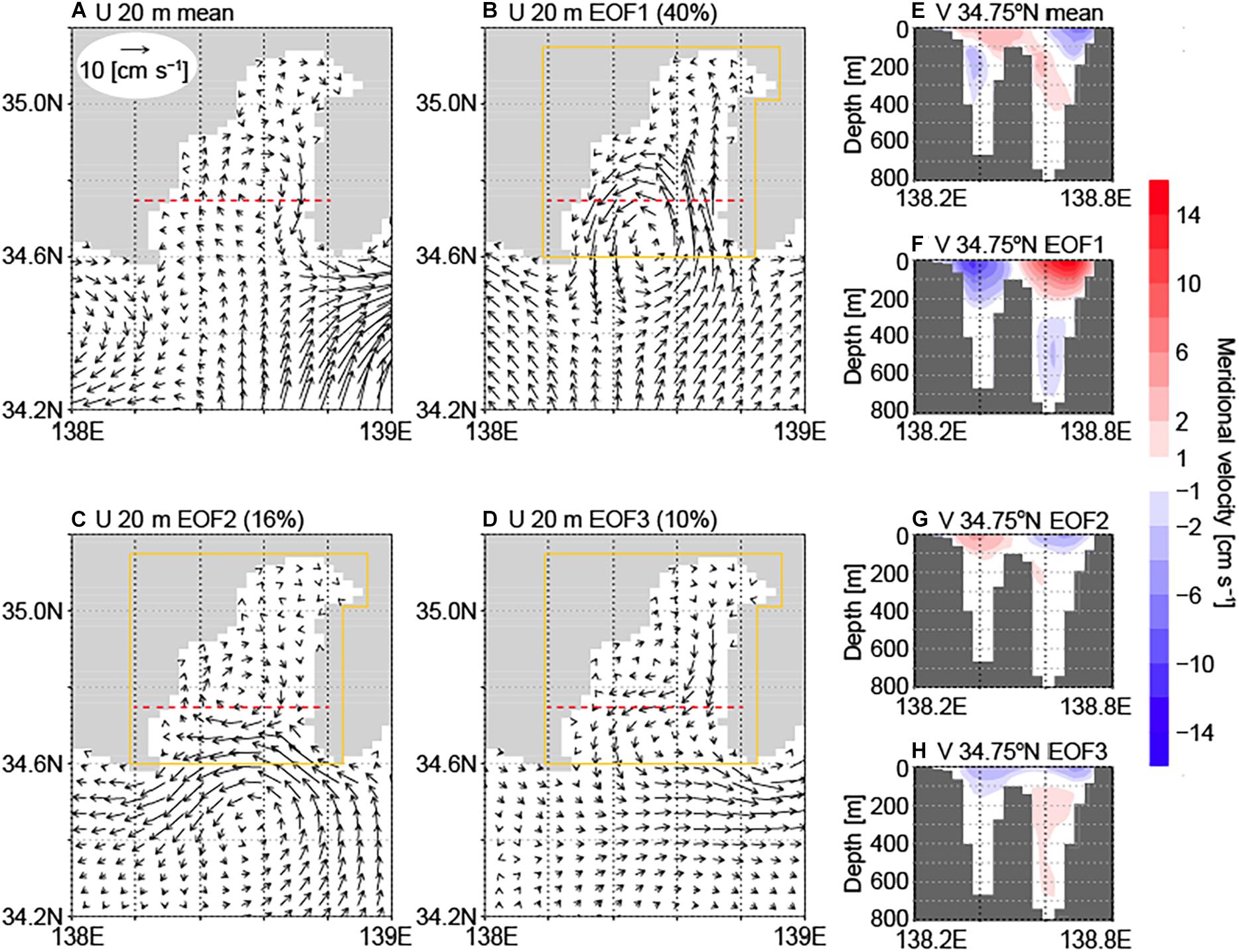
Figure 3. (A–D) Distributions of horizontal velocities at 20 m depth. (E–H) Distributions of the meridional velocities on the vertical cross section along the 34.75°N line as indicated by red dashed lines in (A–D). (A,E) Long-term mean field averaged over the product period 2008–2019. (B,F) EOF1. (C,G) EOF2. (D,H) EOF3. EOF analysis was conducted for the 20 m velocities in Suruga Bay (inside yellow lines) and projections to the EOF time series were plotted in the other region for (B–D,F–H).

FIGURE 4

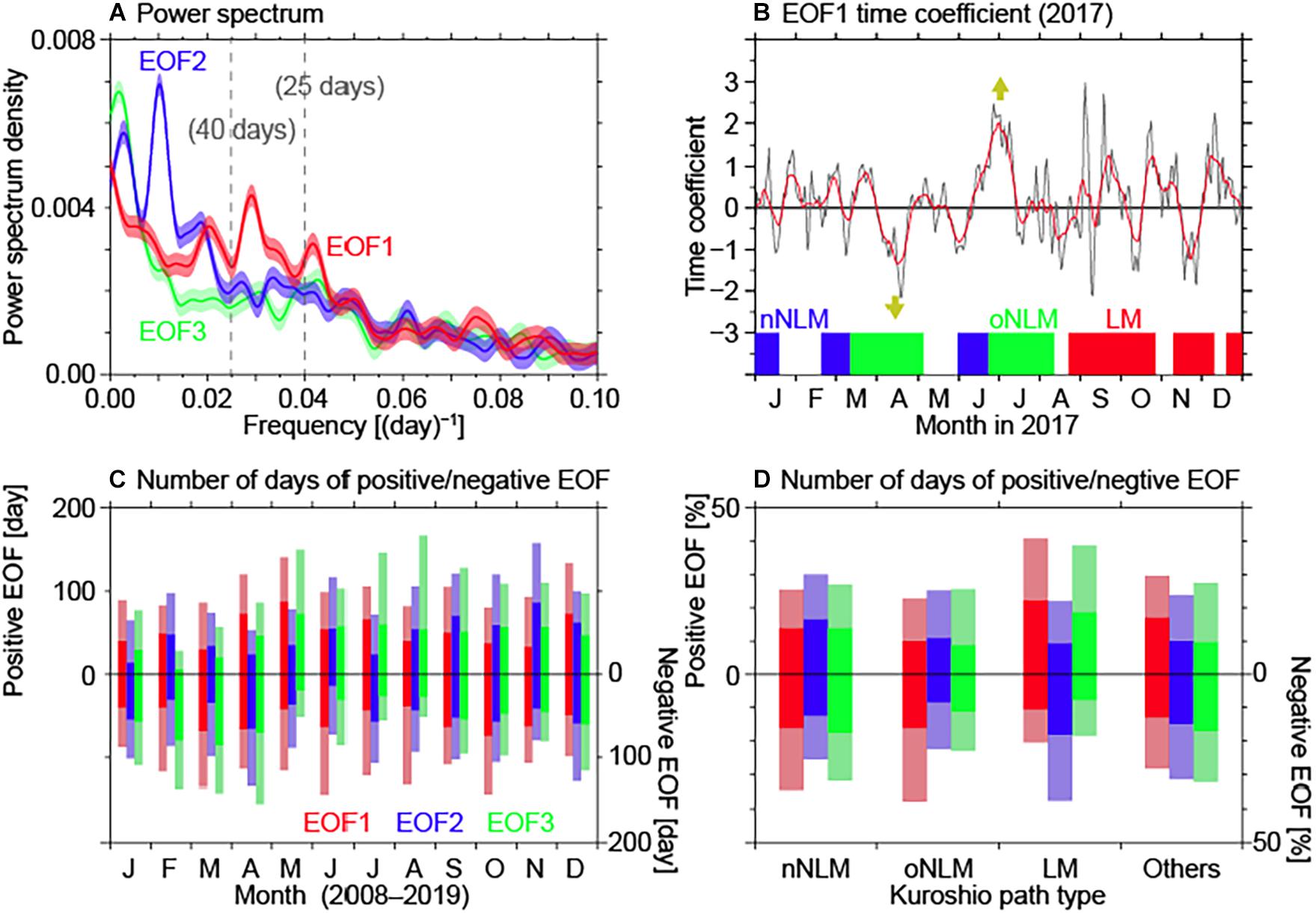
Figure 4. (A) Power spectra for daily time coefficients of the EOF modes (red, blue, and green for EOF1, EOF2, and EOF3, respectively) based on the fast Fourier transform method. A Tukey filter with the effective width of 0.005 [frequency in (day)^{– 1}] was applied. Shading denotes the 1% significance level. (B) Daily and smoothed (11-day running mean) time series of the time coefficients of EOF1 for 2017 (black and red line, respectively). The Kuroshio path types are indicated by color bars as in Figure 2B. (C) Total number of days when the EOF time coefficient (red, blue, and green for EOF1, EOF2, and EOF3, respectively) is greater than +1 (left axis; upper half) and smaller than −1 (right axis; lower half) for each month during the period 2008–2019 (thick colors). Thin colors indicate the same but using a threshold of ±0.5. (D) Same as (C) but for each type of the Kuroshio path and units are in % of the total days for each type.

A spectrum analysis of the time series of the EOF time coefficients (Figure 4A) indicated that the EOF1 mode (red line) takes a peak power spectrum density on a time scale of about 25–40 days [frequencies of 0.04 to 0.025 (day)^–1]; the EOF2 mode takes power spectrum density peaks of around 100 days and 1 year (blue line) and the EOF3 mode takes a peak of around 1 year (green line). Actually, repeated variations on a time scale of about 1 month can be seen in the EOF1 time series for 2017, for example (Figure 4B; see Supplementary Figure 1 for the whole product period 2008–2019). In addition, we counted the number of days when the time coefficient takes a large value (Figures 4C,D; thresholds of 0.5 and 1 (light and thick color bars, respectively) were used for these figures, but the conclusions are not changed by summing the positive/negative EOF values). Mean monthly values for this number during the whole period 2008–2019 did not exhibit a notable seasonal signal for EOF1 (Figure 4C). These features of the EOF1 pattern and time series representing bay-scale and surface-layer (about 0–200 m depth) circulation pattern variation on a time scale of about 1 month were consistent with the cyclonic and anti-cyclonic pattern variation as described in previous observational studies (e.g., Inaba, 1984; Katsumata, 2016). Therefore, we considered that the observed short-term variations in the surface-layer current in Suruga Bay were generally captured by the EOF1 mode. The EOF2 mode with another horizontal circulation pattern and the EOF3 mode with an overturning pattern (Figure 3) might have an additional effect on the circulation variability. Note that, for EOF2 (blue bars in Figure 4C), the number of days with large positive values was notably larger (smaller) than the number with large negative values in August–November (January–May); the number of positive-value days was relatively large in May–August and relatively small in February–March for EOF3 (green bars in Figure 4C). Thus, the mean seasonal variation was reflected in these modes, although the intensities of these modes also varied interannually. For a measure of the interannual variability, numbers of days with large (negative/positive) EOF time coefficients were counted for the individual Kuroshio path periods (Figure 4D). Similar numbers of days were counted for the negative and positive EOF1 days during the nNLM and oNLM periods, although slightly larger numbers of negative EOF1 days than positive EOF1 days were seen with the threshold of 0.5. During the LM path period, the number of days was much larger for positive EOF1 than for negative EOF1 based on both thresholds of 0.5 and 1. This suggested that environmental conditions, such as the type of Kuroshio path, influence the occurrence of the intrusions into Suruga Bay and related generation of the bay-wide circulation patterns. In addition, during the LM path period, the number of days was larger for negative EOF2 than for positive EOF2 and also larger for positive EOF3 than for negative EOF3, as discussed later (see section “Summary and Discussion”).

Large-Scale Environments for Generating Intrusion Circulations

Hereafter, we mainly focus on the processes for generation of the EOF1 circulation pattern (Figure 3B), which would be associated with the open-ocean water intrusions. We investigated the conditions associated with the EOF mode outside Suruga Bay. Since the types of Kuroshio path greatly influence the large-scale temperature and velocity distributions, averages/composites of the EOF1 mode over the period including several Kuroshio path types would be mainly determined by fractions of the periods for the path types, and hence inadequate for our purpose. Instead, we took composites of daily potential temperature anomaly and horizontal velocity fields of large EOF1 time coefficient (EOF1 < −1 and EOF1 > +1) for the three typical Kuroshio path periods (Figure 2B) separately. The 100-m depth fields were used for reducing the near-surface variability due to surface forcing. As assumed for this classification, both negative and positive EOF1 composites represented the large-scale characteristics of the Kuroshio path types: the Kuroshio passes relatively near the coast with warm anomalies along the path between 135 and 141°E during the nNLM period (Figures 5A,B); the Kuroshio passes south of Hachijo-jima with cold anomalies between 137 and 141°E to the coastal side during the oNLM period (Figures 5C,D); the Kuroshio separates from the Kii Peninsula (about 136°E), meanders to the south of 32°N around 137–138°E and then northward, and flows along the coast of the Kanto district (about 139–140°E) during the LM period (Figures 5E,F). These gross features were consistent with previous studies (e.g., Kawabe, 2005). Differences between the negative and positive composites were examined for each Kuroshio path period as described below.

FIGURE 5

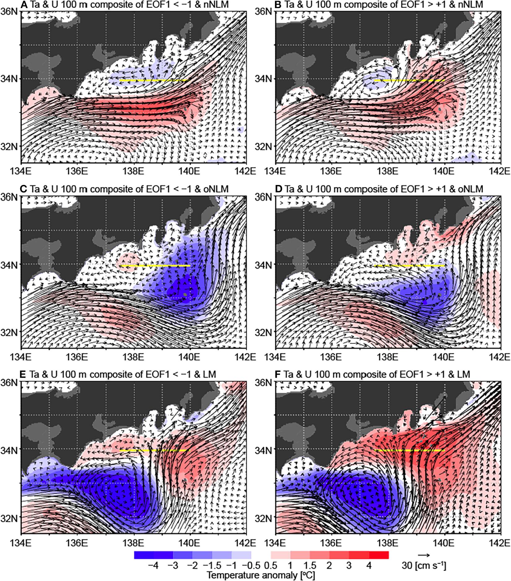
Figure 5. Horizontal distributions of potential temperature anomalies (from daily climatologies; shading) and velocities (arrows) at 100 m depth. Composites of the daily values when the EOF1 time coefficient is smaller than −1 (A,C,E) and greater than +1 (B,D,F) for the nNLM (A,B), oNLM (C,D), and LM (E,F) periods. Yellow lines denote the 33.95°N zonal section as examined in Figure 6.

From a comparison between the negative and positive EOF1 composites during the nNLM period (Figures 5A,B), the negative EOF1 composite exhibited more zonally spread cold anomalies between the Kuroshio and the whole Tokai district, whereas the cold anomalies were relatively confined around Enshu-nada for the positive composite. Northward flow was seen to the east of these cold anomalies and this partly directed to Suruga Bay for the positive composite case. From a comparison during the oNLM period (Figures 5C,D), cold anomalies inside the Kuroshio meandering extended between the Kuroshio and the Kanto district, and the Kuroshio mostly flowed to the east of Hachijo-jima for the negative EOF1 composite; for the positive composite, a branch flow bifurcated around 139°E, 33°N, and partly turned in direction northeastward along the coast from Suruga Bay to the Kanto district, forming warm anomalies. From a comparison during the LM period (Figures 5E,F), the northward Kuroshio flow around 138–140°E extended more widely for the positive composite than for the negative composite, resulting in stronger flow toward Suruga Bay for the former case with warmer anomalies along the Tokai and Kanto districts.

Inaba et al. (2001) indicated that the position of the Kuroshio axis relative to a shallow group reef, Zeni-su, (about 75 km south of the southern cape of Izu Peninsula, Irozaki) can be a useful measure of the influence of the Kuroshio water on Suruga Bay. We examined the composite velocities on the zonal section crossing Zeni-su (33.95°N; yellow lines in Figure 5). During the nNLM path period, the Kuroshio passed mainly to the east of Zeni-su for the negative EOF1 composite (Figure 6A), whereas large northward velocities (40 cm s^–1) in the surface layer were seen for the positive EOF1 composite (Figure 6B). Note that relatively large velocities were also seen around 139.5 and 139.9°E, to the west of shallow regions related to Mikura-jima and Izu Ridge, respectively. During the oNLM path period, although the Kuroshio mainly flowed to the east of this cross section (Figures 5C,D), relatively large northward velocities (>15 cm s^–1) associated with the above-described branch flow were also seen to the west of Zeni-su for the positive EOF1 composite (Figure 6D) in contrast to the negative EOF1 composite (Figure 6C). During the LM path period, large northward velocities (>50 cm s^–1) were centered to the east of Zeni-su for the negative EOF1 composite (Figure 6E); large northward velocities (>30 cm s^–1) were seen on both sides of Zeni-su for the positive EOF1 composite (Figure 6F), although these were small in magnitude relative to the peak value for the negative composite and to the subsurface northward velocities associated with the above-described eastern shallow regions. These results (Figures 5, 6) generally supported the relationship deduced from limited observations in previous studies. In addition, our results suggested that the Kuroshio branch flow to the west of Zeni-su, instead of the main axis, is important in cases where the Kuroshio main flow passes far from the region around Zeni-su (i.e., to the east of Izu Ridge) during the oNLM period.

FIGURE 6

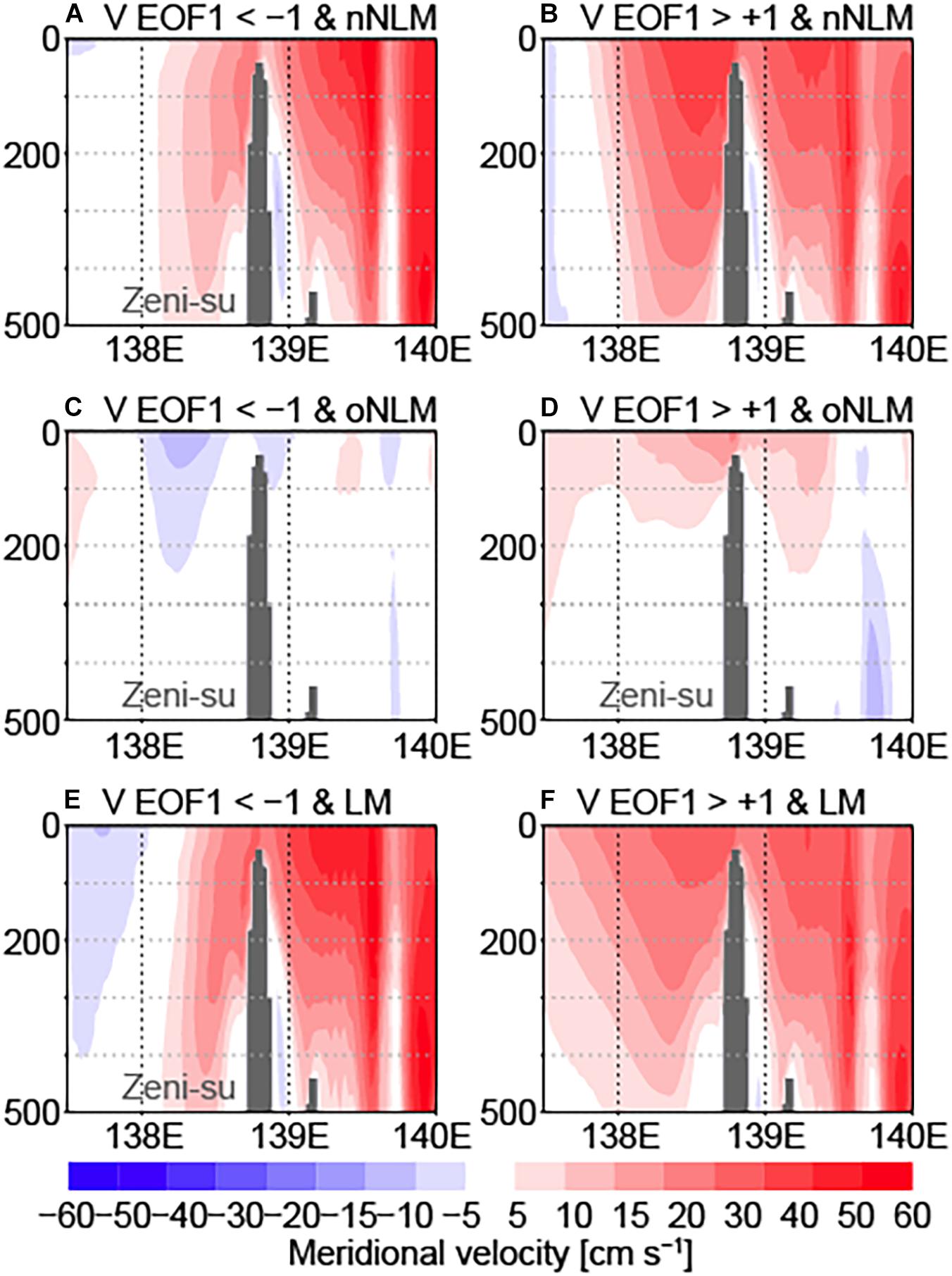
Figure 6. Same as Figure 5 but for meridional velocities on the vertical cross section along 33.95°N (yellow lines in Figure 5).

Examples of Cyclonic and Anti-cyclonic Circulation Events

In order to advance our understanding of the process involved in the Kuroshio water intrusions and generation of the circulation pattern (EOF1), we examine time evolutions of event examples in this section. We selected a negative event in April 2017 (EOF1 time coefficient <-0.5 from 3 to 20 April 2017; downward arrow in Figure 4B) and a positive event in June–July 2017 (EOF1 time coefficient >+0.5 from 11 June to 10 July 2017; upward arrow in Figure 4B). We discuss other events during the whole experimental period later.

Current distributions before the events are shown in Figure 7. On 2 April 2017 (Figures 7A,C,E), the Kuroshio took the oNLM path. The Kuroshio flowed northeastward to the east of Hachijo-jima (141–142°E) and then turned to the west around 34°N and again turned to the east along the coast. On 10 June 2017 (Figures 7B,D,F), the Kuroshio took the nNLM path, flowing to the north of Hachijo-jima. These large-scale current distributions as represented in the simulation product (Figures 7C,D) were consistent with the satellite altimeter product (CMEMS; Figures 7A,B). On the other hand, small-scale structures that form around the Kuroshio main flow were not represented in the satellite product (Figures 7A,B) but only visible in the simulation product (Figures 7C–F). As discussed below, generation of the EOF1 pattern flows in Suruga Bay was affected by the latter small-scale structures that were resolved in the simulation product.

FIGURE 7

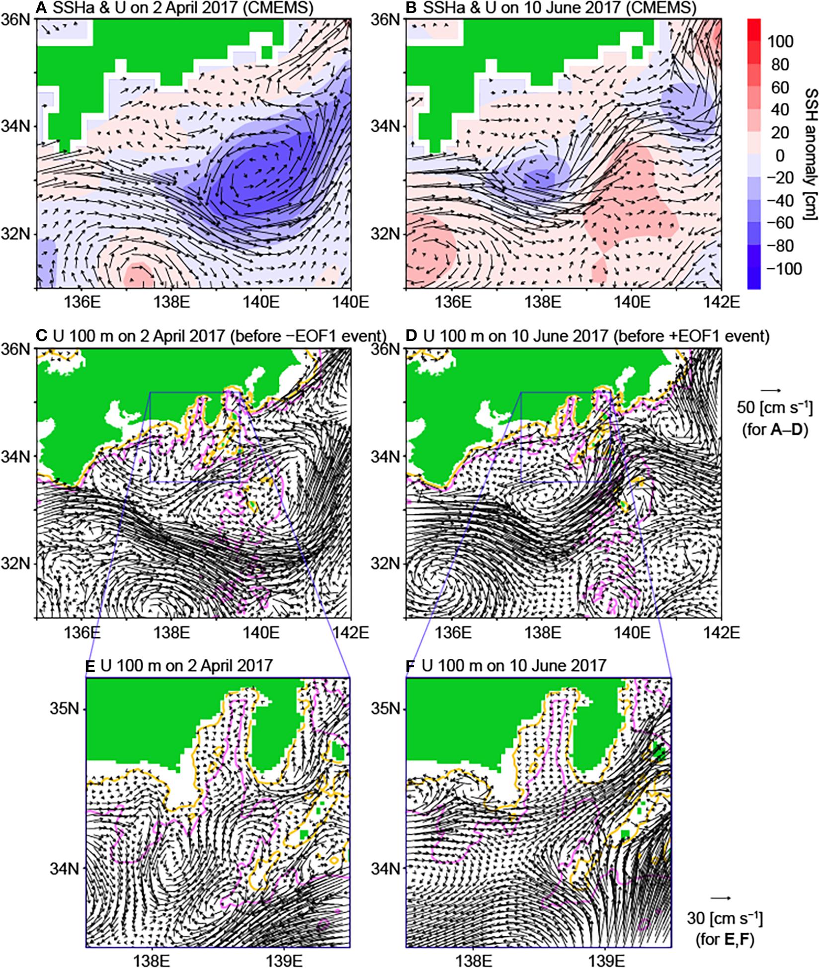
Figure 7. (A,B) Distributions of SSH anomalies and surface velocities from the satellite altimeter product (CMEMS) before the negative (A) and positive (B) EOF1 events (2 April 2017 and 10 June 2017, respectively). (C,D) Distributions of horizontal velocities at 100 m depth on the same days as (A,B) from the simulation product, respectively. Yellow and pink lines indicate 200 and 1,000 m depth isolines (see Figure 2A). (E,F) Same as (C,D) but expanded near Suruga Bay.

We first investigated the development of the positive EOF1 event in detail. On the initial date (10 June 2017), the northward flow to the west of Zeni-su merged with the eastward flow from Enshu-nada, forming a strong eastward flow to the south of the mouth of Suruga Bay (Figure 7F). Figure 8 shows the time evolution of SSH and relative vorticity distributions at 100 m depth during the positive EOF1 event. Note that SSH isolines roughly indicate the directions of horizontal velocities. On 10 June 2017 (top left; corresponding to Figure 7F), the SSH isolines that passed to the south of the shallow (<100 m) coastal shelf region near the western bay mouth (about 138.2°E, 34.4°N) extended eastward without touching the eastern bay mouth region. Hence, no intrusion occurred from the eastward flow outside the bay. The EOF1 time coefficient was small (0.03) at that time. On day 3 (from the initial day 10 June, i.e., 13 June; “Day+3” in Figure 8), the eastward flow partly went into the eastern part of the bay. Positive vorticities were seen in the intrusion region, which stemmed from the south of the western shallow region. This suggested that the northward intruding fluctuation of the flow can be attributed to the shear-induced positive vorticity inputs in this region (e.g., vorticity supply from the southern tip of Kyushu; Akitomo et al., 1991). The intrusion once ceased on day 6, then took place again on days 9–12, and eventually generated a cyclonic circulation in the central and southern parts of the bay on days 15–18, when the EOF1 time coefficient was greater than 2. On day 18, the strong circulation shifted southward, suppressing the northward fluctuation of the eastward flow to the south. Without additional intrusion, the circulation in the bay weakened on day 21 and then merged into the eastward flow outside the bay on day 24. Although the EOF1 time coefficient was still large on day 27, the cyclonic circulation was migrating out of the bay. The event terminated when the circulation was fully discharged.

FIGURE 8

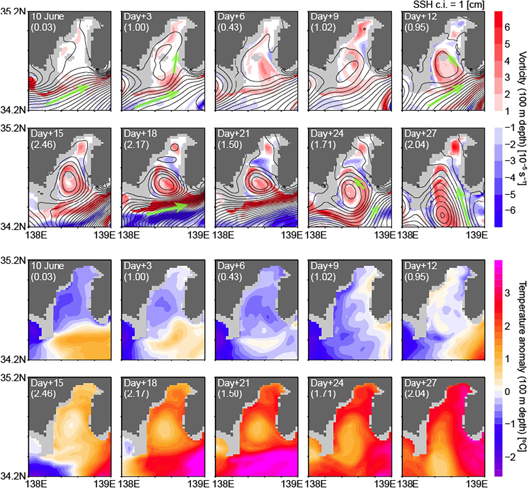
Figure 8. Distributions of SSHs (contours with 1 cm intervals) and relative vorticities at 100 m depth (shading) (upper 2 rows) and potential temperature anomalies at 100 m depth (lower 2 rows) during a positive EOF1 event starting from 10 June 2017 (top left). Time series for every 3 days are plotted (top left to top right and then bottom left to bottom right for each series). Days from 10 June and the EOF1 time coefficient are indicated in each figure. Relative vorticity was defined in this study as ζ = v_x−u_y, where u and v are zonal (x-ward) and meridional (y-ward) components of horizontal velocity, respectively. Broad flow directions are indicated by green arrows.

The time evolution of potential temperature anomalies (from daily climatologies) at 100 m depth during the event is also shown in Figure 8. In the beginning (10 June), there existed cold anomalies both inside the bay and in the region extending southward from the bay mouth bounded by shallows on both the western and eastern sides (light gray for regions <100 m depth in Figure 8) and warm anomalies to the south. The eastward flow (Figure 7F) prevailed in the transition region between the cold and warm anomalies. When the intrusion event began (day 3), the circulation pattern was reflected in the potential temperature field; cold anomalies were concentrated near the center of the circulation. On day 9, the positive vorticities associated with the intrusion extended to almost the northern bay head, where the intrusion flow turned anti-clockwise to the south; at that time, cold anomalies weakened in the east of the bay (Figure 8). Afterward, the region to the south of the bay gradually became warmer. As a result, the region outside the bay was mostly occupied by relatively warm water on days 15–18, leading to further increases of the warm anomalies in Suruga Bay through the intrusions, while the contrast in the potential temperatures between the center and rim of the circulation remained. Thus, a large-scale environmental change took place during this intrusion event. This was attributable to an approach of the Kuroshio branch and was also consistent with both warm anomalies to the south of Suruga Bay and relatively strong northward flow to the west of Zeni-su in the composite distributions (Figures 5, 6).

A similar time evolution (on both the large scale and the scale within the bay) was generally seen for the potential temperature anomalies near the surface (e.g., Figure 9C), which suggests that these changes occurred consistently within the surface layer, although surface forcing also has an effect near the surface. Hence, satellite-derived SST data can be used for evaluating our results. Figure 9 compares the SST distributions between the observational estimate and the simulation product on 29 June 2017. Note that the day with less cloud cover and near the EOF1 peak was selected. Relatively warm SSTs in the rim of the central–southern part of Suruga Bay and relatively cold SSTs inside were represented in the simulation product (Figure 9B), which corresponded to northward flow in the eastern part and southward flow in the western part and the doming structure of potential temperature between these flows (e.g., 15 and 20°C (green) isolines in Figure 9C). The above SST distribution was basically captured by the satellite observational estimates (Figure 9A), although the frontal area with large SST gradients was represented relatively in the north in the simulation product.

FIGURE 9

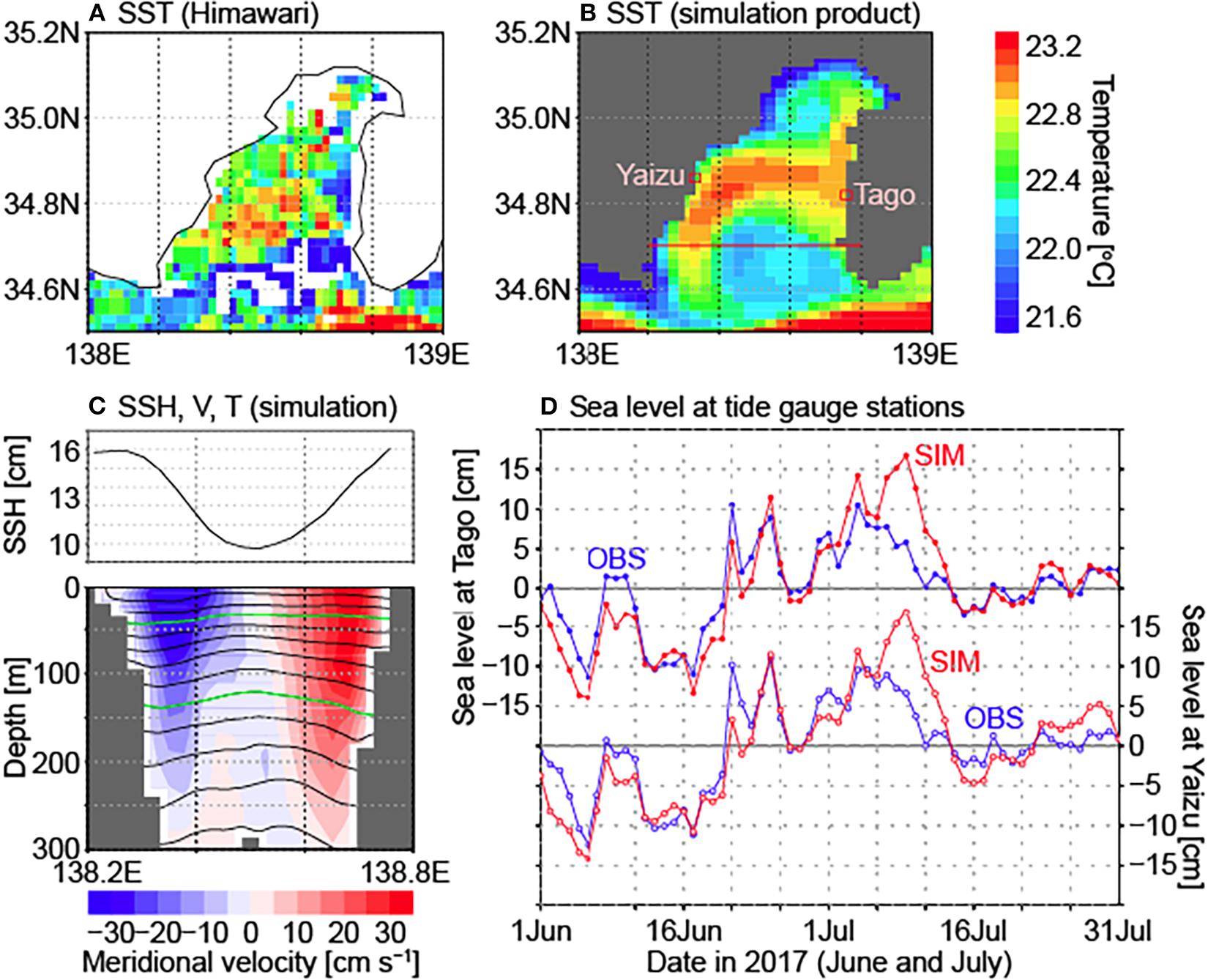
Figure 9. (A) Distribution of SSTs derived from satellite (Himawari-8) observations on 29 June 2017. Missing values are due to cloud cover flags. (B) Same as (A) but from the simulation product. (C) Distributions of SSHs (upper panel), meridional velocities (shading in lower panel), and potential temperature (contours in lower panel with 1°C intervals; green contours indicate 15 and 20°C) along the 34.7°N zonal line [red line in (B)]. (D) Daily time series of sea levels at the tide-gauge stations [red rectangles in (B)], Tago (138.76°E, 34.81°N; closed circles; left axis) and Yaizu (138.33°E, 34.87°N; open circles; right axis), in June and July 2017. Blue and red lines indicate tide-gauge observation data and the simulation product, respectively. Note that these time series include the effect of surface pressure.

In addition, we used the tide-gauge data for another validation of our results, since the above changes in the surface layer were reflected in the SSH field (e.g., Figure 9C). We compared the SSH time series in the simulation product with the sea-level observations at Tago and Yaizu tide-gauge stations (Figure 9D). At both stations, the sea-level increases of about 20 cm from the middle of June to the beginning of July and the decreases afterward were consistently represented in the observational and simulation data; on the other hand, relatively strong and delayed peak was seen on 9 July in the simulation product. Note that comparisons at the other stations in Suruga Bay indicated similar results (not shown). The latter discrepancy can be attributed to the fact that the simulated bay-scale eddy related to the cyclonic circulation pattern in this event extended to the north (about 34.9°N; Figure 9B) compared with the satellite observational estimates (around 34.85°N; Figure 9A), as described for the SST comparison on 29 June. This would affect the following evolution of this eddy, leading to the delayed southward migration in the simulation product. Note that small-scale variations as described for this event were not constraint by the data assimilation (Hirose et al., 2019). Although validation of our results on this scale was not sufficient due to the limitation of observation data, the above validations with the available data supported that this event was basically represented in the simulation product.

As described above, our results showed an increase of the potential temperature anomalies in Suruga Bay during the positive EOF1 event example in June 2017 (Figure 8). It was also considered that the warming through the intrusions can be more effective when the region to the south of Suruga Bay becomes warmer due to the approach of the Kuroshio branch. We next examined whether or not warming similar to this case occurs in the other positive EOF1 events. Figure 10B shows the changes in the potential temperature anomaly during the individual positive EOF1 events as sorted on the basis of the EOF1 peak days. Although the individual time series (thin black lines) fluctuated greatly, an increase of about 0.7°C was seen on average (red line) around the EOF1 peak. After the increase, the temperature gradually decreased to the value before the event on average (about −0.4°C) as the impact of the intrusion events was gradually damped. As shown in Figure 10B (green line), the potential temperature increase was relatively large during the event in June 2017. The magnitude of the temperature change varied greatly among the events: for example, the mean and standard deviation of the temperature change from 2 days before the peak to 1 day after the peak were 0.58 and 0.59°C, respectively. Note that generation of the intrusion flow would depend on large-scale environmental conditions. It was thus suggested that, in the positive EOF1 events, the current variability outside the bay induces the warm water intrusions into Suruga Bay which have a warming effect of about 0.7°C on average, but the thermal conditions outside the bay also vary during the events, resulting in the additional warming/cooling in Suruga Bay with a similar magnitude.

FIGURE 10

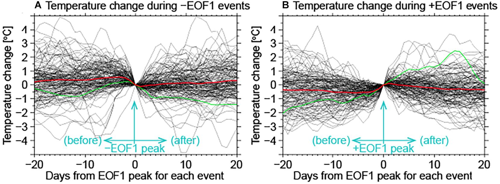
Figure 10. Time series of changes in the potential temperature at 100 m depth in Suruga Bay during the negative (A) and positive (B) EOF1 events. x-axis denotes days from the EOF1 peak; y-axis denotes potential temperature changes from the value on the EOF1 peak day. Thin black lines indicate the individual events. Red line indicates the averaged time series. Green lines in (A,B) indicate the negative EOF1 event in April 2017 and the positive EOF1 event in June 2017, respectively.

We next examined the negative EOF1 mode. At the beginning of the negative EOF1 event in April 2017, a Kuroshio branch flowed southwestward between Zeni-su and Hachijo-jima (Figures 7C,E). Part of this flow circulated clockwise around Enshu-nada, changed direction toward the north to the south of Omaezaki (around 138°E, 33.5°N–34°N) and then passed near Irozaki (eastern cape of the mouth of Suruga Bay) toward Sagami Bay (Figure 7E).

As shown in the time evolution of the SSH and vorticity distributions (Figure 11), a fluctuation upon the above-described large-scale flow to the south of the bay mouth (on 2 April) grew into an anti-cyclonic circulation in the central–southern part of Suruga Bay as seen on days 10–13. In the initial days, this fluctuation took place outside of the meandering of the large-scale flow and was attributable to the inertia effect of this flow (e.g., Usui et al., 2013). A pair of separated cyclonic and anti-cyclonic circulations developed from the fluctuation on day 7. As the large-scale flow migrated southward, the anti-cyclonic (negative vorticity) circulation remained and occupied the central to southern mouth regions of Suruga Bay (days 13 and 16). The EOF1 time coefficient took the largest negative value for this event of −2.17 on day 14 (16 April 2017). As the large-scale flow separated from Irozaki, the anti-cyclonic circulation gradually dissipated without additional inertial vorticity input.

FIGURE 11

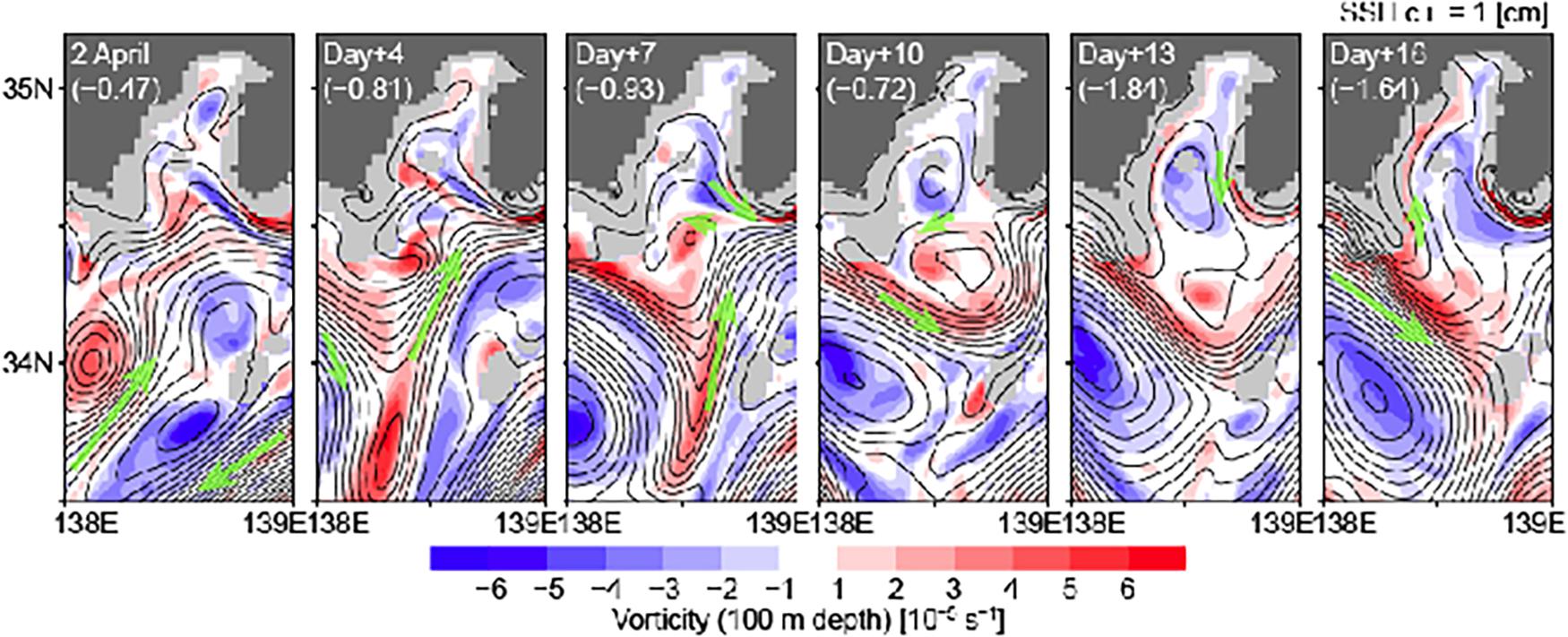
Figure 11. Distributions of SSHs (contours with 1 cm intervals) and relative vorticities at 100 m depth (shading) during a negative EOF1 event starting from 2 April 2017 (left to right). Days from 2 April and the EOF1 time coefficient are indicated in each figure. Broad flow directions are indicated by green arrows.

As described above, the large-scale Kuroshio branch flow migrated southward, away from the bay mouth region, during this event. This generated the temperature decreases around the coastal region, and also in Suruga Bay through the intrusions. Figure 10A shows the potential temperature changes for all negative EOF1 events (including the above example; green line). For the negative EOF1 events, the mean and standard deviation of the temperature changes from 2 days before the peak to 1 day after the peak were estimated as −0.62 and 0.57°C, respectively. The standard deviation value was similar to that for the positive EOF1 events. We discuss below (see section “Relationship Between Flows Over Surrounding Regions”) why the intrusion water is relatively warm in the positive EOF1 events and relatively cold in the negative EOF1 events on average.

The examples of the EOF1 events as presented in this section suggests strong influences of bay-size eddies on the circulation patterns for both negative and positive EOF1 modes. Here, general importance of the bay-size eddies is discussed by examining the composites fields of the negative and positive EOF1 events. As shown in Figure 12, SSH, relative vorticity, and potential temperature anomaly fields of the negative EOF1 composite indicated consistent structures of a bay-scale anti-cyclonic eddy centered near the bay mouth; those of the positive EOF1 composite indicated a bay-scale cyclonic eddy, as seen in the event examples (Figures 8, 11). The circulation pattern of the EOF1 mode (Figures 3B,F) was consistent with the influences of these eddies, including its vertical structure (not shown for the composite fields). These features also corresponded to the co-occurrence of currents with the opposite (northward/southward) directions in the eastern and western bay mouths as indicated by the direct observations (Inaba, 1984). Thus, we concluded that bay-scale anti-cyclonic and cyclonic eddies generally characterize the circulation patterns of the negative and positive EOF1 events, respectively.

FIGURE 12

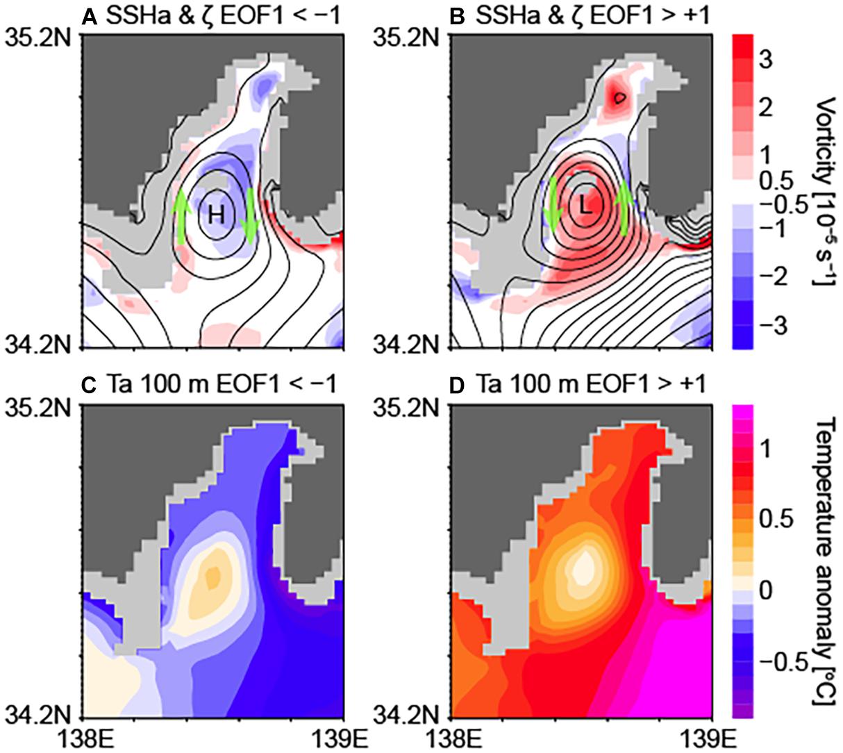
Figure 12. (A,B) Distributions of SSH anomalies (contours with 1 cm intervals) and relative vorticities at 100 m depth (shading). (C,D) Distributions of potential temperature anomalies at 100 m depth. Composites of the daily values when the EOF1 time coefficient is smaller than −1 (A,C) and greater than +1 (B,D). Maximum and minimum locations of the SSH anomaly fields are indicated by “H” and “L,” respectively. Broad flow directions are indicated by green arrows.

Relationship Between Flows Over Surrounding Regions

As described above, the composites and event examples for the positive and negative EOF1 modes represented relatively stronger northward velocities to the west of Zeni-su during the positive EOF1 mode (Figures 5–7), which was basically consistent with the suggestions in previous studies that used the position of the Kuroshio axis. Here, we examine this relationship by using a long-term simulation product. As a measure of the northward flow strength to the west of Zeni-su, we took averages of the meridional velocities at 100 m depth over a section where differences between the negative–positive composite meridional velocities (Figure 6) were relatively large. Note that different sections were assumed for the individual Kuroshio path periods (see caption of Figure 13).

FIGURE 13

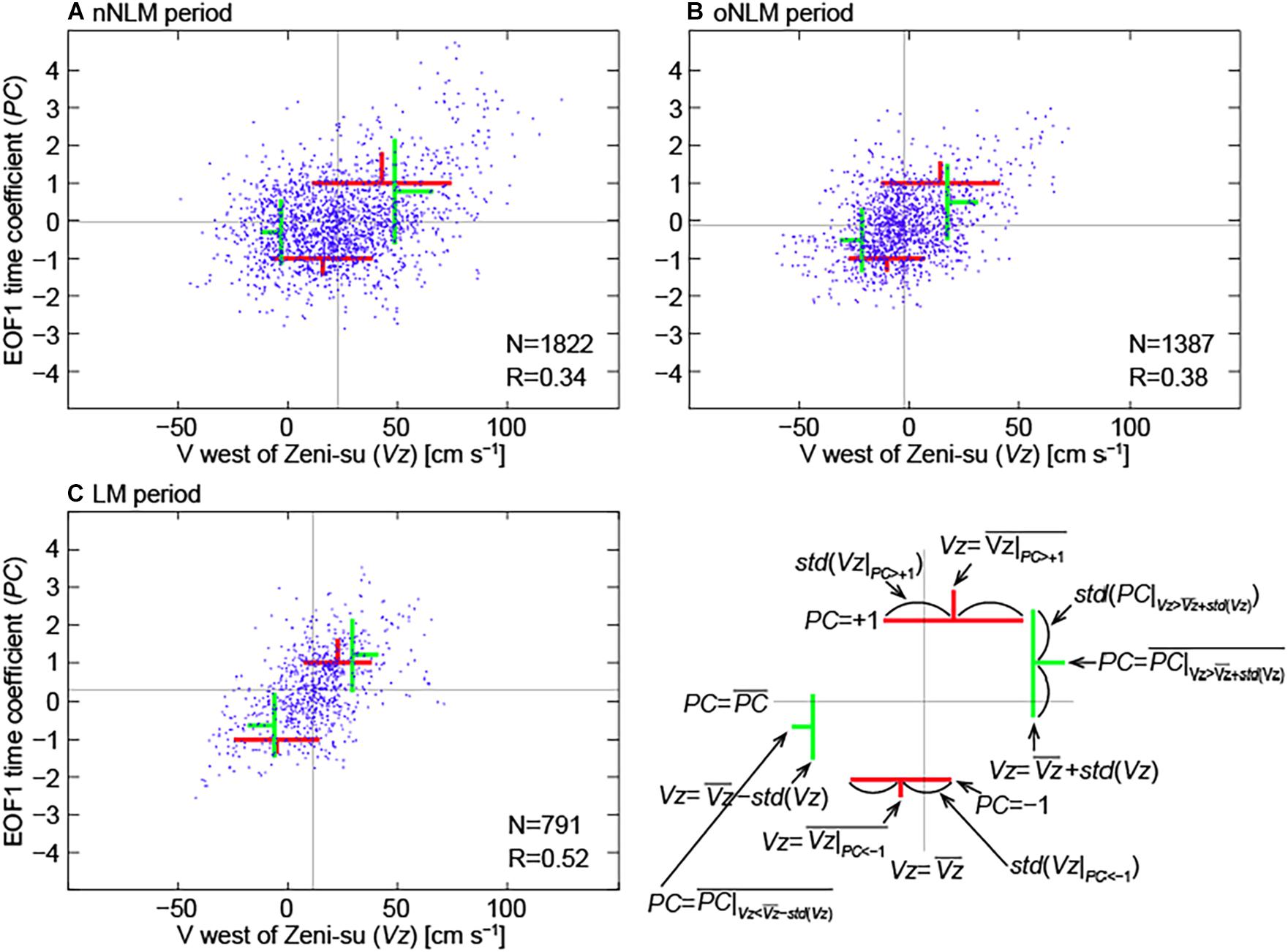
Figure 13. Scatter diagrams between meridional velocity to the west of Zeni-su (Vz) and EOF1 time coefficient (PC) during the individual Kuroshio path period. (A) nNLM. (B) oNLM. (C) LM. Meridional velocities to the west of Zeni-su at 100 m depth were averaged along the 33.95°N line over 138.3°E–138.6°E (A), 138.15°E–138.45°E (B), 137.75°E–138.15°E (C) based on the differences of the positive and negative composites during the individual periods (Figure 6). Lags of PC from Vz by 1, 4, and 3 days for (A–C), respectively, were considered to represent maximum correlations (R). Averages (denoted by overbar) and standard deviations (“std”) of Vz values when PC < −1 and PC > +1 are indicated by red segments. Similarly, averages and standard deviations of PC values when $Vz<\overline{Vz}-std\left(Vz\right)$ and when $Vz>\overline{Vz}+std\left(Vz\right)$ are indicated by green segments.

Figure 13 shows the relationship between the northward flow strength (Vz) and the EOF1 time coefficient (PC). For the individual Kuroshio path periods, positive correlations were detected between Vz and PC. These correlations were significant at 90, 90, and 99% confidence levels for the nNLM, oNLM, and LM periods, respectively (here, the event peak number was used as the least sample number for each period, taking into consideration the autocorrelations of the daily values). As seen in Figure 13, the mean Vz values (indicated by vertical thin gray lines) largely differed between the Kuroshio path periods, which supported the necessity of conducting this analysis separately for the individual periods.

For all three periods, Vz averages over the days with PC > +1 (PC < −1) (vertical red segments) were larger (smaller) than the whole Vz averages (i.e., $\overline{{Vz|}_{PC<-1}}<\overline{Vz}<\overline{{Vz|}_{PC>+1}}$); PC averages over the days with Vz larger (smaller) than $\overline{Vz}$ by one standard deviation (horizontal green segments) were positive (negative). Hence, the suggested relationship basically held for all these periods. However, the relationship was rather weak in several quadrants: Vz averages for PC < −1 (red segments in the third quadrant) were close to $\overline{Vz}$ within a half of the standard deviation during the nNLM and oNLM periods; PC averages for $Vz<\overline{Vz}-std(Vz)$ (green segments in the third quadrant) were rather small (close to zero) during the same periods. Thus, it was suggested that these distributions were skewed during the nNLM and oNLM periods. In contrast, the linear relationship was relatively robust during the LM path period.

As discussed above, the warming of about 0.7°C occurred in Suruga Bay during the positive EOF1 events on average. The relatively strong flow to the west of Zeni-su is consistent with warm anomalies according to the approach of the Kuroshio axis to the Tokai district coast during the nNLM and LM periods (Figures 5B,F) and that of the Kuroshio branch during the oNLM period (Figure 5D). Thus, the warming can generally occur around the coastal region of the Tokai district when the positive EOF1 events are generated. The intrusion flow brings the warm anomalies particularly in the rim of the circulation as generated in Suruga Bay. On the contrary, the cooling of about 0.6°C during the negative EOF1 events on average can be attributed to the separation of the Kuroshio path from the coastal region of the Tokai district. Again, the meridional flow at the latitude of Zeni-su is consistent with the temperature anomalies.

In addition, the time evolution of the positive EOF1 event example (in June 2017) suggested that eastward flow to the south of the western bay mouth plays an important role in generating the intrusions into the eastern bay mouth in that event (Figure 8). We examined the existence of this flow for all positive EOF1 events during the whole product period. In many of the large positive EOF1 events, strong eastward flow to the south of the western bay mouth (Omaezaki) was found during the initial days before the EOF1 time coefficient became large (Supplementary Figure 1). In other events, which did not accompany such flow, cyclonic eddies were generated outside the bay and migrated into the bay. Thus, shear-induced positive vorticity input into the eastward flow to the south of the western bay mouth, as in the event example, would be one of the mechanisms for generating the eastern bay mouth intrusion and cyclonic circulation in Suruga Bay.

Summary and Discussion

In this study, we analyzed the circulation patterns in the surface layer of Suruga Bay by using an ocean data assimilative simulation product. Cyclonic and anti-cyclonic circulation patterns, as suggested by observational studies, were detected as the positive and negative first leading EOF modes of the velocity field in Suruga Bay. The former (latter) accompanied the intrusion into the eastern (western) bay mouth and outflow from the western (eastern) bay mouth. SSH, relative vorticity, and temperature anomaly fields consistently suggested that bay-scale cyclonic and anti-cyclonic eddies centered near the bay mouth contribute to the positive and negative EOF1 circulation patterns, respectively. The time scales of occurrences of these patterns were estimated as about 1 month, which was consistent with the time scale of fluctuations of the Kuroshio axis as reported in previous studies (e.g., Awaji et al., 1991; Miyama and Miyazawa, 2014; Katsumata, 2016). Temperature changes during the cyclonic circulation events differed among the events depending on the large-scale (open-ocean) thermal conditions but were estimated as about 0.7°C on average. Reproduced SST and coastal sea level distributions during the events were consistent with available satellite and tide-gauge observation data.

The location of the Kuroshio axis relative to Zeni-su has been suggested as an indicator of the generation of the intrusion circulations in Suruga Bay in previous observational studies (e.g., Inaba, 1984). The use of the simulation product during the period 2008–2019 enabled us to investigate this relationship corresponding to the individual Kuroshio path types, which is necessary since mean velocity field greatly differs between the different Kuroshio path periods. In addition, our results suggested that the strength of the northward velocity to the west of Zeni-su would be a measure for the EOF1 event generation, instead of the Kuroshio axis position. The relationship between the flow strength to the west of Zeni-su and the EOF1 time coefficient was robust during the LM period. During the nNLM and oNLM periods, the relationship for generating the negative EOF1 circulation in Suruga Bay was rather weak in contrast to the robust relationship for generating the positive EOF1 circulation. Although the skewed relationship suggested the limitation of our analysis with the EOF decomposition, our results were basically consistent with previous observational studies and useful for discussing the generation of the surface-layer circulation patterns from several aspects by using the high-resolution simulation product.

Here, we briefly discuss the second and third leading EOF modes. As shown in Figure 3C, the EOF2 mode represented the pattern that a circulation centered outside the bay passes by the southernmost part of the bay. A candidate for this circulation was the one that was discharged from Suruga Bay at the end of an EOF1 event. For example, the EOF2 time coefficient was 1.12 on day 24 (4 July) of the positive EOF1 event example when the cyclonic circulation that characterized the EOF1 pattern migrated out of Suruga Bay (Figure 8; the distribution with a peak EOF2 of 1.42 on day 26 is not shown). In fact, the EOF2 time coefficient of the same sign as the EOF1 time coefficient was often seen at the end of the EOF1 events. However, the increases in magnitude of the EOF2 time coefficient in these cases were rather transient (e.g., 0.07 on day 28 in the above case). On the other hand, EOF2 events lasting longer with larger time coefficient sometimes occurred, although less frequently. In these latter cases, the flow that passed by the southernmost bay was attributed to eddies that were larger than the above bay-scale ones, i.e., on a horizontal scale similar to the Kuroshio meandering and cold pool. This was consistent with the relatively long time period for the EOF2 mode (about 100 days; Figure 4A).

As described in section “EOF Mode Decomposition,” southward surface-layer flow was represented by the positive EOF3 pattern (Figures 3D,H). Figure 14 shows an example of the positive EOF3 event in the summer of 2012 with a peak EOF3 time coefficient of 1.72 on 14 August. During the event (about 13–18 August 2012), the surface wind stresses in Suruga Bay were approximately northeastward (green arrows in Figure 14A). Since the regressed surface wind stress field for the EOF3 time coefficients (not shown) was dominated by westerlies around Suruga Bay, the strong eastward components in the example event played an important role in generating the flow that characterizes the positive EOF3 mode. The southward surface flow from the bay head region to the outer region (i.e., divergent flow for the bay; Figures 3D, 14A) was consistent with the southward Ekman flow generated by the westerly surface wind stresses. This surface divergent flow required the northward convergent flow and upwelling in the subsurface layer. A consistent structure with broad upwelling within the bay was actually presented (down to 500 m depth approximately) in the example event, although the region with strong upwelling varied with depth (Figures 14C–F).

FIGURE 14

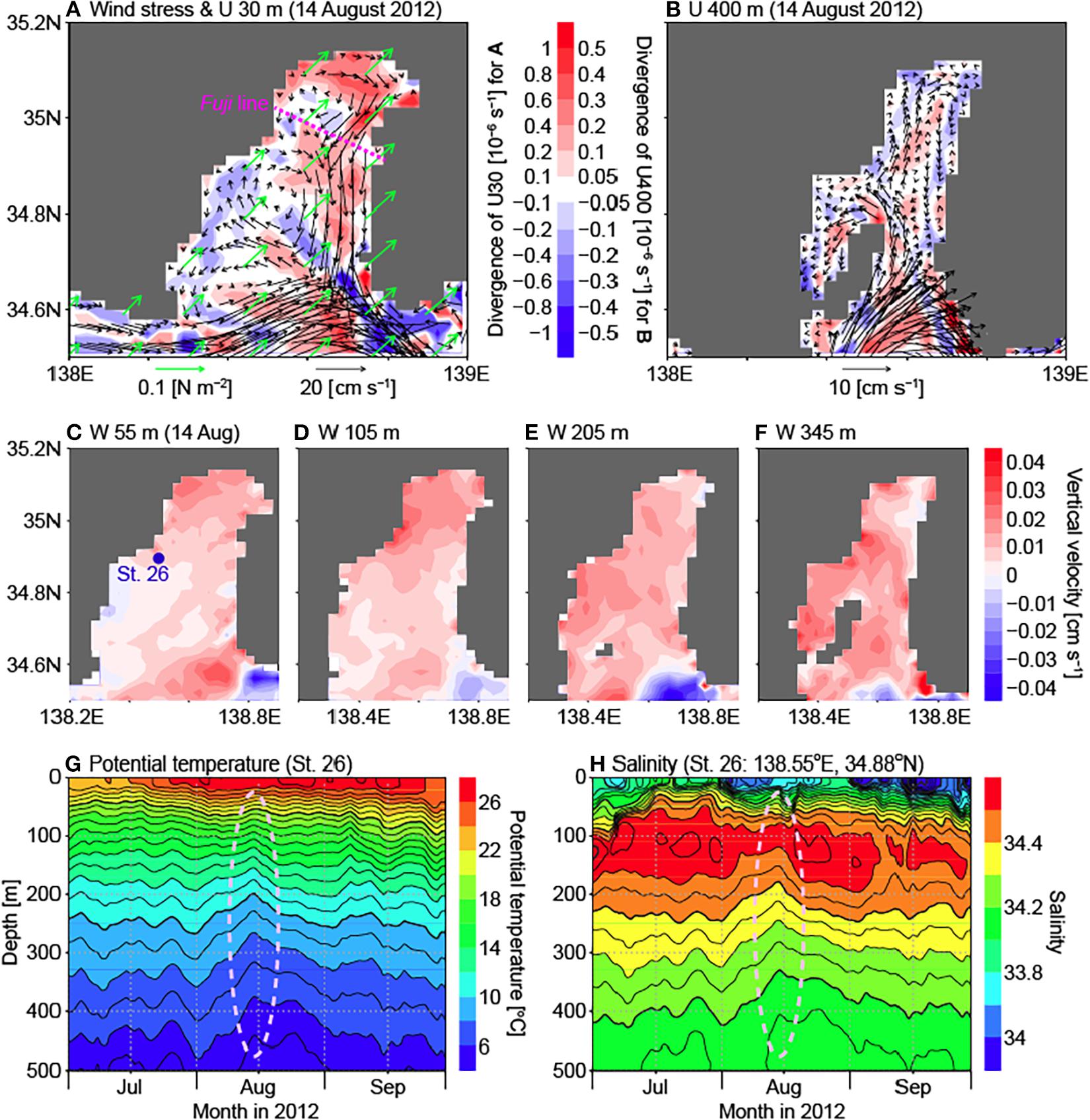
Figure 14. (A) Distributions of surface wind stresses (green arrows), horizontal velocities (black arrows) and horizontal velocity divergences (shading) at 30 m depth. (B) Distributions of horizontal velocities (black arrows) and horizontal velocity divergences (shading) at 400 m depth. (C–F) Distributions of vertical velocities (positive upward) at 55, 105, 205, and 345 m depths, respectively. These distributions (A–F) are for the peak day of the positive EOF3 event, 14 August 2012. (G,H) Time evolutions of potential temperature and salinity profiles at Station 26 of Nakamura (1982) [138.55°E, 34.88°N; blue closed circle in (C)]. Potential temperature and salinity changes during the EOF3 event are indicated by dashed ellipses. Purple dashed line in (A) denotes the ordinary track of the sightseeing ferry Fuji.

Nakamura (1982) reported that temperatures lower than the previous month (“secondary temperature minimum” after the primary temperature minimum in winter) appeared at about 50–200 m depths in the summer of several years during 1964–1974, despite the net surface heating in summer. Nakamura and Uehara (2020) also found that large subsurface cooling consistent with the secondary temperature minimum phenomenon took place in the bay head region based on recent observations during the period 2008–2017; relatively large subsurface cooling was seen in the summer of 2012 in their figures. In the simulation product, time evolutions of potential temperature and salinity profiles (Figures 14G,H) exhibited decreases of potential temperatures and changes of salinities (increases above the salinity maximum at about 100 m depth; decreases below it) in the subsurface layer during the event in the summer of 2012 (dashed ellipses), which were basically consistent with the upwelling as described above. The similarities of our results to the figures as presented in Nakamura (1982) suggested the possibility that the upwelling for compensating the southward divergent flow in the surface layer generated by westerly wind stresses can influence the phenomenon as in the above example. We should note that, since the resolution of the surface forcing field of the simulation product (Tsujino et al., 2018) was about 55 km based on the JRA-55 reanalysis (Kobayashi et al., 2015), surface wind variability on a regional scale (e.g., Kawamura, 1966) was not resolved. Thus, further investigation with forcing fields that resolve the regional variability (e.g., Tanaka et al., 2007, 2008) is necessary for improving the reproduction of the wind-induced circulation in Suruga Bay, which remains for future work. In addition, summertime atmospheric responses to the local SST increases around the Kanto–Tokai district related to the Kuroshio large meander have recently been indicated with an atmospheric model (Sugimoto et al., 2021). Atmospheric feedback should be important for understanding the larger number of positive EOF3 days than negative EOF3 days during the LM period (Figure 4D). Therefore, high-resolution boundary conditions or interacting processes are necessary for both ocean and atmosphere simulations for clarifying and predicting the comprehensive variability in this region. Accumulated hydrographic observation data (e.g., Kutsuwada et al., 2007) would be important data sources for initialization and validation in these modeling studies.

Reproduction of the EOF3 event was validated by using the ADCP data along the regular operation line of the sightseeing ferry Fuji in the bay head region. Figure 15 compares the meridional velocity anomalies along the ferry track line during the EOF3 event. Note that hourly climatology that includes predominant diurnal and semi-diurnal tidal variations as well as seasonal variations (see section “Materials and Methods”) was subtracted for calculating these daily anomalies but qualitatively similar results were obtained (not shown) when we used simple daily averages of available data as in previous studies (e.g., Katsumata et al., 2020). On 11 and 12 August 2012, the observation data indicated southward flow in the central–eastern part and northward flow to the west of 138.6°E approximately in 20–80 m depths. The simulation results basically reproduced this flow structure, although the magnitudes of both southward and northward flows were rather smaller. The EOF3 time coefficient for the simulation result became greater than +1 on 13 August and took a maximum on 14 August; the bay-scale EOF3 flow pattern (Figure 3D) was clear on these days (Figure 15A). At the peak time, southward flow in the surface layer (<100 m depth) with relatively large magnitude (about 14 cm s^–1) was formed at about 138.7°E for both data. On 15 and 16 August, the southward flow weakened and the northward flow in the western part became stronger (in magnitude) than the southward flow. Within the observational limit, the time evolution of the simulation results was basically consistent with the ADCP observations, which lends support to our use of the simulation product. Nevertheless, the differences in details, which can be attributed to errors in calculating interannual anomalies (for both data) and in the parameterizations and forcing of the simulation, should be reexamined in the future for understanding more local-scale variability necessary for fishery use, for example.

FIGURE 15

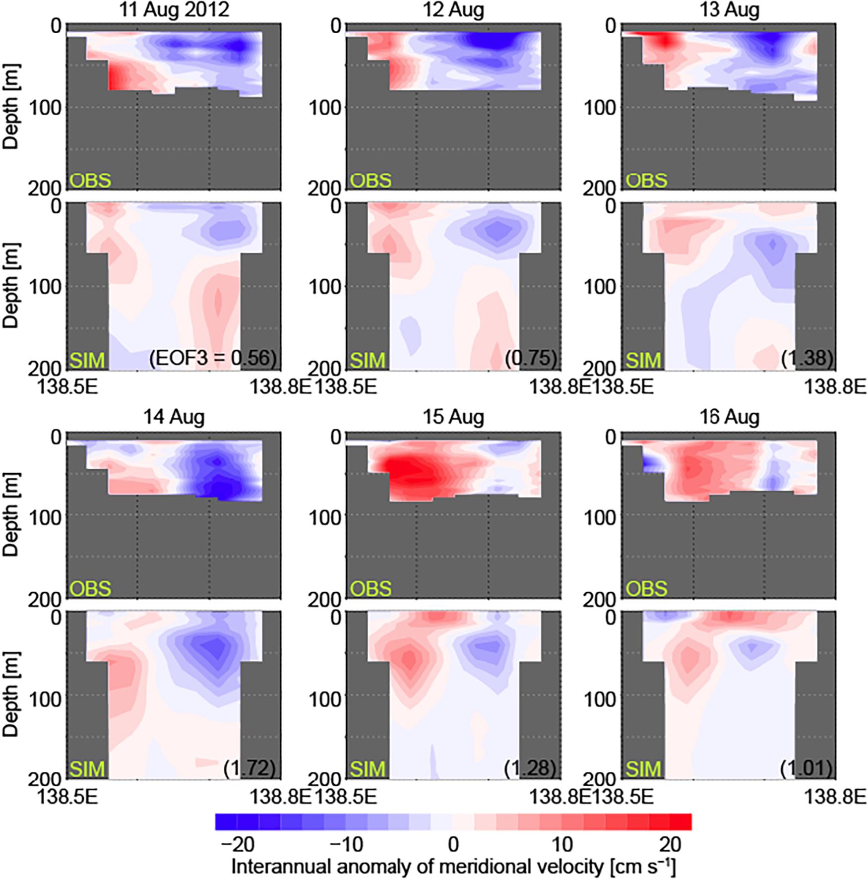
Figure 15. Distributions of daily-mean interannual anomalies of meridional velocities on a cross section along the regular operation line of the sightseeing ferry Fuji (purple dashed line in Figure 14A) between Shimizu Harbor (138.50°E, 35.01°N) and Toi Harbor (138.79°E, 34.91°N) during 11–16 August 2012. ADCP observation data (OBS; upper) and the simulation product (SIM; lower; with EOF3 time coefficient) are compared for each day. Missing values (due to observation limit and land cover) are indicated by gray shading.

The surface-layer flow patterns and related environmental fields as obtained in this study provided useful information for understanding the circulation variability and hence the variabilities in temperature and other properties (e.g., salinity and nutrient) in Suruga Bay. Water exchange between the western boundary current and coastal ocean is one of the key processes in representing these variabilities, which requires reproduction on the horizontal scale ranging from eddies within the bays to the Kuroshio meandering. In this regard, the simulation product used in this study (Hirose et al., 2019) would be an effective tool, resolving bay-scale eddies under the data assimilative constraints on larger scales. Nevertheless, further collaborative feedback between the observational and modeling studies and between the regional and large-scale climate studies is necessary in order to understand the sophisticated interaction processes between scales, which would improve our ability to provide adequate information to society.

Data Availability Statement

Publicly available datasets were analyzed in this study. This data can be found here: https://mri-ocean.github.io/mricom/mri.com-user_jpn_start.html, https://resources. marine.copernicus.eu/?option=com_csw&view=details&product _id=SEALEVEL_GLO_PHY_L4_REP_OBSERVATIONS_008_0 47, https://www.eorc.jaxa.jp/ptree/userguide.html, https://jdoss1. jodc.go.jp/vpage/tide.html.

Author Contributions

TT performed the analysis and wrote the first draft of the manuscript. TT, KT, TK, KK, and TM contributed to the conception and design of this study. KS, NU, and NH contributed to the processing and analysis of the simulation product. KS, HN, LSU, KKK, YK, and GY contributed to the model description, analysis methodology, and interpretation of the model results. TK, DT, MN, and KK contributed to the processing and publication of the shipboard ADCP data. All authors authored the manuscript, contributed to the revision, and approved the final draft.

Funding

This research was supported by the Japan Society for the Promotion of Science (KAKENHI Grants 20H01968 and 19K03978).

Conflict of Interest

The authors declare that the research was conducted in the absence of any commercial or financial relationships that could be construed as a potential conflict of interest.

Publisher’s Note

All claims expressed in this article are solely those of the authors and do not necessarily represent those of their affiliated organizations, or those of the publisher, the editors and the reviewers. Any product that may be evaluated in this article, or claim that may be made by its manufacturer, is not guaranteed or endorsed by the publisher.

Acknowledgments

We are indebted to Hiroyuki Tsujino (Department of Climate and Geochemistry Research, MRI/JMA) who has long been involved in the development of MRI.COM. We are grateful to the reviewers, DK and ZY, for their constructive comments.

Supplementary Material

The Supplementary Material for this article can be found online at: https://www.frontiersin.org/articles/10.3389/fmars.2021.721500/full#supplementary-material

References

Akitomo, K., Awaji, T., and Imasato, N. (1991). Kuroshio path variation south of Japan: 1. Barotropic inflow-outflow model. J. Geophys. Res. 96, 2549–2560. doi: 10.1029/90JC02030

CrossRef Full Text | Google Scholar

Awaji, T., Akitomo, K., and Imasato, N. (1991). Numerical study of shelf water motion driven by the Kuroshio: barotropic model. J. Phys. Oceanogr. 21, 11–27. doi: 10.1175/1520-0485(1991)021<0011:nsoswm>2.0.co;2

CrossRef Full Text | Google Scholar

Hirose, N., Usui, N., Sakamoto, K., Tsujino, H., Yamanaka, G., Nakano, H., et al. (2019). Development of a new operational system for monitoring and forecasting coastal and open-ocean states around Japan. Ocean Dyn. 69, 1333–1357. doi: 10.1007/s10236-019-01306-x

CrossRef Full Text | Google Scholar

Inaba, H. (1981). Circulation pattern and current variations with respect to tidal frequency in the sea near the head of Suruga Bay. J. Oceanogr. Soc. Jpn. 37, 149–159. doi: 10.1007/bf02309052

CrossRef Full Text | Google Scholar

Inaba, H. (1982). Relationship between the oceanographic conditions of Suruga Bay and locations of the Kuroshio path. Bull. Coast. Oceanogr. 19, 94–102.

Google Scholar

Inaba, H. (1984). Current variation in the sea near the mouth of Suruga Bay. J. Oceanogr. Soc. Jpn. 40, 193–198. doi: 10.1007/bf02302552

CrossRef Full Text | Google Scholar

Inaba, H. (1988). Oceanographic environment of Suruga Bay. Bull. Jpn. Soc. Fish. Oceanogr. 52, 236–240.

Google Scholar

Inaba, H., Katsumata, T., and Yasuda, K. (2001). Temporal variations of current and temperature at 300 m in Suruga Bay. Deep Ocean Water Res. 2, 1–8.

Google Scholar

Iwata, T., Shinomura, Y., Natori, Y., Igarashi, Y., Sohrin, R., and Suzuki, Y. (2005). Relationship between salinity and nutrients in the subsurface layer in the Suruga Bay. J. Oceanogr. 61, 721–732. doi: 10.1007/s10872-005-0079-2

CrossRef Full Text | Google Scholar

Katsumata, T. (2004). Intrusion Process of Oceanic Water to Suruga Bay. Ph.D. thesis. (Shizuoka: Tokai University), 110.

Google Scholar

Katsumata, T. (2016). Generation of periodic intrusions at Suruga Bay when the Kuroshio follows a large meandering path. Cont. Shelf Res. 123, 9–17. doi: 10.1016/j.csr.2016.04.005

CrossRef Full Text | Google Scholar

Katsumata, T., Niki, M., Tanaka, A., Tan, H., Takashima, K., Takahashi, D., et al. (2020). The current of the inner part of Suruga Bay in 2008 – The current observation by using acoustic Doppler current profiler (ADCP) mounted on the Suruga-wan ferry. Bull. Inst. Oceanic Res. Dev. 42, 15–24.

Google Scholar

Kawabe, M. (1986). Transition processes between the three typical paths of the Kuroshio. J. Oceanogr. Soc. Jpn. 42, 174–191. doi: 10.1007/BF02109352

CrossRef Full Text | Google Scholar

Kawabe, M. (1995). Variations of current path, velocity and volume transport of the Kuroshio in relation with the large meander. J. Phys. Oceanogr. 25, 3103–3117. doi: 10.1175/1520-0485(1995)025<3103:vocpva>2.0.co;2

CrossRef Full Text | Google Scholar

Kawabe, M. (2005). Variations of the Kuroshio in the southern region of Japan: conditions for large meander of the Kuroshio. J. Oceanogr. 61, 529–537. doi: 10.1007/s10872-005-0060-0

CrossRef Full Text | Google Scholar

Kawamura, T. (1966). Surface wind systems over central Japan in the winter season. Geogr. Rev. Jpn. 39, 538–554. doi: 10.4157/grj.39.538

CrossRef Full Text | Google Scholar

Kimura, K. (1950). Investigation of ocean current by drift-bottle experiments (No. 1)—Current in Suruga Bay with special reference to its anti-clockwise circulation within the bay. J. Oceanogr. Soc. Jpn. 5, 70–83.

Google Scholar

Kobayashi, S., Ota, Y., Harada, Y., Ebita, A., Moriya, M., Onoda, H., et al. (2015). The JRA-55 Reanalysis: general specifications and basic characteristics. J. Meteorol. Soc. Jpn. 93, 5–48. doi: 10.2151/jmsj.2015-001

PubMed Abstract | CrossRef Full Text | Google Scholar

Kurihara, Y., Murakami, H., and Kachi, M. (2016). Sea surface temperature from the new Japanese geostationary meteorological Himawari-8 satellite. Geophys. Res. Lett. 43, 1234–1240. doi: 10.1002/2015GL067159

CrossRef Full Text | Google Scholar

Kurihara, Y., Sakurai, T., and Kuragano, T. (2006). Global daily sea surface temperature analysis using data from satellite microwave radiometer, satellite infrared radiometer and in-situ observations. Weather Bull. 73, 1–18.

Google Scholar

Kutsuwada, K., Tanikawa, M., Hagiwara, Y., and Katsumata, T. (2007). Long-term variability of upper oceanic condition in Suruga Bay and its surrounding area. Oceanogr. Jpn. 16, 277–290.

Google Scholar

Mertz, F., Pujol, M. I., and Faugère, Y. (2018). Product User Manual for Sea Level SLA Products. CMEMS-SL-PUM-008-032-051, COPERNICUS Marine and Environment Monitoring Service. Available online at: https://resources.marine.copernicus.eu/documents/PUM/CMEMS-SL-PUM-008-032-051.pdf (accessed August 13, 2019).

Google Scholar

Miyama, T., and Miyazawa, Y. (2014). Short-term fluctuations south of Japan and their relationship with the Kuroshio path: 8- to 36-day fluctuations. Ocean Dyn. 64, 537–555. doi: 10.1007/s10236-014-0701-1

CrossRef Full Text | Google Scholar

Miyama, T., Miyazawa, Y., Varlamov, S., and Hihara, T. (2018). Development of the Kuroshio large meander in 2017. Kaiyo Monthly 50, 107–113.

Google Scholar

Nakamura, M., and Uehara, K. (2020). Multi-Layer Temperature Variability at Kurasawa on the Back of Suruga Bay. JpGU–AGU Joint Meeting 2020, AOS18-AOS17. Available online at: https://confit.atlas.jp/guide/event/jpgu2020/subject/AOS18-P07/detail

Google Scholar

Nakamura, Y. (1972). Hydrographic studies in Suruga Bay, II—The flowing at the surface in the inner part. Bull. Coast. Oceanogr. 9, 44–53.

Google Scholar

Nakamura, Y. (1982). Oceanographic feature of Suruga Bay from view point of fisheries oceanography. Bull. Shizuoka Pref. Fish. Exp. Stn. 17, 1–153.

Google Scholar

Nakamura, Y., and Muranaka, H. (1979). Temporal fluctuation of oceanographic structure in Suruga Bay and Enshu-Nada. Bull. Jpn. Soc. Fish. Oceanogr. 34, 128–133.

Google Scholar

Niki, M., Katsumata, T., and Sugimoto, T. (2014). Study on the estimation of harmonic analysis method using ADCP data measured by regular ferry. J. Jpn. Soc. Civil Eng. 70, I_486–I_490. doi: 10.2208/kaigan.70.I_486

CrossRef Full Text | Google Scholar

Niki, M., Sugimoto, T., Katsumata, T., and Sakaguchi, A. (2011). Field observation for spreading of Fuji River water in the inner part of Suruga Bay. J. Jpn. Soc. Civil Eng. 67, I_346–I_350. doi: 10.2208/kaigan.67.I_346

CrossRef Full Text | Google Scholar

Ramp, S. R., Barrick, D. E., Ito, T., and Cook, M. S. (2008). Variability of the Kuroshio Current south of Sagami Bay as observed using long-range coastal HF radars. J. Geophys. Res. 113:C06024. doi: 10.1029/2007JC004132

CrossRef Full Text | Google Scholar

Sato, K. (1967). On the sea conditions in Suruga Bay. (Tokyo: Maritime Safety Agency), 124.

Google Scholar

Sugimoto, S., Qiu, B., and Kojima, A. (2020). Marked coastal warming off Tokai attributable to Kuroshio large meander. J. Oceanogr. 76, 141–154. doi: 10.1007/s10872-019-00531-8

CrossRef Full Text | Google Scholar

Sugimoto, S., Qiu, B., and Schneider, S. (2021). Local atmospheric response to the Kuroshio large meander path in summer and its remote influence on the climate of Japan. J. Clim. 34, 3571–3589. doi: 10.1175/JCLI-D-20-0387.1

CrossRef Full Text | Google Scholar

Takeuchi, K., and Hibiya, T. (1997). Numerical simulation of baroclinic tidal currents in Suruga Bay and Uchiura Bay using a high resolution level model. J. Oceanogr. 53, 539–552.

Google Scholar

Tanaka, K., Michida, Y., and Komatsu, T. (2007). A numerical experiment on ocean circulations forced by seasonal winds in Suruga Bay. Coast. Mar. Sci. 31, 30–39.

Google Scholar

Tanaka, K., Michida, Y., and Komatsu, T. (2008). Numerical experiments on wind-driven circulations and associated transport processes in Suruga Bay. J. Oceanogr. 64, 93–102. doi: 10.1007/s10872-008-0007-3

CrossRef Full Text | Google Scholar

Tanaka, K., Michida, Y., and Komatsu, T. (2010). Impact of sporadically enhanced river discharge on the climatological distribution of river water in Suruga Bay. Coast. Mar. Sci. 34, 1–6.

Google Scholar

Tanaka, K., Michida, Y., Komatsu, T., and Ishigami, K. (2009). Spreading of river water in Suruga Bay. J. Oceanogr. 65, 165–177. doi: 10.1007/s10872-009-0016-x

CrossRef Full Text | Google Scholar

Tsujino, H., Nakano, H., Sakamoto, K., Urakawa, S., Hirabara, M., Ishizaki, H., et al. (2017). Reference manual for the Meteorological Research Institute Community Ocean Model version 4 (MRI.COMv4). Tech. Rep. 80. Tsukuba: Meteorological Research Institute. doi: 10.11483/mritechrepo./80

CrossRef Full Text | Google Scholar

Tsujino, H., Urakawa, S., Nakano, H., Small, R. J., Kim, W. M., Yeager, S. G., et al. (2018). JRA-55 based surface dataset for driving ocean-sea-ice models (JRA55-do). Ocean Modell. 130, 79–139. doi: 10.1016/j.ocemod.2018.07.002

CrossRef Full Text | Google Scholar

Usui, N., Tsujino, H., Nakano, H., and Matsumoto, S. (2013). Long-term variability of the Kuroshio path south of Japan. J. Oceanogr. 69, 647–670. doi: 10.1007/s10872-013-0197-1

CrossRef Full Text | Google Scholar

Usui, N., Wakamatsu, T., Tanaka, Y., Hirose, N., Toyoda, T., Nishikawa, S., et al. (2017). Four-dimensional variational ocean reanalysis: a 30-year high-resolution dataset in the western North Pacific (FORA-WNP30). J. Oceanogr. 73, 205–233. doi: 10.1007/s10872-016-0398-5

CrossRef Full Text | Google Scholar