 Ziyu Xiao
 Zhaoqing Yang
 Taiping Wang
 Ning Sun
 Mark Wigmosta2,3
 David Judi
- 1Pacific Northwest National Laboratory, Coastal Sciences Division, Seattle, WA, United States
- 2Department of Civil and Environmental Engineering, University of Washington, Seattle, WA, United States
- 3Pacific Northwest National Laboratory, Earth Sciences Division, Richland, WA, United States
Low-lying coastal areas in the mid-Atlantic region are prone to compound flooding resulting from the co-occurrence of river floods and coastal storm surges. To better understand the contribution of non-linear tide-surge-river interactions to compound flooding, the unstructured-grid Finite Volume Community Ocean Model was applied to simulate coastal storm surge and flooding in the Delaware Bay Estuary in the United States. The model was validated with tide gauge data in the estuary for selected hurricane events. Non-linear interactions between tide-surge-river were investigated using a non-stationary tidal analysis method, which decomposes the interactions’ components at the frequency domain. Model results indicated that tide-river interactions damped semidiurnal tides, while the tide-surge interactions mainly influenced diurnal tides. Tide-river interactions suppressed the water level upstream while tide-surge interaction increased the water level downstream, which resulted in a transition zone of damping and enhancing effects where the tide-surge-river interaction was prominent. Evident compound flooding was observed as a result of non-linear tide-surge-river interactions. Furthermore, sensitivity analysis was carried out to evaluate the effect of river flooding on the non-linear interactions. The transition zone of damping and enhancing effects shifted downstream as the river flow rate increased.
Introduction
Coastal flooding hazards caused by tropical cyclones present a severe risk to nearly 40% of the U.S. population living in low-lying coastal areas. The co-occurrence of storm surge and river flooding may cause compound flooding (Bevacqua et al., 2019), which results in extreme water levels caused by non-linear interactions of storm surges, river flood, and astronomical tides (Doodson, 1956; Proudman, 1957; Rossiter, 1961; Johns et al., 1985; Arns et al., 2020). Coastal flood risks associated with compound flooding cannot be simply estimated by superposition of astronomical tides and river-induced and storm-surge-induced water levels. Non-linear interactions are known to exist between tides, storm surge, and river flow, but understanding of how non-linear interactions exacerbate the compounding effect is limited. The total water levels could be increased or decreased by the non-linear interactions between storm surges, river flow, and tides. Furthermore, such non-linear interaction is sensitive to sea level rise, storm intensity, and river flow as a result of climate change (Yang et al., 2014; Li et al., 2020), which makes the flood hazard risk even more complex and unpredictable.
The characteristics and mechanisms of tide-surge interactions (TSIs) have been widely studied during recent decades (Proudman, 1955; Prandle and Wolf, 1978; Wolf, 1978; Idier et al., 2012; Zhang et al., 2020). In an early study conducted in the North Sea and River Thames, United Kingdom, observed TSI was found to amplify surge height significantly on rising tides, independent of initial surge height or the relative phase difference between tides and surges (Proudman, 1955). Horsburgh and Wilson (2007) gave a first-order explanation of the surge cluster that occurs with rising tide based on the phase shift of the tidal signal (the effect of surge on tides) combined with the modulation of surge production due to the change in water depth (the effect of tides on surge). Olbert et al. (2013) applied a statistical method to the hindcast over 1959–2005 in the Irish Sea and found that surges tend to peak at a particular phase of tide irrespective of the timing of the storm landfall but with site specificity. The degree of total water level modulation due to TSI is also site-specific and varies with surge height and tidal ranges (Keers, 1968; Prandle and Wolf, 1978). Prandle and Wolf (1978) used a one-dimensional model to show that TSI is mainly produced by the quadratic friction effect followed by the shallow water and advective effects, and that the shallow water and advective effects can be dominant on rising tides, while quadratic friction can be prominent on high tides.
Tides that propagate into the upper estuaries are subject to tide-river interactions (TRIs), resulting in the modulation of tidal amplitudes at specific tidal frequencies by bottom friction and river flow (Godin, 1999; Horrevoets et al., 2004). Based on the shallow water equation, TRI can be caused by three non-linear terms: spatial acceleration, friction, and a gradient of river flow (Dronkers, 1964). The TRI between river flow and tides has been demonstrated to attenuate tidal energy in the upstream of an estuary, while it stimulates energy transfer from the principal tides to overtides in the downstream (Guo et al., 2015). However, the variation in TRI corresponding to varying river flow and its damping effect on total water level have not been described in detail.
Tide-surge-river interactions (TSRIs) are the non-linear interactions among tides, storm surge and river flow, which add additional complexity to TSIs due to the presence of storm surge and river flooding. Although TSRIs are rarely studied, they are an important component of storm surges. For example, Dinapoli et al. (2021) found that the current due to river flow (CDR) non-linearly interacts with both the tides and storm surges in the Río de la Plata estuary. Their work further suggests the tide-CDR and surge-CDR interactions both induce asymmetries in the water level and the interactions are mainly caused by the quadratic bottom friction. Spicer et al. (2019) and Spicer et al. (2021) collected observations in Maine estuaries during “windstorms” and pointed out the TSRI to be the dominant mechanism contributing to upstream surge amplification (which is estimated to be exceeding 1m and more than double than non-tidal forcing induced surges). By testing different combinations of the atmospheric forcing effect on generating the extreme water levels via non-stationary tidal harmonic analysis (Matte et al., 2013), the mechanism to generate TSRI is found to be related to the increased mean flow and frictional energy from wind forcing (Spicer et al., 2021). A comprehensive review on different interaction mechanisms between SLR-tide-surge, tide-surge, tide-river, wave-surge, tide-wave, and SLR-wave was conducted along the coasts and estuaries worldwide (Idier et al., 2019), the values of the interactions vary from a few tens of centimeters to over 1 m.
Many previous studies focused on TSI or TRI independently. However, during compound flooding events when extreme surge levels co-occur with extreme river flooding, both TSI and TRI modulate the total water levels (TWLs) as part of TSRI. To the authors’ knowledge, the relative importance of TSI and TRI to the overall TSRI during compound flooding events has not been well documented. Spicer et al. (2019) raised attention to the importance of distinguishing how non-linear TRI varies from TSI by using a non-stationary tidal analysis method to account for non-linear interactions. The methods to analyze tidal constituents of a tidal record have been well summarized by Hoitink and Jay (2016), based on assumptions of either stationary or non-stationary environments. The traditional stationary methods, such as harmonic analysis (Pawlowicz et al., 2002), assume that tidal constituents are fixed and independent from oceanic and atmospheric forcings, thus appropriate for tides in the deep ocean (Dean, 1966; Godin, 1972; Flinchem and Jay, 2000). For tides affected by rivers and coastal processes, the non-stationary method can resolve the time-changing tidal amplitude and phase due to strong non-linear interactions between atmospheric forcing, river flow, and tides (Jay and Flinchem, 1997; Matte et al., 2013, 2014; Sassi and Hoitink, 2013; Guo et al., 2015). Jalón-Rojas et al. (2018) compared the advantages and disadvantages of stationary and non-stationary methods used in tidal analysis and concluded that the stationary method does not reproduce the time-varying properties of the tidal signal and therefore cannot be used to predict the non-linear interactions between tidal constituents and non-tidal forcing variations; however, the non-stationary method can be used to distinguish non-linear components. Lastly, although the effects of wind waves and wave-current interaction could have additional impact on storm surge, we decided not to explicitly include wind waves in this study due to two main reasons. First, in a recent study by Ye et al. (2020) using a comprehensive hydrodynamic model framework that includes wind waves, the authors fund that the effect of wave-current interaction on storm surge is very small (i.e., a few centimeters) inside Delaware Bay during Hurricane Irene. Second, we feel it is important to first elucidate the effects of TSRIs on storm surge before further expand the scope to include more processes, which include wind waves and baroclinic processes. On the other hand, studies by Sheng et al. (2010) and Hsiao et al. (2019) also suggested that wave-induced setup could contribute significantly to the storm surge elevation, depending on specific study sites and hurricane/typhoon events. Thus, to explicitly include wind waves should be considered in the next phase of modeling work.
Numerical model simulations offer good insights to help isolate each interaction process and estimate the uncertainty of flooding risk caused by the complexity of non-linear interactions. This paper presents the results of a modeling study conducted to investigate the variations between TRI, TSI, and TSRI and evaluate their interactions and their contributions to the TWL during compound flooding events in the Delaware Bay Estuary (DBE). By comparing non-linear terms produced during selected historical hurricane events, this study characterized the damping and amplification effects of different non-linear interaction processes on TWL and analyzed the underlying mechanisms. The non-stationary tidal analysis method was applied to quantify the relative contribution by diurnal, semidiurnal, and quarter-diurnal tidal bands to the non-linear interactions. In addition, the sensitivity of non-linear interaction to different return period river flows was explored.
Methodology
Study Site
The funnel-shaped DBE is located on the mid-Atlantic coast of the United States (Figure 1A). The estuary mouth is about 18 km wide and the bay has a maximum width of 45 km in the lower bay and converges to a width of 0.3 km at Trenton (Figure 1B), stretching about 210 km toward the head of a tidal freshwater river (Sharp, 1984). Mean estuary depth is 7 m, the deepest waters exceed 30 m, and a shipping channel has been progressively deepened since the late 1800s by increasing the thalweg of the estuary from roughly 8 to 15 m (Pareja Roman, 2019). The DBE is dominated by semidiurnal tides where M2 and S2 tides account for up to 96% of the tidal variability (Aristizabal and Chant, 2013), which is strongly convergent and moderately dissipative in terms of tidal energy (Lanzoni and Seminara, 1998). The tidal range is approximately 1.5 m at the estuary mouth and is amplified upstream; the maximum tidal current is approximately 1 m/s (Wong and Sommerfield, 2009). The Delaware River provides more than half of the freshwater discharge to the estuary (Whitney and Garvine, 2006). A hydraulic jump is observed ~2.7 km downstream of the Trenton tidal gauge (Figure 1B) due to the abrupt transition in bathymetry and roughly represents the upstream limit of tidal intrusion (Zhang et al., 2020).
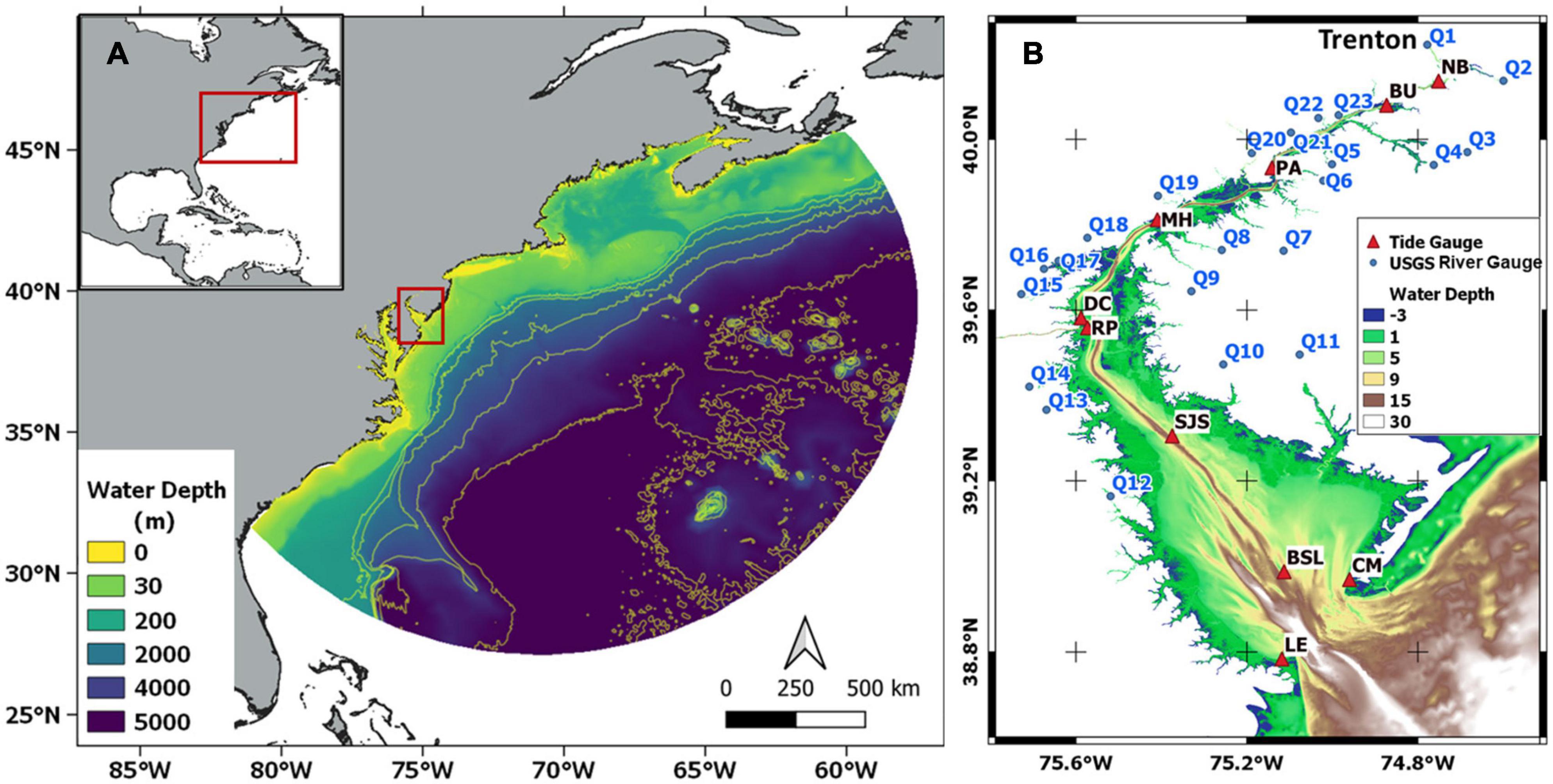
Figure 1. (A) Model domain and bathymetry. (B) 10 NOAA tidal gauges and 23 U.S. Geological Survey river gauges with bathymetry inside the DBE. The 10 tide gauges in the DBE are listed as Lewes (LE), Cape May (CM), Brandywine Shoal Light (BSL), Ship John Shoal (SJS), Reedy Point (RP), Delaware City (DC), Marcus Hook (MH), Philadelphia (PA), Burlington (BU), and Newbold (NB).
Delaware Bay Estuary is undammed along its main stem and has networks of tidal flats that store vegetation, sediment, and nutrients in the lower bay. DBE provides a natural testbed for examining the mechanisms and characteristics of non-linear interactions among different physical processes under extreme storm conditions.
Numerical Model
The numerical model used in this study is the unstructured-grid, Finite-Volume Community Ocean Model (FVCOM) (Chen et al., 2003). FVCOM has been used extensively for modeling storm surge in many coastal regions worldwide (Song et al., 2013; Chen et al., 2014, 2016; Wang and Yang, 2019; Yang et al., 2021). The unstructured-grid framework allows the flexibility to robustly simulate fine-scale dynamic processes in any complex estuarine and coastal bay system. In this study, an unstructured-grid for the DBE was developed to cover a model domain that extends ~1500 km offshore from the coast and ~240 km upstream from the DBE mouth (Figure 2). The model grid consisted of 822,684 triangle elements and 429,847 nodes. The unstructured-grid resolution varies from 40 km at the open boundary to approximately 100 m in the estuary, and the highest resolution of 20 m is for tributaries. The average grid resolution for the floodplain is approximately 100 m. The land boundary of floodplain is cut off at 3 m above the mean sea level to allow for simulation of inland inundation. A sigma-stretched vertical coordinate of five layers was used for all the model runs. The wetting and drying algorithm, which incorporates a bottom viscous layer of specified thickness (Dmin = 5 cm in the present study), was applied to simulate the inundation process in the intertidal zone and floodplain.
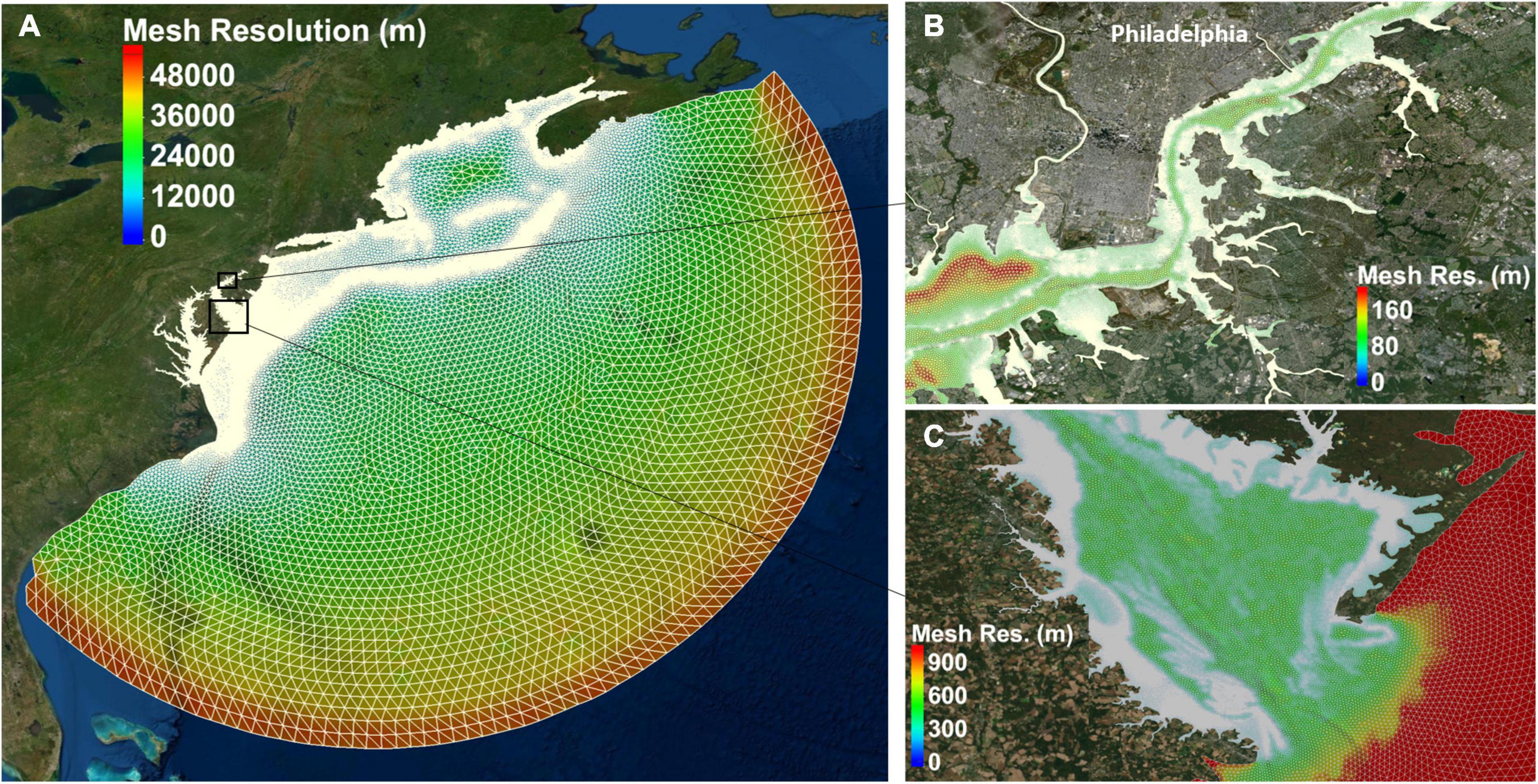
Figure 2. FVCOM model grid (white line) with color contours showing the mesh resolution (A) the whole model domain (B) zoom-in of the upper channel near Philadelphia (C) lower bay near estuary mouth.
Model open-boundary conditions were specified by tidal elevations obtained from the TPXO8.0 global ocean tide model1. Sea surface wind field was obtained from the global atmospheric reanalysis model European Centre for Medium-Range Weather Forecasts (ECMWF) Reanalysis v5 (ERA5), which has a spatial resolution of 30 km and temporal resolution of 1 hr. River flows collected at 23 U.S. Geological Survey (USGS) river gauges in the DBE were specified as the river boundary condition (Figure 1). The main rivers discharged into DBE are the Delaware River (Q1) and Schuylkill River (Q20), which, respectively, contribute about 58% and 14% of the total freshwater inflow (Sharp, 1984). Sensitivity tests of bottom roughness conducted by Ye et al. (2020) suggested that a spatially varying bottom roughness is necessary to represent the different bottom characteristics in the lower and upper bay. In this study, bottom roughness was calibrated based on observed M2 amplitude at ten tidal gauges. Initial bottom roughness values of 0.0001 and 0.0025 m were tested for the entire domain. Final bottom roughness values of 0.0005 m for the coastal ocean to lower bay and 0.0001 m for the middle and upper bay were specified, which gave good calibration results (Figure 3).
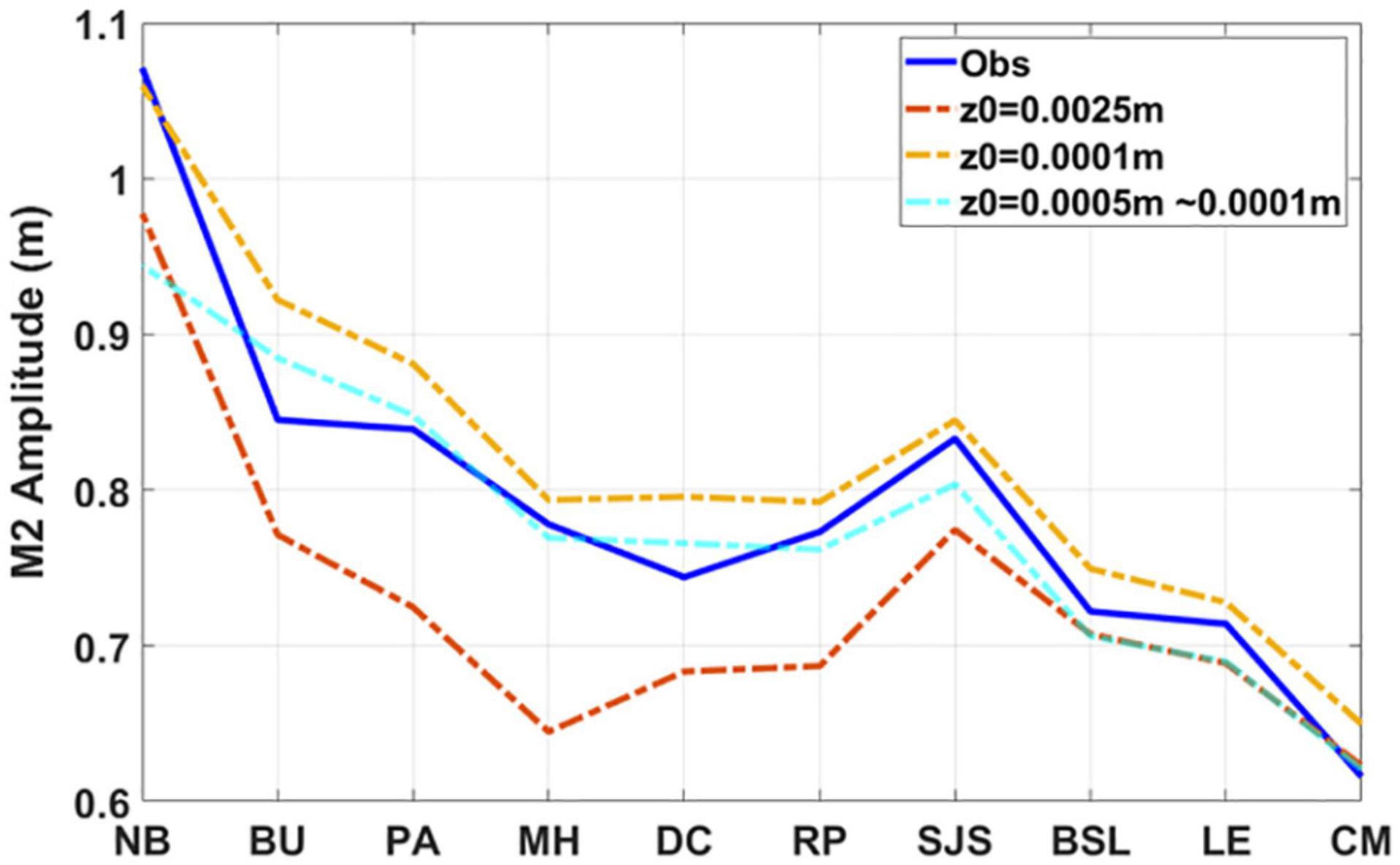
Figure 3. Model calibration of bottom roughness based on M2 tidal amplitude.
The model bathymetry was interpolated based on four different bathymetry data sets from the National Oceanic and Atmospheric Administration (NOAA): (a) 1/9 arc-second resolution (~3.5 m) Continuously Updated Digital Elevation Model (CUDEM, doi: 10.25921/ds9v-ky35), which covers the DBE; (b) the 1/3 arc-second (~10 m) and 1 arc-sec (~30 m) data from the National Centers for Environmental Information (NCEI), which covers the nearshore coastal areas; (c) 3 arc-sec (~90 m) Coastal Relief Model2 for the less than 300 m deep coastal waters and floodplain; and (d) the 1 arc-min ETOPO1 Global Relief Model (Amante and Eakins, 2009) for the deep ocean. The model vertical datum was referenced to the North American Vertical Datum of 1988 (NAVD88) and any data set that had a different vertical datum was converted to NAVD88 using V-Datum program (Parker et al., 2003; Yang et al., 2008).
TWL and Non-linear Interaction Decomposition
To characterize the non-linear interaction, time series of TWLs were decomposed into astronomical tides, low-frequency surge (LFSs), and non-linear interactions, following the method of Spicer et al. (2019), Spicer et al. (2021). Astronomical tides were obtained from the Tide Only (TO) model run (Table 1). LFS represents the water level setup induced by non-tidal forcing, such as river flow, surface wind, and atmospheric pressure. The total surge level (TSL), which consists of LFS and non-linear interaction, was obtained by subtracting astronomical tides from TWL. LFS was extracted from TSL using a low-pass filter with a cut-off frequency of 35 hr to remove tidal signals (Walters and Heston, 1982). The non-linear interaction was calculated by subtracting LFS from TSL. Figure 4 details the flowchart to decompose the time series of TWL and obtain the non-linear interaction term. The method was first applied at the 10 tidal gauges (Figure 1B) for model calibration and then applied to the whole model domain.
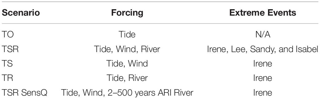
Table 1. Design of numerical experiments for non-linear interactions analysis.
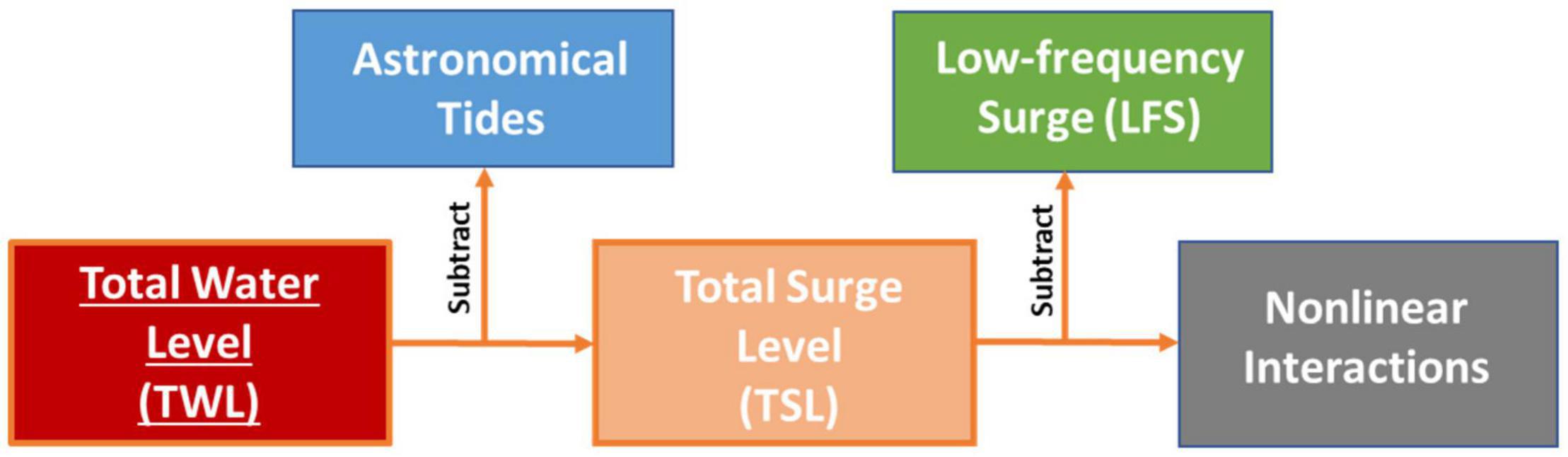
Figure 4. Flowchart of decomposing the TWL into tides, low-frequency surge, and non-linear interactions. TWL = Tides + LFS + Non-linear Interactions.
To understand the process of non-linear interaction with tides, the non-linear interaction term is further decomposed based on its specific tidal frequency. A non-stationary tidal analysis method—Complex Demodulation (Gasquet and Wootton, 1997; Jalón-Rojas et al., 2018)—was applied to a non-linear interaction term to estimate the time-dependent amplitude and phase of diurnal (D1), semidiurnal (D2), and high-frequency (D4, D6, and D8) tidal bands. Complex demodulation is based on a wavelet approach and assumes that the time series X(t) is composed of an oscillating signal with frequency σ and a non-periodic signal Z(t):
where, tidal frequency σ is calculated as 2π/24 rad h–1 for D1, 2π/12.4206 rad h–1 for D2, 2π/6.21 rad h–1 for D4, 2π/4.14 rad h–1 for D6, and 2π/3.10 rad h–1 for D8; time-dependent amplitude A and phase ∅ can be calculated by integrating the frequency σ with respect to time following the steps below (Jalón-Rojas et al., 2018):
a) The time series X(t) is multiplied by a complex modulation of frequency e−iσt to get an unfiltered modulated signal in order to shift the frequency of interest to zero:
b) Y(t) is low-pass filtered to remove frequencies at or above σ,whereas the terms are removed, thus the oscillation in the original signal X(t) is effectively removed to get:
c) The time-varying amplitude A′(t) and phase ∅′(t) are calculated from the Inverse Fourier Transform (Bloomfield, 2004) of the filtered spectrum Y′ (t) by taking twice the magnitude of Y′ (t) and the arc tangent of the ratio of the imaginary to real parts of Y′ (t), respectively.
In addition to the wavelet transform method, a spectral technique—the so called singular spectral analysis (SSA) method—is also presented in this study. This method has been demonstrated to be especially efficient for extracting information from short and noisy time series without previous knowledge of the non-linear dynamics affecting the time series (Schoellhamer, 2001, 2002). The SSA method is widely used to quantify the relative contributions made by different processes to the total variance of the time series (Jalón-Rojas et al., 2016, 2017; Xiao et al., 2020). The SSA method decomposes a time series into so-called reconstructed components by sliding a window of width M down the time series and obtaining an autocorrelation matrix (Vautard et al., 1992). The eigenvalues of the autocorrelation matrix give the contribution of each period to the total variance of the analyzed time-series data set. For further information about the SSA method, the reader is referred to Vautard et al. (1992). Jalón-Rojas et al. (2016) state that a combined approach of wavelet transform method and SSA for short-term analysis complement each other. SSA complements the wavelet transform method in terms of quantification, and the wavelet transform method complements SSA by reconstructing and visualizing the time series of interested periods.
Model Validation and Simulations
Extreme Events and Numerical Experiments Design
The major historical hurricanes since 2000 that have affected the DBE include Isabel (2003), Hurricane Irene (2011), and Hurricane Sandy (2012). Tropical Storms Lee (2011), which followed Hurricane Irene, also brought heavy rainfall to the Delaware River Basin. These extreme events were selected to validate the storm surge model of the DBE Figure 5 shows the tracks of these hurricanes obtained from the hurricane database (HURDAT) at National Hurricane Center (Landsea and Franklin, 2013).
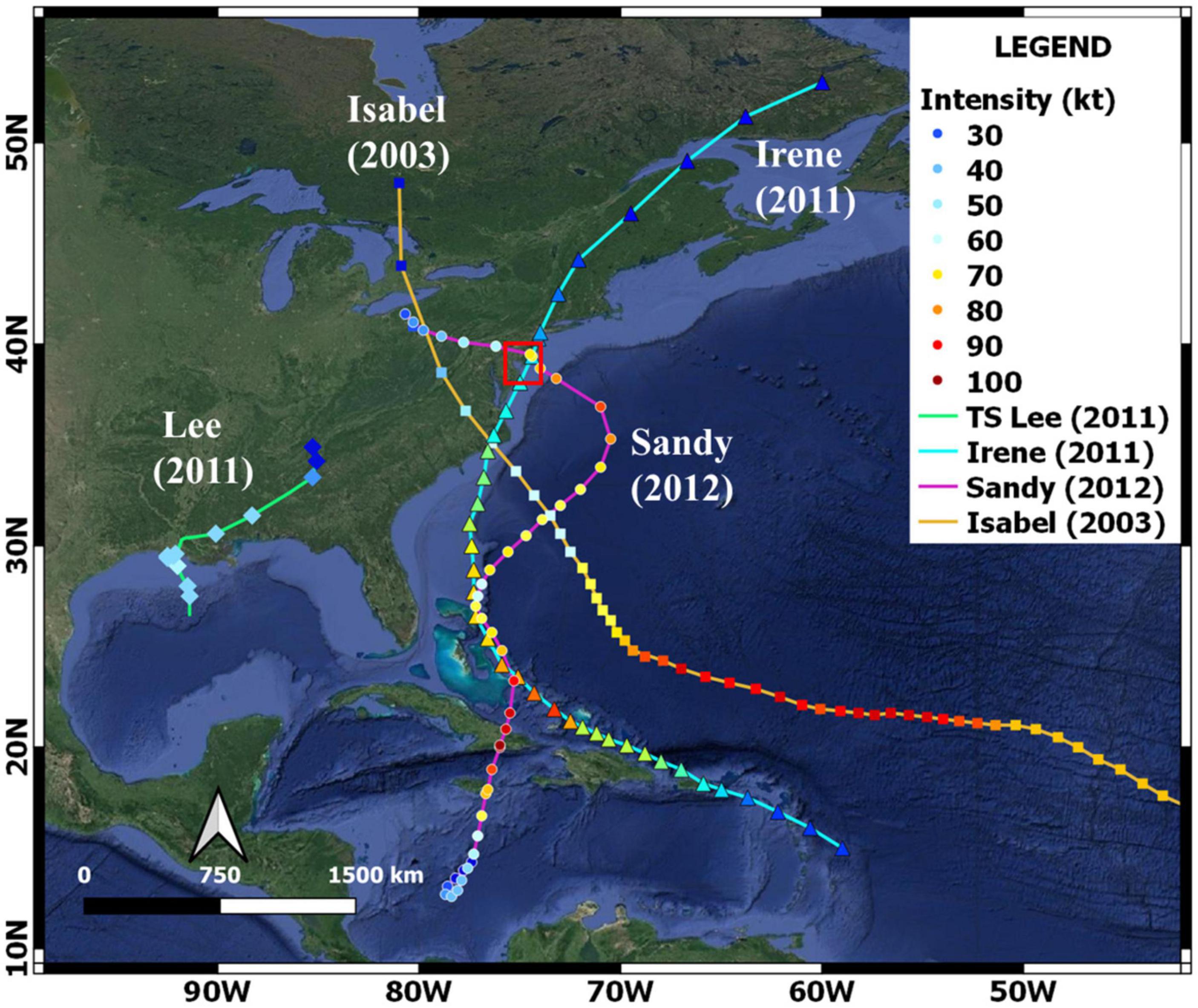
Figure 5. Tracks of selected hurricane and tropical storm events – Isabel (2003), Irene and Lee (2011), and Sandy (2012). Red box indicates the DBE.
Hurricane Isabel was formed on September 1, 2003 and intensified to a category 5 hurricane on September 11, 2003, with a maximum sustained wind speed of 145 kts. It made landfall near the banks of North Carolina at 17:00 UTC September 18. 2003, as a slow-moving system, and proceeded on a northwesterly track (Figure 5). Isabel produced storm surges of 1.8 m to 2.4 m above normal tides near the point of landfall along the Atlantic coast of North Carolina, with reduced storm surge levels ranging from 0.6 m to 1.2 m along Delaware shorelines.
Hurricane Sandy, one of the largest Atlantic hurricanes on record, made landfall as an extratropical cyclone near New Jersey at 23:30 UTC October 29, 2012, and proceeded on a northeasterly track (Figure 5). The maximum sustained wind speed was estimated to be 100 kts and the storm surge peak was 0.9 m to 1.5 m along Delaware shorelines.
Hurricane Irene, one of the costliest hurricanes on record in the U.S., made primary landfall along the US East Coast on the North Carolina shoreline as a category 1 hurricane at 12:00 UTC on August 27, 2011, and another landfall at 09:35 UTC on August 28, 2011, near New Jersey, and continued along the Atlantic coastline (Figure 5). The maximum sustained wind speed was about 105 kts and peak storm surges were between 1.2 and 1.8 m along the coast of New Jersey. Hurricane Irene is an example of a compound flooding event during which the combination of storm surge and rainfall-induced freshwater river flooding amplifies the hazardous impacts of individual events (Ye et al., 2020).
Tropical Storm Lee formed over the Gulf of Mexico (Figure 5) and made landfall along the coast of southern Louisiana at 10:30 UTC on September 3, 2011. The strongest wind (60 kts) associated with the low pressure occurred primarily over the northern Gulf of Mexico. Lee brought heavy rainfall to the Mid-Atlantic region, which caused some of the most severe flooding in the region’s history.
Two large precipitation events associated with Hurricane Irene and Tropical Storm Lee resulted in two peak flows from Delaware River up to 4000 m3/s and 5500 m3/s on August 28, 2011 and September 9, 2011 at Trenton (USGS, 1463500, Figure 6A). The peak flows during Hurricanes Isabel and Sandy were less significant than those during Hurricane Irene and Tropical Storm Lee, which measured up to 1500 m3/s (Figure 6B) and 800 m3/s at Trenton (Figure 6C), respectively.
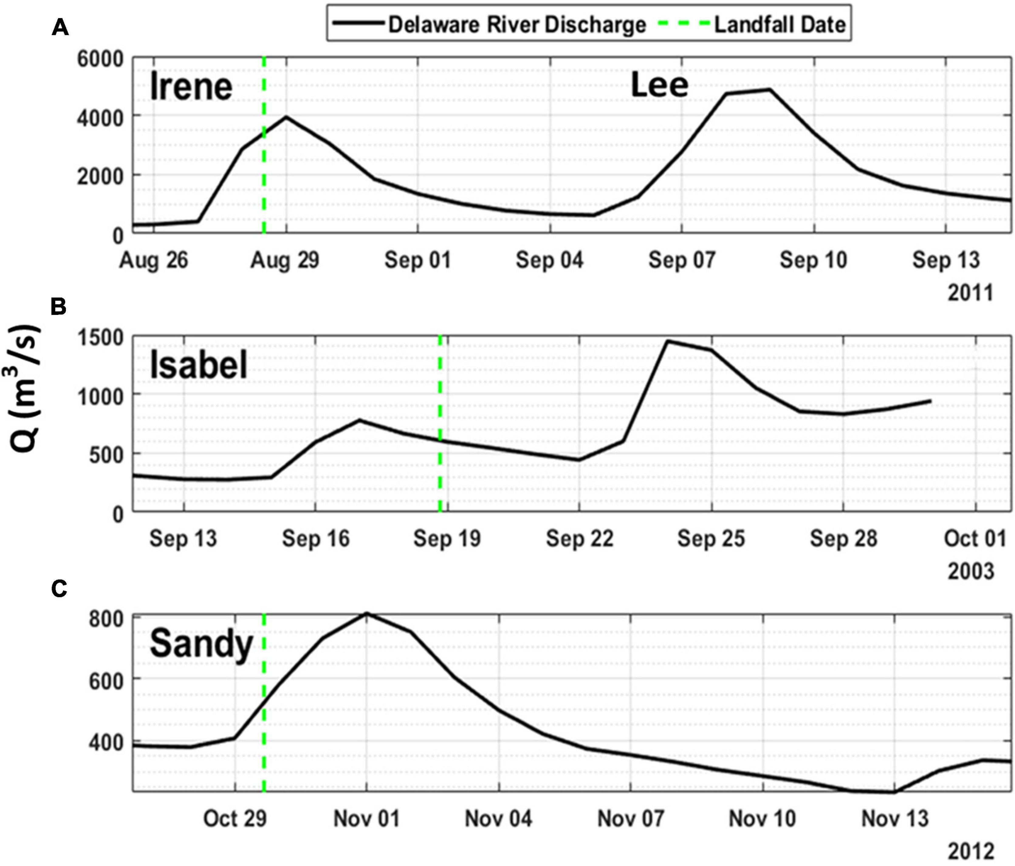
Figure 6. Delaware River discharge at Trenton (USGS 1463500, Q1 in Figure 1B) during historical extreme events: (A) Irene and Lee; (B) Isabel; and (C) Sandy.
To compare the non-linear terms produced by different forcings during Irene (a compound flooding event), numerical experiments were conducted and are summarized in Table 1. Results from two model runs, TO run (driven by tides only) and TSR run (driven by tides, surface winds, and river flow), were processed to extract TSRI following the method described in section “TWL and Non-linear Interaction Decomposition.” To distinguish TSI and TRI from TSRI during Hurricane Irene, the TS run (driven by tides and surface winds) and the TR run (driven by tides and river flow) were designed to mimic the Irene event but the individual river flows and surface winds were removed; thus the non-linear interaction induced by TSI only and TRI only during Irene, as well as their effect on TSRI, could be estimated.
Furthermore, a series of sensitivity model runs were conducted to investigate the response of TSRI during Irene with river flows (TSR SensQ) corresponding to different recurrence intervals (ARIs), commonly known as return periods, and the impact of TSRI on TWLs. The surface wind field and open boundary of water levels were kept the same as those during Hurricane Irene in the TSR run.
Model Validation With Water Levels
To validate the storm surge model of DBE, model performance in simulating the TWL during extreme events was evaluated by comparing modeled water levels in the TSR run to observed data at the NOAA 10 tide gauges for three one-month-long periods that corresponded to four extreme events—Hurricane Irene and Tropical Storm Lee (August 20, 2011 to September 20, 2011), Hurricane Sandy (October 20, 2012 to November 20, 2012), and Hurricane Isabel (September 01, 2003 to September 30, 2003).
Model parameters, such as the bottom roughness and open-boundary sponge layer (radius and friction coefficient), were first calibrated based on Hurricane Irene and Tropical Storm Lee and then validated for Hurricanes Sandy and Isabel. Figure 7 shows the scatter-plot comparisons for simulated and observed water levels at the 10 tide gauges in the DBE for the three simulations periods. Overall, the model-predicted water levels match the observed data variation trend well and the model reproduces the tidal amplification toward upstream inside the DBE. However, the model tends to underpredict the TWL at some locations, such as at the PA station during Sandy and Isabel, and the SJS and CM stations, respectively, during the Irene and Lee events.
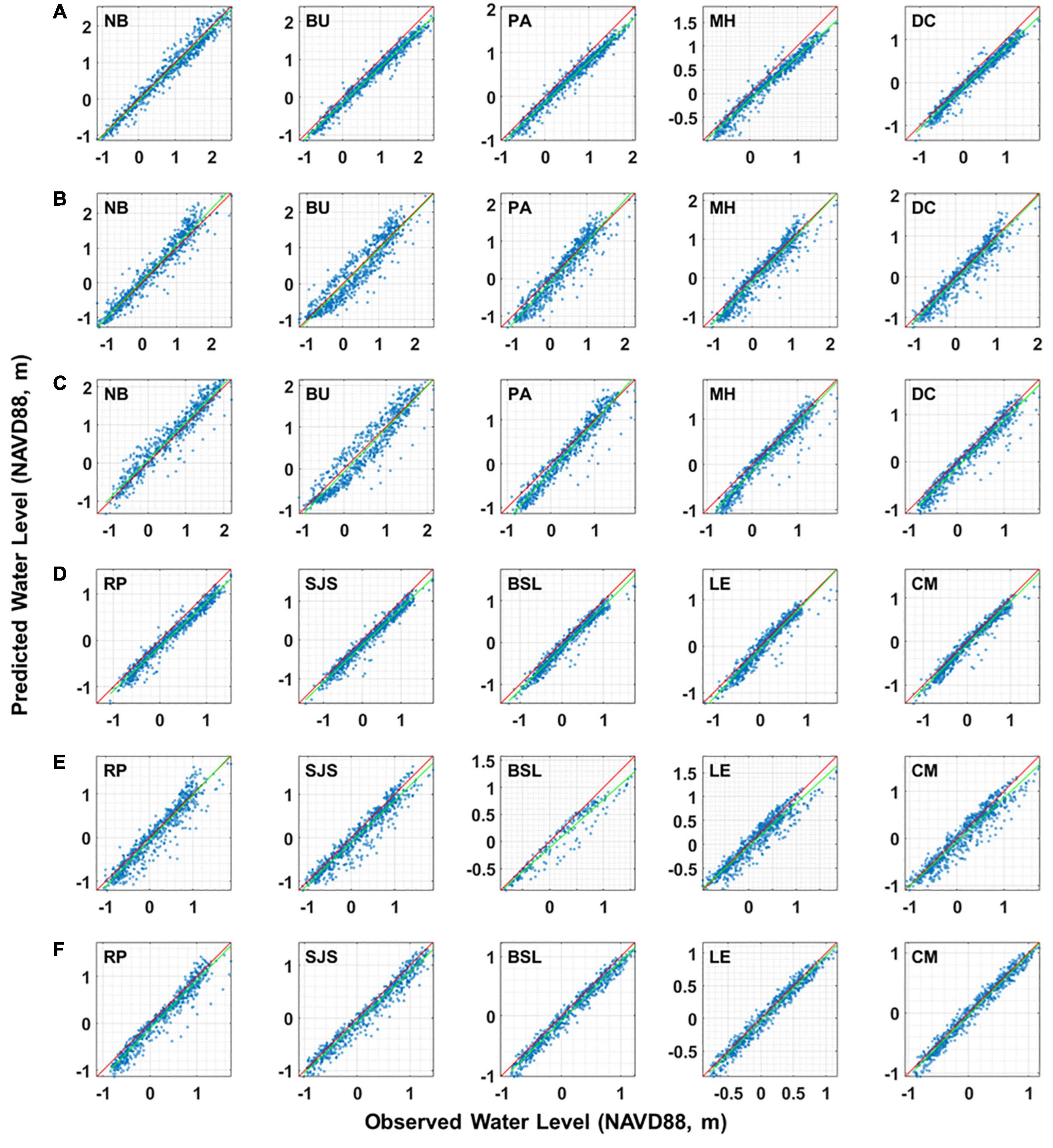
Figure 7. Scatter comparisons of simulated and observed water levels at 10 tidal stations during three simulation periods in the DBE; (A,D) Irene and Lee: August 20 to September 20, 2011; (B,E) Sandy: October 20 to November 20, 2012; (C,F) Isabel: September 01 to 30, 2003. The red line represents the 1-to–1 fit and the green line represents the linear correlation between model and data.
To quantify the model’s skill in simulating water level in the DBE, a set of model performance metrics were calculated. Specifically, the following four error statistical parameters were used.
The root-mean-square-error (RMSE) is defined as:
where, N is the number of observations, Mi is the measured value, and Pi is the model-predicted value.
The scatter index (SI) is the normalized RMSE with the average magnitude of measurements:
The bias (Bias) is defined as the mean difference between model predictions and the measurements:
The linear correlation coefficient (R) is a measure of the linear relationship between model predictions and the measurements:
The error statistics for the simulated water levels at all tide gauges are provided in Table 2. The RMSE varies within a range between 0.15 and 0.26 m with an increasing trend in the upstream, likely due to the effects of the complicated geometry of narrow and meandering channels. The SI values, which measure the normalized RMSE, vary from 0.22 in the estuarine mouth to 0.38 in the river mouth. The Bias values at all stations are within a range of −0.06 to −0.20 m, which also suggests the model is slightly underestimating water levels. The linear correlation coefficient R is 0.98 at all the stations except at the very upstream station Newbold (0.97) and the downstream station at Lewes (0.96), indicating the model predictions strongly correlate with field observations.
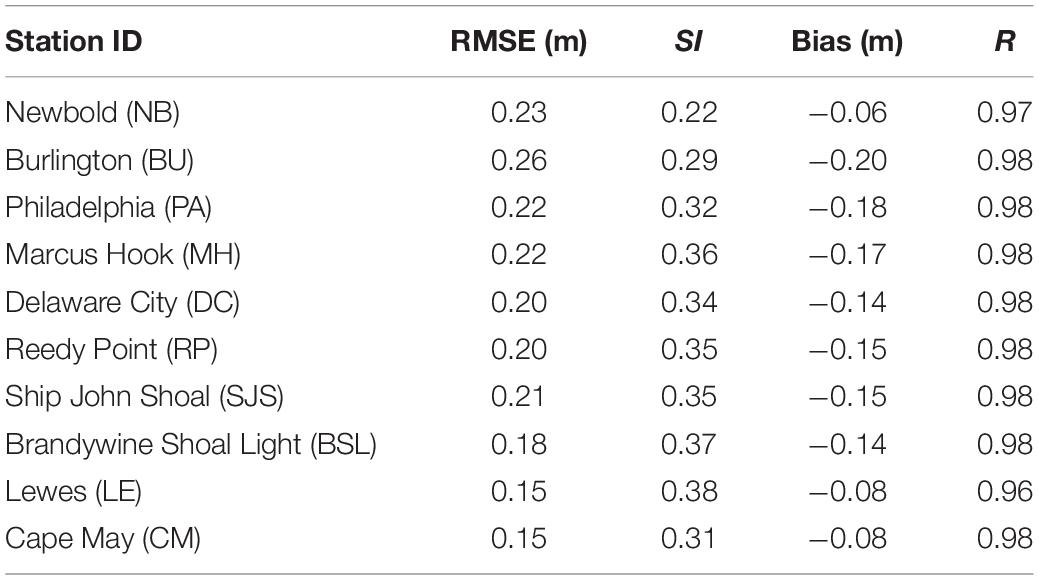
Table 2. Error statistics of water-level predictions in the DBE.
The simulated major tidal harmonic constant (M2) was also compared with observed data at ten tide gauges (Table 3). The maximum difference between simulated and observed M2 tidal constituent is −0.13 m at NB station, which is about 12.1% underprediction by the model. More accurate bathymetry and high model resolution may be required to improve the model accuracy in very upstream region of the estuary. Model predictions of M2 tide at the rest tide gauges matched the data reasonably well. Therefore, the overall performance of the model in simulating tidal elevation is considered satisfactory.
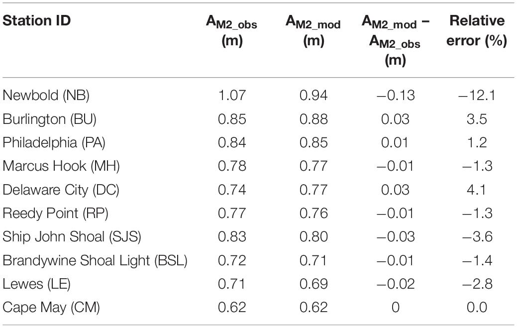
Table 3. Comparison of observed and modeled M2 tidal amplitude in the DBE.
Results and Discussion
Contribution of TSRI to TWL
Previous studies suggest that TSRI increases the uncertainty in TWL prediction (Doodson, 1956; Proudman, 1957; Rossiter, 1961; Johns et al., 1985; Arns et al., 2020). To understand the effects of TSRI on TWLs and coastal flooding in the DBE, TSRI was derived for the four extreme events.
Figure 8 shows the time series of the simulated TWL, astronomical tides, LFS, and TSRI—at the NB, PA, and LE stations, located at the upstream, upper bay, and lower bay, respectively. To better understand the effect of TSRI on TWL, the unmodulated total water level (UTWL), which is simply a linear superposition of tide and LFS, was also plotted in Figure 8. Comparison of the TWL and UTWL indicates that modulations from TSRI on TWL vary with locations and extreme events. During Hurricane Irene (Figure 8A)., TSRI was the product of tides interacting with river and storm surges in turn to manifest TWL at a tidal frequency. TSRI at the LE station, which is located in the downstream of DBE, is storm surge driven for four extreme events, indicating less effect on TWL because there was little difference between TWL and UTWL (Figure 8C). TSRI at the NB station is dominated by river flow, showing strong tidal signals (Figure 8A). TSRI at NB suppressed tidal variations by more than 50% of the tidal range. TSRI at PA is less river dominant and does not feature prolonged damping on tides (Figure 8B).
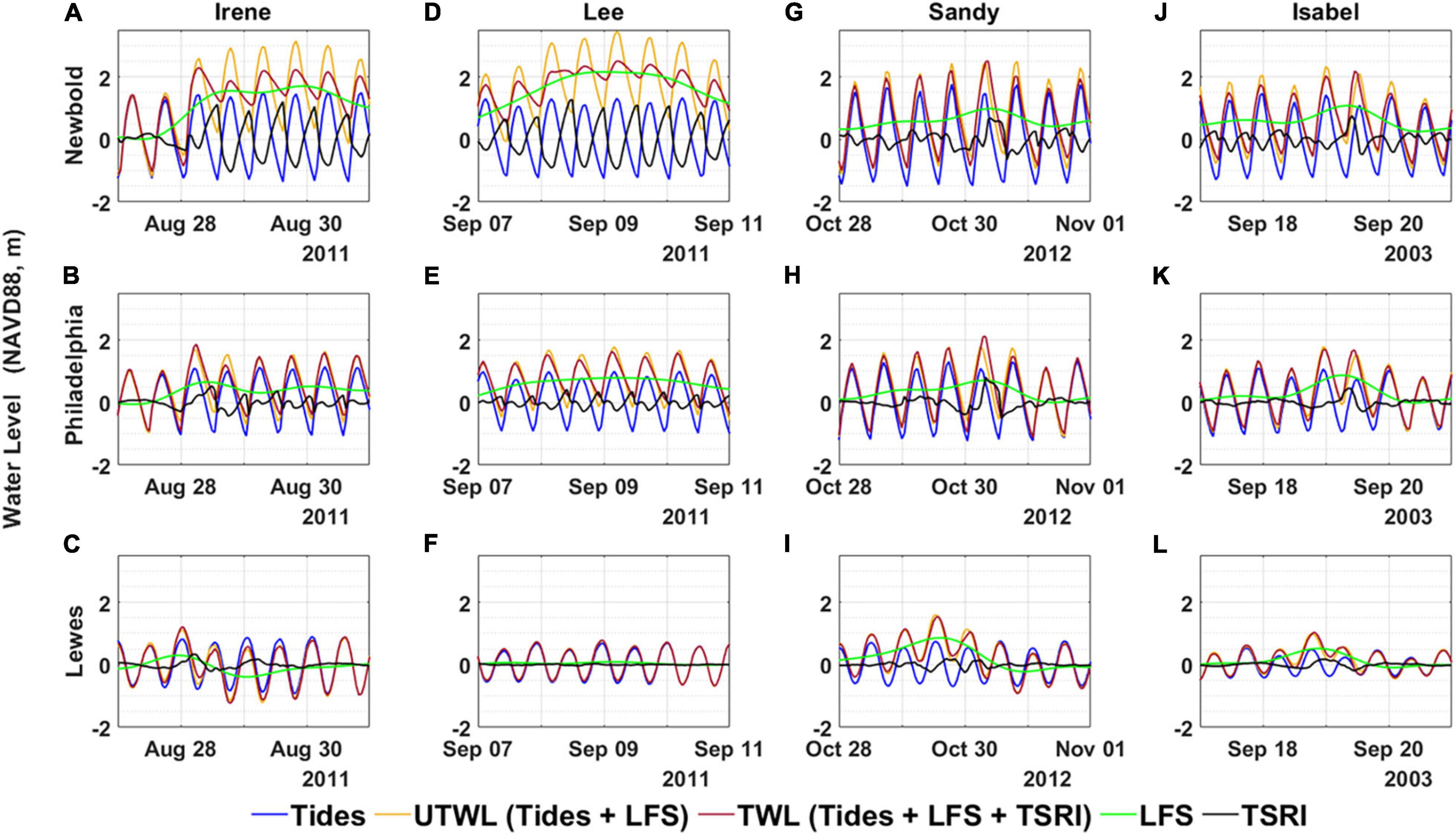
Figure 8. Modeled tides (blue), LFS (green), TSRI (black), TWL (dark red), and UTWL (tides + LFS, orange) during Irene (A–C), Lee (D–F), Sandy (G–I), and Isabel (J–L) at tidal gauges Newbold (NB), Philadelphia (PA), and Lewes (LE) (top to bottom).
During Tropical Storm Lee, which featured strong river flow and little storm surge, TWL at NB is significantly elevated up to 2.1 m by LFS, but the tidal range is much reduced (Figure 8D), similar to during Hurricane Irene. TSRI at NB had an amplitude (up to 1.2 m) similar to tides during peak river flow but in an opposite phase, resulting in the weakening of the tidal fluctuations. Strong TSRI lasted more than 4 days during high river flow, which demonstrated that TSRI was in a direct proportion to the river flow (Godin and Martinez, 1994; Sassi and Hoitink, 2013). Without the effect of TSRI, as shown in the UTWL, the tidal variations were maintained and the maximum UTWL was up to 1.0 m higher than the maximum TWL (Figure 8D). Downstream of NB, the magnitude of TSRI was greatly reduced to a level of 10 to 15% of TWL at PA (Figure 8E) and approached zero at LE (Figure 8F), because neither river flow nor storm surge affected TWL at the mouth of DBE during Tropical Storm Lee.
Hurricanes Sandy and Isabel featured strong storm surges, but had river flows smaller than those during Irene and Lee. TSRI from downstream (LE) to upstream (PA, NB) were mainly induced by the storm surges, and the peaks of TSRI increased from about 0.2 to 0.8 m as water depth became shallower (Figures 8G–L). Wind stress-induced surge magnitude is understood to be significantly greater at low water than at high water (Horsburgh and Wilson, 2007; Rego and Li, 2010; Zheng et al., 2020). The shallower the water depth, the stronger the tidal current magnitude, which resulted in stronger TSRI.
Unmodulated total water level shows both magnitude and phase differences from TWL at PA and NB during landfall of Sandy and Isabel (Figures 8G,H,J,K). Previous studies indicated that the effect of TSRI on surges is through magnitude modulation, and the effect on tides is through phase shift (Horsburgh and Wilson, 2007). The peak of TSRI occurred on falling tide during Sandy but on rising tide during Isabel, where TWL propagated faster than UTWL during Sandy but slower than UTWL during Isabel. In an idealized first-order modeling study, Horsburgh and Wilson (2007) discovered that that the peak TSRI with respect to high tide does not occur randomly but in clusters on the rising or falling tides, depending on the phase speed between TWL and tides. Therefor when tides lead the TWL (such as Isabel), the TSRI will peak halfway up the rising tide. On the other hand, when tides lag TWL (such as Sandy), TSRI will peak on the falling tide. The changes of phase speeds of surge and tide can be explained by the increase of bottom friction effect due to the reduced water depth (Wolf, 1981).
Contribution of TSRI to Tidal Modulation
Tides interact with different physical processes and generate non-linear interactions at tidal frequencies, which affect the tidal variations of TWL. This process is seen as tidal modulation by TSRI on TWL. Because TSRI varies with tidal frequency, it is helpful to conduct frequency analysis of TSRI to understand how different tidal bands interact with LFS. By decomposing the TSRI based on the tidal frequency (mainly focusing on diurnal D1, semidiurnal D2, and quarter-diurnal D4 bands), the effects of tidal modulation by TSRI on TWL were assessed and quantified during the four extreme events. This section describes how non-stationary tidal analysis—Complex Demodulation as described in section “TWL and Non-linear Interaction Decomposition”—was applied to the time series of TSRI to calculate the time-varying amplitude and phase at different tidal frequencies. The reconstructed time series of TSRI at the D1, D2, and D4 bands at the upstream NB station are presented in Figure 9.
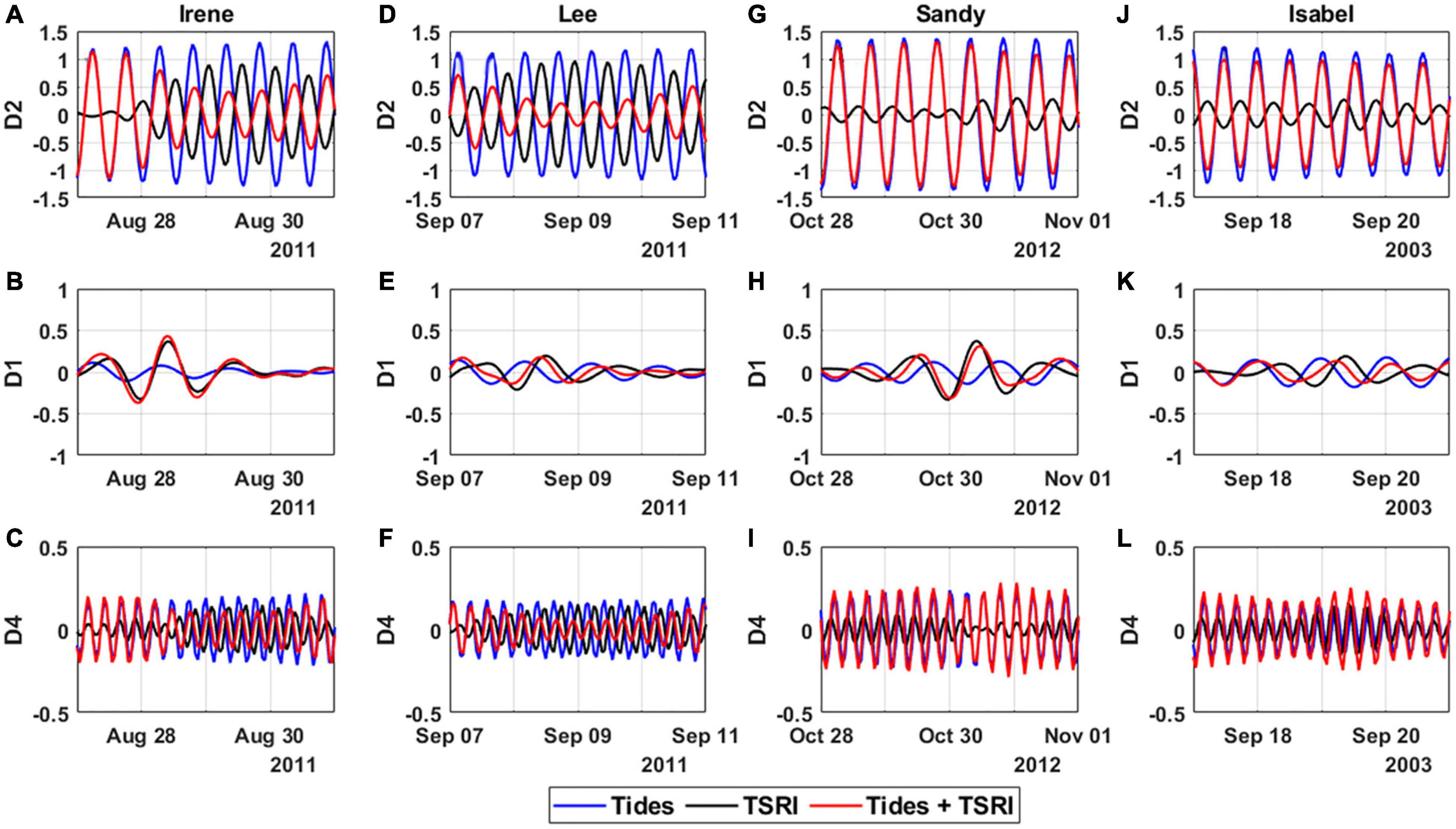
Figure 9. Time series of predicted tides (blue), TSRI (black), and tides plus TSRI (red) for the D2, D1, and D4 bands (top to bottom) during Irene (A–C), Lee (D–F), Sandy (G–I), and Isabel (J–L) at the NB station.
The amplitude of the D2 component of TSRI during strong river flow (Irene and Tropical Storm Lee) can reach up to 1 m, which is comparable to semidiurnal tides, and the time series is out of phase with a 6-h lag relative to tides (Figures 9A,D). Therefore, the tidal modulation by TSRI on TWL at the D2 band has a damping effect. The amplitude of tidal variations of TWL (red line in Figures 9A,D) at the D2 band is reduced by more than 50% of the amplitude of semidiurnal tides (blue line in Figures 9A,D). The contribution of TSRI to tidal modulation at the D2 band during Sandy and Isabel was insignificant, as shown in Figures 9G,J. The amplitude of the D1 component of TSRI can reach up to 0.4 m during strong storm surge events induced by Sandy and Irene, about 2 times greater than diurnal tides (Figures 9B,H). The tidal modulation by TSRI on TWL at the D1 band enhanced the diurnal tides in a dominant way. The amplitude of the D4 component of TSRI is less significant in NB station for all the four extreme events (Figures 9C,F,I,L). However, the phase of TSRI at the D4 band works against the tides when the river flow is strong, such as during Irene and Lee (Figures 9C,F).
The peak amplitudes of TSRI at the D2, D1, and D4 bands and the corresponding amplitudes for tides, as well as the sum of the two, are plotted in Figure 10 for 10 tidal gauges, in order from upstream to downstream in the DBE. During Hurricane Irene and Tropical Storm Lee, it is clear that river flow mainly interacts with tides at the D2 band and results in TSRI damping semidiurnal tides until the river flow impact ceases at MH station (Figures 10A,D). Therefore, the higher the river flow, the greater the tidal modulation of damping on semidiurnal tides by TSRI, and the smaller the tidal variations of TWL at the D2 band. During Irene and Sandy, storm surges mainly interacted with diurnal tides, and the tidal modulation by TSRI on TWL at the D1 band was amplified. The tidal variations of TWL at the D1 band were enhanced by peak TSRI during Irene and Sandy, resulting in strong storm surges larger than diurnal tides (Figures 10B,H). High-frequency TSRI at the D4 band generally enhances tides except at the NB station during high river flow events (e.g., Irene and Lee), and the magnitude is overall not significant (Figures 10C,F,I,L).
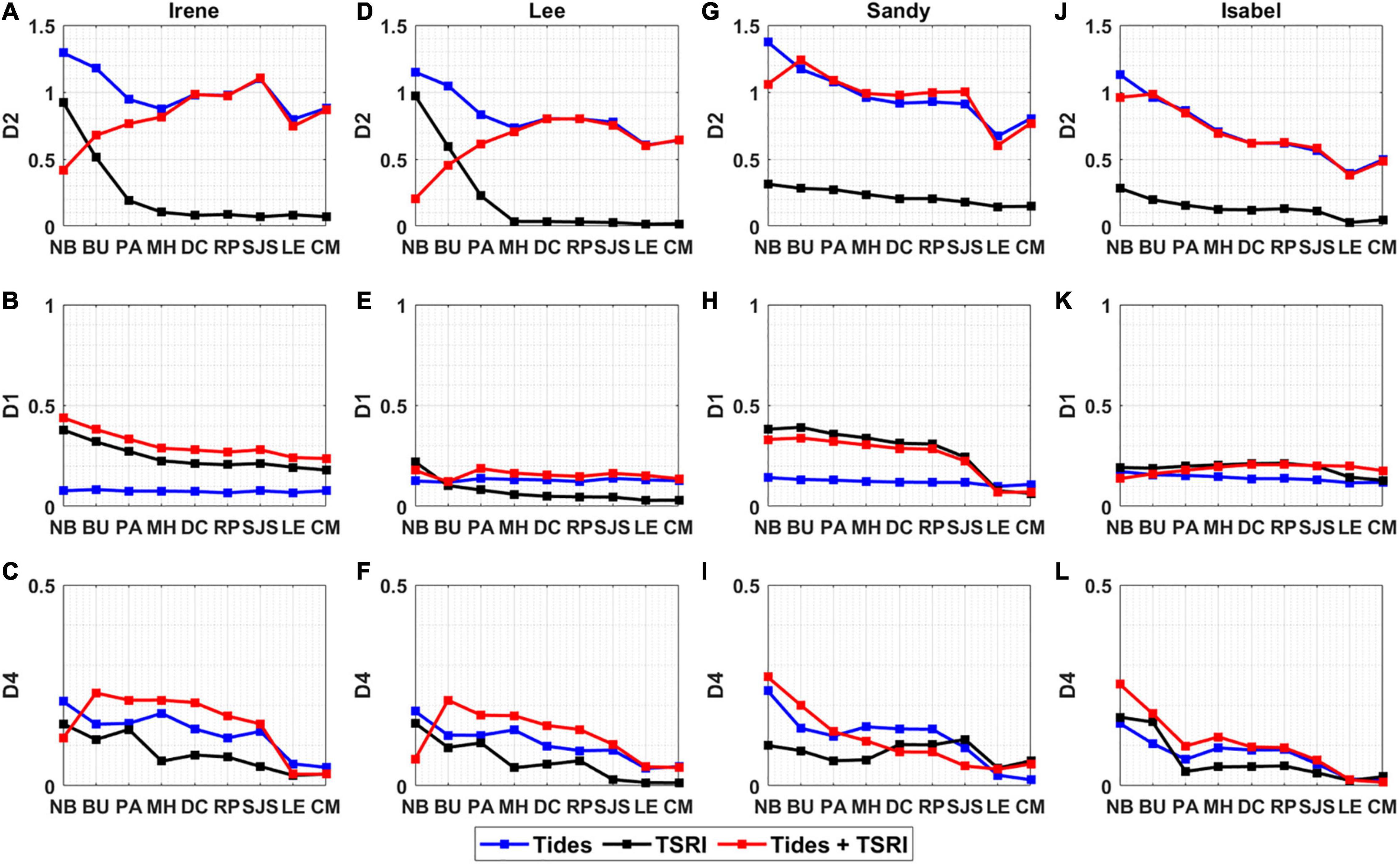
Figure 10. Predicted peak amplitudes of TSRI (black) and corresponding amplitudes of tides (blue), the sum of tides and TSRI (red) at the D2, D1, and D4 bands (top to bottom) at 10 tidal gauges during Irene (A–C), Lee (D–F), Sandy (G–I), and Isabel (J–L). Note: The vertical scales for the D2, D1, and D4 bands are not the same.
From upstream to downstream, the tidal modulations by TSRI on TWL at the D2, D1, and D4 bands all show a decreasing trend as water depth increases. The TSRI at the D2 band shows greater variations and larger magnitudes than those at the D1 band when the impact of river flow is significant. Therefore, the tidal modulation on TWL by TSRI is dominated by the river-induced damping effect during high flow events. Storm surge-induced amplification becomes the dominant effect when river flow is low.
Effects of River Flow and Storm Surge on Compound Flooding
For Hurricane Irene, which featured high river flow and large storm surge, the effects of river-induced damping by TRI and storm surge-induced amplification by TSI on TWL co-exist during compound flooding (e.g., Figures 10A,B). As indicated in the previous section, TRI mainly damps on semidiurnal tides (D2 band) and TSI enhances diurnal tides (D1 band). To better understand the combined effect of TRI and TSI on the TWL, numerical experiments (TR run and TS run) were conducted to extract TRI and TSI components from TSRI.
The spatial distributions of the peak magnitude of TRI, TSI, and TSRI inside the DBE during Hurricane Irene were compared (Figure 11) and further evaluated along a longitudinal transect. The DBE can be divided into three zones based on the pattern of TSRI: the river zone where TSRI is dominated by TRI in the upstream of the BU station and shows patterns similar to those in Figures 11A,C; the surge zone where TSRI is dominated by TSI downstream of the MH station and exhibits patterns similar to those in Figures 11B,C; and the transition zone where TSRI is influenced by both river flow (TRI) and storm surge (TSI) between the BU and MH stations (Figure 11C). Hoitink and Jay (2016) proposed the definition of boundary between tidal river and estuary using the point of reversal of lowest low waters from spring to neap (typically AMsf=AS2). It was found AMsf=AS2 ≈ 0.13m at the PA station where TS is delimiting but TR becomes dominant. The transition zone classification based on TSRI distribution also indicates the estuary-tidal river boundary.
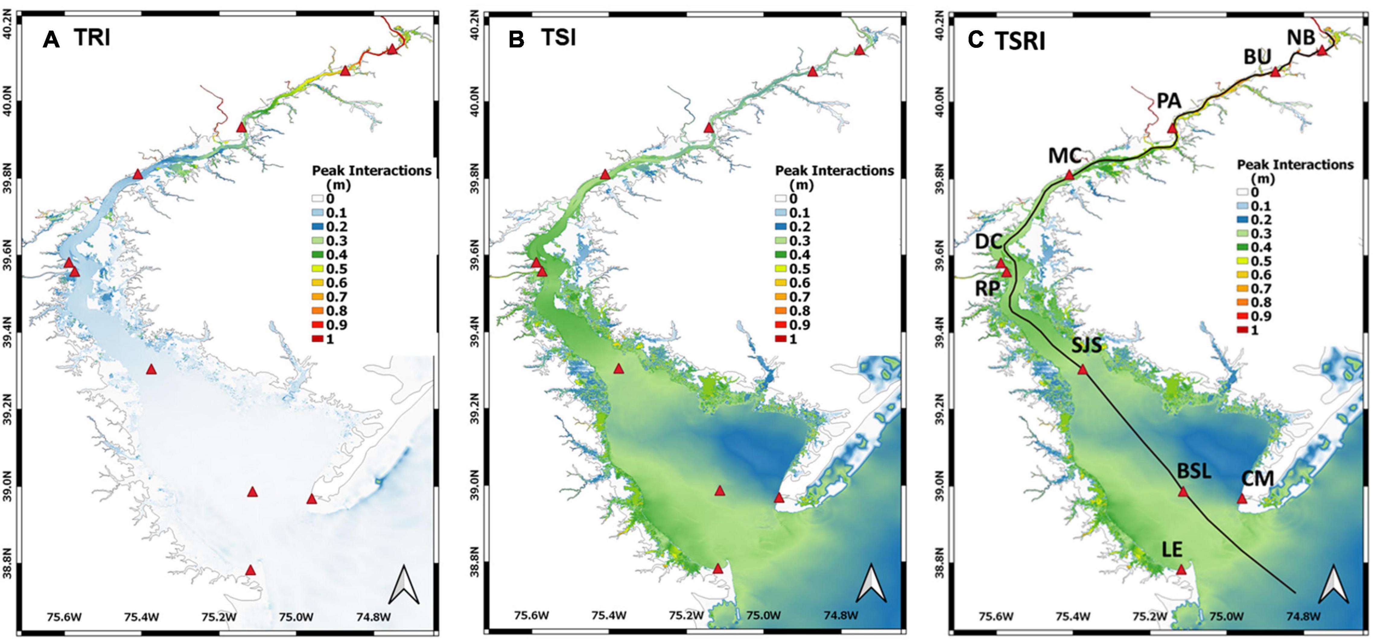
Figure 11. Spatial variations on peak values of (A) TRI, (B) TSI, and (C) TSRI during Hurricane Irene in the DBE. Tide gauges are labeled as red triangles.
To assess the level of impact of TRI, TSI, and TSRI on TWL, the modulation ratio is used, which is defined as:
where, UTWL = Tide + LFS at the same timestep of TWLmax. Based on the definition of TWL (Figure 4), Eq. (8) can be further written as:
The modulation ratio represents the modulation of non-linear interactions on TWL in terms of magnitude and phase change. Figure 12 shows that when only tide and river flow are considered (TR run, orange line), the TRI damps TWL by up to 40% in the upstream and the damping effect gradually reduces to zero around MH. In TS run (blue line), the TSI enhances TWL by 5–15% in the whole domain, but the effect on the TWL is smaller than the effect of river flow (Figure 12A). In the TSR run, a transition point of TSRI is shown around 230 km upstream between the PA and BU stations. At the very upstream, TSRI is damping TWL up to 40%, while downstream of the tipping points TSRI is enhancing TWL by 10–15% (Figure 12B).
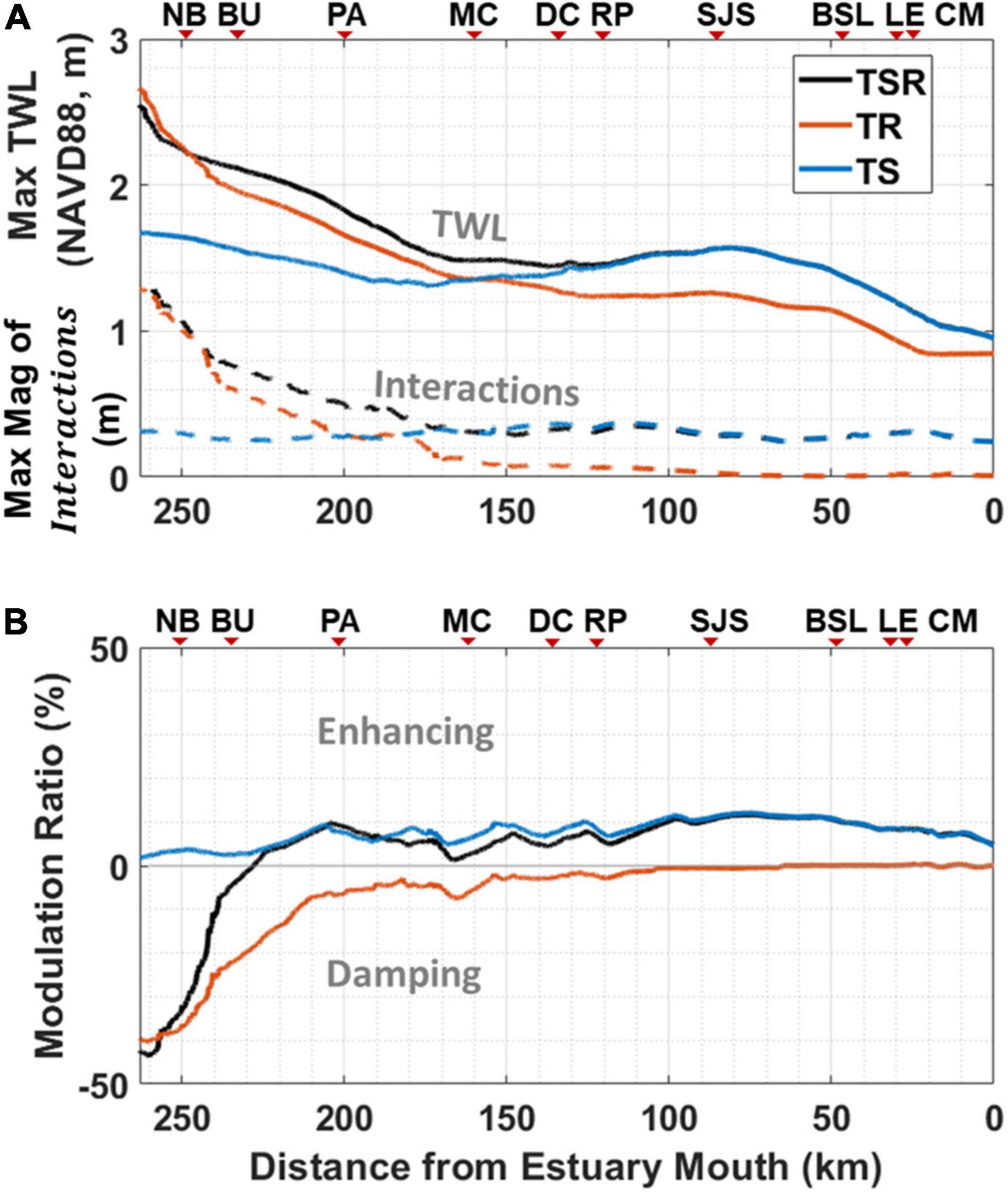
Figure 12. Along estuary variations in the TSR run (black), TR run (red), and TS run (blue) of (A) peak values of TWL and peak magnitude of non-linear interactions, (B) modulation ratio by non-linear interactions on TWL.
The frequency analysis in section “Contribution of TSRI to Tidal Modulation” details the variations in TSRI at different tidal frequencies (Figure 9), and the modulation ratio evaluates the impacts of non-linear interactions on TWL under different forcing mechanisms (Figure 12). To further quantify the relative contributions of the D2, D1, and high-frequency (D4+D6+D8) tidal bands to the total variance of TRI, TSI, and TSRI, the SSA method (described in section “TWL and Non-linear Interaction Decomposition”) was applied at 10 tide gauges. Figure 13A shows that TRI is contributed by D2 and high-frequency bands only and the contribution from the D1 band is zero. The D2 band contributes 70 to 90% of the total variability of TRI at the NB and BU stations, while the high-frequency band contributes more than 50% of the total variability of TRI at the PA and MH stations, which indicates the shallow water effect becomes dominant in this area. The lower contribution of the high-frequency band to the total variability of TRI at upstream locations (NB and BU) with respect to D2 was attributed to a faster damping of the higher harmonics by river flow. Further downstream of MH, TRI is less than 0.2 m and becomes negligible. However, for the TS run, TSI is predominantly contributed by the D1 band in a range of 50 to 80% in the entire DBE (Figure 13B). In the TSR run, which considered the combined forcing of tide, river flow, and storm surge, the contribution of TSRI followed a three-zone pattern (Figure 13C), as described in section “Effects of River Flow and Storm Surge on Compound Flooding.” The D2 and D1 bands contribute the most to TSRI in the upstream and downstream of the estuary, respectively. In the transition zone around PA, the high-frequency band contributes up to 60% of the total variance of TSRI (Figure 13C). The contributions to the total variance of TRI, TSI, and TSRI from the identified D2, D1, high-frequency (D4+D6+D8) bands at 10 tidal gauges are summarized in Table 4.
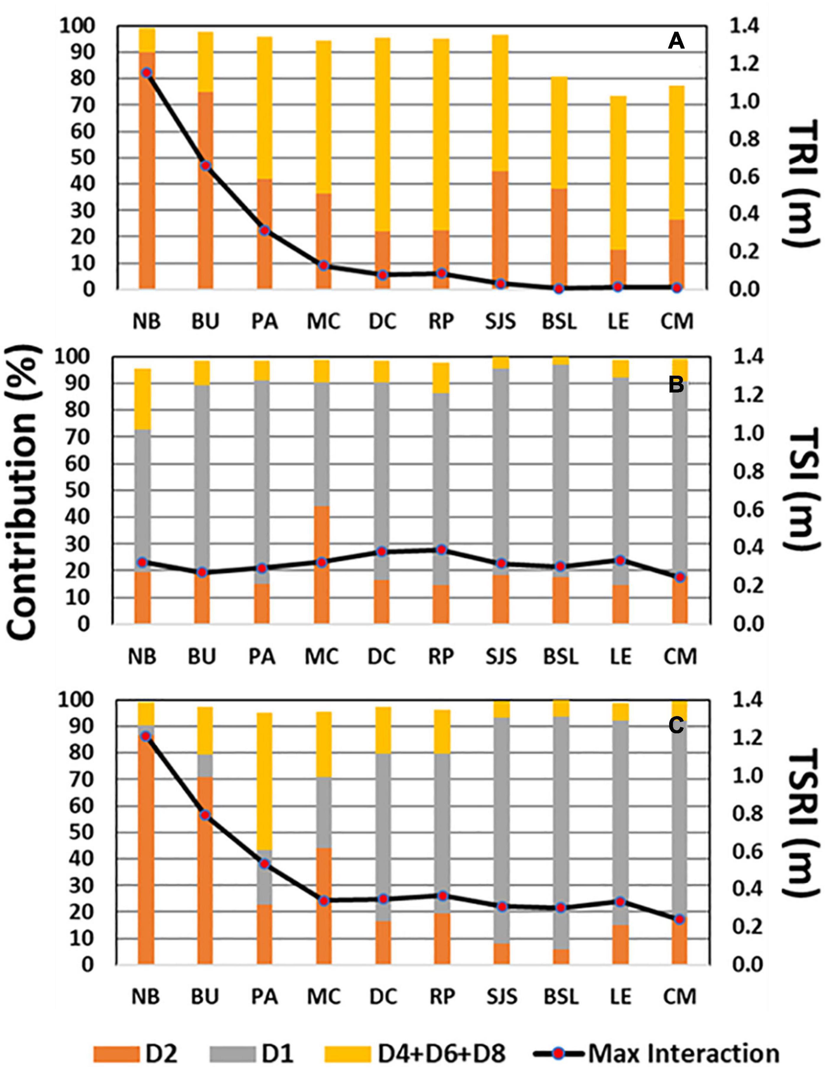
Figure 13. Peak values of (A) TRI, (B) TSI, (C) TSRI (black lines), and the percentage of relative contributions from different tidal bands [D2 – semi-diurnal band (red); D1 – diurnal band (gray); D4+D6+D8 – high-frequency (orange)] to the total variance of corresponding non-linear interactions at 10 tidal gauges.
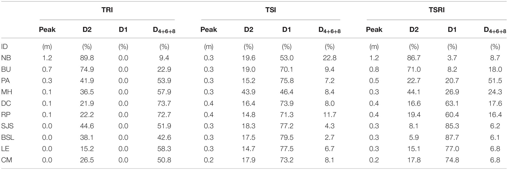
Table 4. Relative contributions (%) of the D2, D1, and high-frequency (D4+D6+D8) bands to the total variance of TRI, TSI, and TSRI at 10 tidal gauges.
Sensitivity of River Flow on Compound Flooding
As discussed in previous sections, TSRI is proportional to river flow and has a damping effect on tidal amplitude, which is caused by the bottom friction effect via dissipating tidal energy (Godin, 1999; Horrevoets et al., 2004). However, the relationship between tidal damping and river flow rate can be linear or non-linear in different estuaries. Tidal damping by TSRI is dominated by the river flow in the upstream of tidal estuaries (Godin and Martinez, 1994). Theoretical analysis suggested a linear relationship between tidal damping modulus and river flow in the Columbia River estuary (Kukulka and Jay, 2003). However, Guo et al. (2015) found non-linear tidal decay of principal tides and the modulation of M4 tide with increasing river flow in the Yangtze River estuary. To better understand the relationship between the damping effect and river flow in the DBE, a sensitivity analysis was conducted to evaluate the damping effect of TSRI on TWL in the DBE under different river flow conditions.
To determine the river flow range corresponding to a flood return period, a rating curve of flood frequency for the Delaware River was developed using USGS stream gauge data at Trenton. Figure 14 indicates that Irene is equivalent to a 5 year flood event while Tropical Storm Lee corresponds to a 10 year flood event. Sensitivity model runs were carried out with stream flows corresponding to flood return periods of 2, 5, 10, 25, 50, 100, and 500 years. The hydrograph shape of the Irene event was used to construct the river flow input by multiplying a ratio to match the peak design flows to simulate Irene-like river flood events. Tide and wind field were kept the same as those used in Hurricane Irene.
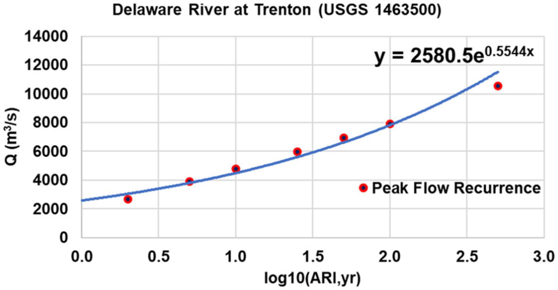
Figure 14. Flood frequency chart of the Delaware River based on USGS data.
The variations of the peak TWL and peak magnitude of TSRI under different river flows from upstream to downstream and the corresponding modulation ratios by TSRI on TWL are shown in Figure 15. The magnitude of TSRI and TWL from upstream to the MH station is affected by river flow changes; the maximum variations of TSRI and TWL in the upstream were approximately in the ranges of 1–2 m and 2.2–5.5 m, respectively (Figure 15A). The larger increase in TWL compared to TSRI is due to the increase in LFS induced by river flow. In general, downstream of station MH, the variation of river flow has little influence on TWL and TSRI, and modulation ratio. However, approximately between stations BU and MH, the effects of river flow rates on TWL, TSRI, and modulation ratio become evident, with TWL and TSRI increasing toward the upstream as a function of flow rate (Figure 15A) and the modulation ratio transitioning from enhancing to damping (Figure 15B). It is also observed that the transition location of the modulation ratio shifts downstream as river flow increases (Figure 15B). It is interesting to see the modulation ratio reaching a minimum (or maximum damping) in the upstream zone and the minimum inversely proportional to the flow rate and ARI (Figure 15B). For example, the respective minimums of the modulation ratio corresponding to ARIs of 5 yr, 25 yr, and 500 yr are approximately −43, −40, and −33%. The presence of the minimum of modulation ratio can be explained by its definition in Eq. (9), which is non-linear interactions divided by TWL. In the transition zone, the relative increase in the damping effect from non-linear interactions is greater than the increase in TWL. However, toward the upstream, TWL increases significantly with a greater rate and results in a reduction in the magnitude of the modulation ratio, and consequently the maximum damping.
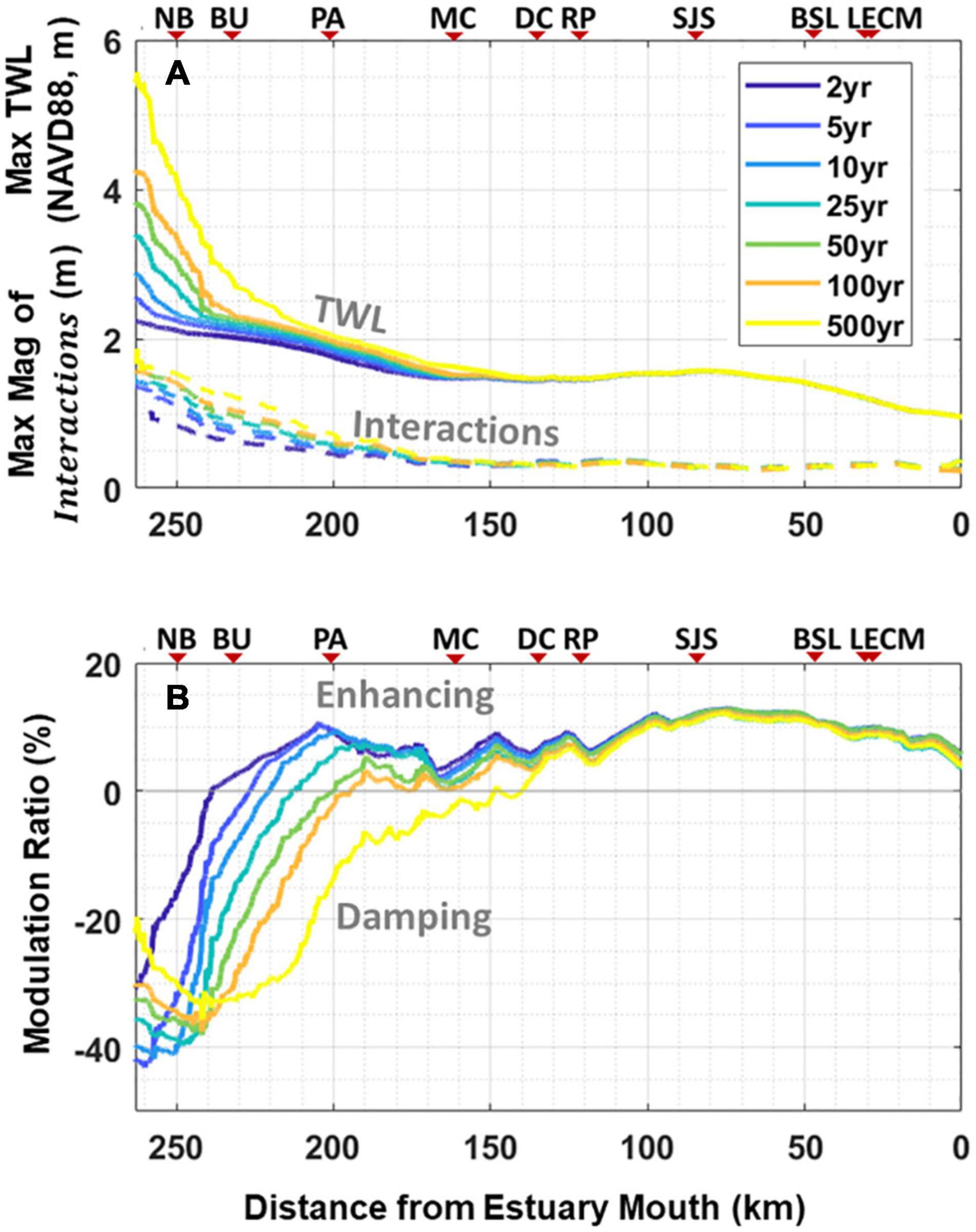
Figure 15. Along-estuary variations of (A) peak magnitude of non-linear interactions and peak TWL corresponding to a range of return periods (2–500 years ARI) from the Delaware River; (B) modulation ratio by TSRI on TWL.
Summary and Conclusion
In this study, a 3-D, high-resolution storm surge model was developed to evaluate the non-linear interactions between tidal and non-tidal components of TWLs in the DBE during hurricane events. In particular, focused analysis was conducted to understand the effect of non-linear interactions on coastal compound flooding induced by the co-occurrence of river floods and coastal storm surges. Specifically, storm surge and non-linear interactions induced by historical extreme weather events—Hurricanes Isabel (2003), Irene (2011), Tropical Storm Lee (2011), and Sandy (2012) – were simulated and analyzed.
The model was validated with observed water levels at 10 tide gauges that span the entire DBE. Simulated water levels were decomposed to astronomical tides, LFSs, and non-linear interactions. The effects of non-linear interactions on the TWL were further analyzed using a wavelet approach and a spectral analysis method. TRI and TSI were derived using numerical experiments driven by the corresponding forcing only. The DBE can be divided into three zones: the river-dominated (upstream of the BU station), the storm surge-dominated (downstream of station MH), and the transition zone in between. Analysis results indicate that TRI tends to damp tidal amplitude on the D2 band, by up to 40% of the TWL, in the upstream river-dominated zone, caused by the bottom friction effect via dissipating tidal energy (Godin, 1999; Horrevoets et al., 2004). However, TSI amplifies tides on the D1 band by 10 to 15% of TWL in the entire estuary.
The effect of TSRI on TWL was more noticeable during compound flooding events such as Hurricane Irene. TSRIs in the river and surge zones are dominated by TRI and TSI to dampen and enhance TWL, respectively. TSRI in the transition zone is jointly contributed to by TRI and TSI, which yields a tipping point of separating the damping and enhancing effects in the estuary. Sensitivity analysis indicated that the tipping point of TSRI damping and enhancing effects shifts downstream as river flow ARI increases.
Data Availability Statement
The raw data supporting the conclusions of this article will be made available by the authors, without undue reservation.
Author Contributions
ZY, ZX, and TW contributed to conception and design of the study. ZX, ZY, and TW contributed to the methodology. NS and MW contributed to the river flow analysis. ZX performed the simulations, visualization, and results analysis. DJ provided project administration. ZX and ZY wrote the first draft of the manuscript. All authors contributed to manuscript review, revision, and approved the submitted version.
Funding
This work was supported by the MultiSector Dynamics, Earth System Model Development and Regional and Global Modeling and Analysis program areas of the United States Department of Energy, Office of Science, Office of Biological and Environmental Research as part of the multi-program, collaborative Integrated Coastal Modeling (ICoM) project. All model simulations were performed using resources available through Research Computing at Pacific Northwest National Laboratory.
Conflict of Interest
The authors declare that the research was conducted in the absence of any commercial or financial relationships that could be construed as a potential conflict of interest.
Publisher’s Note
All claims expressed in this article are solely those of the authors and do not necessarily represent those of their affiliated organizations, or those of the publisher, the editors and the reviewers. Any product that may be evaluated in this article, or claim that may be made by its manufacturer, is not guaranteed or endorsed by the publisher.
Acknowledgments
The authors thank Dr. Isabel Jalón-Rojas for providing the MATLAB script of the complex demodulation method.
Footnotes
References
Amante, C., and Eakins, B. W. (2009). ETOP01 1 Arc-Minute Global Relief Model: Procedures, Data Sources and Analysis, OAA Technical Memorandum NESDIS, NGDC-24. 19.
Aristizabal, M., and Chant, R. (2013). A numerical study of salt fluxes in delaware bay estuary. J. Phys. Oceanogr. 43, 1572–1588. doi: 10.1175/Jpo-D-12-0124.1
Arns, A., Wahl, T., Wolff, C., Vafeidis, A. T., Haigh, I. D., Woodworth, P., et al. (2020). Non-linear interaction modulates global extreme sea levels, coastal flood exposure, and impacts. Nat. Commun. 11:1918. doi: 10.1038/s41467-020-15752-5
Bevacqua, E., Maraun, D., Vousdoukas, M. I., Voukouvalas, E., Vrac, M., Mentaschi, L., et al. (2019). Higher probability of compound flooding from precipitation and storm surge in Europe under anthropogenic climate change. Sci. Adv. 5:eaaw5531. doi: 10.1126/sciadv.aaw5531
Bloomfield, P. (2004). Fourier analysis of Time Series: An Introduction. Wiley Series in Probability and Statistics. Hoboken, NJ: John Wiley.
Chen, C., Gao, G., Zhang, Y., Beardsley, R. C., Lai, Z., Qi, J., et al. (2016). Circulation in the Arctic Ocean: results from a high-resolution coupled ice-sea nested Global-FVCOM and Arctic-FVCOM system. Prog. Oceanogr. 141, 60–80. doi: 10.1016/j.pocean.2015.12.002
Chen, C. S., Lai, Z. G., Beardsley, R. C., Sasaki, J., Lin, J., Lin, H. C., et al. (2014). The March 11, 2011 Tahoku M9.0 earthquake-induced tsunami and coastal inundation along the Japanese coast: a model assessment. Prog. Oceanogr. 123, 84–104. doi: 10.1016/j.pocean.2014.01.002
Chen, C. S., Liu, H. D., and Beardsley, R. C. (2003). An unstructured grid, finite-volume, three-dimensional, primitive equations ocean model: application to coastal ocean and estuaries. J. Atmos. Ocean. Technol. 20, 159–186. doi: 10.1175/1520-0426(2003)020<0159:augfvt>2.0.co;2
Dean, R. G. (1966). “Tides and harmonic analysis,” in Estuary and Coastline Hydrodynamics, ed. A. T. Ippen (New York, NY: MHGraw-Hill), 197–229.
Dinapoli, M. G., Simionato, C. G., and Moreira, D. (2021). Nonlinear interaction between the tide and the storm surge with the current due to the river flow in the rio de la Plata. Estuaries Coasts 44, 939–959. doi: 10.1007/s12237-020-00844-8
Doodson, A. T. (1956). Tides and storm surges in a long uniform gulf. Proc. R. Soc. Lon. Series A Math. Phys. Sci. 237, 325–343. doi: 10.1098/rspa.1956.0180
Dronkers, J. J. (1964). Tidal Computations in Rivers and Coastal Waters. Amsterdam: North-Holland Publishing Company.
Flinchem, E. P., and Jay, D. A. (2000). An introduction to wavelet transform tidal analysis methods. Estuarine Coastal Shelf Sci. 51, 177–200. doi: 10.1006/ecss.2000.0586
Gasquet, H., and Wootton, A. J. (1997). Variable-frequency complex demodulation technique for extracting amplitude and phase information. Rev. Sci. Inst. 68, 1111–1114. doi: 10.1063/1.1147748
Godin, G. (1999). The propagation of tides up rivers with special considerations on the upper saint lawrence river. Estuarine Coastal Shelf Sci. 48, 307–324. doi: 10.1006/ecss.1998.0422
Godin, G., and Martinez, A. (1994). Numerical experiments to investigate the effects of quadratic friction on the propagation of tides in a channel. Continental Shelf Res. 14, 723–748. doi: 10.1016/0278-4343(94)90070-1
Guo, L., van der Wegen, M., Jay, D. A., Matte, P., Wang, Z. B., Roelvink, D., et al. (2015). River-tide dynamics: exploration of nonstationary and nonlinear tidal behavior in the Yangtze River estuary. J. Geophys. Res. Oceans 120, 3499–3521. doi: 10.1002/2014JC010491
Hoitink, A. J. F., and Jay, D. A. (2016). Tidal river dynamics: implications for deltas. Rev. Geophys. 54, 240–272. doi: 10.1002/2015rg000507
Horrevoets, A. C., Savenije, H. H. G., Schuurman, J. N., and Graas, S. (2004). The influence of river discharge on tidal damping in alluvial estuaries. J. Hydrol. 294, 213–228. doi: 10.1016/j.jhydrol.2004.02.012
Horsburgh, K. J., and Wilson, C. (2007). Tide-surge interaction and its role in the distribution of surge residuals in the North Sea. J. Geophys. Res. Oceans 112(C8):4033. doi: 10.1029/2006JC004033
Hsiao, S. C., Chen, H., Chen, W. B., Chang, C. H., and Lin, L. Y. (2019). Quantifying the contribution of nonlinear interactions to storm tide simulations during a super typhoon event. Ocean Eng. 194:106661. doi: 10.1016/j.oceaneng.2019.106661
Idier, D., Bertin, X., Thompson, P., et al. (2019). Interactions between mean sea level, tide, surge, waves and flooding: mechanisms and contributions to sea level variations at the coast. Surv. Geophys. 40, 1603–1630. doi: 10.1007/s10712-019-09549-5
Idier, D., Dumas, F., and Muller, H. (2012). Tide–surge interaction in the English channel. Nat. Hazard Earth Sys. 12, 3709–3718. doi: 10.5194/nhess-12-3709-2012
Jalón-Rojas, I., Schmidt, S., and Sottolichio, A. (2016). Evaluation of spectral methods for high-frequency multiannual time series in coastal transitional waters: advantages of combined analyses. Limnol. Oceanogr. Methods 14, 381–396. doi: 10.1002/lom3.10097
Jalón-Rojas, I., Schmidt, S., and Sottolichio, A. (2017). Comparison of environmental forcings affecting suspended sediments variability in two macrotidal, highly turbid estuaries. Estuar. Coast. Shelf Sci. 198, 529–541. doi: 10.1016/j.ecss.2017.02.017
Jalón-Rojas, I., Sottolichio, A., Hanquiez, V., Fort, A., and Schmidt, S. (2018). To what extent multidecadal changes in morphology and fluvial discharge impact tide in a convergent (Turbid) Tidal River. J. Geophys. Res. Oceans 123, 3241–3258. doi: 10.1002/2017jc013466
Jay, D. A., and Flinchem, E. P. (1997). Interaction of fluctuating river flow with a barotropic tide: a demonstration of wavelet tidal analysis methods. J. Geophys. Res. 102, 5705–5720. doi: 10.1029/96jc00496
Johns, B., Rao, A. D., Dubinsky, Z., Sinha, P. C., and Lighthill, M. J. (1985). Numerical modelling of tide-surge interaction in the Bay of Bengal. Philos. Trans. Royal Soc. Lond. Series A Math. Phys. Sci. 313, 507–535. doi: 10.1098/rsta.1985.0002
Keers, J. F. (1968). An empirical investigation of interaction between storm surge and astronomical tide on the east coast of Great Britain. Dtsch. Hydrogr. Z. 21, 118–125. doi: 10.1007/bf02235726
Kukulka, T., and Jay, D. A. (2003). Impacts of Columbia River discharge on salmonid habitat: 1. A non-stationary fluvial tide model. J. Geophys. Res. 108(C9):3293. doi: 10.1029/2002JC001382
Landsea, C. W., and Franklin, J. L. (2013). Atlantic hurricane database uncertainty and presentation of a new database format. Mon. Wea. Rev. 141, 3576–3592. doi: 10.1175/mwr-d-12-00254.1
Lanzoni, S., and Seminara, G. (1998). On tide propagation in convergent estuaries. J. Geophys. Res.Oceans 103(C13), 30793–30812. doi: 10.1029/1998jc900015
Li, M., Zhang, F., Barnes, S., and Wang, X. (2020). Assessing storm surge impacts on coastal inundation due to climate change: case studies of Baltimore and Dorchester County in Maryland. Nat. Hazards 103, 2561–2588. doi: 10.1007/s11069-020-04096-4
Matte, P., Jay, D. A., and Zaron, E. D. (2013). Adaptation of classical tidal harmonic analysis to nonstationary tides, with application to river tides. J. Atmos. Oceanic Technol. 30, 569–589. doi: 10.1175/jtech-d-12-00016.1
Matte, P., Secretan, Y., and Morin, J. (2014). Temporal and spatial variability of tidal-fluvial dynamics in the St. Lawrence fluvial estuary: an application of nonstationary tidal harmonic analysis. J. Geophys. Res. 119, 5724–5744. doi: 10.1002/2014JC009791
Olbert, A. I., Nash, S., Cunnane, C., and Hartnett, M. (2013). Tide–surge interactions and their effects on total sea levels in Irish coastal waters. Ocean Dynamics 63, 599–614. doi: 10.1007/s10236-013-0618-0
Pareja Roman, L. F. (2019). Delaware Bay: Hydrodynamics and Sediment Transport in the Anthropocene. doi: 10.7282/t3-3ss3-kc28 PhD thesis, Rutgers University, New Jersey.
Parker, B., Hess, K. W., Milbert, D. G., and Gill, S. (2003). A national vertical datum transformation tool. Sea Technol. 44, 10–15.
Pawlowicz, R., Beardsley, B., and Lentz, S. (2002). Classical tidal harmonic analysis including error estimates in MATLAB using T_TIDE. Comput. Geosci. 28, 929–937. doi: 10.1016/s0098-3004(02)00013-4
Prandle, D., and Wolf, J. (1978). The interaction of surge and tide in the North Sea and River Thames. Geophys. J. Int. 55, 203–216. doi: 10.1111/j.1365-246X.1978.tb04758.x
Proudman, J. (1955). The propagation of tide and surge in an estuary. Proc. R. Soc. Lond. Series A Math. Phys. Sci. 231, 8–24. doi: 10.1098/rspa.1955.0153
Proudman, J. (1957). Oscillations of tide and surge in an estuary of finite length. J. Fluid Mech. 2, 371–382. doi: 10.1017/S002211205700018X
Rego, J. L., and Li, C. (2010). Nonlinear terms in storm surge predictions: effect of tide and shelf geometry with case study from Hurricane Rita. J. Geophys. Res. 115:C06020. doi: 10.1029/2009JC005285
Rossiter, J. R. (1961). Interaction between tide and surge in the thames. Geophys. J. Int. 6, 29–53. doi: 10.1111/j.1365-246X.1961.tb02960.x
Sassi, M. G., and Hoitink, A. J. F. (2013). River flow controls on tides an tide-mean water level profiles in a tidel freshwater river. J. Geophys. Res. Oceans 118, 4139–4151. doi: 10.1002/jgrc.20297
Schoellhamer, D. H. (2001). Singular spectrum analysis for time series with missing data. Geophys. Res. Lett. 28, 3187–3190. doi: 10.1029/2000GL012698
Schoellhamer, D. H. (2002). Variability of suspended-sediment concentration at tidal to annual time scales in San Francisco Bay, USA. Cont. Shelf Res. 22, 1857–1866. doi: 10.1016/S0278-4343(02)00042-0
Sharp, J. (ed.) (1984). The Delaware Estuary: Research as Background For Estuarine Management and Development. Delaware River and Bay Authority Rep. University of Delaware College of Marine Studies and New Jersey Marine Sciences Consortium, DEL-SG-03-84. Newark, DE: University of Delaware, 340.
Sheng, Y. P., Alymov, V., and Paramygin, V. A. (2010). Simulation of storm surge, wave, currents and inundation in the Outer Banks and Chesapeake Bay during Hurricane Isabel in 2003: the importance of waves. J. Geophys. Res. 115, 1–27.
Song, D., Wang, X. H., Cao, Z., and Guan, W. (2013). Suspended sediment transport in the Deepwater Navigation Channel, Yangtze River Estuary, China, in the dry season 2009: 1. Observations over spring and neap tidal cycles. J. Geophys. Res. Oceans 118, 5555–5567. doi: 10.1002/jgrc.20410
Spicer, P., Huguenard, K., Ross, L., and Rickard, L. N. (2019). High-Frequency tide-surge-river interaction in estuaries: causes and implications for coastal flooding. J. Geophys. Res. Oceans 124, 9517–9530. doi: 10.1029/2019jc015466
Spicer, P., Matte, P., Huguenard, K., and Rickard, L. N. (2021). Coastal windstorms create unsteady, unpredictable storm surges in a fluvial Maine estuary. Shore Beach 89, 3–10. doi: 10.34237/1008921
Vautard, R., Yiou, P., and Ghil, M. (1992). Singular-spectrum analysis: a toolkit for short, noisy chaotic signals. Phys. D 58, 95–126. doi: 10.1016/0167-2789(92)90103-T
Walters, R. A., and Heston, C. (1982). Removing tidal-period variations from time-series data using low-pass digital filters. J. Phys. Oceanogr. 12, 112–115. doi: 10.1175/1520-0485(1982)012<0112:rtpvft>2.0.co;2
Wang, T. P., and Yang, Z. Q. (2019). The nonlinear response of storm surge to sea-level rise: a modeling approach. J. Coast. Res. 35, 287–294. doi: 10.2112/jcoastres-d-18-00029.1
Whitney, M. M., and Garvine, R. W. (2006). Simulating the delaware bay buoyant outflow: comparison with observations. J. Phys. Oceanogr. 36, 3–21. doi: 10.1175/jpo2805.1
Wolf, J. (1978). Interaction of tide and surge in a semi-infinite uniform channel, with application to surge propagation down the east coast of Britain. Appl. Math. Model. 2, 245–253. doi: 10.1016/0307-904X(78)90017-3
Wolf, J. (1981). “Surge-tide interaction in the North Sea and River Thames,” in Floods due to High Winds and Tides, ed. D. H. Peregrine (New York, NY: Elsevier), 75–94.
Wong, K.-C., and Sommerfield, C. K. (2009). The variability of currents and sea level in the upper Delaware estuary. J. Mar. Res. 67, 479–501. doi: 10.1357/002224009790741111
Xiao, Z. Y., Wang, X. H., Song, D., Jalón-Rojas, I., and Harrison, D. (2020). Numerical modelling of suspended-sediment transport in a geographically complex microtidal estuary: Sydney Harbour Estuary, NSW. Estuar. Coast. Shelf Sci. 236:106605. doi: 10.1016/j.ecss.2020.106605
Yang, Z., Myers, E. P., Wong, A. M., and White, S. A. (2008). VDatum for Chesapeake Bay, Delaware Bay and Adjacent Coastal Water Areas: Tidal datums and Sea Surface Topography, NOAA Tech. Rep. NOS CS 15. Silver Spring, Md: National Oceanic and Atmospheric Administration, 110.
Yang, Z., Wang, T., Branch, R., Xiao, Z., and Deb, M. (2021). Tidal stream energy resource characterization in the Salish Sea. Renewable Energy 172, 188–208. doi: 10.1016/j.renene.2021.03.028
Yang, Z., Wang, T., Leung, R., Hibbard, K., Janetos, T., Kraucunas, I., et al. (2014). A modeling study of coastal inundation induced by storm surge, sea-level rise, and subsidence in the Gulf of Mexico. Nat. Hazards 71, 1771–1794. doi: 10.1007/s11069-013-0974-6
Ye, F., Zhang, Y. J., Yu, H., Sun, W., Moghimi, S., Myers, E., et al. (2020). Simulating storm surge and compound flooding events with a creek-to-ocean model: Importance of baroclinic effects. Ocean Model. 145:101526. doi: 10.1016/j.ocemod.2019.101526
Zhang, Y. J., Ye, F., Yu, H., Sun, W., Moghimi, S., Myers, E., et al. (2020). Simulating compound flooding events in a hurricane. Ocean Dynamics 70, 621–640. doi: 10.1007/s10236-020-01351-x
Keywords: storm surge, non-linear interactions, river flood, compound flooding, numerical modeling, Delaware Bay, tropical cyclones, FVCOM
Citation: Xiao Z, Yang Z, Wang T, Sun N, Wigmosta M and Judi D (2021) Characterizing the Non-linear Interactions Between Tide, Storm Surge, and River Flow in the Delaware Bay Estuary, United States. Front. Mar. Sci. 8:715557. doi: 10.3389/fmars.2021.715557
Received: 27 May 2021; Accepted: 30 June 2021;
Published: 30 July 2021.
Edited by:
Bahareh Kamranzad, Kyoto University, JapanReviewed by:
Pascal Matte, Environment and Climate Change, CanadaChen Wei-Bo, National Science and Technology Center for Disaster Reduction (NCDR), Taiwan
Copyright © 2021 Xiao, Yang, Wang, Sun, Wigmosta and Judi. This is an open-access article distributed under the terms of the Creative Commons Attribution License (CC BY). The use, distribution or reproduction in other forums is permitted, provided the original author(s) and the copyright owner(s) are credited and that the original publication in this journal is cited, in accordance with accepted academic practice. No use, distribution or reproduction is permitted which does not comply with these terms.
*Correspondence: Zhaoqing Yang, emhhb3FpbmcueWFuZ0Bwbm5sLmdvdg==