Cloud-Native Coastal Turbid Zone Detection Using Multi-Temporal Sentinel-2 Data on Google Earth Engine

The lack of clarity in turbid coastal waters interferes with light attenuation and hinders remotely sensed studies in aquatic ecology such as benthic habitat mapping and bathymetry estimation. Although turbid water column corrections can be applied on regions with seasonal turbidity by performing multi-temporal analysis, different approaches are needed in regions where the water is constantly turbid or only exhibits subtle turbidity variations through time. This study aims to detect these turbid zones (TZs) in optically shallow coastal waters using multi-temporal Sentinel-2 surface reflectance datasets to improve the aforementioned studies. The herein framework can be paired with other aquatic ecology remote sensing studies to establish the clear water focus area and can also be used by decision makers to identify rehabilitation areas. We selected the coastlines of Guinea-Bissau, Tunisia, and west Madagascar as our case studies which feature wide-ranging turbidity intensities across tropical, subtropical, and Mediterranean waters and applied three different methods for the TZ detection: Otsu’s method for bimodal thresholding, linear spectral unmixing, and Random Forest (RF) machine learning method on Google Earth Engine as an end-to-end process. Based on our experiments, the RF method yields good results in all study regions with overall accuracies ranging between 88 and 96% and F1-scores between 0.87 and 0.96. TZ detection is highly site-specific due to the inter-class variability that is mainly affected by the nature of the suspended materials and the environmental characteristics of the site.

Introduction

Studies in coastal waters using remotely sensed datasets have been progressing significantly due to the exponential growth in data availability and coverages as well as the resulting wealth of spatial and temporal resolutions. Image archives of a multitude of optical satellite platforms have been utilized to map turbidity and the concentration of suspended particulate matter (SPM) in coastal waters. Turbidity is indicated by the transparency reduction due to the presence of undissolved matter in a solution, usually expressed in nephelometric turbidity units (NTU), formazin nephelometric units (FNU), or formazin attenuation units (FAU) (EU, 2008). The undissolved matter can include both inorganic particles—e.g., silt, clay, and mineral and organic particles—e.g., as bacteria, viruses, algae, and detritus (Stramski et al., 2004). Water turbidity is a good proxy of water quality which is important for studies of coastal ecosystems. Various studies of remotely sensed turbidity expressed turbidity in the aforementioned units or estimated the SPM in ML^–3.

The key to retrieving turbidity in optically shallow coastal waters is by incorporating spectral bands sensitive to suspended materials as well as having a limited depth penetration to avoid interferences from the seabed (Caballero et al., 2019). The optical satellite bands in the visible and near-infrared (NIR) wavelength (400–900 nm) have been commonly utilized to estimate turbidity and SPM in coastal waters. A number of remotely sensed ocean color turbidity studies have improved the estimation of turbidity with optical satellite data: seasonal variation of the turbidity and SPM ratio using green and red bands (Jafar-Sidik et al., 2017); turbidity mapping using red, red edge, and NIR bands on separate RGB spectra classes (Vanhellemont, 2019); using neural network to estimate turbidity directly from Rayleigh-corrected reflectance using green, blue, and red bands, in which the relationship between tidal height and turbidity was also assessed (Feng et al., 2020); and calibrating a semi-empirical single band turbidity algorithm using red and NIR bands (Dogliotti et al., 2015). Other studies have explored various approaches of SPM concentration estimation using optical satellite data: deriving a mathematical model for empirical linear transformation of the satellite water-leaving reflectance (R_hown) values to SPM values in bands between 520 and 885 nm (Nechad et al., 2010); assessing the SPM dynamics using NIR bands (Robert et al., 2017); calculating the Secchi disk depth and SPM with the red edge band (Sebastiá-Frasquet et al., 2019); and retrieving colored dissolved organic matter (CDOM) concentration using a regularized linear regression, Random Forest (RF), kernel ridge regression, and Gaussian process regression on blue to NIR bands (Ruescas et al., 2017). These studies incorporated in situ data or modeled turbidity to calibrate and validate the result. Turbid water decreases the water clarity which impedes the remotely sensed identification of benthic substrates (Vela et al., 2008; Caballero et al., 2019; Nahirnick et al., 2019) or satellite-derived bathymetry (SDB) (Caballero and Stumpf, 2020) due to the interference in light attenuation. Turbid water corrections can be applied on areas with seasonal turbidity by using multi-temporal data (Caballero and Stumpf, 2020). Unfortunately, this approach cannot be used in turbid zones (TZ) where the water column is constantly turbid or only shows subtle changes in turbidity variation (Feng et al., 2020) throughout the image acquisition. Under these circumstances, different approaches are needed, e.g., performing in situ data acquisition (Vela et al., 2008).

In this study, we thematically mapped the TZs in the shallow coastal waters of Guinea-Bissau, Tunisia, and west coastlines of Madagascar using three different methods: Otsu’s method (OM) for bimodal thresholding (Otsu, 1979), spectral unmixing (SU) (Uhrin and Townsend, 2016; Ettritch et al., 2018), and RF supervised classification (Breiman, 2001). Our aim is to evaluate the accuracy and the scalability of these three approaches to detect TZs in tropical, Mediterranean, and subtropical climate regions in Africa on the Google Earth Engine (GEE) cloud platform. Previous studies have demonstrated turbidity estimation using optical satellite image data that showed high ranges of turbidity intensities in these coastal zones: deriving turbidity using broad red band in Guinea-Bissau TZ ranging from approximately 5 to 9 TNU, whereas the clear water (CW) pixels were defined as having SPM concentration values of below 3 g/m³ (Vanhellemont et al., 2013); deriving turbidity and SPM using red band in Gulf of Gabes, Tunisia, ranging from 0.2 to 9.9 NTU and 0.7 to 30 mg/l, respectively (Katlane et al., 2010); and monitoring the evolution of the sediment transport of Bombetoka Bay, Madagascar using multi-temporal optical satellite data (Raharimahefa and Kusky, 2010).

Materials and Methods

Study Sites

In this study, we selected Guinea-Bissau, Tunisia, and the west coastline of Madagascar (Figure 1) based on previous assessments where we had observed high turbidity in the satellite image scenes. The Guinea-Bissau coastline is dominated by mangrove habitats and muddy waters due to the circulation of marine mud and fluvial sediment loads (Anthony, 2006). Lagoons and gulfs along the Tunisian coastline have experienced severe environmental issues due to eutrophication from natural and anthropogenic factors (Ærtebjerg et al., 2001; Katlane et al., 2010; Abidi et al., 2018). A study in Bombetoka Bay, Madagascar (Raharimahefa and Kusky, 2010), pointed out that the transport of lateritic sediments from the Madagascar highlands kept on increasing for the past 30 years, leaving the rivers in red hues, accumulated in the delta lobes as well as in the estuaries.

FIGURE 1

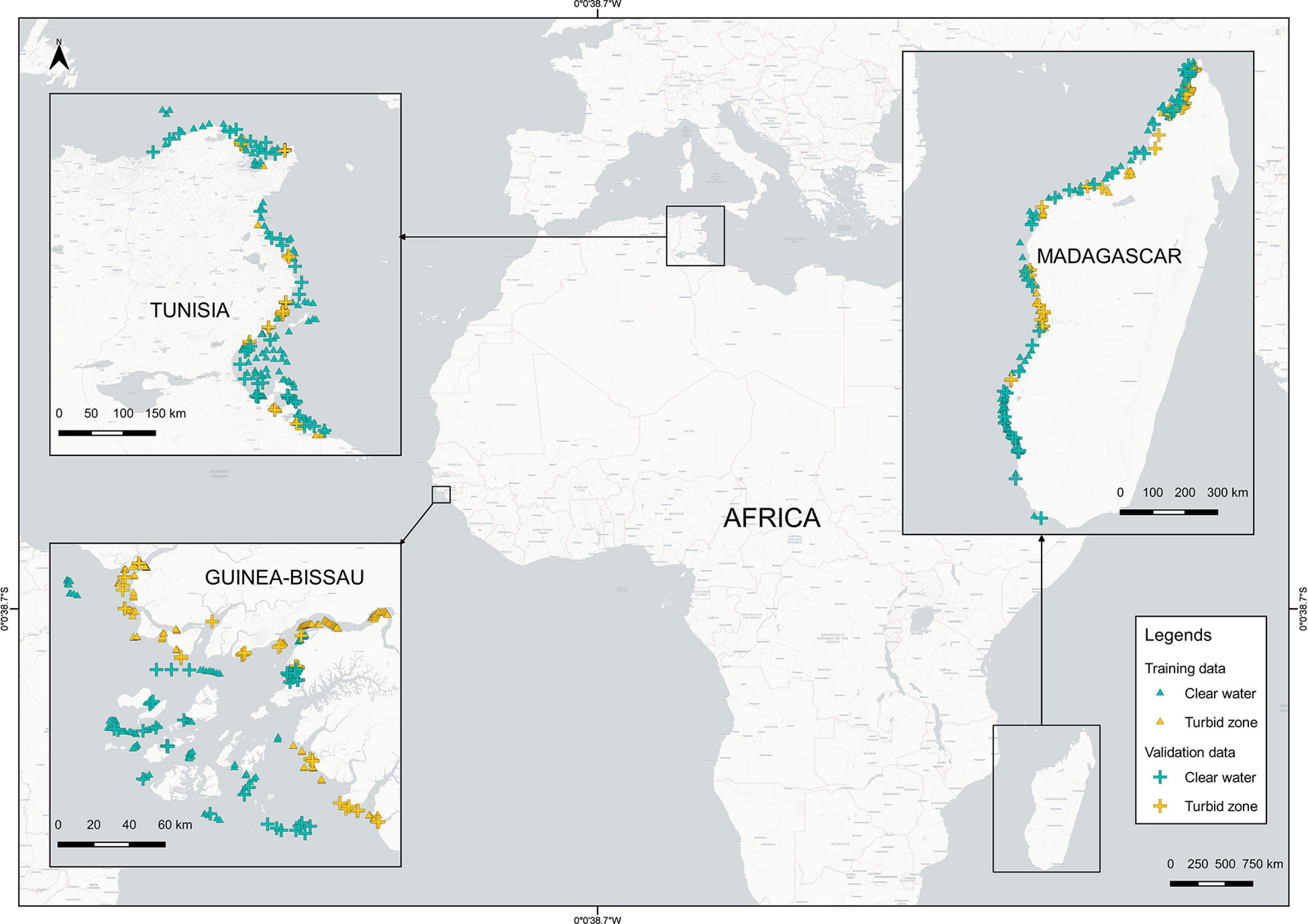
Figure 1. Map of the study regions; Guinea-Bissau, Tunisia, and the west coastline of Madagascar with annotated training and validation data points for CW and TZ (basemap by CartoDB).

Data

Sentinel-2 Level-2A Surface Reflectance Archive

This study utilized the image collection of Sentinel-2 L2A (S2 L2A) surface reflectance data available on GEE. S2 L2A images acquired between March 28, 2017 and December 3, 2020 were retrieved and synthesized. Heavily turbid water is visually distinctive through the synthesized S2 L2A RGB composite as it tends to look murky and muddy in red to brown hues as opposed to the turquoise-blue CW (subsets of the synthesized RGB composites presented in Figures 4A–C).

FIGURE 2

Figure 2. Sentinel-2 L2A water-leaving reflectance (R_hown) spectral profile of the TZ and CW training data in the three study regions: (A) Guinea-Bissau, (B) Tunisia, and (C) Madagascar.

FIGURE 3

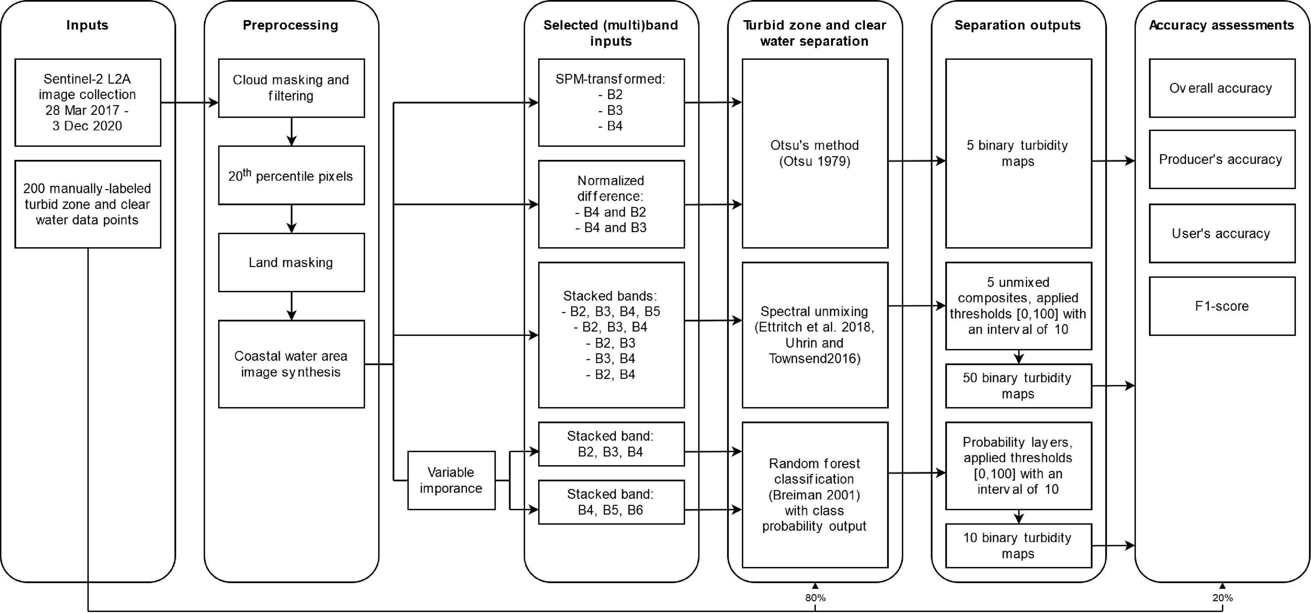
Figure 3. The flowchart of the applied methodology.

FIGURE 4

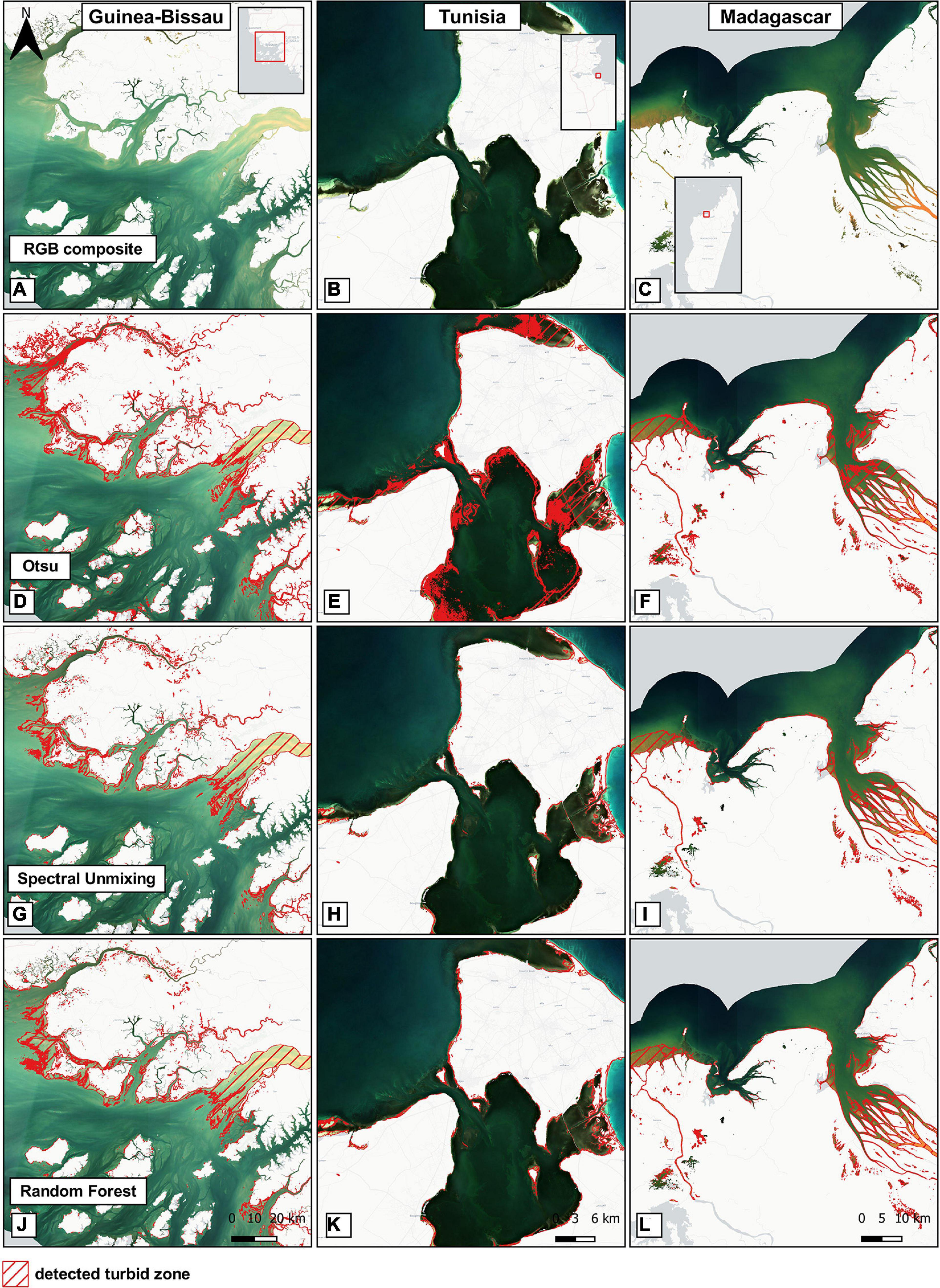
Figure 4. Subsets of the synthesized S2 L2A RGB composite of (A) Guinea-Bissau; (B) Tunisia; and (C) Madagascar study regions; (D–F) RGB composites with turbid zone detected by Otsu’s separation method on ND(B4/B2) raster; (G–I) RGB composites with turbid zone detected by spectral unmixing on B2–B5 composite; (J–L) RGB composites with turbid zone detected by Random Forest classification (base map by CartoDB).

Training and Validation Data

The training and validation datasets for the TZ and CW classes were manually digitized by observing both the synthesized S2 L2A composites and the high-resolution satellite base map on the GEE cloud platform. The datasets consist of 160 training data points and 40 validation data points in each study region—to satisfy the split proportion of 80:20, labeled to TZ and CW classes (Figure 1).

Figure 2 shows the spectral profiles of R_hown values sampled to the labeled training data points in the three study regions. CW class is represented by lower spectral values—representing the dark blue water, whereas TZ class is represented by higher spectral values—representing the lighter colors of the suspended sediments.

Methods

With the capabilities of the cloud platform GEE, it is possible to process country-scale raster images in a timely manner by offloading the heavy computational tasks to the server. We employed GEE for our end-to-end workflow which includes: image pre-processing, TZ and CW separation [using OM (Otsu, 1979), SU (Uhrin and Townsend, 2016; Ettritch et al., 2018), and RF (Breiman, 2001)], and accuracy assessments. Figure 3 shows a flowchart that systematically illustrate these methodological steps.

Image Pre-processing

The cloud-native S2 L2A image pre-processing workflow (Traganos et al., 2018) was adapted with slight modifications. GEE S2 L2A image collections retrieved and filtered by date and area were masked from cloud cover with a cloud pixel percentage filter of less than 25% as well as using the S2 L2A cloud mask (QA60) band and Scene Classification (SCL) map. Furthermore, multi-temporal data synthesis to reduce the image collections to their 20th percentile pixels was applied to reduce interferences with higher reflectance values in coastal waters such as sun glint, turbidity, waves, haze, and clouds. The land pixels were omitted using OM (Otsu, 1979) based on the modified normalized difference water index (MNDWI) (Xu, 2006), resulting in synthesized R_hown composites. Table 1 shows the specifications of S2 L2A scenes used to build the syntheses and the corresponding investigated areas.

TABLE 1

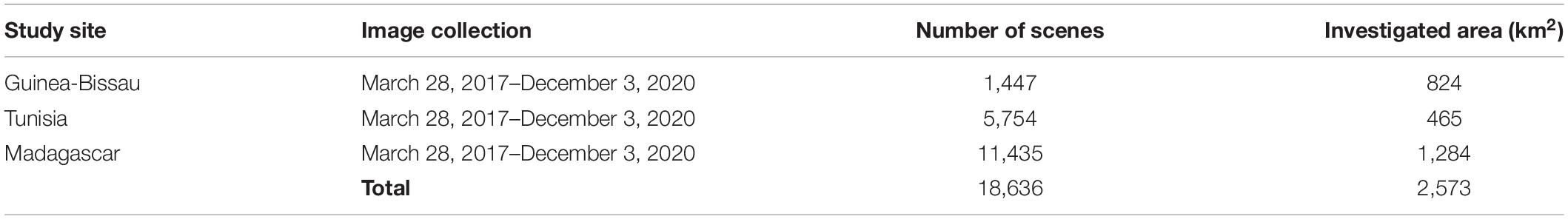
Table 1. The specifications of image collection scenes used to build the image syntheses and the investigated areas in km².

Otsu’s Method for Bimodal Thresholding

Otsu’s method (Otsu, 1979) was applied on SPM-transformed S2 L2A blue (SPM B2), green (SPM B3), red (SPM B4), red edge bands (SPM B5) (Nechad et al., 2010), normalized red-blue band difference [ND(B4/B2)] (Li et al., 2020), and normalized red-green band difference [ND(B4/B3)]. This method works for single-band images with bimodal pixel distribution by defining a minimum threshold value that separates two classes. These minimum threshold values were then readjusted in order to fit the intended borders between the TZ and CW classes, resulting in a binary turbidity map.

Linear Spectral Unmixing

Google Earth Engine’s ee.Image.unmix is a linear SU function which assumes that each class is represented by unique spectral profiles which can be summed up in a linear model to obtain the final spectral values of the raster image. The presence of each class was assumed based on their required composition in the model. The labeled training data points were used to train the model together with the sampled reflectance values. Using this method, we experimented with five combinations of S2 L2A visible band composites: (1) blue, green, red, and red edge (B2-B3-B4-B5); (2) blue, green, and red (B2-B3-B4); (3) blue and green (B2-B3); (4) green and red (B3-B4); and (5) blue and red (B2-B4). We applied the sum-to-one and non-negative constraints to the output in order to normalize the output range between 0 and 1, multiplied the resulting unmixed layers with 100 to get the value range of 0–100, and applied thresholds with the interval of 10 to produce multiple binary turbidity maps.

Random Forest Supervised Classification

The GEE smileRandomForest function with class probability layer output was selected to separate the TZ and CW classes. RF differentiates the class of the pixel using multiple decision trees (we selected 50 trees) with a voting system trained with the labeled training data and sampled reflectance values. Prior to the classification, the variable importance—which returns the sum of Gini impurity index decrease over the trees—was assessed in order to select the most relevant bands for the classification. The classification output is a raster image of class probability ranging between 0 and 100, to which we applied thresholds with the interval of 10, resulting in multiple binary turbidity maps.

Accuracy Assessments

The labeled validation datasets were used to sample all resulting binary turbidity maps and then validated. For each validation, we quantified the accuracies with error matrices and reported the results in overall accuracies (OA), producer’s accuracies (PA), user’s accuracies (UA), and F1-scores. The OA, PA, UA, and F1-scores were used as a base to determine the selected maps for further visual inspections. Visual inspections were conducted in order to check the map accuracies quantitatively as compared to the TZ seen on the synthesized S2 L2A RGB composites and the GEE high-resolution satellite base map.

Results

Table 2 shows the accuracy scores of all the attempts with the three methods and varying thresholds and band input combination. Methods and the inputs that yield the best results are highlighted in green. Based on the iterative experiments with OM and visual interpretation, ND(B4/B2) shows the best sensitivity to the intensity of turbidity, with the acquired minimum threshold value of 0.01. The OA of Guinea-Bissau and Madagascar turbidity maps are satisfactory at 85 and 95%, respectively, and the F1-scores, 0.85 and 0.95, are showing a relatively good balance between the UA and PA. However, the OA and F1-score of Tunisia turbidity map—70% and 0.69—are relatively lower because the acquired threshold value was too low for this region specifically. The threshold values were adjusted by visually observing ND(B4/B2) gradient and the synthesized S2 L2A RGB composites, resulting in the final separating thresholds of 0.02, 0.05, and 0.01 for the Guinea-Bissau, Tunisia, and Madagascar study regions, respectively. Figures 4D–F show the TZ (in red hashed red polygons) detected by OM with ND(B4/B2) input from the three study regions. As seen in Figure 4E, the TZ in Tunisia was overpredicted on the darker pixels which might represent vegetated substrates such as seagrass meadows or algae, which was not an isolated case with this band input, as it occurred with separation using other band inputs [TSM B2, TSM B3, TSM B4, TSM B5, and ND(B4/B3)]. Nevertheless, this method shows good results in the Guinea-Bissau and Madagascar study regions.

TABLE 2

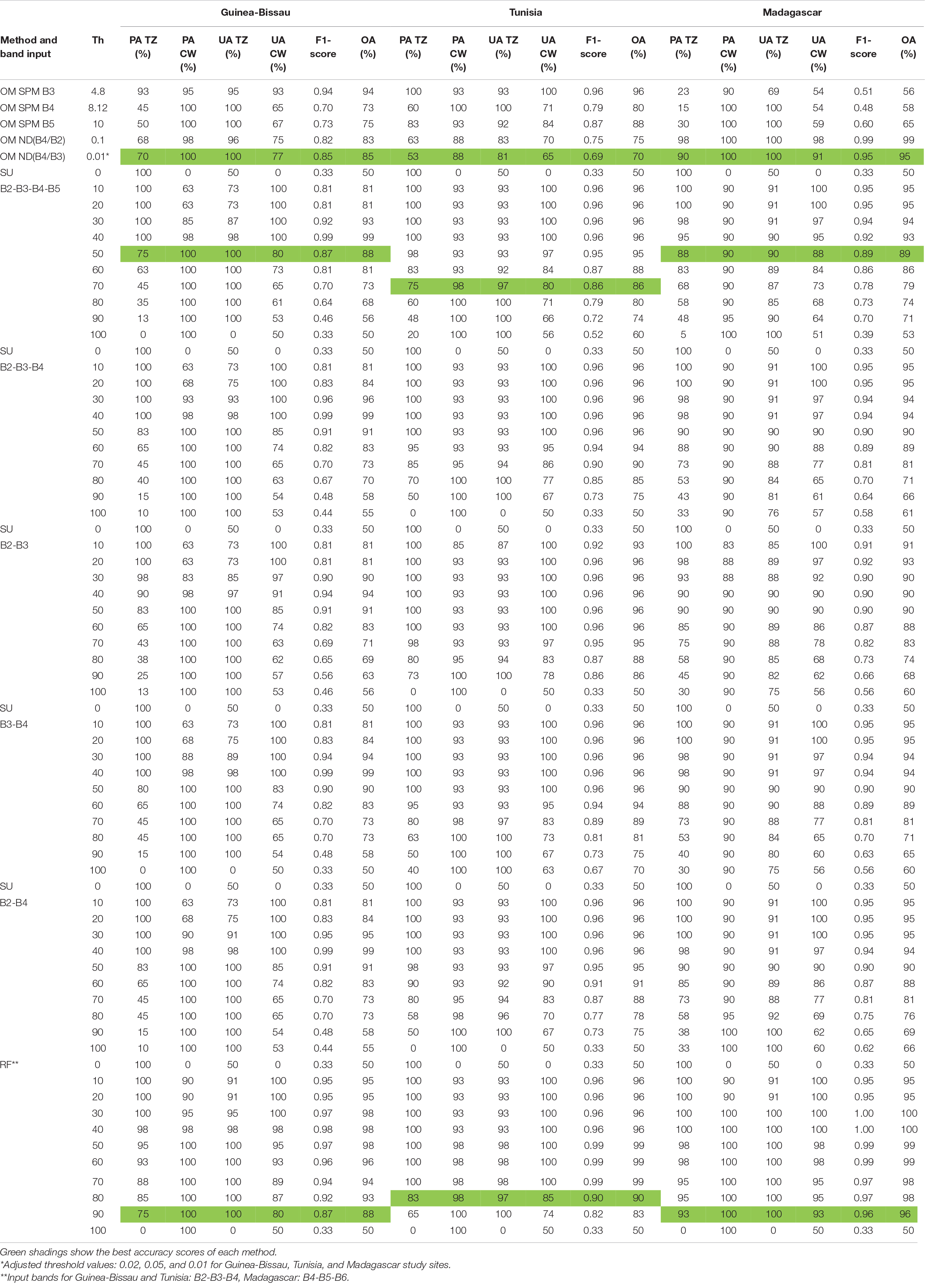
Table 2. Accuracy scores of the best turbid zone (TZ) and clear water (CW) class separation using Otsu’s method (OM), spectral unmixing (SU), and Random Forest (RF), reported in producer’s accuracies (PA), user’s accuracies (UA), F1-scores, overall accuracies (OA) in Guinea-Bissau, Tunisia, and west coastline of Madagascar study regions.

By using the SU method, the highest OA and F1-scores were achieved by applying the threshold value of 40 to the unmixed layers with the input of B2-B3-B4-B5 composite. However, further visual inspection of the resulting binary map reveals that this threshold value leads to overprediction of TZ. The unmixed layer threshold values of 50, 70, and 50 were then selected for the Guinea-Bissau, Tunisia, and Madagascar study regions, respectively, as they separated the two classes more precisely. OA and F1-scores of these three sites were close, ranging between 86 and 89% and 0.86 and 0.89 (Table 2), respectively. Figures 4G–I show the TZ detected by SU method. Unlike the results of OM, the dark pixels in Tunisia are not misclassified (Figure 4H). However, TZ in Guinea-Bissau is slightly underpredicted: shallow waters with moderate intensities of turbidity on the northwest were classified as such (Figure 4G)—which is apparent in the accuracy scores, where TZ features a PA lower than the UA, and also lower than both the PA and UA of CW.

Figure 5 presents the RF band variable importance scores of each study region. In the Guinea-Bissau study region, the red band holds the highest score in variable importance, 11.93, followed by the blue, 9.44, and the green band, 7.54. In Tunisia, the best variable importance score falls to green band, 14.31, followed by red, 12.14, and blue band, 10.61. As opposed to those regions, the importance scores of the red and the first two red edge bands in Madagascar are much higher compared to the others, 9.19, 9.67, and 11.16, whereas the scores of the blue and green bands are relatively low, 2.86 and 2.13, respectively. Therefore, we narrowed the RF band input to blue, green, and red band (B2-B3-B4) in the Guinea-Bissau and Tunisia study regions, and we narrowed down the RF band input to the red band and the first two red edge bands (B4-B5-B6) in the Madagascar study region. Figures 4J–L show the TZ detected by RF classification. RF results in more balanced prediction accuracies compared to the previous two methods: moderately turbid regions in Guinea-Bissau are masked out (Figure 4J), dark pixels in Tunisia are intact (Figure 4K), and TZ in the estuary is not overly predicted (Figure 4L). This is also reflected in the F1-scores: 0.87, 0.90, and 0.96 for Guinea-Bissau, Tunisia, and Madagascar study regions. The OA of the RF turbidity map are also relatively high: 88, 90, and 96% for the three sites (Table 2).

FIGURE 5

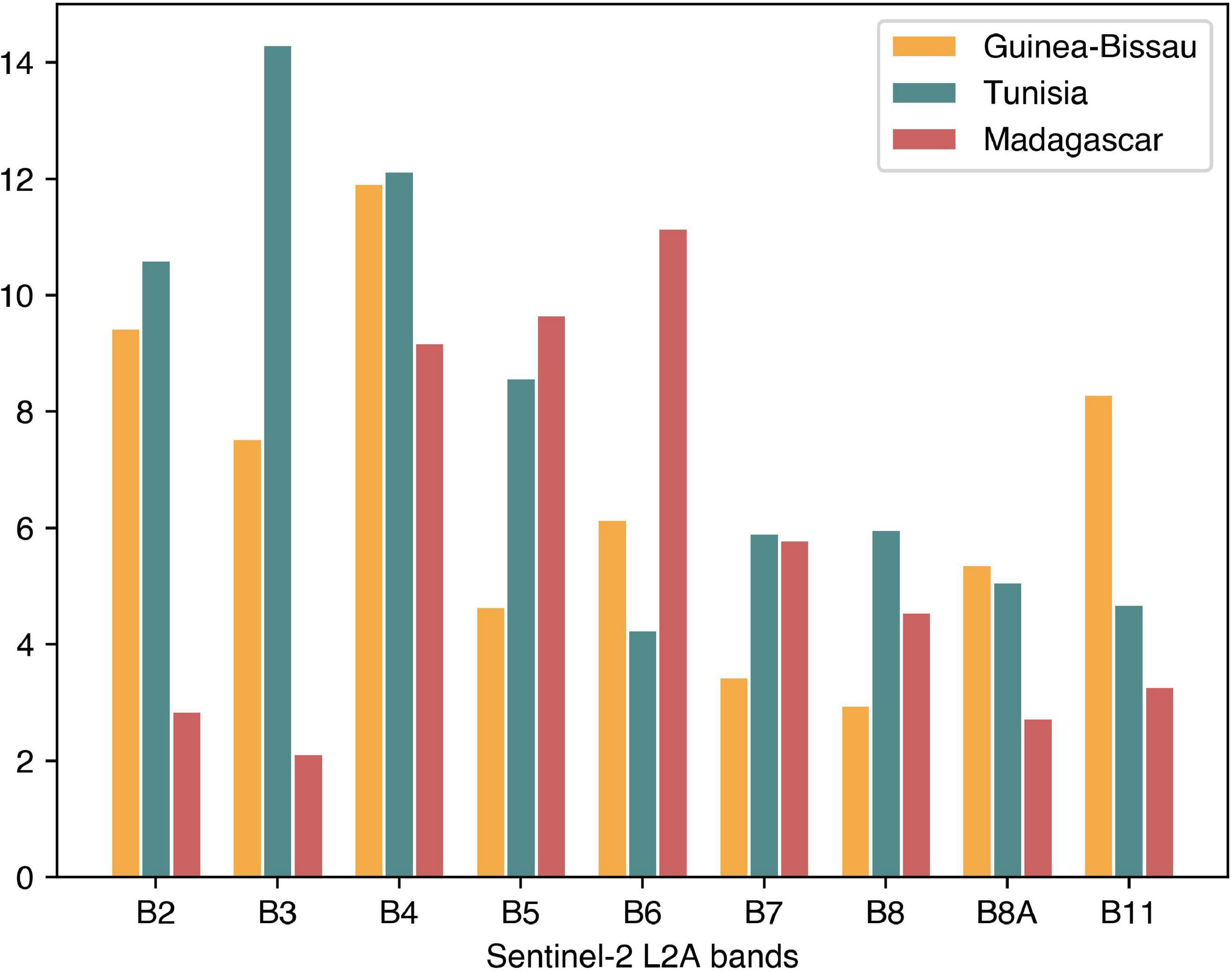
Figure 5. Random Forest Sentinel-2 L2A band variable importance for TZ and CW classification.

Discussion

In this study, we experimented on TZ detection leveraging OM (Otsu, 1979), SU (Uhrin and Townsend, 2016; Ettritch et al., 2018), and RF machine learning method (Breiman, 2001) with multi-temporal satellite data synthesis (Traganos et al., 2018) two-class separation—TZ and CW—across tropical, Mediterranean, and subtropical coastline-to-national scales in Africa. TZ detected with these three methods coincide with the highly turbid regions pointed out by previous studies along the Guinea-Bissau coastline (Vanhellemont et al., 2013), Gulf of Gabes in Tunisia (Katlane et al., 2010), and Bombetoka Bay in Madagascar (Raharimahefa and Kusky, 2010). Based on our experiments, no one method is fit-for-all due to the inter-class variability that is caused mainly by the suspended sediment compositions and the benthic substrate variability which determine the dominant colors. Additionally, the multi-temporal data synthesis method, the degree of salinity, the seabed geomorphology, the climatic conditions of the study regions, and human activities all affect the spectral histograms of these two classes as well.

RF supervised classification method works relatively well for all study regions with varying scores of spectral band importance and class probability threshold values. The variable importance graph (Figure 5) shows that red and red edge bands are more relevant to distinguish these two classes across the west Madagascar coastline as opposed to the Guinea-Bissau and Tunisia study regions where the blue, green, and red bands score higher. This might be linked to the main composition of the suspended sediments along the west coastline of Madagascar which originate from laterites—iron and aluminum-rich rocks severely transformed by tropical weathering—on the Madagascar highlands, leaving the color of the sediment dominantly in red hues (Raharimahefa and Kusky, 2010). On the other hand, the suspended sediments along the Guinea-Bissau coastline mostly consist of marine mud and fluvial sediments (Anthony, 2006), while the suspended sediments in Tunisian lagoons and gulfs are mainly accumulated from nutrients and byproducts of human activities (Ærtebjerg et al., 2001; Katlane et al., 2010; Abidi et al., 2018). The dominant color of the suspended sediments varies from light brown to brown along the Guinea-Bissau coastline and spanning from yellow to green and brown hues along the Tunisian coastline. This shows that the spectral band sensitivity to turbidity depends on the source of the suspended materials which does not only affect their colors but also their sub-pixel compositions.

In order to better understand the spectral profiles of the TZ and CW classes in these three regions, we analyzed the distributions of the pixel values representing each class. Figure 2 illustrates the distribution of the synthesized S2 L2A R_hown spectral profiles spanning from the visual bands—blue, green, red, red edge—to the NIR band based on the labeled training data. These spectral profiles show that although the TZ and CW classes have distinctive pixel values on most of the plotted bands, they share overlapping pixel values. However, these spectral profiles should be interpreted with care as they are only the statistical representatives and not the actual spectral profile of a pixel in either class. Through these spectral profiles, we also observe that in the Madagascar study region, the spectral variation between TZ and CW classes on the red and the red edge bands is much higher than their spectral variation in the other two regions. As the TZ class is represented by higher reflectance values, CW regions with shallow sandy seabed—commonly represented by higher reflectance values as well—were often misclassified as TZs. Additionally, turbidity acts as a secondary property in the form of sediments that are suspended throughout the water column. Therefore, turbid water may exist over various benthic substrates and depths. As such, improving the TZ extraction requires disentanglement of the confounding values from the primary properties (e.g., benthic substrates) as well as calibration of turbidity in order to better identify the turbid areas.

Turbid zone acquired through the OM with ND(B4/B2) and ND(B4/B3) were overpredicted because the normalized difference images fail to indicate other possible classes such as vegetated substrate which might be represented by similar spectral values. This is especially apparent in Tunisia where the dark vegetated benthic pixels are classified as TZ, which can be attributed to a source of the therein turbidity: nutrients. On the other hand, although the accuracy scores with the TSM B3, B4, and B5 were seemingly sufficient, we observed pixel misclassification in many regions as well. Although red and red edge bands by themselves are sensitive to turbidity, the information from a single band is apparently not enough to detect TZ composed by varying spectral profiles in one image. Compared to the results using OM which is reliant on a single band or a single normalized band difference input, SU and RF are more accurate—both quantitatively and qualitatively—as multiple spectral band inputs are supported, with an additional cost-benefit of requiring less manual tuning on the threshold values. With these two methods, dark pixels that might represent vegetated substrates were not falsely detected as TZ. However, these two methods were unable to resolve the overprediction of shallow sandy seabed. Furthermore, by using SU, we observe overprediction of TZ over water with low intensity of turbidity and underprediction over light-colored water with moderate intensity of turbidity in Guinea-Bissau and Madagascar study regions. By using RF, the feature—in this case, the spectral band—importance can be easily assessed, making it easier to narrow down the most relevant bands to distinguish the classes. With RF, overprediction occurred mostly in slightly turbid water regions.

Other factors that might affect the accuracy are the multi-temporal synthesis, salinity, seabed geomorphology, climatic conditions of the study regions, and human activities. Here, we performed multi-temporal synthesis using the 20th percentile of over 25 billion pixels of more than 18,600 cloud-filtered S2 L2A scenes which results in synthetic images with of darkest pixels across the selected satellite time series. As a result, seasonal turbid regions might have been omitted from the final syntheses. With this synthesis method, we did not acquire the ephemeral TZ, but detected only TZ which are consistent throughout the time period of the satellite syntheses (Table 1). Seasonal TZ detection can be performed by selecting monthly to seasonal time windows to conduct the in contrast to the 3-year time windows here. However, as a tradeoff, other optical interferences like clouds, especially in tropical and subtropical regions, might impede the smaller time windows and syntheses. Seawater salinity also affects the light attenuation in these three regions. Mediterranean seas are relatively of higher salinity than those of the Guinea-Bissau and Madagascar coastlines, affecting the spectral profiles and the color variations. Moreover, the seabed geomorphology and climatic conditions such as the sun zenith angles, the intensity of the sunlight, the temperature, persistent cloud covers, and the rainfall intensity also affect the spectral profiles of the final syntheses. Human activities in the proximity of the study regions contribute to the main constituents of the suspended sediments in the rivers, river estuaries, and coastlines. An improved tuning of these factors can be performed by using ground-truth data, through which the training and validation data can be further calibrated.

Conclusion

The aim of this study is to evaluate the accuracy and the scalability of three different methods to detect non-seasonal TZs of wide-ranging magnitude and composition. We experimented with OM, linear SU, and RF to detect the TZ in three study sites in tropical (Guinea-Bissau), Mediterranean (Tunisia), and subtropical (Madagascar) climate regions. TZs detected by these three methods coincide with the primarily turbid regions pointed out by previous studies. TZ detection is highly site-specific, depending highly on the compositions of the suspended materials and the variability of the benthic substrate. The compositions of the suspended materials depend heavily on the land surface geomorphology, human activities, and the soil nutrients. Additionally, at a lesser extent, the multi-temporal synthesis, seawater salinity, seabed geomorphology, the climatic conditions, and human activities are also affecting the dominant colors of the sediments and the whole aquatic ecosystem. Based on our experiments with these three methods, adjustments in input and threshold values were still needed prior to and after the classification. RF produced the best result both quantitatively and qualitatively, with automated assessments of the spectral band importance, with the F1-scores of 0.87, 0.90, and 0.96 and the OA of 88, 90, and 96% for Guinea-Bissau, Tunisia, and Madagascar study regions, respectively. The result of this study can support relevant coastal aquatic remote sensing studies, such as benthic habitat and SDB mapping, where one can mask out the TZ and focus the mapping on the CW regions where the light attenuation is not disturbed. Accurate TZ detection can better inform coastal aquatic ecology and decision making on suitable areas to rehabilitate the water quality.

Data Availability Statement

Publicly available datasets were analyzed in this study. This data can be found here: https://scihub.copernicus.eu/.

Author Contributions

AP and DT contributed to conception and design of the study. AP and CL developed the methodology algorithms. All authors contributed to manuscript revision, read, and approved the submitted version.

Funding

AP and DT acknowledge funding for their efforts from the German Aerospace Center (DLR) through the Global Seagrass Watch project. CL was supported by the DLR/DAAD Research Fellowship No. 57478193.

Conflict of Interest

The authors declare that the research was conducted in the absence of any commercial or financial relationships that could be construed as a potential conflict of interest.

Publisher’s Note

All claims expressed in this article are solely those of the authors and do not necessarily represent those of their affiliated organizations, or those of the publisher, the editors and the reviewers. Any product that may be evaluated in this article, or claim that may be made by its manufacturer, is not guaranteed or endorsed by the publisher.

References

Abidi, M., Amor, R. B., and Moncef, G. (2018). Assessment of the Trophic Status of the South Lagoon of Tunis (Tunisia, Mediterranean Sea): geochemical and Statistical Approaches. J. Chem. 2018:9859546. doi: 10.1155/2018/9859546

CrossRef Full Text | Google Scholar

Ærtebjerg, G., Carstensen, J., Dahl, K., Hansen, J., Nygaard, K., Rygg, B., et al. (2001). Eutrophication in Europe’s Coastal Waters. Copenhagen: European Environment Agency.

Google Scholar

Anthony, E. (2006). The muddy tropical coast of West Africa from Sierra Leone to Guinea-Bissau: geological heritage, geomorphology and sediment dynamics. Africa Geosci. Rev. 13, 227–237.

Google Scholar

Breiman, L. (2001). Random Forests. Machine Learn. 45, 5–32. doi: 10.1023/A:1010933404324

CrossRef Full Text | Google Scholar

Caballero, I., and Stumpf, R. P. (2020). Towards Routine Mapping of Shallow Bathymetry in Environments with Variable Turbidity: contribution of Sentinel-2A/B Satellites Mission. Remote Sens. 12:451. doi: 10.3390/rs12030451

CrossRef Full Text | Google Scholar

Caballero, I., Stumpf, R. P., and Meredith, A. (2019). Preliminary Assessment of Turbidity and Chlorophyll Impact on Bathymetry Derived from Sentinel-2A and Sentinel-3A Satellites in South Florida. Remote Sens. 11:645. doi: 10.3390/rs11060645

CrossRef Full Text | Google Scholar

Dogliotti, A. I., Ruddick, K. G., Nechad, B., Doxaran, D., and Knaeps, E. (2015). A single algorithm to retrieve turbidity from remotely-sensed data in all coastal and estuarine waters. Remote Sens. Environ. 156, 157–168. doi: 10.1016/j.rse.2014.09.020

CrossRef Full Text | Google Scholar

Ettritch, G., Bunting, P., Jones, G., and Hardy, A. (2018). Monitoring the coastal zone using earth observation: application of linear spectral unmixing to coastal dune systems in Wales. Remote Sens. Ecol. Conserv. 4, 303–319. doi: 10.1002/rse2.79

CrossRef Full Text | Google Scholar

EU (2008). Directive 2008/56/EC of the European Parliament and of the Council of 17 June 2008 establishing a framework for community action in the field of marine environmental policy (Marine Strategy Framework Directive). Official J. Eur. Union 164, 19–40.

Google Scholar

Feng, J., Chen, H., Zhang, H., Li, Z., Yu, Y., Zhang, Y., et al. (2020). Turbidity Estimation from GOCI Satellite Data in the Turbid Estuaries of China’s Coast. Remote Sens. 12:3770. doi: 10.3390/rs12223770

CrossRef Full Text | Google Scholar

Jafar-Sidik, M., Gohin, F., Bowers, D., Howarth, J., and Hull, T. (2017). The relationship between Suspended Particulate Matter and Turbidity at a mooring station in a coastal environment: consequences for satellite-derived products. Oceanologia 59, 365–378. doi: 10.1016/j.oceano.2017.04.003

CrossRef Full Text | Google Scholar

Katlane, R., Nechad, B., Ruddick, K., and Zargouni, F. (2010). Optical remote sensing of the Gulf of Gabès – relation between turbidity, Secchi depth and total suspended matter. Ocean Sci. Discuss. 7, 1767–1783. doi: 10.5194/osd-7-1767-2010

CrossRef Full Text | Google Scholar

Li, J., Knapp, D. E., Fabina, N. S., Kennedy, E. V., Larsen, K., Lyons, M. B., et al. (2020). A global coral reef probability map generated using convolutional neural networks. Coral Reefs 39, 1805–1815. doi: 10.1007/s00338-020-02005-6

CrossRef Full Text | Google Scholar

Nahirnick, N. K., Reshitnyk, L., Campbell, M., Hessing-Lewis, M., Costa, M., Yakimishyn, J., et al. (2019). Mapping with confidence; delineating seagrass habitats using Unoccupied Aerial Systems (UAS). Remote Sens. Ecol. Conserv. 5, 121–135. doi: 10.1002/rse2.98

CrossRef Full Text | Google Scholar

Nechad, B., Ruddick, K. G., and Park, Y. (2010). Calibration and validation of a generic multisensor algorithm for mapping of total suspended matter in turbid waters. Remote Sens. Environ. 114, 854–866. doi: 10.1016/j.rse.2009.11.022

CrossRef Full Text | Google Scholar

Otsu, N. (1979). A Threshold Selection Method from Gray-Level Histograms. IEEE Trans. Syst. Man Cybern. 9, 62–66. doi: 10.1109/TSMC.1979.4310076

CrossRef Full Text | Google Scholar

Raharimahefa, T., and Kusky, T. (2010). Environmental monitoring of Bombetoka Bay and the Betsiboka Estuary, Madagascar, using multi-temporal satellite data. J. Earth Sci. 21, 210–226. doi: 10.1007/s12583-010-0019-y

CrossRef Full Text | Google Scholar

Robert, E., Kergoat, L., Soumaguel, N., Merlet, S., Martinez, J. M., Diawara, M., et al. (2017). Analysis of Suspended Particulate Matter and Its Drivers in Sahelian Ponds and Lakes by Remote Sensing (Landsat and MODIS): Gourma Region, Mali. Remote Sens. 9:1272. doi: 10.3390/rs9121272

CrossRef Full Text | Google Scholar

Ruescas, A. B., Hieronymi, M., Koponen, S., Kallio, K., and Camps-Valls, G. (2017). “Retrieval of coloured dissolved organic matter with machine learning methods,” in 2017 IEEE International Geoscience and Remote Sensing Symposium (IGARSS), (New York: IEEE), 2187–2190.

Google Scholar

Sebastiá-Frasquet, M. T., Aguilar-Maldonado, J. A., Santamaría-Del-Ángel, E., and Estornell, J. (2019). Sentinel 2 Analysis of Turbidity Patterns in a Coastal Lagoon. Remote Sens. 11:2926. doi: 10.3390/rs11242926

CrossRef Full Text | Google Scholar

Stramski, D., Boss, E., Bogucki, D., and Voss, K. J. (2004). The role of seawater constituents in light backscattering in the ocean. Prog. Oceanogr. 61, 27–56. doi: 10.1016/j.pocean.2004.07.001

CrossRef Full Text | Google Scholar

Traganos, D., Aggarwal, B., Poursanidis, D., Topouzelis, K., Chrysoulakis, N., and Reinartz, P. (2018). Towards Global-Scale Seagrass Mapping and Monitoring Using Sentinel-2 on Google Earth Engine: the Case Study of the Aegean and Ionian Seas. Remote Sens. 10:1227. doi: 10.3390/rs10081227

CrossRef Full Text | Google Scholar

Uhrin, A., and Townsend, P. (2016). Improved Seagrass Mapping Using Linear Spectral Unmixing of Aerial Photographs. Estuar. Coast. Shelf Sci. 171, 11–22. doi: 10.1016/j.ecss.2016.01.021

CrossRef Full Text | Google Scholar

Vanhellemont, Q. (2019). Daily metre-scale mapping of water turbidity using CubeSat imagery. Opt. Express 27, A1372–A1399. doi: 10.1364/OE.27.0A1372

PubMed Abstract | CrossRef Full Text | Google Scholar

Vanhellemont, Q., Neukermans, G., and Ruddick, K. (2013). “High frequency measurement of suspended sediments and coccolithophores in European and African coastal waters from the geostationary SEVIRI sensor,” in Proceedings of the EUMETSAT Meteorological Satellite Conference 19th American Meteorological Society (AMS) Satellite Meteorology, Oceanography, and Climatology Conference, Vienna, Austria, (Massachusetts: American Meteorological Society (AMS)).

Google Scholar

Vela, A., Pasqualini, V., Leoni, V., Djelouli, A., Langar, H., Pergent, G., et al. (2008). Use of SPOT 5 and IKONOS imagery for mapping biocenoses in a Tunisian Coastal Lagoon (Mediterranean Sea). Estuar. Coast. Shelf Sci. 79, 591–598. doi: 10.1016/j.ecss.2008.05.014

CrossRef Full Text | Google Scholar

Xu, H. (2006). Modification of normalised difference water index (NDWI) to enhance open water features in remotely sensed imagery. Int. J. Remote Sens. 27, 3025–3033. doi: 10.1080/01431160600589179

CrossRef Full Text | Google Scholar