 Jonathan Tinker
 Leon Hermanson
- Met Office Hadley Centre, Exeter, United Kingdom
We investigate the winter predictability of the North West European shelf seas (NWS), using the Met Office seasonal forecasting system GloSea5 and the Copernicus NWS reanalysis. We assess GloSea5’s representation of NWS climatological winter and its skill at forecasting winter conditions on the NWS. We quantify NWS winter persistence and compare this to the forecast skill. GloSea5 simulates the winter climatology adequately. We find important errors in the residual circulation (particularly in the Irish Sea) that introduce temperature and salinity biases in the Irish Sea, English Channel, and southern North Sea. The GloSea5 winter skill is significant for SST across most of the NWS but is lower in the southern North Sea. Salinity skill is not significant in the regions affected by the circulation errors. There is considerable NWS winter temperature and salinity persistence. GloSea5 exhibits significant predictive skill above this over ∼20% of the NWS, but for most of the NWS this is not the case. Dynamical downscaling is one method to improve the GloSea5 simulation of the NWS and its circulation, which may reduce biases and increase predictive skill. We investigate this approach with a pair of case studies, comparing the winters of 2010/2011 and 2011/2012 (with contrasting temperature and salinity anomalies, and NAO state). While 2 years are insufficient to assess skill, the differences in the simulations are evaluated, and their implications for the NWS winter predictability are considered. The NWS circulation is improved (where it was poor in the GloSea5), allowing more realistic advective pathways for salinity (and temperature) and enhancing their climatological spatial distributions. However, as the GloSea5 SST anomaly is already well simulated, downscaling does not substantially improve this – in other seasons or for other variables, downscaling may add more value. We show that persistence of early winter values provides some predictive skill for the NWS winter SST, and that the GloSea5 system adds modestly to this skill in certain regions. Such information will allow prospective end-users to consider how seasonal forecasts might be useful for their sector, providing the foundation on which marine environmental seasonal forecasts service and community may be developed for the NWS.
Introduction
The North West European Shelf Seas (NWS) are a broad set of shallow seas to the northwest of Europe and surrounding the British Isles. Their large area and shallow depth lead to large tides which dominate the local oceanography. They border several populous countries and support a wide range of economic interests, including fisheries, the oil and gas industry, shipping and transport, renewable energies, and leisure, and are environmentally important. They are managed and protected with a wide range of legislation at the international, European, national, and local levels.
In order to best protect, manage and utilise the NWS, predictions and projections of their future state are important. Currently there is a suite of predictions for the synoptic scale and projections for the end of century, but there are no predictions for the intermediate timescales. Reanalyses are now available for the NWS, which assimilate observations to enhance the simulation of the recent past – these give the best estimate of the state of the NWS. For example, the Met Office reanalysis (1993-2018) is freely distributed by the Copernicus Marine Environmental Monitoring Service (CMEMS) – this includes temperature, salinity, currents, water column structure (Renshaw et al., 2019). Such reanalyses are ideal for assessing the local climatology, interannual variability, and to act as pseudo-observations in observation poor environments. Operational oceanographic forecasts are closely related to reanalyses and are also available. CMEMS disseminates the Met Office 6-day operational forecast (Tonani et al., 2019) for the NWS, which includes similar parameters. Uninitialised climate projection are available for the NWS, which focus on the end of the 21st century (e.g., Tinker et al., 2016). With care, these can be used earlier in the 21st century if the climate signal has emerged from the climate variability, however the near-term period months or years ahead will be dominated by internal variability, leading to a requirement for initialised predictions.
The monthly-to-decadal (m2d) time scale is of particular interest to end users, as it is the time scale on which fishers might decide to buy a new boat, managers decide to close a fishing ground, etc. Short-term forecasts for the next week rely heavily on the initial conditions at the beginning of the forecast, but become increasingly decorrelated from the initial conditions with lead time due to their chaotic nature. The uninitialised climate projections rely on the climate change signal being greater than the climate variability, and so are not designed for predicting the immediate future. Between these time scales, m2d predictions can derive skill from both initial conditions and external forcings and although they cannot be used to predict the weather of a particular day, they can indicate the general characteristics of a season. Here we focus on the seasonal time scale.
Operational global seasonal forecasting systems (such as the Met Office’s GloSea5 system, MacLachlan et al., 2014) and multi-model ensemble systems operate on seasonal timescales. They combine coupled global climate models with data assimilation and observationally constrained initial conditions. GloSea5 has demonstrated significant skill at predicting the European winter conditions, through skilful prediction of the North Atlantic Oscillation (NAO) from the previous November (Scaife et al., 2014). The NAO is a key determinant of the nature of the European winter (e.g., Hurrell, 1995) with a positive NAO index indicating mild, wet conditions and a negative NAO index indicating cold, dry conditions. This predictive skill has been exploited to demonstrate predictability in a number of user-relevant variables, e.g., relating the phase of the NAO index to the likely number of transport disruption (road, rail, and air) impacts (Palin et al., 2016) or to hydrological or energy impacts (Svensson et al., 2015; Clark et al., 2017), but so far there has been less attention to seasonal predictability of NWS marine variables (e.g., Hobday et al., 2016).
While global seasonal forecasting systems can simulate important aspects of the weather, climatic and even open ocean conditions, there are complications with their representation of shelf seas conditions. The ocean component of these global seasonal forecasting systems is not optimised for the NWS, having insufficient resolution (0.25 degrees here), and missing important processes (such as dynamic tides). Therefore, they do not simulate important aspects of the NWS well. For example, in reality tidal mixing does not allow complete summer stratification on the NWS, as large parts of the southern North Sea, the English Channel and Irish Sea remain fully mixed though the year. In GloSea5, these regions are predominantly stratified in summer (Tinker et al., 2018) – as the pattern of seasonally stratified and fully mixed regions, and the fronts between them, are so important for the dynamics of the NWS this is a major limitation. Tides also modify the mean residual circulation (e.g., Robinson, 1983), which has important implications for the distribution of tracers.
In recent years the number of marine seasonal forecasting products (often with an ecological application) has rapidly increased, although there have been few for European waters (Payne et al., 2017). Australia (Hobday et al., 2011; Eveson et al., 2015; Brodie et al., 2017) and the United States (Anderson and Beer, 2009; Burke et al., 2013; Kaplan et al., 2016; Mills et al., 2017; Liu et al., 2018) have been at the forefront of such development. At present there have been no such products for the NWS. The seas around Australia and the United States tend to be better resolved (in global models) than the NWS, and both have Pacific coastlines, where the ENSO lends additional predictability. Furthermore, both the Australian and American fisheries are managed by a single national agency, which may allow a more flexible and rapid response to new opportunities than is possible in Europe, where fisheries management needs to balance the interests of many different nations (Payne et al., 2017). However, Europe is adjacent to the North Atlantic subpolar gyre (which is predictable on decadal timescales) and is controlled by the NAO, which is predictable on the seasonal time-scale. These, along with a long history of scientific investigation of fish stock productivity (e.g., Hjort, 1914), make the NWS a fertile ground for the development of such products (Payne et al., 2017).
Although there are aspects of the NWS that are not simulated well by global seasonal forecast systems, Tinker et al. (2018) explored how to use such systems as the basis of NWS seasonal forecasts. They outlined three approaches: (1) direct use of model output from a seasonal forecast system; (2) statistical downscaling of a seasonal forecast system; and (3) dynamical downscaling a seasonal forecasting system. They showed that (1), the direct use of GloSea5 would not be advisable for all locations and times, particularly in the summer (due to poorly resolved stratification, see above), and for salinity (due to river outflow). Tinker et al. (2018) explored (2), and showed that for some parameters and places, statistical downscaling can provide significant skill at lead time of a few months, based on GloSea5 predictability and persistence within the system. They did not assess the skill associated with dynamical downscaling, but highlight the boundary-constrained nature of the NWS which supports the possibility of dynamically downscaled seasonal forecasts.
In this study we further assess the skill of GloSea5 at representing and predicting winter conditions on the NWS. During winter the NAO is predictable and has the greatest impact on European climate. Furthermore, atmospheric conditions fully mix the winter NWS (apart from the adjacent salinity stratified Norwegian Trench, and small coastal regions), and so winter tidal mixing is less important – the NWS can be considered in its simplest state. We show where and what GloSea5 can represent and predict, and why it is less successful with some aspects of the NWS winter. We quantify the inherent persistence of the NWS winter, and compare the GloSea5 skill to this persistence. We then use a pair of case studies to begin to assess how dynamical downscaling alters predictions of the NWS. In this study, we focus on temperature and salinity. The scientific questions we aim to address are:
• How well does GloSea5 simulate the climate of the NWS winter?
• How well does GloSea5 predict winter variations on the NWS?
◦ Which NWS variables are predictable by GloSea5 and where?
• How persistent are NWS winter conditions?
◦ Does GloSea5 skill beat this persistence?
• How does dynamical downscaling affect prediction?
◦ How does it affect the spatial pattern and temporal evolution?
In the following Methods section we describe the models, experimental design and some of the techniques used in this study. In the Results sections we address the questions above, before discussing the results, and their underlying drivers in the Discussion section.
Models and Methods
GloSea5
GloSea5 (MacLachlan et al., 2014) is based on the Met Office Hadley Centre climate model HadGEM3-GC2 (Williams et al., 2015). This is a coupled climate model combining the MetUM atmosphere model (N216, ∼0.7° horizontal resolution; Walters et al., 2011; Brown et al., 2012), the ocean model NEMO (Megann et al., 2014), the land surface scheme JULES (Best et al., 2011), and the sea ice model CICE (Hunke and Lipscomb, 2010). The ocean model component is run on the ORCA025 grid – a 0.25 ° tri-polar grid (∼27 km at the Equator, ∼17 km on the NWS) with 75 horizontal z-layers, of which 18 (24) are within the top 50 m (100 m). NEMO ORCA025 is run with a data analysis system (3D-Var) to assimilate a range of observations, including SST, sea surface height, sea ice concentration, and water column structure. GloSea5 use the TRIP river routing scheme (Oki and Sud, 1998; Oki et al., 1999) to return land surface water runoff back into the sea. TRIP is run on a 1 × 1° grid, with the outflow at the river mouths regridded onto the ORCA025 ocean grid (Supplementary Figure 11g). Given the coarse nature of the TRIP grid, there are no rivers that flow into the Irish Sea or English Channel, and the river mouths are located in the sea, rather than the coast.
GloSea5 seasonal forecasts are made by comparing a set of ensemble forecasts to a set of ensemble hindcasts which define the GloSea5 climatology and are used to correct model biases and drifts. The winter hindcasts are a 7-member ensemble starting on four November start dates (1st, 9th, 17th, and the 25th of the month) and each run until the 31st of May the following year. The ensemble members on each start date differ by a stochastic perturbation in the atmosphere. The hindcasts provide a consistent set of simulations over 23 years (1994-2016), and we use the set run in 2018 (the latest complete set when this study was begun) in our investigation. To produce a forecast, GloSea5 initialises two forecast ensemble members every day, which are run forward for 216 days. The previous 3 weeks are combined to make a 42-member lagged ensemble for the 6-month forecast – this is updated every week. This forecast ensemble is compared to the hindcast ensemble (which acts as a climatology), to allow anomalies to be forecast. GloSea5 is also run continuously (without an atmospheric component) from 1990 to 2016 as the GloSea5 ocean and sea ice global reanalysis – this provides initial conditions for the ocean component of the hindcast ensemble. The atmospheric initial conditions for the forecast are taken from the Met Office operational weather forecast system, and the hindcast atmosphere is initialised from ERA-Interim. See MacLachlan et al. (2014) for further details.
GloSea5 shows improved year-to-year predictions of the major modes of variability compared to the previous system (GloSea4, Arribas et al., 2011). Predictions of the El Niño–Southern Oscillation are improved with reduced errors in the western Pacific. GloSea5 shows high forecast skill and reliability for both the NAO and the Arctic Oscillation (MacLachlan et al., 2014; Scaife et al., 2014).
CMEMS v4 NWS Reanalysis (CMEMS)
The Met Office provides a NWS reanalysis to the Copernicus Marine Environment Monitoring Service1 which has been extensively described and validated (O’Dea et al., 2017; Renshaw et al., 2019). Here we use the CMEMS version 4 Reanalysis (referred to as CMEMS) - version 5 is now available.
The CMEMS v4 reanalysis is based on the NEMO coastal ocean model version 6 (CO6) implementation. This is on a regional 7 km grid extending from 40°4′N 19°W to 65°N 13°E, with 50 terrain-following levels (Siddorn and Furner, 2013). The simulations run from 1992 to 2018 (we use 1994 to 2016). The model surface forcings were calculated with the Coordinated Ocean Research Experiments (CORE) bulk formulae (Large and Yeager, 2009) using ERA-Interim data (ERAI; Dee et al., 2011). The ocean lateral boundary forcings were taken from the GloSea5 ocean reanalysis. The Baltic Sea boundary was treated as an open ocean lateral boundary, with data (temperature and salinity only) provided by another CMEMS product2 (Axell et al., 2017). Freshwater inflow into the model from rivers and other sources was prescribed from a climatology of daily discharge data for 279 rivers from the Global River Discharge Data Base (Vörösmarty et al., 2000) and from data prepared by the Centre for Ecology and Hydrology as used by Young and Holt (2007). The CO6 reanalysis assimilates sea surface temperature (SST) from satellites and in situ temperature and salinity profiles (although these are mainly in the ocean adjacent the NWS).
NEMO Coastal Ocean Version 6 (CO6)
NEMO Coastal Ocean model version 6 (CO6) implementation (O’Dea et al., 2017) is the shelf seas model used to dynamically downscale GloSea5 in our case studies. It is a primitive equation, Boussinesq, 3D baroclinic model, with a non-linear free surface. CO6 is run on a regional ∼7 km grid extending from 40°4′N 19°W to 65°N 13°E, with 50 hybrid terrain following vertical levels (Siddorn and Furner, 2013) – this is the same grid as used by the CMEMS v4 reanalysis. This resolution is insufficient to resolve the internal (baroclinic) Rossby Radius on the shelf (which is of the order 4 km) but resolves the external (barotropic) Rossby Radius (∼200 km). 15 tidal constituents are added to the ocean lateral boundary conditions, and as the model domain is relatively large, the tidal generating force is added in the model interior for the same 15 constituents. The inverse barometer effect is modelled directly and is also applied to the lateral ocean boundary conditions.
CO6 is a well-established and evaluated model, with a wide range of uses. It is used as a research model, as the basis of the Met Office operational 6-day NWS forecasts (and delivered to CMEMS3, Tonani et al., 2019), the CMEMS v4 (and v5) reanalyses (also delivered to CMEMS, Renshaw et al., 2019), and in climate research (e.g., Hermans et al., 2020; Tinker et al., 2020; King et al., 2021; Nagy et al., 2021).
We use CO6 to dynamically downscale GloSea5 – these simulations are referred to as CO6. We downscale GloSea5 opportunistically, using archived scheduled operational data, rather than customising and re-running the system with our preferred output. Therefore, we do not have our preferred temporal resolution for our boundary conditions (e.g., daily mean radiative fluxes). We use the ocean and atmosphere boundary conditions directly from GloSea5 and use climatological river forcings (the same used for the CMEMS v4 reanalysis) and Baltic exchange forcings (see Tinker et al., 2020). The atmospheric surface forcings are daily mean radiative fluxes, precipitation and evaporation, and 6 hourly wind and pressure data. Therefore, we do not simulate the diurnal cycle. We take monthly mean temperature, salinity, barotropic current and surface elevation from the GloSea5 ocean. We take our initial conditions from the CMEMS v4 reanalysis. Taking the restarts from the GloSea5 system may have been more appropriate, however the geography and dynamics are so different from CO6, that the whole 6-month run would be spinning up. As the GloSea5 reforecast is initialised from the GloSea5 ocean reanalysis, which provides the boundary conditions for the CMEMS v4 Reanalysis, it was appropriate. However, there will be an issue with persistence in the downscaled simulations, which may be of be particular importance for salinity which is slower to respond to surface forcings. Each of the 7 ensemble-members for each restart day have the same ocean initial conditions.
Persistence
For a forecast to be considered useful it is often compared to persistence, i.e., a simple prediction assuming the anomalies at the start of the forecast (relative to seasonal climatology) persisted into the future. We calculate the NWS persistence by correlating the November monthly means from CMEMS against the following winter mean values (December-February). This is compared to the deterministic skill (the correlation between the GloSea5 ensemble mean and CMEMS). This is Eulerian Persistence, where no account of advection is made. When we refer to persistence without specifying whether it is Eulerian or Lagrangian persistence, we refer to Eulerian persistence.
As the downscaled simulations take their initial conditions from CMEMS, a portion of persistence will be included in apparent model performance. This must be considered when considering the downscaled simulations, however, as we cannot assess the deterministic skill of 2 years, this point is moot.
Lagrangian Persistence
Lagrangian Persistence takes account of advection (Berndtsson et al., 1994). We use a simple method to advect the November monthly mean temperature and salinities based on a simple particle tracking algorithm (without a stochastic random walk to simulate diffusion). We use climatological depth-mean currents from CMEMS, with a seasonal cycle. We seed 400 particles in each grid box on November 15th, and advect them with the flow, updating their position every time step, using a forward difference scheme:
Where U and V are the depth mean velocities (m/s) bi-linearly interpolated to the particle location (with zero land velocities, and NaN around the domain boundary), dt is the time step (86400 seconds), and dx, dy is the change in position of the particle (m). This is converted to a change in longitude and latitude (in degrees) as:
Where R⊕ is the radius of the Earth (taken from the NEMO code as 6,371,229 m) and λ is the current latitude (in degrees).
The location of the particles is noted in the middle of December, January and February. The new particle locations for each month, with their associated November temperature and salinity data, are interpolated onto the model grid using an unstructured linear interpolation method. The new simulated December, January and February fields are averaged into a winter mean field for each year of the CMEMS reanalysis and are correlated against the November fields.
The results are relatively insensitive of time step (we use dt = 86400 s (1 day), but had similar results from 1, 2, 4, 6, 8, and 12 h time steps) and number of particles seeded per grid box (we tested with 1, 2, 4, 100, and 400, but use 400). We also had similar results from using a NWS current climatology from a present day control simulation (Tinker et al., 2020), and from using the particle tracking package OpenDrift (Dagestad et al., 2018), with hourly tidal data from Tinker et al. (2020).
Data Description and Significance Testing
When comparing spatial patterns (Figures 1, 9) we use the bias, the correlation (r) and relative standard deviation (rsd, the standard deviation of GloSea5/CO6 divided by that of CMEMS) (following Taylor, 2001). We also use r and rsd to compare time-series (Figures 4, 5). However, when comparing the interannual variability of GloSea5 and CMEMS observations, we do not use the standard deviation of the GloSea5 ensemble means, as this averages out some of the variability. Instead, we compare the standard deviation of the 644 winters of the GloSea5 ensemble (23 years and 28 ensemble members) with the 23 years of observations – we refer to this version of the relative standard deviation as RSD.

Figure 1. Comparison of the CMEMS and GloSea5 winter climatologies. Multi-annual (1993-2016) climatological winter (DJF) mean SST (a–c) and SSS (d–f) for CMEMS (a,d), GloSea5 (b,e), and their difference (GloSea5-CMEMS, c,f) – when the differences are insignificant (with a T-test at the 5% level) the bias is hatched out. Spatial correlation (r) and relative standard deviations (rsd, GloSea5 spatial standard deviation/CMEMS spatial standard deviation) are given for the domain and the shelf in the GloSea5 panels (b,e). Domain and shelf mean biases (GloSea5 – CMEMS) are given in the difference panels (c,f). The red, blue and green outline delimit the North Sea, Celtic Seas and Outer Shelf regions used in Figures 3, 4. NBT is given in Supplementary Figure 3.
To assess whether there is a significant difference between years (Figure 9), or between model simulations (Figures 1, 5), we use the two-sided Student’s T-test (using the interannual or ensemble variability respectively), and test at the 5 percent significance level.
To assess the significance of the difference between deterministic skill and persistence we use a boot-strapping technique. We calculate the ensemble deterministic skill by randomly selecting (with replacement) 28 ensemble members to make the ensemble mean, for each year. We use this estimate of the deterministic skill to calculate the difference with Eulerian and Lagrangian persistence. We iterate 1000 times to build up a distribution of the difference and report its 5th and 95th percentiles. When the persistence is outside of this percentile range, we consider the deterministic skill to be significantly different from the persistence.
To assess whether the 2011-2010 anomaly improves between GloSea5 and CO6 (relative to CMEMS), we first ask whether the GloSea5 anomaly is significantly different from that of CO6, and then ask whether it is an improvement, or a deterioration compared to CMEMS. To do this, we recreate the CO6 2011-2010 ensemble mean anomaly by resampling the 28 ensemble members (with replacement), this is boot strapped with 1000 iterations to give a distribution. This distribution is reduced to maps of the 5th and 95th percentile (with the 50th percentile compared to the original value for completeness) – if the GloSea5 2011-2010 anomaly is within these percentile values, we consider there to be no significant difference between the 2011-2010 anomaly of GloSea5 and CO6. To assess whether there is an improvement between the GloSea5 and the CO6 2011-2010 anomaly, we take the difference between the (absolute) GloSea5 minus CMEMS 2011-2010 anomaly and the (absolute) CO6 minus CMEMS 2011-2010 anomaly. Where this is positive, and there is a significant difference, the CO6 2011-2010 anomaly is significantly better than GloSea5. We consider the percentage of shelf grid boxes where the GloSea5 CO6 2011-2010 anomaly is significantly better or worse than the GloSea5 2011-2010 anomaly, and where there is no significant difference. These values are tabulated in Table 3.
A similar approach is taken to assess whether the NWS spatial correlation is significantly different between the CO6 and CMEMS 2011-2010 anomaly and that of GloSea5 and CMEMS. Again, the CO6 2011-2010 ensemble mean anomaly is resampled (with replacement, with 1000 iterations). For each iteration, the spatial correlation with the CMEMS is calculated for the shelf region, and the 5th and 95th percentiles of this distribution are noted. If the GloSea5 – CMESM correlation is outside of this range it is considered significantly different. These values are tabulated in Table 4.
Experimental Design
We assess the ability of GloSea5 to simulate and predict the winter conditions on the NWS by comparing to CMEMS, between 1993/1994 and 2016/2017 (the “observed” truth). We focus on SST and SSS. In winter the NWS is fully mixed, and so the surface temperature and salinity differ little from the near bed values. As the near bed salinity (NBS) and SSS are similar over most of the NWS (outside the coastal regions and regions of freshwater influence, and the Norwegian Trench), we do not include NBS in our study. NBT is of particular interest to many users with applications including benthic ecology, demersal fish and the temperature of gas pipes, and so we include it in this study. However, most results on the shelf follow that of SST, therefore NBT figures are included in the Supplementary Materials.
Dynamical downscaling is computationally expensive, and so we do not downscale the full 23 years of reforecast ensembles. Instead, we consider a pair of case studies. We dynamically downscale the full 28-member ensemble from 2 years of contrasting NWS conditions and NAO state and assess whether the system can predict their difference.
We select the winter of 2010/2011 and 2011/2012 for our case studies, as years with strongly negative and positive NAO indices (NOAA normalised DJF NAO indices of -0.68 and 1.37 respectively). They represent a particularly cold and fresh year, and a warm and salty year. The selection of these years is important, as the model can only detect a difference that exists. We wanted to include SSH in this study, but these two winters only had small SSH differences, so this was not possible.
The 2010/2011 is one of the coldest winters (Taws et al., 2011; Maidens et al., 2013) of CMEMS (1994-2016) and is cold in every location of the NWS (both SST and NBT). The winter of 2011/2012 is warmer than average, typically warmer than the 60th percentile of the CMEMS distribution (less than this in the southern North Sea, and greater than the 80th percentile in the central and northern North Sea and the English Channel), but it not the warmest year in the record. In terms of salinity (SSS), 2010/2011 is a relatively fresh year, particularly in the English Channel and along the European coast of the North Sea, while the winter of 2011/2012 has a very high salinity, with most of the shelf above the 80th percentile of CMEMS.
Within the 23 years of CMEMS (1994-2016), there are 253 unique pairs of years. When looking at the absolute shelf mean difference between 2010/2011 and 2011/2012, there are 16 years with greater SST differences (putting the 2010/2011 2011/2012 at the 94th percentile), and 5 pairs of years with a greater SSS difference (the 98th percentile). Each of these alternate pairs of years is likely to have given a greater predicted difference. However, there is only one pair of years with a slightly greater SST and SSS difference – (2004/2005 and 2010/2011) and the winter of 2004/2005 is poorly predicted by GloSea5 (Scaife et al., 2017), making the selected years ideal for assessing temperature and salinity predictability on the NWS.
Evaluating Against Additional Observations
In this study we consider the CMEMS data as our “observed” truth. This is due to the self-consistent and balanced nature of the model reanalysis, and the sparsity of available salinity and non-assimilated SST data in the NWS. However, biases in CMEMS may affect the model evaluation. As CMEMS and CO6 are based on the same underlying model (NEMO CO6) biases in NEMO CO6 may occur in both CMEMS and CO6 and be misinterpreted as improved model skill. We therefore include additional evaluation against observation products in the Supplementary Materials: OSTIA SST analysis (Roberts-Jones et al., 2012); a Copernicus Multivariate Salinity Analysis (Droghei et al., 2018), hereinafter “CMSA”; and the EN4 quality controlled temperature and salinity profile dataset (Good et al., 2013). We note that none of these data sets are ideal for our purpose (as discussed in the Appendices), and so we consider this additional evaluation to be less robust than the evaluation against CMEMS. Instead, we include it to support the CMEMS evaluation with additional observational data. The data sets are described in the Appendices.
Results
We now compare GloSea5, CMEMS, and CO6 to address the scientific questions outlined in the introduction.
How Well Does GloSea5 Simulate the Climate of the NWS Winter?
We compare the climatological winter monthly means between CMEMS and the GloSea5 hindcast ensemble mean (Figure 1 and Supplementary Figure 3).
There is a good agreement in the spatial patterns, with SST and NBT correlations r > 0.95 and relative standard deviations (rsd) near unity. SSS spatial correlations decrease from 0.7 in December to 0.6 in February on the NWS on the shelf (0.8 – 0.7 over the full domain), and the pattern is weaker in the GloSea5 reforecasts compared to CMEMS (with shelf mean relative standard deviations decreasing from rsd = 0.53 – 0.37).
There are important differences between CMEMS and the GloSea5 reforecasts. In CMEMS, there is an apparent plume of higher salinity (and temperature) which extends eastward through the English Channel, into the southern North Sea (Figure 1). In the GloSea5 reforecasts, the Celtic Sea and Irish Sea and particularly the English Channel and southern North Sea have lower salinity. The salinity structure in the south-eastern North Sea (against the Jutland Peninsula) differs.
In order to help to understand the similarities and difference between CMEMS and GloSea5, we assess the climatological winter depth mean current field (Figure 2). Tides are removed from the CMEMS data by averaging the daily 25-h means into monthly and seasonal means for each year, and then averaging into a climatology. This represents the tidal residual velocity field, but as the tidal current amplitudes are much larger than these residuals, at a given instant, the current will be much greater, and in a different direction. This is important if considering the resultant mixing, which will also be much higher. As tides are not simulated in GloSea5, we simply assess the monthly mean fields output directly from the model.
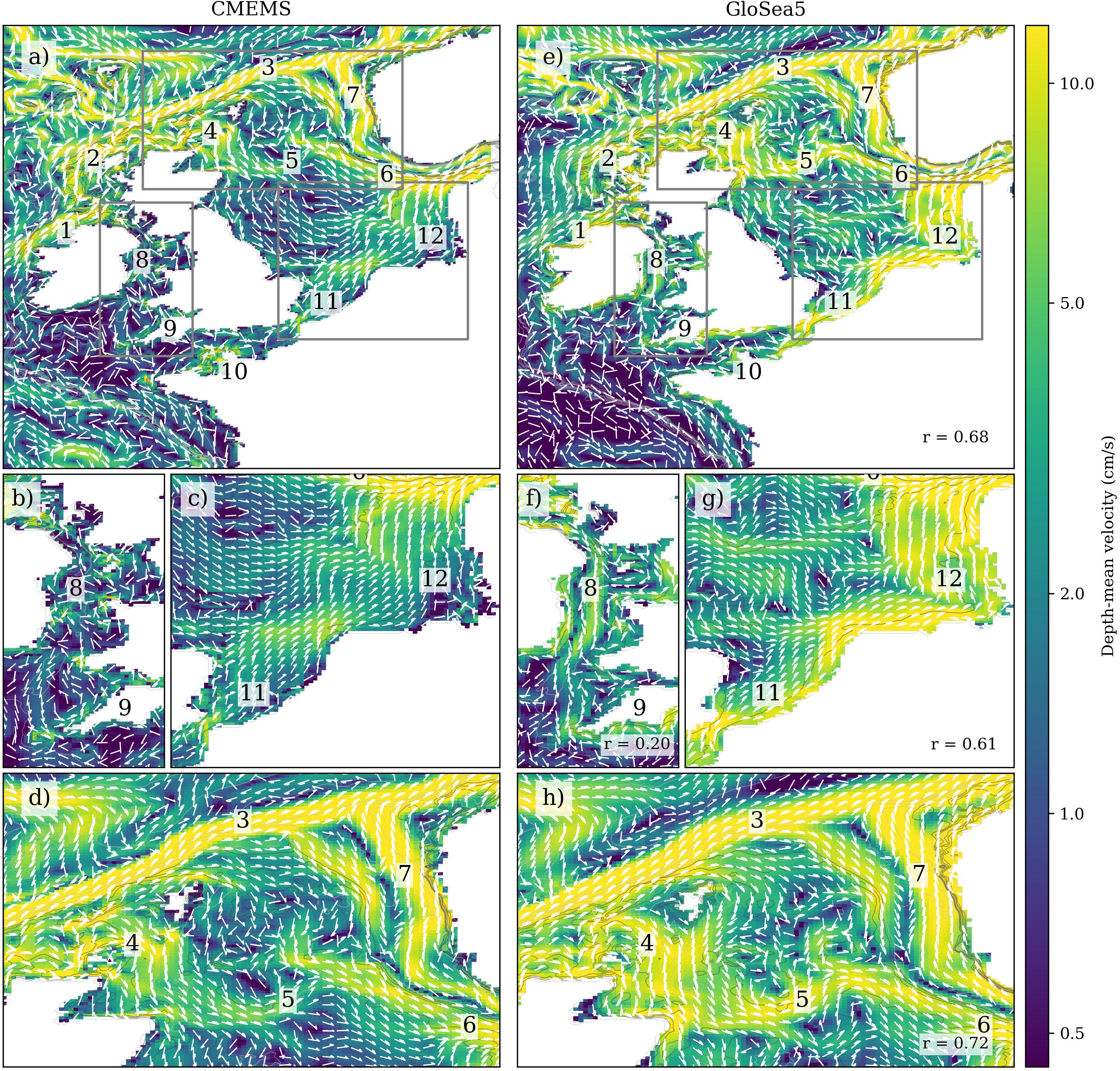
Figure 2. Circulation of CMEMS (a–d) and GloSea5 winter depth-mean climatology (e–h). The arrows show the direction of the currents, and the colouring shows the current magnitude (cm/s, note the colouring on a logarithmic scale). An overview of the NWS circulation is given in panel (a,e). Further (zoomed) details of important regions are given in panels (b–d,f–h), which correspond to the grey boxes in the upper panels (a,e). The spatial correlation of the depth mean current magnitude between each pair of panels is given in (e–h). This is only calculated from grid boxes within each panel, that are within the NWS. The equivalent plots showing salinity (and temperature) distribution for the average of 2010/2011 and 2011/2012 are given in Supplementary Figures 5, 6, to show the relationship between advection and tracer distribution. Figure 8 compares the depth mean circulation of CMEMS and CO6 averaged over the 2010/2011 and 2011/2012 winters. Relevant NWS circulation features are numbered and described in Box 1.
Many of the main features of the residual NWS circulation are captured by GloSea5 (see the Box 1 for retails): there is a shelf slope current flowing from the west of Ireland (numbered 1 on Figure 2), around Scotland (Figure 2(2)) and past the Shetlands, and extending towards Norway (Figure 2(3)); the North Sea inflow either side of the Orkneys (Figure 2(4)) continuing as the Dooley Current (Figure 2(5)), and then flowing south-east into the Skagerrak (Figure 2(6)); the outflow in the eastern Norwegian Trench (Figure 2(7)); and the general cyclonic (anti-clockwise) circulation in the North Sea – these are all represented, and lead to a spatial correlation of r = 0.68 (between the CMEMS and GloSea5 NWS depth mean current magnitudes).
BOX 1. Pertinent features of the CMEMS and GloSea5 NWS circulation, as shown in Figure 2. NWS circulation features that are relevent to this study are are numbered in the panels of Figure 2: The shelf slope current (1, 2, 3) follows the shelf break (∼500 m isobath). Inshore of this, (1) The Irish Coastal Current links to the Scottish Coastal Current, and then (4) the northern North Sea inflow; (5) and the Dooley Current (following the 100 m isobath) connects to the (6) inflow into the Skaggerak, which retroflects, and flows out as (7) the Norwegian Coastal Current. GloSea5 has an incorrect southward flow through the Irish Sea (8, in subpanel f), which continues along the northern (English) coast of the English Channel (9) – in CMEMS the stronger western Engish Channel currents are along the French Coast, and around the Channel Isles (10), asssociated with substantial tides. The English Channel North Sea Inflow follows a different pathway through the Southern Bight (11) and the German Bight (12) in GloSea5 and CMEMS, with the CMEMS flow mainly to the west of 11 and 12 (c), and the GloSea5 flow to the east of 11 and 12 (g).
The currents in GloSea5 tend to have a greater magnitude than in CMEMS, particularly in the Northern North Sea (Figures 2d,h), English Channel (Figures 2a,e), Irish Sea (Figures 2b,f), and the southern North Sea (Figures 2c,g). There are several regions where the configuration of the currents is notably different: the English Channel (Figures 2(9,10)); the Southern Bight (the main current is west of 11 in Figure 2c, and east in Figure 2g); the German Bight (the main current is west of 12 in Figure 2c and east in Figure 2g); the Irish Sea (Figure 2(8)); and the to the west of Scotland. Off the shelf, the depth mean currents are much weaker over large areas in GloSea5 (i.e., in the Bay of Biscay). In the Irish Sea, GloSea5 has a strong northward coastal current that flows along the Irish coast, until Newcastle in Northern Ireland – this is absent in CMEMS. In GloSea5, there is a southward current through the North Channel that extends down to Cornwall (Figure 2(8)), where it flows eastward, along the northern (English) coast of the English Channel (Figure 2(9)). This is a substantial error in the GloSea5 circulation, as CMEMS has a northward flow, and is reflected in the local spatial correlation of r = 0.2 (Figure 2f). The estimated volume transport (described, with its limitations, in the Appendices) through the Irish Sea (Supplementary Figures 1, 4) suggests that GloSea5 ensemble mean has a (temporal) mean net southward transport of 0.12 Sv ± 0.05 (mean ± 1 standard deviation), with a southward flow every year, while CMEMS has a northward flow of 0.05 Sv ± 0.07, and a northward flow on 20 of the 23 years. There is also a cyclonic recirculation cell to the east of the Isle of Man in GloSea5. All of this is absent in CMEMS, and as far as is known, reality. In the English Channel GloSea5 also has a strong north-eastward current flowing along the French coast from Le Havre through the Dover Strait, and along the European coast into German Bight. This current structure is absent from CMEMS. CMEMS has stronger currents to the west of Normandy (around the Channel Islands, Figure 2a(10)) - this is a region of strong tides which can impact on the residual currents. In CMEMS there is perhaps an intensification of the current through the Dover Strait, but this is much weaker to the east and west, compared to GloSea5. When comparing the volume transport estimates (Supplementary Figure 4), there is a greater flow through the Dover strait in GloSea5 (0.14 Sv ± 0.04 Sv), but weaker interannual variability in the GloSea5 ensemble mean (cf. CMEMS = 0.09 Sv ± 0.06 Sv). In the southern North Sea, the substantial GloSea5 current follows the coast (Figure 2g(11)), whereas in CMEMS, it remains in deeper water (typically deeper than 25 m). As the current flow towards the Skagerrak, it bypasses the shallow German Bight in CMEMS (Figure 2c(12)), whereas it still follows the coast in GloSea5. To the north of Northern Ireland and west of Scotland, the GloSea5 Irish Coastal Current is further onshore than in CMEMS (Figure 2(1)), and so part of it then follows the coast southwards into the Irish Sea. The other part forms the Scottish Coast Current, which tends to follow the coast closely, even flowing southwards around the northern side of Isle of Skye. In CMEMS, the Irish Coast Current is further offshore, does not turn south into the Irish Sea, follows the Scottish coast further offshore, tending to flow outside the Hebrides. The northern North Sea inflow appear stronger in GloSea5 than in CMEMS (Figure 2(4)), but the volume transport estimates (Supplementary Figure 1) suggest similar mean values (GloSea5 = 0.73 Sv ± 0.07 Sv, CMEMS = 0.75 Sv ± 0.15 Sv). The northern North Sea inflow seems to have less impact on the temperature and salinity predictability of the system [when compared to the southern (English Channel) North Sea inflow]. These circulation pathways help explain the difference in salinity (and temperature) patterns between CMEMS and GloSea5 (see Supplementary Figure 5). The saline (and warm) plume flowing from the Dover Straits into the southern North Sea in CMEMS (Figures 1a,d,g) follows the CMEMS current pathway. The tighter band of low salinity CMEMS water along the European coast is within the 25 m isobath, where the currents are much slower. This perhaps allows the lower observed salinity of the CMEMS in this area – in GloSea5 the stronger current following the coast would flush these regions of freshwater influence to a greater extent.
We also compare the GloSea5 winter SST and SSS climatology to different observation products (Supplementary Figure 7). Given the limitations of evaluating against EN4 and CMSA, and the redundancy of evaluating against OSTIA, we have not included this analysis the main body of the paper, but include the figures in the Supplementary Materials for completeness, and describe the datasets in the Appendices. GloSea5 SST minus OSTIA shows the same SST bias pattern and values as Figure 1c – this is expected as CMEMS assimilates satellite SST observations. The EN4 SSTs are lower than OSTIA and CMEMS, but seem to corroborate GloSea5 being too cold in the English Channel, the south eastern North Sea, west of Scotland, and the Irish Sea. The GloSea5 minus EN4 SSS is in good agreement with Figure 1f, showing GloSea5 to be too salty around Scotland, and too fresh in the Irish Sea, English Channel and southern North Sea. The GloSea5 SSS minus CMSA SSS is difficult to use as the analysis error is larger than the bias (Supplementary Figure 2). The CMSA SSS is too fresh in the North Sea (compared to the CMEMS and EN4), and so the GloSea5 CMSA biases are too salty here. It is interesting to note that the CMSA also suggests that GloSea5 is too fresh in the Irish Sea, English Channel and in the Southern Bight.
We now look at how well the GloSea5 forecast system captures the climatological seasonal evolution through winter and spring (Figure 3 and Supplementary Figure 8). For each of the validation regions, we have calculated the monthly means from November to May of the following year for every year from CMEMS (and these are given as the faint black lines in Figure 3), and these are averaged into the climatological mean (in the bold black line). The GloSea5 ensemble mean forecasts for each year (given as the faint red lines) are also averaged into the climatological mean (bold red line). These are all anomalies, so the mean of the climatology has been removed from each year (i.e., the bold lines average to zero).
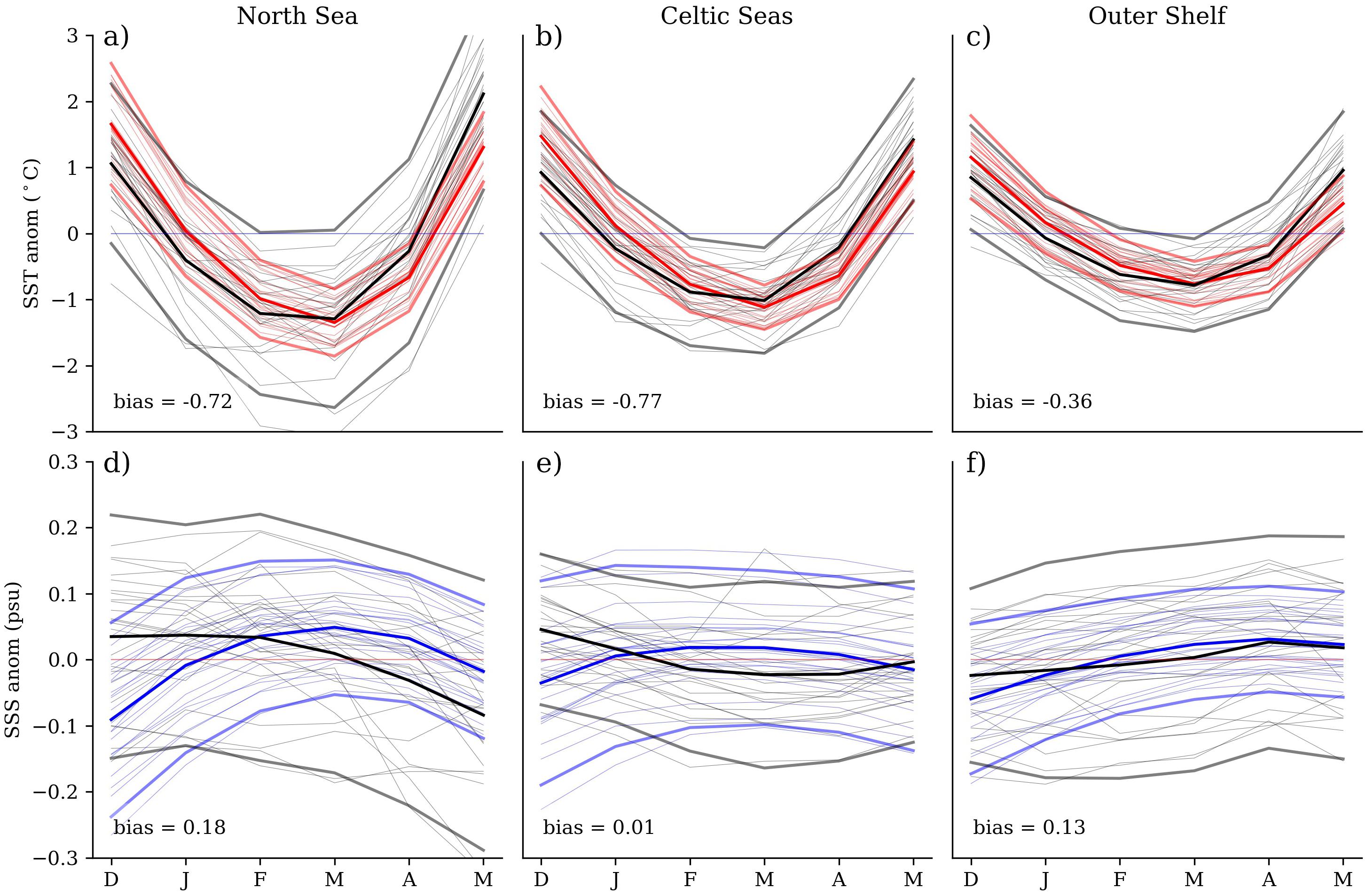
Figure 3. The regional mean seasonal evolution of SST (a–c) and SSS (d–f) for 3 regions [North Sea (a,d), Celtic Seas (b,e), and Outer Shelf region (c,f) - the regions are defined in Figure 1a], for CMEMS (black) and GloSea5 ensemble means (temperature red, salinity blue). For CMEMS, each year (between 1993 and 2016) is given as a thin line, with the climatological mean year as a bold line. Interannual spread for CMEMS and GloSea5 is given with ± 1.96 standard devations. The mean bias is given in each panel. NBT is given in Supplementary Figure 8.
The temperatures have temporal correlations >0.9 (although as there are only 6 monthly means, we do not consider the significance) suggesting CMEMS and GloSea5 have similar climatological temperature evolution through winter (Figures 3a–c). They have relative standard deviations (RSD) near unity suggesting a similar inter-annual variability, but there is a <1°C negative bias (GloSea5 is too cold compared to CMEMS). There are differences in the seasonal evolution of SSS, however as the seasonal cycle is weak compared to interannal variability (in both CMEMS and the GloSea5 reforecasts), these differences are not significant (Figures 3d–f). There is similar interannual varibility in CMEMS and in GloSea5, although GloSea5 is greater in the Celtic Seas.
Overall, we find that GloSea5 captures the climate of the NWS winter relatively well. The NWS winter surface and bed temperature are well represented by GloSea5 when the NWS is well mixed, and the temperatures are driven by surface heat exchange, which tends to occur at a relatively large spatial scale. The overall salinity pattern is fairly well represented, although local details are sometimes missed. The salinity pattern is less controlled by atmospheric processes than temperature, with circulation and rivers dominating – neither of which are particularly well represented in the GloSea5 system (e.g., GloSea5 river mouths are mapped offshore of the model grid coastline, Walters et al., 2017; Supplementary Figure 11g).
How Well Does GloSea5 Predict Winter Conditions on the NWS?
We have shown that GloSea5 simulates the mean climate state of the NWS and the broad pattern of circulation. We have seen that there are important details of the circulation that are incorrect, which can lead to errors in the salinity and, to lesser extent, temperature fields.
We now assess how well GloSea5 predicts the year-to-year variations in winter conditions on the NWS. We also consider how the GloSea5 predictability compares to persistence. Initially we compare regional means (as defined in Figure 1a) of the GloSea5 DJF (as forecast in November) with those from CMEMS (Figure 4 and Supplementary Figure 9), but then examine the spatial patterns of the differences (Figure 5 and Supplementary Figure 10).
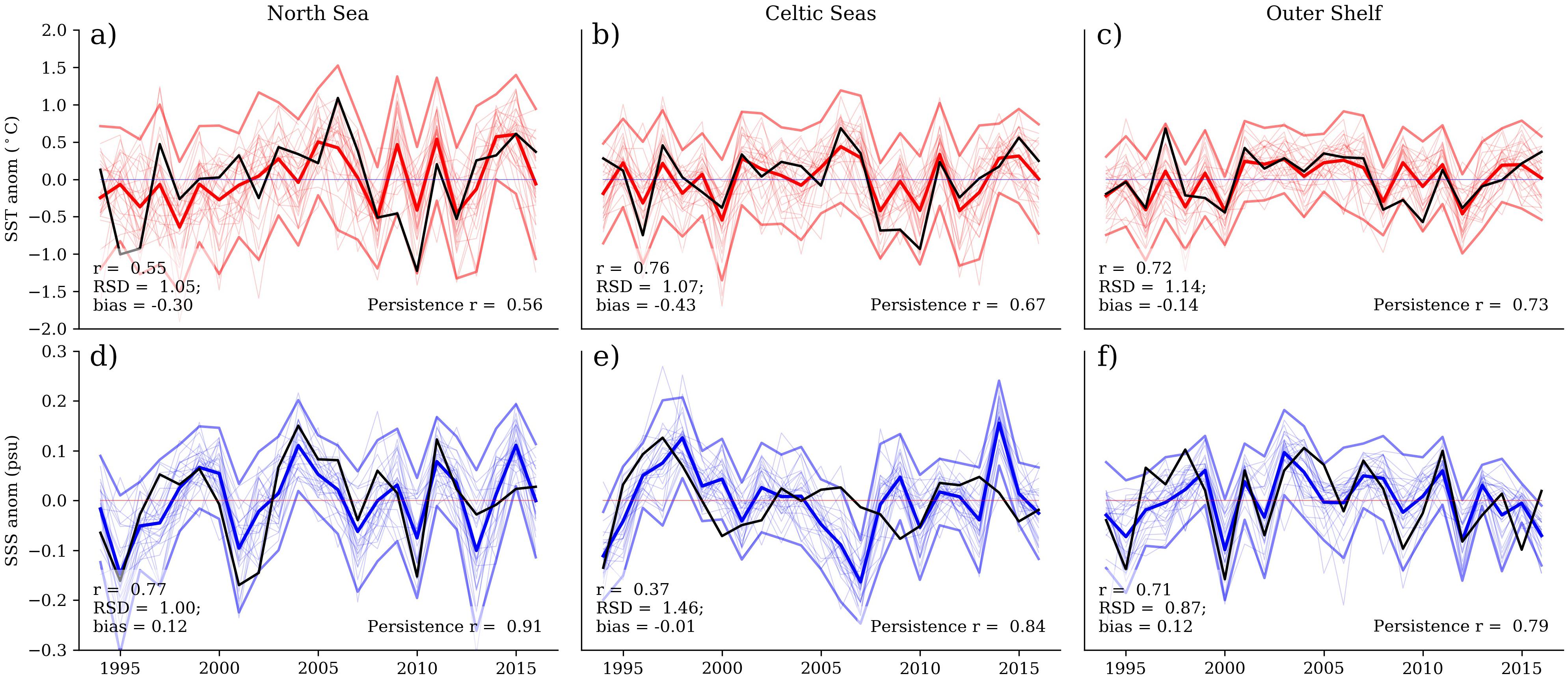
Figure 4. Assessment of GloSea5 predictability of the NWS winter for SST (a–c) and SSS (d–f). The DJF mean (from each year) is averaged over the validation regions (defined in Figure 1a). CMEMS is in black. GloSea5 reforecasts (DJF mean predicted from November) are coloured (temperature: red; salinity: blue). Each of the 28-ensemble member is shown as a faint line, and the ensemble mean, and ±1.96 ensemble standard deviation is shown in bold coloured lines. These are presented as anomalies of the temporal mean of the time series (ensemble mean for the GloSea5 data). The correlation skill (r), relative standard deviation (RSD, taking the variability of the ensemble into account), bias and (Eulerian) persistence skill is given for each panel. NBT is given in Supplementary Figure 9.
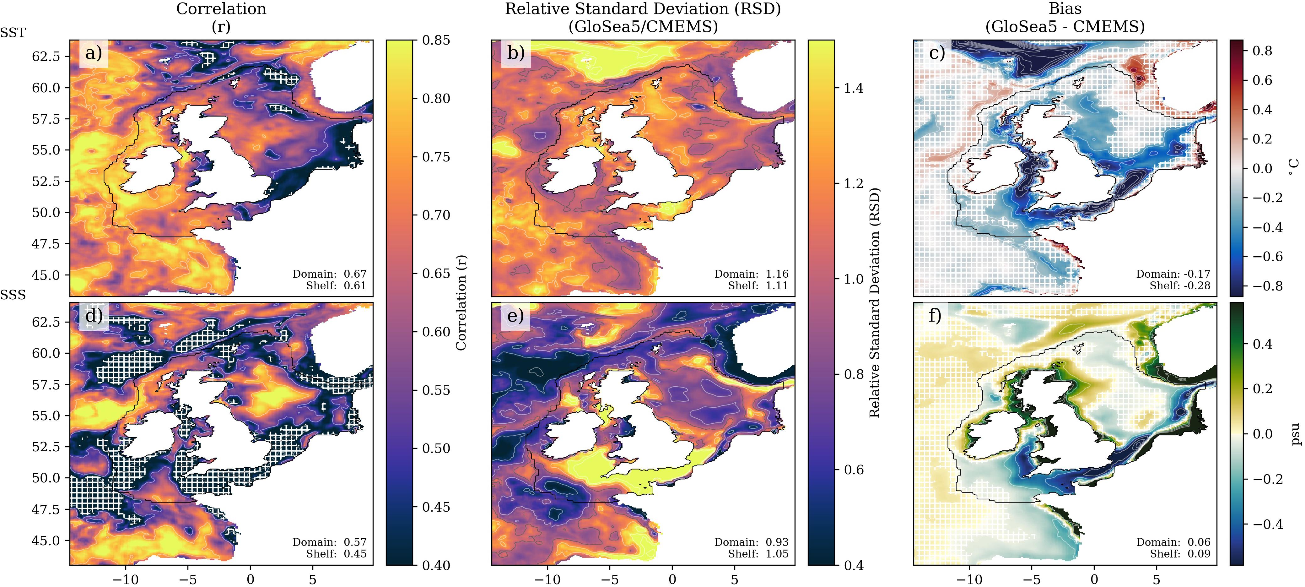
Figure 5. Assessment of GloSea5 forecast skill of the NWS winter for SST (a–c) and SSS (d–f). The winter (DJF) mean CMEMS is compared to GloSea5 reforecast ensemble mean (DJF predicted from November). The (pointwise) statistics compare the pair of 23-year time-series, giving (a,d): the correlation (with insignificant values shaded out); (b,e): relative standard deviation (RSD, the standard deviation of the GloSea5 ensemble member time-series (23 years and 28 ensemble members) divided by the standard deviation of CMEMS time-series); and (c,f): the bias (repeated from Figures 1c,f for ease of comparison). The domain and shelf mean are given for each field. NBT is given in Supplementary Figure 10.
We find GloSea5 ensemble mean temperature has good correlations with CMEMS in the Celtic seas (Figure 3b, the region including the Celtic and Irish Seas and the English Channel, blue in Figure 1) and the Outer shelf region (r ≈ 0.7, Figure 3c, green in Figure 1) while slightly lower in the North Sea region (r = 0.55, Figure 3a, red in Figure 1). The associated RSD is about RSD ≈ 1.05, reflecting similar inter-annual variability to CMEMS (Figure 4). Salinity has relatively good correlations in the North Sea and outer shelf region with r > 0.7 (Figures 1d,f). In the Celtic Seas (Figure 4f), there is a lower correlation (r ≈ 0.37, reflecting a period from 2004 to 2010) and much higher RSD (RSD = 1.46 c.f. RSD ≈ 1 in most other regions). This is one of the regions where the circulation is very different. This is the only variable and region (in Figure 4) where the GloSea5 inter-annual variability is much greater than that of CMEMS (i.e., RSD > 1.2).
These regional means give an overview and allow the temporal evolution to be examined. We now examine the spatial patterns of agreement between GloSea5 and CMEMS with point wise statistics (Figure 5) – these help to show where GloSea5 has prediction skill.
SST is significantly correlated across the domain (Figure 5a) – this correlation is a measure of the deterministic skill. Correlations are high to the west of the United Kingdom (r > 0.7), moderate over most of the North Sea, but low in the southern part of the North Sea. There is also a region of lower deterministic skill in the north-eastern North Sea (between the Dooley Current, and the northern shelf break) – this region is collocated with a region where the GloSea5 current magnitudes are much greater than in CMEMS. NBT correlations are similar to SST on the shelf, greater in the southern part of the Norwegian Trench, but are largely uncorrelated in the open ocean (Supplementary Figure 10). The SST and NBT RSD ≈ 1.1 across the shelf (Figure 5b), again reflecting the similar interannual variability between GloSea5 and CMEMS. There is a slight cold temperature bias (-0.28°C when averaged across the shelf), which is greatest in the Irish Sea, English Channel, and southern North Sea (<-0.5°C) (Figure 5c).
Interannual salinity variability can be affected by advection, local river input, and the local precipitation minus evaporation (assumed to have a negligible at these local scales). However, local (regional and ensemble mean) GloSea5 salinity is only weakly correlated with the GloSea5 rivers, suggesting that river variability plays only a secondary role in the winter interannual salinity variability of the GloSea5 NWS (Supplementary Figure 11g). The correlation patterns between regional salinity and estimate of transport (Supplementary Figures 11a,c,e) are coherent and suggest advection is an important driver of NWS interannual winter salinity variability.
Much of the NWS SSS has low or insignificant temporal correlation (between the GloSea5 ensemble mean and CMEMS, Figure 5d). There are strong correlations between GloSea5 and CMEMS salinity in the Irish Shelf region, and parts of the western central North Sea, both regions where the salinity is mainly controlled by ocean processes. Conversely, the English Channel, Irish Sea and southern North Sea (regions with important riverine forcings, strong tidal currents, and large differences in the modelled circulation) are generally uncorrelated. The difference in the strength of the circulation to the north of the North Sea, and the northern North Sea inflow may explain the low salinity correlations in the northern North Sea. The low SSS correlation in the NT and Skagerrak/Kattegat are unsurprising given the different treatment of the exchange with the Baltic Sea, and the complexity of this region. The SSS RSD panel show values of 0.8-1.4 for most of the shelf (Figure 5e), apart from a region (with low correlation) extending from the Celtic Sea through the English Channel and into the southern North Sea, where GloSea5 has much greater SSS interannual variability than CMEMS. This region is also much fresher in GloSea5 than in CMEMS (Figure 5f). If GloSea5 does not represent this circulation pathway properly (as suggested in Figures 1, 2), rather than higher salinity water from the Celtic Sea being transported through the English Channel into the southern North Sea, there could be a greater proportion of fresher water from the Irish Sea. This is supported by the correlation between the GloSea5 Irish Sea transport and salinity in the Irish shelf and the Celtic Sea and English Channel (Supplementary Figures 11a,c). Years that have stronger (southward directed) GloSea5 ensemble mean Irish Sea transport also have fresher Celtic Sea and English Channel (with correlations of 0.54 and 0.33 respectively), while years where the transport is weaker have a fresher Irish shelf region (north west of Ireland and Scotland; correlation of -0.56). This supports our proposed GloSea5 advective pathway from the Irish Sea to the southern North Sea. The English Channel transport and SSS correlations show local salinities (Celtic Sea, English Channel, and southern North Sea) are higher when the eastward directed flow is stronger (correlations 0.29, 0.51 and 0.43 respectively), reflecting a separate advective pathway of Atlantic water from the Atlantic to the southern North Sea bringing higher salinity water into the southern North Sea. The GloSea5 SSS has a slight negative bias (0.09) when averaged over the shelf, but this reflects a region of positive bias (>0.3) around Scotland and the northern and western side of Ireland (perhaps reflecting the greater GloSea5 North Sea inflow), and a region of negative (<-0.3) bias in the Irish Sea, Celtic Sea, English Channel and Southern North Sea.
How Much Inherent Persistence Is There on the NWS? Does GloSea5 Deterministic Skill Beat This Persistence?
We now consider whether there is inherent persistence of winter conditions on the NWS (Figure 6). Most of the domain has SST persistence between 0.6 > r > 0.7, with a domain mean of r = 0.68 (0.40 – 0.80 at the 5th – 95th percentiles). The NWS mean SST Eulerian persistence is r = 0.62, and is lower in southern and eastern North Sea, particularly in the Southern Bight (Figure 6b). There is also a region in the north-eastern North Sea (between the Shetlands and the Norwegian Trench, north of the Dooley Current) where the SST persistence is lower – this could be related to circulation variability. Surface salinity has a similar domain mean Eulerian persistence to SST (r = 0.66) but with a greater range of values (0.27 – 0.89 at the 5th – 95th percentiles, Figure 6e). On the NWS the SSS persistence is lower (r = 0.59). The NWS has low SSS persistence in the southern North Sea, north of the Dooley Current, in the Celtic Sea and around Ireland and Scotland. These regions have large residual flows or large riverine inputs. Conversely, in the centre of the North Sea, Irish Sea, and northern (and western) English Channel, regions with lower mean residual velocities or no large rivers, there is greater persistence.
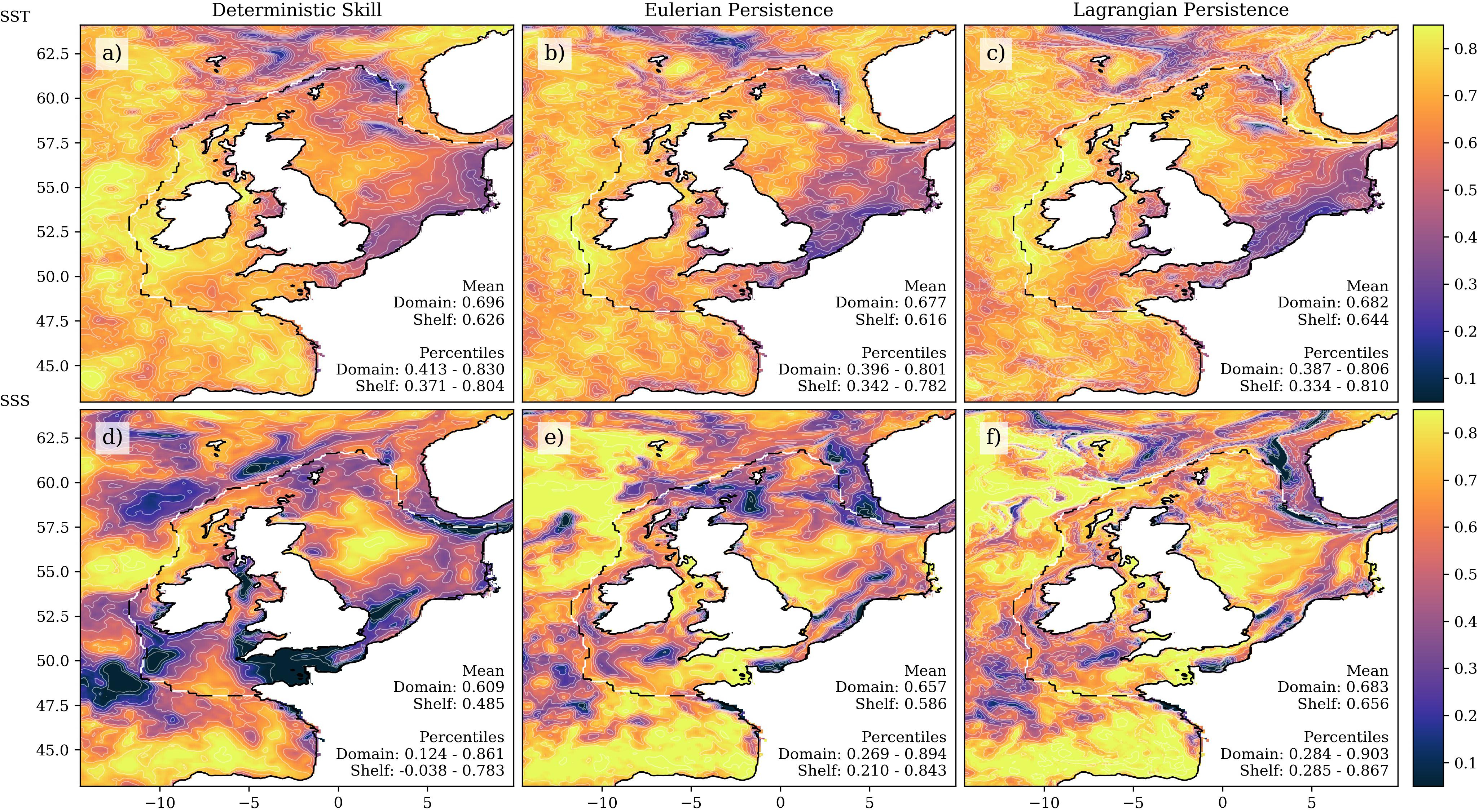
Figure 6. Deterministic skill (a,d) and Persistence [Eulerian (b,e) and Lagrangian (c,f)] for SST (a–c) and SSS (d–f). The black and white dashed line delineates the NWS shelf region. Spatial statistics, including the mean value, and the range of values at the 5th and 95th percentiles, are given in each panel.
In many regions of the NWS (50%, Table 1), the SST persistence is close to the deterministic skill (Figures 6a, 7a,b) and so the deterministic skill is not significantly different from persistence (hatched areas in Figures 7a,b, when tested with the bootstrapping technique described in the Methodology section). To the west of the United Kingdom and in the southern and central North Sea, the deterministic skill is greater than persistence (r ≈ 0.1, Figure 7), and there are small regions where this is significant. North of the Dooley Current, in the Norwegian Trench and against the Jutland Peninsula, the deterministic skill is significantly less than persistence by a similar magnitude. This reflects the lower deterministic skill in this region. Overall, SST deterministic skill significantly greater than persistence over 25% of the NWS and is significantly less over 24% of the NWS (Table 1).
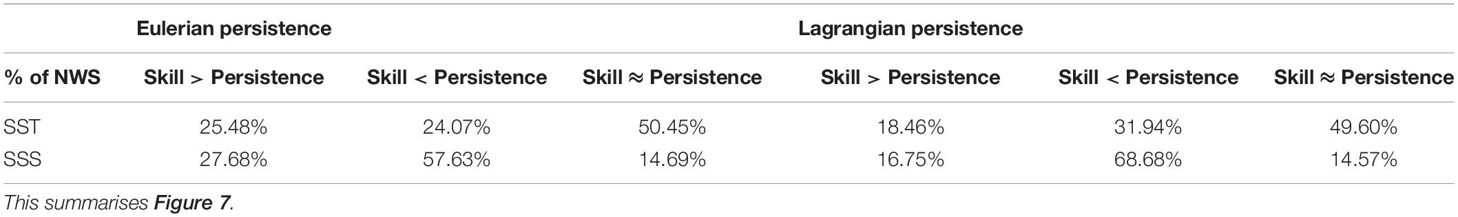
Table 1. Proportion of the NWS where the deterministic skill is significantly greater or less than persistence, and where there is no significant difference, for Eulerian and Lagrangian persistence, for SST and SSS.
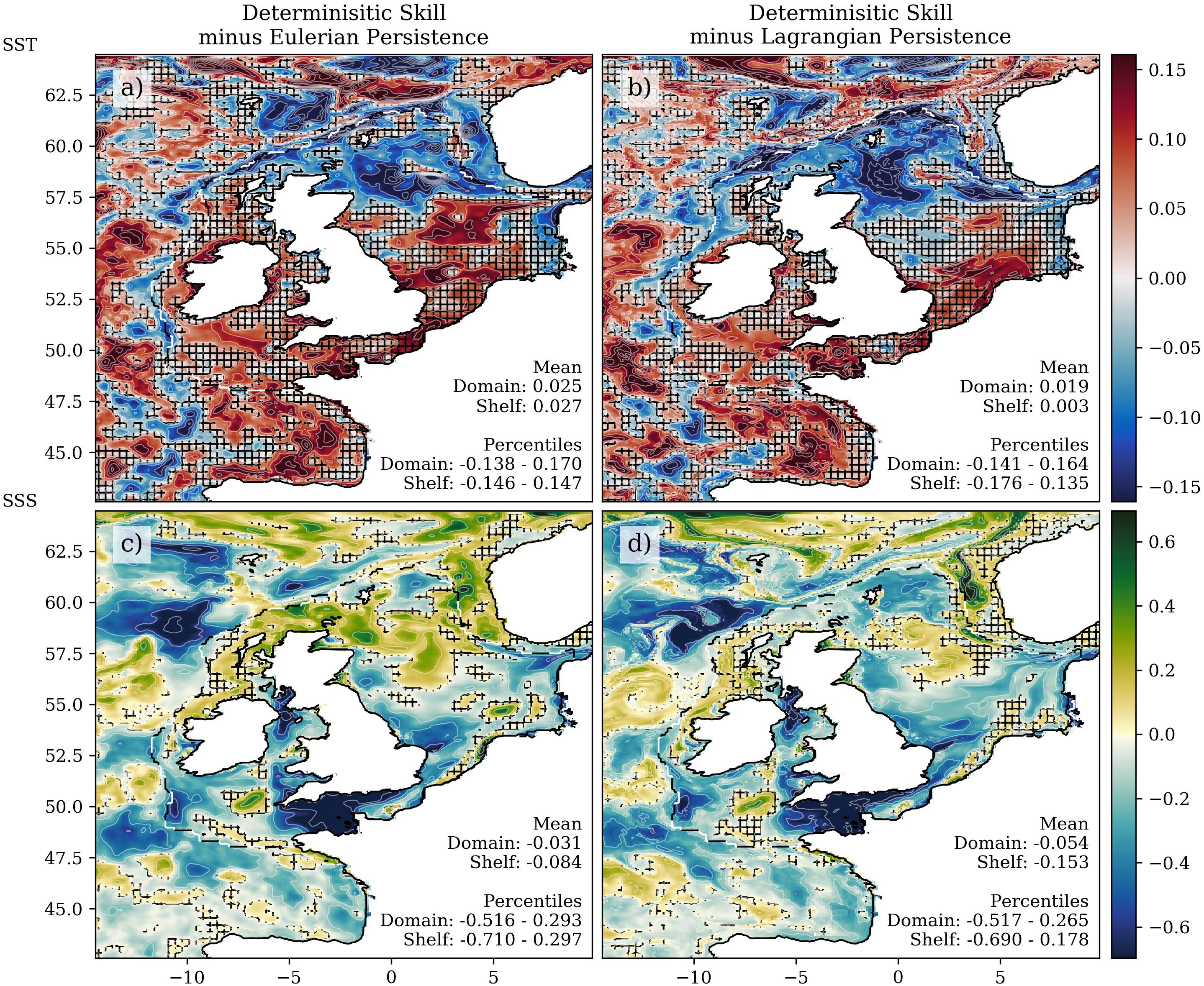
Figure 7. Deterministic skill minus (Eulerian and Lagrangian) persistence for SST (a,b) and SSS (c,d) (Eulerian a,c, and Lagrangian b,d). Insignificant differences are marked with hatching. The proportion of the NWS where the skill is significantly greater or less than persistence is tabulated in Table 1. Spatial statistics, including the mean value, and the range of values at the 5th and 95th percentiles, are given in each panel.
The NWS SSS deterministic skill is generally significantly less than persistence (over 58% of the NWS, Table 1), particularly in the southern North Sea, English Channel, Irish and Celtic Seas, being about r ≈ 0.3 less than persistence (Figures 6d–f, 7c,d). In contrast, NWS SSS deterministic skill is significantly greater than persistence (by about r ≈ 0.3) along the route of the North Sea inflow and continuing along the Dooley Current. However, when looking at the deterministic skill and persistence maps (Figure 6), it is clear that this region has low deterministic skill in GloSea5 and low persistence in the observations. This is an important transport pathway, and we have shown that the GloSea5 residual circulation is too strong (Figures 2d,h although has the correct spatial configuration). GloSea5 is likely to advect salinity anomalies too rapidly which will reduce deterministic skill, as will any incorrect variability introduced from Scottish (and Irish) rivers. Even if the skill exceeds persistence in this region, it is still low.
Given the role of advection (particularly in the northern North Sea region), comparing the salinity in the same grid box months apart (i.e., Eulerian persistence being calculated by correlating the November values with the winter mean values grid box by grid box) may not be the most appropriate measure of NWS persistence. In addition to the Eulerian persistence described above, we have also considered the Lagrangian Persistence (as described in the Methodology section, Figures 6c,f). There is a marked increase in the SSS persistence (from the Eulerian to Lagrangian) throughout the northern NWS, particularly in the North Sea inflow region (north of Scotland, though the North Sea inflow between the Scottish mainland and the Shetland, along the Dooley Current, and to the north of the Dooley Current). There is also an improvement in the persistence in the southern North Sea. The persistence increases in the Dover Strait and East Anglian Plume, although there is a region between them where the more variable flow leads to lower persistence. The increased persistence (when changing from Eulerian to Lagrangian persistence) in the northern North Sea means that GloSea5 SSS deterministic skill is no greater than (Lagrangian) persistence along the path of the North Sea inflow (north and east of Scotland). The proportion of the NWS where the SSS deterministic skill is significantly greater than persistence decreases from 28% to 17% when changing from Eulerian to Lagrangian persistence, and the proportion of the NWS where SSS deterministic skill is significantly worse than persistence increases from 58% to 67% (Table 1).
Changing from Eulerian to Lagrangian persistence has less impact on the assessment of GloSea5 SST than SSS. There is a small increase in SST persistence across most of the northern part of the NWS (west of Ireland, and Scotland, most of the North Sea apart the Southern to German Bight regions), but this is typically less than r < 0.1. This leads to a decrease in the area of the NWS where SST skill is significantly greater than persistence from 25% to 18%. There is little change in the regions where the deterministic skill is significantly greater than persistence (compare the hatched regions on Figures 7a,b), although the regions in the central North Sea (where the deterministic skill is significantly greater than persistence) reduce. This reflects the greater importance of surface forcing compared to advective processes for temperature than salinity.
Is GloSea5 Fit for the Purpose of NWS Seasonal Prediction?
GloSea5 has significant skill at predicting winter NAO, the leading mode of climate variability for northern Europe. It also successful at simulating the NWS temperature seasonal cycle, and the spatial patterns of SST, NBT, and SSS. Absolute SST and NBT biases are <1°C over most of the NWS and are insignificant in many regions. The GloSea5 (absolute) salinity biases are larger and are significant over a greater portion of the NWS but are still generally < 1 psu. Errors in the GloSea5 NWS circulation, are likely to be responsible for many of these the significant biases (the Irish Sea, English Channel, southern North Sea for temperature and salinity, and around Scotland for salinity) and are likely to reduce the deterministic skill in these regions. The GloSea5 deterministic skill is not much better than persistence in most places.
We consider GloSea5 fit for purpose for winter NWS seasonal predictability of some variables in some locations. For example, SST and SSS along the northern North Sea inflow pathway (from the west and north of Ireland, around Scotland (south west of Shetland), and into the north-western North Sea) have good deterministic skill (Figures 5a,d) and high persistence (Figures 6b,c,e,f) although have significant biases (Figures 1c,f). Furthermore, SST in the Celtic Sea, western English Channel and Irish Sea also has good deterministic skill and high persistence, however due to incorrect circulation (Figure 2, marked locations (8-10)), errors in the climatological SST field (Figures 1a,b) and significant biases (Figure 1c) in this region, care must be taken. We will show that it is fit for the purpose of providing boundary conditions for downscaling.
We note that there are important differences in the mean winter circulation, when the NWS is fully mixed. In the summer there are seasonal stratified and well mixed regions, separated by tidal mixing fronts, which drive important baroclinic currents. GloSea5 is unable to simulate these finer scale features (Tinker et al., 2018), and so the direct use of GloSea5 for non-winter seasonal predictions is less promising.
How Does Dynamical Downscaling Affect Predictability?
We have looked at how well GloSea5 reproduces the NWS winter climatology, the seasonal evolution, and how well it predicts the NWS winter conditions. Although there are many parts of the NWS where the winter conditions are captured by GloSea5, we have also highlighted some important aspects that are not captured well. We now evaluate how dynamical downscaling affects the performance of the predictions.
Dynamical downscaling is computationally expensive, so here we use a case study, comparing two winters with opposing conditions and NAO states. This simplification prevents us from assessing the deterministic skill of the downscaling system. It also prevents us from producing a CO6 climatology or anomalies for the individual years. However, the difference between 2 years is independent of any climatology, so our case study focusses on detecting this difference. Our results are in part dependent on how different the two winters are (we have shown that they are sufficiently different for temperature and salinity). However, by assessing differences between GloSea5 and CO6 downscaling, we can infer if downscaling leads to improvements in simulating the NWS.
We initially note that the downscaled CO6 mean winter circulation (Figure 8) is much improved from GloSea5 (when compared to CMEMS), with an increase in the NWS current magnitude spatial correlation from r = 0.68 in GloSea5 (Figure 2e, 1992-2018) to r = 0.81 in CO6 (Figure 8e, 2010/2011 and 2011/2012). This also allows an improved representation of local details of the temperature and salinity spatial patterns (Supplementary Figures 5, 6). The circulation pathway from the English Channel, through the Dover Strait, Southern Bight and German Bight, and towards the Skagerrak is well represented (Figures 8a,c,e,g(10-12)), and so the warm and salty plume flowing eastward through the English Channel and into the southern North Sea is much clearer in CO6 than in GloSea5 (Supplementary Figures 5, 6, numbered 11). This significantly increases the southern North Sea SST spatial correlation from r = 0.89 (for GloSea5 and CMEMS) to r = 0.97 (for CO6 and CMEMS), and from r = 0.60 to r > 0.99 for SSS. The pathway from the Shelf Slope Current/Irish Coastal Current/Scottish Coastal Current to North Sea inflow and into Dooley Current structure (Figures 8a,d,e,h (1,2,4,5)) is also improved. The most important circulation improvement is in the Irish Sea, with a local current magnitude spatial correlation of r = 0.83 (Figures 8f,b, c.f. GloSea5 r = 0.20 in Figure 2f). The incorrect southward transport through the Irish Sea is absent in CO6 (Figure 8(8)), this allows the northward warm salty plume through the centre of the Irish Sea (Supplementary Figures 5, 6, numbered 8), with the Irish Sea SST spatial correlation significantly increasing from r = 0.89 in GloSea5 to r = 0.99 in CO6 (when correlated with CMEMS) and r = 0.72 to r = 0.99 for SSS. The south eastward drift across the North Sea that leads towards the Skagerrak is greater in CO6 than in CMEMS, so while the general current structures are correct (in terms of location and direction) there are differences in the magnitudes. This is despite CO6 being forced by the same atmospheric variability as GloSea5. Note that English Channel/southern North Sea and Irish Sea warm salty plumes are averaged out in the difference between years and so not visible in Figure 9 (although can be seen in Supplementary Figures 5, 6).
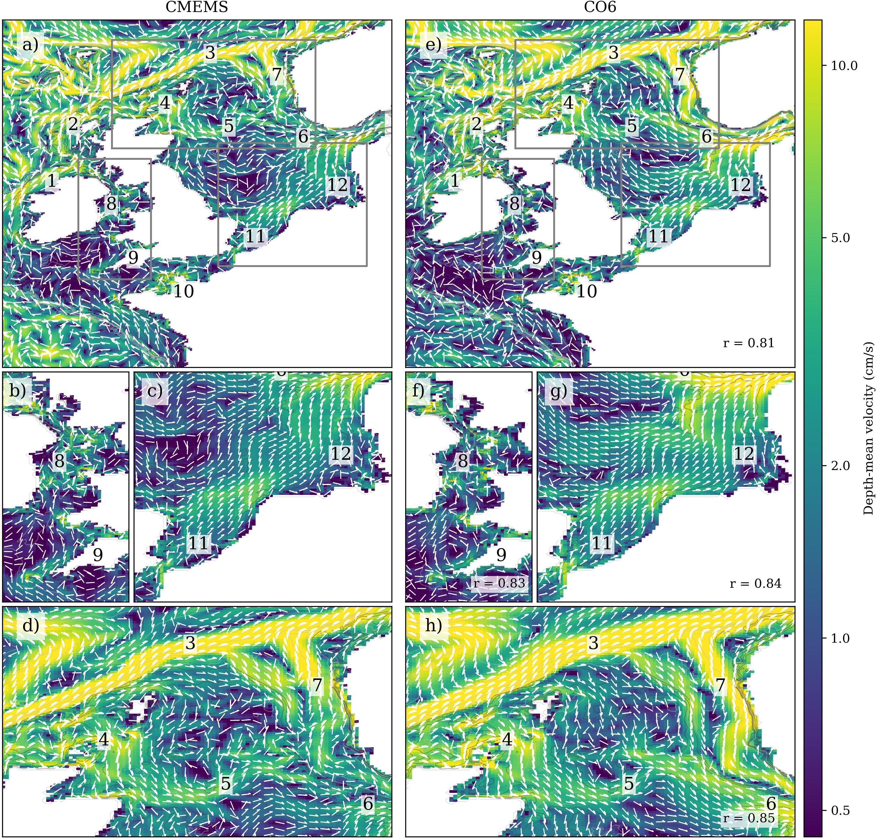
Figure 8. Depth averaged winter mean (2010/2011 and 2011/2012) currents for CMEMS and CO6. See Figure 2 for details, and Box 1 for the numbered circulation features. The spatial correlation of the depth mean current magnitude between each pair of panels is given in (e–h). This is only calculated from grid boxes within each panel, that are within the NWS. Note the CO6 central North Sea circulation (panel e) is close to the CMEMS climatology in Figure 2a.
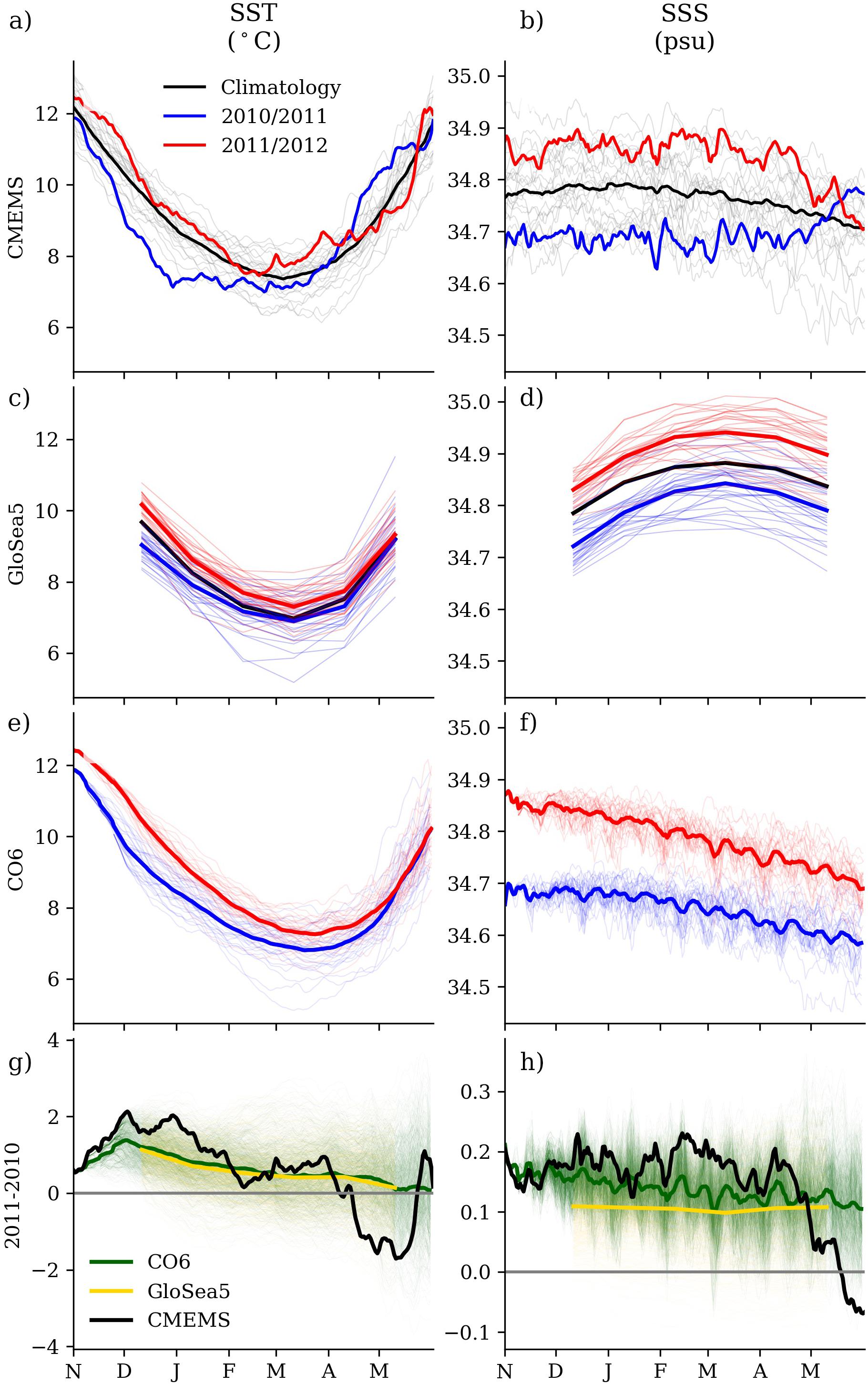
Figure 9. Comparison of the temporal evolution of the 2010/2011 (blue) and 2011/2012 (red) winters for the NWS SST (a,c,e,g) and SSS (b,d,f,h). (a,b): CMEMS: thin black lines, individual years between 1994 and 2016, with the mean year (climatology) shown in bold black. 2010/2011 and 2011/2012 are shown in blue and red respectively. Where a coloured line is above the climatology (bold black), a positive anomaly for that year was “observed.” (c,d): GloSea5 forecasts. Bold black line is model climatology – the average of the ensemble mean forecasts for each year. 2010/2011 and 2011/2012 are shown in blue and red respectively. Thin lines are the individual ensemble member for each forecast year. The bold coloured lines are the ensemble mean GloSea5 forecast. (e,f): CO6 forecasts. Same as for row 2, except there is no climatological seasonal cycle available. The lower row (g,h) is the differences between the years – 2011/2012 - 2010/2011, i.e., how much warmer/saltier/higher 2011/2012 was than 2010/2011. Black line: the difference between CMEMS “observations.” The gold line is the difference between GloSea5 forecasts, and the dark green lines are the difference between the CO6 dynamically downscaled forecasts (ensemble mean in bold and ensemble member pairs as thick lines). Other regions are shown in the Supplementary Materials. NBT is given in Supplementary Figure 12. The legend in (a) applies to (a–d). The legend in (g) applies to (g,h).
Our first assessment of the CO6 simulations focuses on the temporal evolution of the differences between the two winters. There is a general, if (temporally) smooth, agreement for temperature and salinity seasonal evolution between CMEMS and CO6 (and GloSea5) absolute values (Figures 9a–f). The temperature differences (SST and NBT Figure 9g and Supplementary Figure 12c) for CMEMS (black) and CO6 (dark green) agree in sign over the winter period (DJF), although the magnitude is perhaps greater in CMEMS. When looking at the sub-seasonal times scale, the SST difference (Figure 9g) both show an increase though November, then a general decrease. CMEMS has higher frequency variability than the CO6 ensemble mean. Beneath this variability, there appears to be agreement in temporal evolution out to about April. Similar conclusion can be drawn for NBT as SST (Supplementary Figure 12).
The CO6 SSS difference (green in Figure 9h) remains fairly constant with time. There is a general agreement in CMEMS and CO6 SSS throughout the winter. In spring, the CMEMS difference diminishes. There are small oscillations in the CMEMS and CO6 SSS that appear to be correlated. These have a very low amplitude, and reflect the use of the common riverine forcings, rather than having a tidal spring/neap origin (they have appeared to have a 14-day periodicity, but this is not the case). As the CO6 forecasts are initialised from the CMEMS reanalysis, any persistent anomalies are likely to be the same. The comparison between CO6 and GloSea5 show no important differences. This is particularly true for temperature, but also, to a lesser extent for salinity. Similar conclusions can be drawn from the other regions (see Supplementary Figures 15-17).
Important processes and features are not resolved in the relatively coarse ocean of GloSea5, so the temporal evolution of these large regions is only part of the story. The spatial patterns of the difference between years in the CMEMS reanalysis, GloSea5 and CO6 (Figure 10 and Table 2) show the value of downscaling.
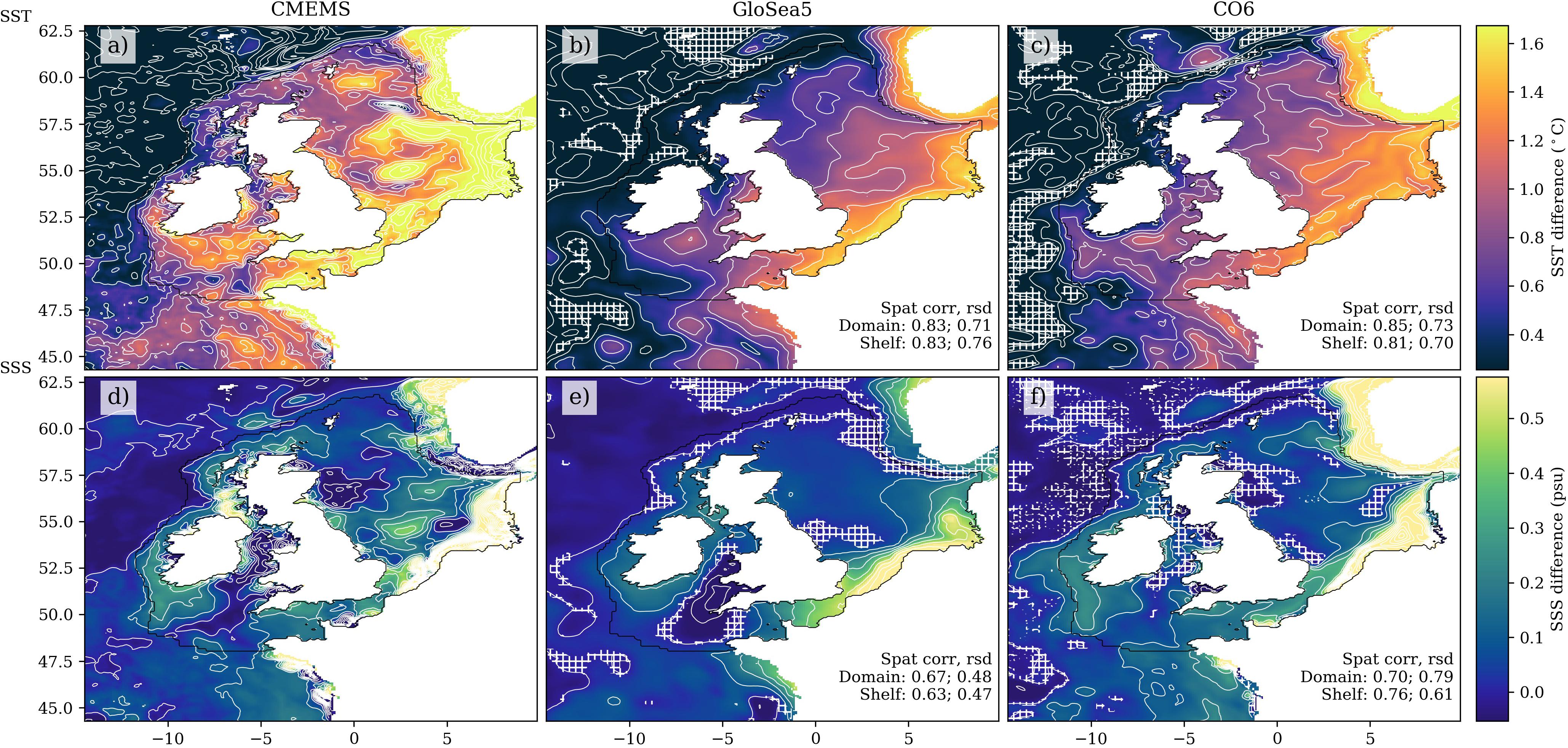
Figure 10. Spatial patterns of the difference of two winter (DJF, 2011/2012 minus 2010/2010) from CMEMS (a,d), GloSea5 (b,e), CO6 (c,f) for SST (a–c) and SSS (d–f). The GloSea5 data has been bilinearly interpolated onto the CO6 grid. White hatching (in panels b–f) shows where there is no statistical difference between the 2011/2012 and 2010/2011 ensemble (using a point-wise Two-tailed Student’s T-Test). The spatial correlation and relative standard deviation, compared to CMEMS, for the full domain, and the shelf region, is given for GloSea5 and CO6 (b,c,e,f). NBT is given in Supplementary Figure 13.
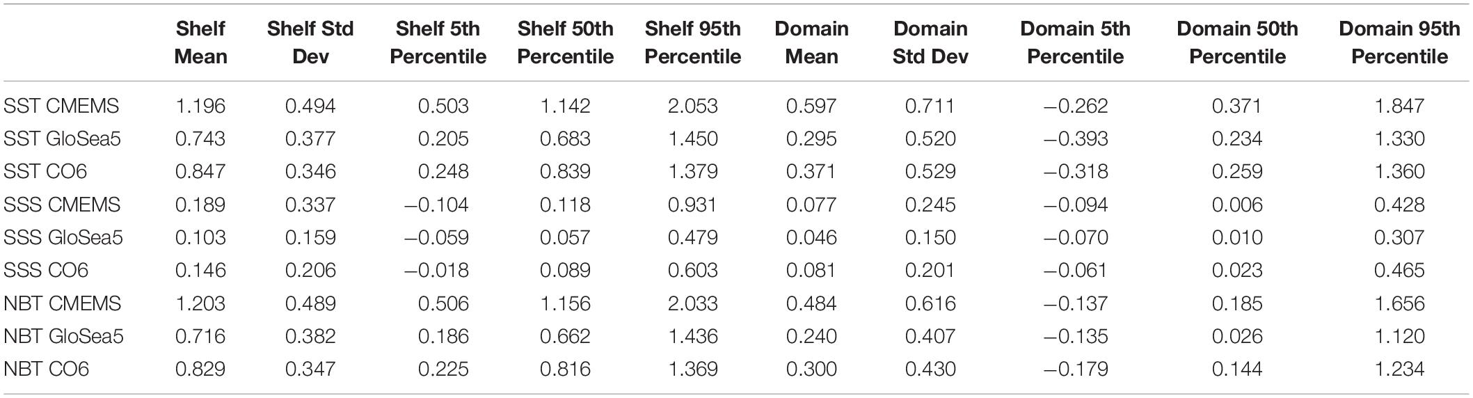
Table 2. Summary spatial statistics of the area mean difference between the two case study years, summarising the values displayed in Figure 10.
GloSea5 reproduces the CMEMS temperature differences between the 2 years well (SST, NBT Figures 10a,b and Supplementary Figure 13), with spatial correlations of >0.8 over the shelf. This reflects the greatest difference between the years in the English Channel, southern and eastern North Sea, with locally warm regions in the northern Celtic Sea, and over the Dogger Bank, and a much smaller difference between the years to the north and west of the United Kingdom and Ireland. There is a significant difference (with pointwise T-tests) between the years across the shelf for both GloSea5 SST and NBT (Figure 10 and Supplementary Figure 13). GloSea5 predicts a smaller difference between the 2 years (0.74°C when averaged over the shelf, ranging from (5th to 95th percentile values) 0.21°C – 1.45°C) than in CMEMS (1.20°C, ranging from (5th to 95th percentile values) 0.50°C – 2.05°C, Table 2).
CO6 shelf mean SST difference (0.85°C) between the 2 years (Figure 10c) is closer than GloSea5 to the CMEMS value (1.20°C) – This represents a significant improvement over 39% of the NWS (with only 5% of the NWS having a deterioration, see Table 3). The spatial pattern correlations are similar between CO6 and GloSea5, but there are indications that some features have been improved by downscaling. For example, the greatest temperature anomaly in the south western North Sea (and the eastern English Channel) follow the southern coast in GloSea5 (particularly in the Southern Bight) while it is further offshore in both CMEMS and CO6 – this reflects the improved circulation in this region (Figures 2, 8). Similar results are obtained when comparing with OSTIA (Supplementary Figure 14c).
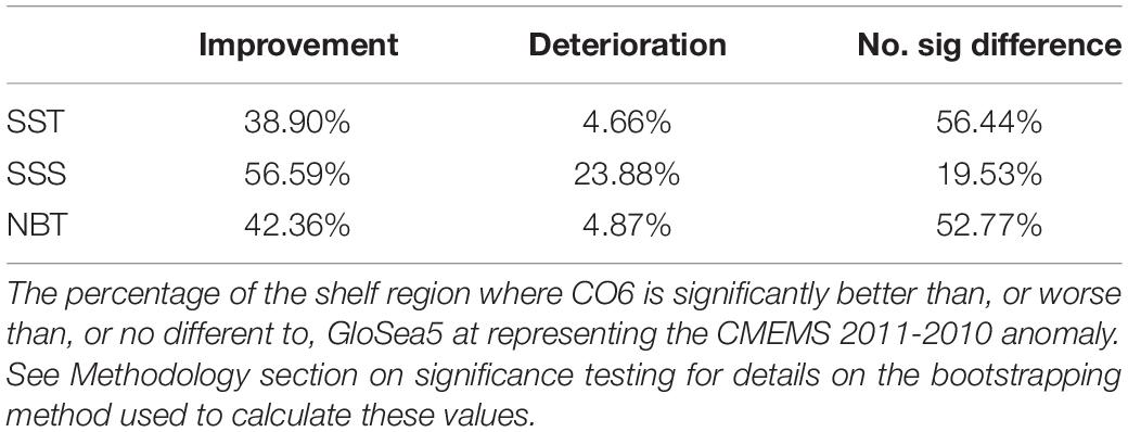
Table 3. Significance of improvements in the 2011-2011 anomaly between CO6 and GloSea5 when compared to CMEMS.
GloSea5 is able to forecast the general spatial patterns of the (2011-2010) SSS difference with a spatial correlation of 0.63 with CMEMS (Figures 10d,e). This reflects both having the greatest salinity anomaly along the southern North Sea, slight negative anomalies in parts of the Celtic and Irish Sea, and weakly positive anomalies over the rest of the shelf. GloSea5 also represents the SSS of the Norwegian Trench relatively well. The GloSea5 shelf mean SSS (2011-2010) anomaly is weaker (0.10, Table 2) than in CMEMS (0.19). There are important details that differ between the GloSea5 and the CMEMS SSS anomalies. The eastern English Channel has a much greater SSS anomaly in GloSea5 than in the CMEMS reanalysis. The region of high SSS anomaly does not extend up the Jutland Peninsula in GloSea5. The region of low or negative SSS anomaly in CMEMS in the Northern Irish Sea, and western northern and central North Sea are absent in GloSea5. This again reflects the differences in circulation.
The CO6 ensemble mean SSS (2011-2010) anomaly is in better agreement with CMEMS (Figures 10d,f). The shelf spatial pattern correlation significantly increases to 0.76 (see Table 4), and the shelf SSS anomaly mean also improves (0.15, Table 2). There is an improvement in the spatial representation of many features of the SSS (2011-2010) anomaly in CO6. There is a good agreement in the Irish and Celtic Seas. There is no significant CO6 salinity difference between the years in the northern Irish Sea, which agrees with the near-zero salinity difference in CMEMS. The eastern English Channel and south western North Sea have a similar patterns and magnitude of SSS anomaly in CMEMS and CO6, which contrasts with GloSea5. The region of high salinity water in the southern and eastern North Sea extends up into the Skagerrak in a similar manner. There is a considerable difference in the SSS anomaly in the Norwegian Trench (adjacent to, but not included in, the shelf region) between CO6 and CMEMS – CO6 is degraded compared to GloSea5. In this region CMEMS has a low, or negative SSS anomaly between the 2 years in the southern Norwegian Trench, CO6 predicts 2011/2012 to be much saltier than 2010/2011 (GloSea5 is closer to CMEMS). This region is strongly influenced by the complex Baltic Sea exchange, which is treated as a climatology in CO6. CO6 agrees well with CMEMS in the regions of low salinity anomalies in the North Sea (or no significant difference between the years), including the Dooley Current, the Norfolk Banks, and offshore of the German Bight, west of Denmark.
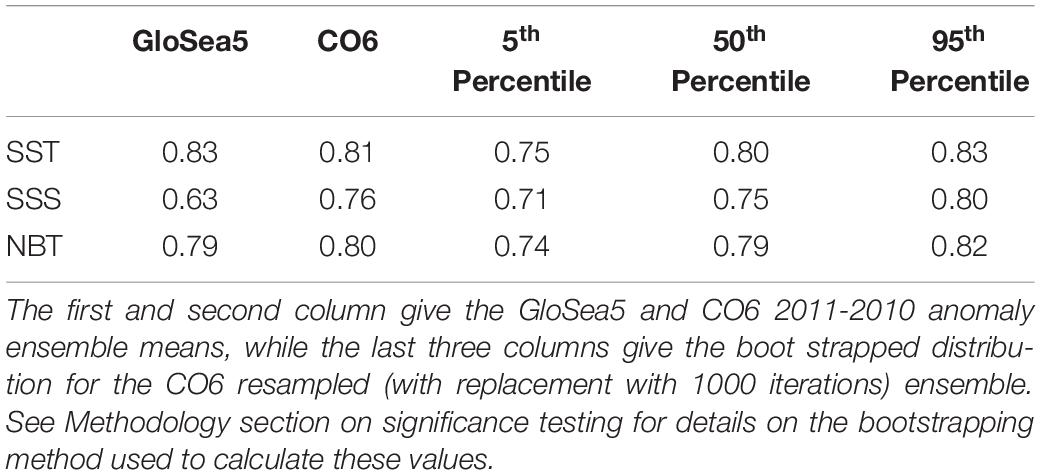
Table 4. The spatial correlation of the GloSea5 and CO6 2011-2011 anomaly with CMEMS 2011-2010 anomaly over the shelf region.
Discussion
We have assessed the GloSea5 simulation of the NWS winter mean climatology, winter evolution and deterministic skill. We have explored the persistence of winter conditions on the NWS, and asked whether GloSea5 deterministic skill improves upon it. We noted that limitations in the GloSea5 representation of the NWS circulation limited its ability to simulate the temperature and salinity fields. We have also explored how improving the representation of the NWS by downscaling may lead to an improved forecast.
We use the CMEMS v4 reanalysis as our “observational” truth. We would prefer to rely solely on independent observations, however most NWS parameters relevant to this study are relatively poorly sampled (compared to SST) which makes variability and predictability difficult to evaluate. The CMEMS reanalysis assimilates satellite SST, and temperature and salinity profiles, and use model physics to spread the observations over a wider area, and has been extensively evaluated (Renshaw et al., 2019). This provides an ideal observations-constrained best-guess estimate of the state of the NWS with which to evaluate. However, errors and biases within CMEMS could affect our model evaluation. This is particularly important for CO6, as both CO6 and CMEMS are based on NEMO CO6, and so it is likely that CO6 and CMEMS share model biases (Abramowitz et al., 2019). If so, the true bias may be under-estimated in CO6, and misinterpreted as an improvement in skill. To reduce the risk of this, we have undertaken additional evaluation against observation products. We have evaluated SST against the OSTIA SST analysis. Both OSTIA and CMEMS assimilate satellite SST, and so they are very similar, and so OSTIA supports the conclusions drawn by the evaluation against CMEMS for both the climatological winter bias (Supplementary Figure 7b) and the difference between 2011 and 2010 (Supplementary Figure 14c). We have evaluated surface salinity against a Copernicus Multivariate Salinity Analysis (CMSA; Droghei et al., 2018). This is product has relatively large analysis errors, which decrease with distance from the coast (∼70% of the NWS has an analysis error >0.5 psu, Supplementary Figure 2), which makes it inappropriate to use to evaluate predictability or the difference between 2 years. However, if these errors are random, they may cancel out when considering a climatological mean. Care must be taking when considering the evaluation against this product, however, it is interesting CMSA also shows the fresh bias seen in the Irish Sea, English Channel and Southern Bight (Supplementary Figure 7e) that is seen when evaluating against CMEMS (Figure 1E). The EN4 data is also relatively sparse for a single winter, is also not very well suited to estimate predictability or the difference between years. However, when evaluating over many years, most of the NWS is filled, allowing an assessment of the climatological bias. As many grid boxes are comparing a single, or few winters, care must be taken when interpreting these results. The GloSea5 salinity bias estimates from EN4 appear to have a similar spatial pattern to those of the CMEMS (Supplementary Figures 7d,f), showing salty biases around Scotland and Ireland, along the European Coast, and in the central North Sea, and fresh biases in the (sparsely sampled) Irish Sea, English Chanel, and offshore of the West Frisian Islands (55°N 4°E). When considering the difference between 2011 and 2010, there are very few observations (Supplementary Figures 14a,b), however, they appear to be in agreement with CMEMS (Supplementary Figures 14c,d) with saltier and warmer values in the German Bight than in the North Sea and a similar east-west temperature and salinity pattern at 59N. Given the limitations of these additional evaluations, we do not include them in the body of the paper (figures are available in the Supplementary Materials and are described in the Appendices) and mainly use them to support our use of the CMEMS reanalysis as our “observed” truth.
We found a general agreement between GloSea5 and CMEMS NWS circulation, but there are several pertinent differences in residual circulation between GloSea5 (based on the global NEMO ORCA025 implementation) and the shelf seas model NEMO CO6 (the shelf seas model used in CMEMS and CO6). We highlighted the differences in residual circulation in the southern North Sea, English Channel and Irish Sea, and the associated tracer distribution (salinity and to a lesser extent, temperature). The incorrect southward transport through the Irish Sea is likely to contribute to its lower salinity as there is less (saline) oceanic water crossing the Celtic Sea into the Irish Sea – this is supported by the GloSea5 patterns in the correlations between salinity and transport (Supplementary Figures 11a,c,e). The GloSea5 Irish Sea to English Channel circulation structure then feeds this fresher water into the English Channel, which, with the differences in the circulation pattern in the southern North Sea, helps explain the differences in the temperature and salinity plume through the Dover Strait, and the temperature and salinity structure in the southern North Sea. The waters in the English Channel and southern North Sea have a different origin in GloSea5 and in reality (and CMEMS, CO6), and this will affect the variability modelled here, which may explain the poorer predictability in this region.
Correlations between the local regional and winter mean salinity, and the transport estimates for GloSea5 (Supplementary Figures 11a,c,e) and CMEMS (Supplementary Figures 11b,d,f) also support these conclusions about the role of circulation. In GloSea5, the Celtic Sea and English Channel are fresher when the southward (i.e., negative) Irish Sea transport is strongest, while the Irish Shelf region is more salty (Supplementary Figure 11a). Conversely, in CMEMS, where the Irish Sea transport is normally northwards (i.e., positive), stronger flow is correlated with fresher water in the Irish and Shetland Shelf regions, and the Northern North Sea (Supplementary Figure 11b). The differences in these correlations patterns (c.f. Supplementary Figures 11a–f) reflect the differences in the transport pathways between GloSea5 and CMEMS. The GloSea5 correlations between the local rivers and SSS are weak in most regions, supporting our assertion that interannual salinity variability is driven by circulation variability rather than rivers. This is also the case in CMEMS which uses climatological rivers, however, it may not be true in reality. The newer version of the CMEMS reanalysis (v5) uses variable rivers.
Tides can help drive the residual circulation (e.g. Robinson, 1983), and so the lack of tides in GloSea5 may help explain the differences in its residual circulation, when compared to CMEMS and CO6. We undertook a preliminary investigation (running CO6 with and without tides) which led to another research study (Tinker et al. 2021, in prep). In that study, we show the effect of the (absences and presence of) tides on the mean circulation and temperature and salinity bias patterns, and explore the underlying tidal mechanisms that drive these differences.
North West European shelf persistence (which is well simulated by GloSea5) is an important component of predictability. The ocean temperatures and salinities adjacent the NWS tend to have high persistence, and the propagation of anomalies can aid NWS persistence (Figure 6). However, differences in the temperature and salinity response to atmosphere (and riverine) conditions lead to differences in the persistence on the NWS. The NWS persistence, as quantified in this paper, may be a sufficient basis for some marine seasonal forecast application.
In the open ocean, the temperature anomalies are spatially large and slow moving, perhaps caused by the large-scale atmosphere conditions and deep mixed layer depths resisting temperature changes. This allows for high oceanic temperature persistence. The propagation of these oceanic temperature anomalies onto the shelf can aid NWS temperature persistence locally. As the shelf is much shallower than the oceanic winter mixed layer depth, the atmosphere can have a greater effect on the temperature of the shelf water. As the oceanic anomalies are advected around the NWS, they become increasingly decorrelated from the open ocean conditions, which reduces persistence. The more remote a location is from the open ocean, the more important local conditions are. For example, the lower persistence of the southern North Sea reflects its very shallow and dynamical nature as much as its remoteness from the North Atlantic.
Salinity is relatively conservative compared to temperature as it has a weaker response to the atmospheric conditions. Advection plays a greater role for ocean salinity anomalies, and so the anomalies are often on the spatial scale of the circulation - this leads to smaller scale anomalies adjacent to the NWS than for temperature. Due to the typical rates of advection, they tend to move slowly, giving high persistence. On the shelf, salinity can be substantially modified by river forcing which tends to reduce the persistence in (and down-stream of) coastal regions. The shelf tends to have important topographically constrained circulation with little variability in current direction and location. This provides pathways for salinity anomalies to be advected in a fairly predictable manner. This can further reduce Eulerian persistence (i.e., the northern North Sea) but can allow high Lagrangian persistence.
Lagrangian SSS persistence is larger than Eulerian persistence in the north-western North Sea (Figure 6). In this region the circulation is fairly strong and invariant (in direction and configuration) and so advecting the November anomalies with a climatological depth mean current field improves the persistence. As the water flows around Ireland and Scotland before flowing into the northern North Sea, the local rivers can cause small scale salinity anomalies which further enhance Lagrangian persistence (relative to Eulerian Persistence). Other regions of more variable flow have little improvement in persistence between the Eulerian and Lagrangian. Regions with lower mean flow, spatially larger salinity anomalies and less river influence tend to have high persistence and little difference between Eulerian and Lagrangian Persistence.
With only 2 years of CO6 to compare, we are unable to assess how downscaling affects the deterministic skill. CO6 has an improved representation of NWS processes (compared to GloSea5), with a more realistic circulation (Figure 8) and advective pathways. This reflects the improved mean temperature and salinity distribution (Supplementary Figures 5, 6). Circulation pathways provide a mechanism for advecting anomalies around the NWS. For example, a fresh anomaly in the Celtic Sea should advect into the Irish Sea and English Channel, however, the incorrect GloSea5 circulation would not allow this. The more realistic downscaled advective pathways may improve predictability for some variables in some regions. The improvements in the circulation in the Irish Sea, English Channel, and southern North Sea suggest salinity, and also, temperature predictability may be improved by downscaling. The magnitude of the northern North Sea circulation is also improved in CO6, which may lead in improved predictability in this region – consistent with the increased SSS persistence when considering CMEMS advection (c.f. SSS Eulerian and Lagrangian Persistence in Figures 6e,f).
In seasonal forecasting it is common to think of the seasonal anomaly, rather than the full field values. In many instances it is possible to treat the two as independent, and thus any biases in the mean climatology do not affect the skill of the system at simulating the anomalies. The residual circulation is an example where the climatology is as important as the anomalies. As GloSea5 has the climatological residual circulation incorrect, the predicted salinity anomalies are systematically incorrect in places, reducing the predictability.
Marine seasonal forecasting is established in Australia (Hobday et al., 2011; Eveson et al., 2015; Brodie et al., 2017) and the United States (Anderson and Beer, 2009; Burke et al., 2013; Kaplan et al., 2016; Mills et al., 2017; Liu et al., 2018), with a mature research community, established operational forecasts and active end-user and stake holder networks. The tidal nature of the NWS has hampered similar development in Europe, and its subdivision into different territorial waters has hampered uptake (Payne et al., 2017). However, the scientific, modelling and technical capabilities are maturing (Tinker et al., 2018), and there is increasing interest in the research community. It is now the time to start to identify potential end-users of a possible European marine seasonal forecasting service and seed a network of such stake holders. User engagement is essential for the development of a useful service, with clear two-way communication of user requirements and scientific capability. We hope that the results of this paper allow such discussions to begin. Question such as “given the predictability and persistence of X at Y, how would you use a seasonal forecast in your sector?” and “What are the parameters/areas/lead times/skill levels are important for your business?” will be vital for the development of such a service. Our quantification of some of these points can provide a basis for such discussions.
We have given an assessment of the GloSea5 NWS winter predictive skill and have shown that its circulation is limiting skill in places. We have also explored how dynamic downscaling improves the circulation - further research is required to assess whether it will improve the predictive skill. If it does, and skilful forecasts of NWS winter temperature and salinity are possible, there are a range of potential users who would benefit. Tinker et al. (2018) suggested three possible approaches to NWS seasonal forecasting – the direct use of the global seasonal forecasting system, using statistical or empirical forecasts to add value to the global seasonal forecasts, or by dynamical downscaling of global seasonal forecasts. These can be thought of as using the forecast directly (with or without downscaling) or using the forecast to drive an empirical or statistical model to provide a forecast. For example, some specific commercial species have a life cycle or food web which is sensitive to near-bottom temperature (see e.g. Pörtner and Farrell, 2008; Dulvy et al., 2008; Pörtner and Peck, 2010; Jones et al., 2015; Pinnegar et al., 2017). Predicting seasonal temperatures may be directly applicable to these species, which would be beneficial to fishers and fisheries managers. Marine spatial planners and, and those responsible for the management of marine protected areas could also benefit from such forecasts. The sea-floor gas distribution network is affected by temperatures, and so seasonal forecasts may allow market planning. One of the longest running high profile marine ecological forecast products uses temperature forecasts directly - the NOAA Coral Reef Heat Stress Outlook (Liu et al., 2017) provides forecasts of coral bleaching events based on temperature forecasts (Payne et al., 2019). While there are no coral reefs on the NWS, this approach may be applied to other heat sensitive species and ecosystems. Using NWS temperature and salinity seasonal forecasts as a basis for other empirical model-based forecasts, would allow a much wider range of potential users. For example, an empirical model of the dynamic habitat of the southern bluefin tuna (Thunnus maccoyii) within the Great Australian Bight has been linked to a seasonal forecast system, with lead times of 3-4 months (Hobday et al., 2011; Eveson et al., 2015). This forecast was one of the earliest marine environmental seasonal forecasts, and has been giving fishery managers and fisher valuable insights into likely tuna distribution ever since.
Conclusion and Further Work
We compared the CMEMS reanalysis climatology with GloSea5 and found:
• GloSea5 simulates the climatological spatial patterns and winter evolution of NWS SST and SSS reasonably well.
• The winter mean circulation is generally well represented, but localised differences lead to important impacts on the overall NWS simulation.
◦ There is a flow reversal in the Irish Sea, and differences in the English Channel and into the southern North Sea.
◦ The GloSea5 winter climatological salinity (and temperature) distribution is affected by these differences, typically with colder and fresher water than in CMEMS in these regions.
◦ The GloSea5 deterministic skill is reduced in the same regions, particularly for SSS, but also for SST in a smaller region (just the southern North Sea).
◦ GloSea5 has a greater northern North Sea inflow, which results in a positive salinity bias (GloSea5 too salty) and a reduced deterministic skill locally. The reduced northern North Sea SST deterministic skill may also be related to the differences in the northern North Sea inflow.
We quantified the NWS winter persistence:
• The NWS exhibits relatively high persistence for temperature and salinity (r > 0.6) over most of the NWS, with regions of lower persistence for temperature in the southern North Sea, and for salinity in important transport pathways. Advection is important for salinity persistence, particularly in the northeast North Sea – we show this with the Lagrangian persistence, which is much greater than Eulerian persistence in the region for salinity.
We assessed GloSea5 prediction skill and compared it to this persistence:
• The GloSea5 SST deterministic skill is slightly higher than persistence over most of the NWS, apart from the North Sea (north of 56 °N). Salinity deterministic skill is much higher than Eulerian persistence along the North Sea northern inflow route (r > 0.3), but not when considering Lagrangian persistence. Salinity deterministic skill is typically lower than persistence in the rest of the NWS.
• The direct use of GloSea5 output is suitable for NWS winter seasonal prediction in some regions for some variables. For example, along the route of the northern North Sea inflow (around western Ireland, Scotland, and into the north western North Sea), SST and SSS have good deterministic skill. Despite the incorrect circulation affecting the climatological SST in the Celtic Sea, western English Channel and Irish Sea, there is also good deterministic skill in these regions, which may be used with care. However, GloSea5 does not show much improvement over (Lagrangian) persistence in many regions. This, in part, reflects the considerable NWS persistence.
We show that GloSea5 is fit for purpose as the basis for a dynamically downscaled winter seasonal prediction.
Finally, we dynamically downscaled the seasonal prediction of two winters:
• Dynamical downscaling improves the climatological NWS circulation compared to GloSea5. Downscaling corrects the southward Irish Sea transport, improves circulation of the English Channel and southern North Sea.
• Correcting these circulation pathways improves the spatial correlation of the mean salinity anomaly pattern (the winter mean salinity difference between the 2 years of the case study). The spatial correlation of the GloSea5 temperature pattern is good (r > 0.8), so there is little statistical improvement when downscaling temperature. However, the downscaled pattern is more physically consistent with the observations than in GloSea5 (e.g., warm water plumes in the Irish Sea, English Channel and into the southern North Sea, not visible in the anomaly plots in Figure 9).
• The deterministic skill cannot be assessed from our case study, but improvements in the circulation provide a mechanism that may allow downscaling to improve the deterministic skill for temperature (particularly in the southern North Sea) and salinity across the NWS.
• We conclude that the improvements to the simulation of the NWS afforded by dynamically downscaling GloSea5 may improve the deterministic skill of NWS winter predictions, including salinity and temperature predictability in the Irish Sea, English Channel, and southern North Sea, and perhaps in the northern North Sea.
We have focussed on the seasonal predictability of winter temperature and salinity on the NWS. Giving a complete assessment of the NWS seasonal predictability is a very large research topic, and beyond the scope of this paper. Future research could focus on other seasons and lead times, the prediction skill of the downscaling from the full 23 years, the predictability of sea level (both the seasonal mean and surge events) and persistence for other season and lead times. Seasonal forecasting is also carried out using multiple ensemble forecast systems (e.g., Hemri et al., 2020) – this could also be assessed with the NWS context. Similar research could also be undertaken with regional surge, wave and biogeochemical modelling systems, as well as considering the decadal timescale (e.g., the Met Office Decadal Climate Prediction System version 4 (DePreSys4); Scaife et al., 2021 in review).
Data Availability Statement
GloSea5
GloSea5 (and the more recent GloSea6) data are available from the Copernicus Climate Change Service (C3S; https://climate.copernicus.eu/, product type: seasonal forecast; dataset: seasonal forecast monthly statistics on single levels; Originating centre: UK Met Office; Year: 2018).
CMEMS data
The CMEMS data are available from the Copernicus Marine Environmental Monitoring Service (CMEMS: https://marine.copernicus.eu) and can be searched using the given product identifier. The datasets are updated periodically, and so the version used in this study may no longer be available.
CMEMS reanalysis: NWSHELF_MULTIYEAR_PHY_004_009.
OSTIA SST analysis: SST_GLO_SST_L4_REP_OBSERVATIO NS_010_011.
CMEMS Multivariate Salinity Analysis: MULTIOBS_GLO_ PHY_S_SURFACE_MYNRT_015_013.
EN4 quality-controlled temperature and salinity profile data
The EN4 dataset is available from the Met Office: https://www.metoffice.gov.uk/hadobs/en4/
CO6
Not available.
Author Contributions
JT undertook the modelling and analysis. LH advised on statistics and seasonal forecasting. Both authors designed the experiment and analysis and wrote the manuscript.
Funding
Both authors were supported by the Met Office Hadley Centre Climate Programme funded by the BEIS and Defra.
Conflict of Interest
The authors declare that the research was conducted in the absence of any commercial or financial relationships that could be construed as a potential conflict of interest.
Publisher’s Note
All claims expressed in this article are solely those of the authors and do not necessarily represent those of their affiliated organizations, or those of the publisher, the editors and the reviewers. Any product that may be evaluated in this article, or claim that may be made by its manufacturer, is not guaranteed or endorsed by the publisher.
Acknowledgments
We would like to thank several people who advised and offered scientific insights that helped shape this study. Useful discussion with Adam Scaife helped in the early stages of this study, and with the final version of the manuscript. Nicky Stringer provided GloSea5 NAO values and code, and Rosie Eade advised on the Ratio of Predictable Components. Enda O’Dea provided technical advice on NEMO CO6. Claire O’Neill ran a NEMO surge simulation of the NWS with and without tides that helped show the impact of tides on the mean NWS circulation - this led to another paper of which she is a co-author. Matt Palmer and Richard Wood provided helpful comments on the manuscript. Stephen Dye, Rosa Barciela, Richard Wood, and Mark Payne have all helped provide context and insights into the user requirement for such a study. And finally, we would like to thank the reviewers who gave such useful and constructive criticism, which has led to a stronger paper.
Supplementary Material
The Supplementary Material for this article can be found online at: https://www.frontiersin.org/articles/10.3389/fmars.2021.698997/full#supplementary-material
Footnotes
- ^ CMEMS product code: NORTHWESTSHELF_REANALYSIS_PHY_PHY_004 _009
- ^ CMEMS product code: CMEMS-BALTICSEA-ANALYSIS_FORECAST_PHYS_003_008
- ^ http://marine.copernicus.eu/services-portfolio/access-to-products/
References
Abramowitz, G., Herger, N., Gutmann, E., Hammerling, D., Knutti, R., Leduc, M., et al. (2019). ESD Reviews: model dependence in multi-model climate ensembles: weighting, sub-selection and out-of-sample testing. Earth Syst. Dyn. 10, 91–105. doi: 10.5194/esd-10-91-2019
Anderson, J. J., and Beer, N. W. (2009). Oceanic, riverine, and genetic influences on spring chinook salmon migration timing. Ecol. Appl. 19, 1989–2003. doi: 10.1890/08-0477.1
Arribas, A., Glover, M., Maidens, A., Peterson, K., Gordon, M., MacLachlan, C., et al. (2011). The GloSea4 ensemble prediction system for seasonal forecasting. Monthly Weather Rev. 139, 1891–1910. doi: 10.1175/2010MWR3615.1
Axell, L., Golbeck, I., Jandt, S., and Izotova, J. (2017). Baltic Sea Production Centre Balticsea_Reanalysis_Phys_003_008. Available online at: https://resources.marine.copernicus.eu/documents/QUID/CMEMS-BAL-QUID-003-008.pdf (accessed July 15, 2021).
Berndtsson, R., Jinno, K., Kawamura, A., Larson, M., and Niemczynowicz, J. (1994). Some Eulerian and Lagrangian statistical properties of rainfall at small space-time scales. J. Hydrol. 153, 339–355. doi: 10.1016/0022-1694(94)90198-8
Best, M. J., Pryor, M., Clark, D. B., Rooney, G. G., Essery, R. L. H., Ménard, C. B., et al. (2011). The joint UK land environment simulator (JULES), model description – Part 1: energy and water fluxes. Geosci. Model Dev. 4, 677–699. doi: 10.5194/gmd-4-677-2011
Brodie, S., Hobday, A. J., Smith, J. A., Spillman, C. M., Hartog, J. R., Everett, J. D., et al. (2017). Seasonal forecasting of dolphinfish distribution in eastern Australia to aid recreational fishers and managers. Deep Sea Res. Part II. Top. Stud. Oceanogr. 140, 222–229. doi: 10.1016/j.dsr2.2017.03.004
Brown, A., Milton, S. F., Cullen, M., Golding, B., Mitchell, J., and Shelly, A. (2012). Unified modeling and prediction of weather and climate: a 25-year journey. Bull. Am. Meteorol. Soc. 93, 1865–1877. doi: 10.1175/BAMS-D-12-00018.1
Burke, B. J., Peterson, W. T., Beckman, B. R., Morgan, C., Daly, E. A., and Litz, M. (2013). Multivariate models of adult pacific salmon returns. PLoS One 8:e54134. doi: 10.1371/journal.pone.0054134
Clark, R. T., Bett, P. E., Thornton, H. E., and Scaife, A. A. (2017). Skilful seasonal predictions for the European energy industry. Environ. Res. Lett. 12:024002. doi: 10.1088/1748-9326/aa57ab
Dagestad, K. F., Röhrs, J., Breivik, O., and Ådlandsvik, B. (2018). OpenDrift v1.0: a generic framework for trajectory modelling. Geosci. Model Dev. 11, 1405–1420. doi: 10.5194/gmd-11-1405-2018
Dee, D. P., Uppala, S. M., Simmons, A. J., Berrisford, P., Poli, P., Kobayashi, S., et al. (2011). The ERA-Interim reanalysis: configuration and performance of the data assimilation system. Q. J. R. Meteorol. Soc. 137, 553–597. doi: 10.1002/qj.828
Droghei, R., Buongiorno Nardelli, B., and Santoleri, R. (2018). A new global sea surface salinity and density dataset from multivariate observations (1993–2016). Front. Mar. Sci. 5:84. doi: 10.3389/fmars.2018.00084
Dulvy, N. K., Rogers, S. I., Jennings, S., Stelzenmüller, V., Dye, S. R., and Skjoldal, H. R. (2008). Climate change and deepening of the North Sea fish assemblage: a biotic indicator of warming seas. J. Appl. Ecol. 45, 1029–1039. doi: 10.1111/j.1365-2664.2008.01488.x
Eveson, P. E., Hobday, A. J., Hartog, J. R., Spillman, C. M., and Rough, K. M. (2015). Seasonal forecasting of tuna habitat in the Great Australian Bight. Fish. Res. 170, 39–49. doi: 10.1016/j.fishres.2015.05.008
Good, S. A., Martin, M., and Rayner, N. A. (2013). EN4: quality controlled ocean temperature and salinity profiles and monthly objective analyses with uncertainty estimates. J. Geophys. Res. Oceans 118, 6704–6716. doi: 10.1002/2013JC009067
Hemri, S., Bhend, J., Liniger, M. A., Manzanas, R., Siegert, S., Stephenson, D. B., et al. (2020). How to create an operational multi-model of seasonal forecasts? Clim. Dyn. 55, 1141–1157. doi: 10.1007/s00382-020-05314-2
Hermans, T. H. J., Tinker, J., Palmer, M. D., Katsman, C. A., Vermeersen, B. L. A., and Slangen, A. B. A. (2020). Improving sea-level projections on the Northwestern European shelf using dynamical downscaling. Clim. Dyn. 54, 1987–2011. doi: 10.1007/s00382-019-05104-5
Hjort, J. (1914). Fluctuations in the Great Fisheries of Northern Europe Viewed in Light of Biological Research. Rapports et Procés Verbaux Des Réunions de Conseil International Pour l’Exploration de La Mer, Vol. 20. Copenhague: Hoest & Fils, 1–228.
Hobday, A. J., Hartog, J. R., Spillman, C. M., and Alves, O. (2011). Seasonal forecasting of tuna habitat for dynamic spatial management. Can. J. Fish. Aquatic Sci. 68, 898–911. doi: 10.1139/f2011-031
Hobday, A. J., Spillman, C. M., Paige Eveson, J., and Hartog, J. R. (2016). Seasonal forecasting for decision support in marine fisheries and aquaculture. Fish. Oceanogr. 25, 45–56. doi: 10.1111/fog.12083
Hunke, E. C., and Lipscomb, W. H. (2010). CICE: The Sea Ice Model Documentation and Software User’s Manual, Version 4.1. Technical report LA-CC-06-012. Los Alamos, NM: Los Alamos National Laboratory.
Hurrell, J. W. (1995). Decadal trends in the North Atlantic Oscillation – regional temperatures and precipitation. Science 269, 676–679. doi: 10.1126/science.269.5224.676
Jones, M. C., Dye, S. R., Pinnegar, J. K., Warren, R., and Cheung, W. W. L. (2015). Using scenarios to project the changing profitability of fisheries under climate change. Fish Fish. 16, 603–622. doi: 10.1111/faf.12081
Kaplan, I. C., Williams, G. D., Bond, N. A., Hermann, A. J., and Siedlecki, S. A. (2016). Cloudy with a chance of sardines: Forecasting sardine distributions using regional climate models. Fish. Oceanogr. 25, 15–27. doi: 10.1111/fog.12131
King, N. G., Wilmes, S. B., Smyth, D., Tinker, J., Robins, P. E., Thorpe, J., et al. (2021). Climate change accelerates range expansion of the invasive non-native species, the Pacific oyster, Crassostrea gigas. ICES J. Mar. Sci. 78, 70–81. doi: 10.1093/icesjms/fsaa189
Large, W., and Yeager, S. (2009). The global climatology of an interannually varying air–sea flux data set. Clim. Dyn. 33, 341–364. doi: 10.1007/s00382-008-0441-3
Liu, G., Mark Eakin, C., Chen, M., Kumar, A., De La Cour, J. L., Heron, S. F., et al. (2018). Predicting heat stress to inform reef management: NOAA coral reef watch’s 4-month coral bleaching outlook. Front. Mar. Sci. 5:57. doi: 10.3389/fmars.2018.00057
Liu, G., Skirving, W. J., Geiger, E. F., De La Cour, J. L., Marsh, B. L., Heron, S. F., et al. (2017). NOAA Coral Reef Watch’s 5km Satellite Coral Bleaching Heat Stress Monitoring Product Suite Version 3 and Four-Month Outlook Version 4. Cairns City, QLD: Reef Encounter.
MacLachlan, C., Arribas, A., Peterson, K. A., Maidens, A., Fereday, D., Scaife, A. A., et al. (2014). Global Seasonal forecast system version 5 (GloSea5): a high-resolution seasonal forecast system. Q. J. R. Meteorol. Soc. 141, 1072–1084. doi: 10.1002/qj.2396
Maidens, A., Arribas, A., Scaife, A. A., Maclachlan, C., Peterson, D., and Knight, J. (2013). The influence of surface forcings on prediction of the north atlantic oscillation regime of winter 2010/11. Monthly Weather Rev. 141, 3801–3813. doi: 10.1175/MWR-D-13-00033.1
Megann, A., Storkey, D., Aksenov, Y., Alderson, S., Calvert, D., Graham, T., et al. (2014). GO5.0: the joint NERC–Met Office NEMO global ocean model for use in coupled and forced applications. Geosci. Model Dev. 7, 1069–1092. doi: 10.5194/gmd-7-1069-2014
Mills, K. E., Pershing, A. J., and Hernández, C. M. (2017). Forecasting the seasonal timing of Maine’s lobster fishery. Front. Mar. Sci. 4:337. doi: 10.3389/fmars.2017.00337
Nagy, H., Pereiro, D., Yamanaka, T., Cusack, C., Nolan, G., Tinker, J., et al. (2021). The Irish Atlantic CoCliME case study configuration, validation and application of a downscaled ROMS ocean climate model off SW Ireland. Harmful Algae (in press). doi: 10.1016/j.hal.2021.102053
O’Dea, E., Furner, R., Wakelin, S., Siddorn, J., While, J., Sykes, P., et al. (2017). The CO5 configuration of the 7 km Atlantic Margin Model: large-scale biases and sensitivity to forcing, physics options and vertical resolution. Geosci. Model Dev. 10, 2947–2969. doi: 10.5194/gmd-10-2947-2017
Oki, T., Nishimura, T., and Dirmeyer, P. (1999). Assessment of annual runoff from land surface models using total runoff integrating pathways (TRIP). J. Meteorol. Soc. Jpn. 77, 235–255. doi: 10.2151/jmsj1965.77.1b_235
Oki, T., and Sud, U. C. (1998). Design of total runoff integrating pathways (TRIP) – a global river channel network. Earth Interact. 2, 1–36. doi: 10.1175/1087-3562(1998)002<0001:dotrip>2.0.co;2
Palin, E. J., Scaife, A. A., Wallace, E., Pope, E. C. D., Arribas, A., and Brookshaw, A. (2016). Skillful seasonal forecasts of winter disruption to the U.K. transport system. J. Appl. Meteorol. Climatol. 55, 325–344. doi: 10.1175/JAMC-D-15-0102.1
Payne, M. R., Hobday, A. J., MacKenzie, B. R., and Tommasi, D. (2019). Editorial: seasonal-to-decadal prediction of marine ecosystems: opportunities, approaches, and applications. Front. Mar. Sci. 6:100. doi: 10.3389/fmars.2019.00100
Payne, M. R., Hobday, A. J., MacKenzie, B. R., Tommasi, D., Dempsey, D. P., Fässler, S. M. M., et al. (2017). Lessons from the first generation of marine ecological forecast products. Front. Mar. Sci. 4:15. doi: 10.3389/fmars.2017.00289
Pinnegar, J. K., Garrett, A., Simpson, S. D., Engelhard, G. H., and Van der Kooij, J. (2017). Fisheries. MCCIP Sci. Rev. 2017, 73–99. doi: 10.14465/2017.arc10.007-fis
Pörtner, H. O., and Farrell, A. P. (2008). Physiology and climate change. Science 322, 690–692. doi: 10.1126/science.1163156
Pörtner, H. O., and Peck, M. A. (2010). Climate change effects on fishes and fisheries: towards a cause-and-effect understanding. J. Fish Biol. 77, 1745–1779. doi: 10.1111/j.1095-8649.2010.02783.x
Renshaw, R., Wakelin, S. L., Mahdon, R., O’Dea, E., and Tinker, J. (2019). Copernicus Marine Environment Monitoring Service Quality Information Document North West European Shelf Production Centre NORTHWESTSHELF_REANALYSIS_PHYS_004_009. Exeter. Available online at: http://marine.copernicus.eu/documents/QUID/CMEMS-NWS-QUID-004-009.pdf (accessed July 15, 2021).
Roberts-Jones, J., Fiedler, E., and Martin, M. J. (2012). Daily, global, high-resolution SST and sea ice reanalysis for 1985–2007 using the OSTIA system. J. Clim. 25, 6215–6232. doi: 10.1175/JCLI-D-11-00648.1
Robinson, I. S. (1983). Tidally induced residual flows. Elsevier Oceanogr. Ser. 35, 321–356. doi: 10.1016/S0422-9894(08)70505-1
Scaife, A., Hermanson, L., van Niekerk, A., Baldwin, M. P., Belcher, S., Bett, P., et al. (2021). Long range predictability of the length of day and extratropical climate. Nat. Geosci. doi: 10.5194/egusphere-egu21-191
Scaife, A. A., Arribas, A., Blockley, E., Brookshaw, A., Clark, R. T., Dunstone, N., et al. (2014). Skillful long-range prediction of European and North American winters. Geophys. Res. Lett. 41, 2514–2519. doi: 10.1002/2014GL059637
Scaife, A. A., Comer, R. E., Dunstone, N. J., Knight, J. R., Smith, D. M., MacLachlan, C., et al. (2017). Tropical rainfall, Rossby waves and regional winter climate predictions. Q. J. R. Meteorol. Soc. 143, 1–11. doi: 10.1002/qj.2910
Siddorn, J. R. R., and Furner, R. (2013). An analytical stretching function that combines the best attributes of geopotential and terrain-following vertical coordinates. Ocean Modelling 66, 1–13. doi: 10.1016/j.ocemod.2013.02.001
Svensson, C., Brookshaw, A., Scaife, A. A., Bell, V. A., Mackay, J. D., Jackson, C. R., et al. (2015). Long-range forecasts of UK winter hydrology. Environ. Res. Lett. 10:064006. doi: 10.1088/1748-9326/10/6/064006
Taws, S. L., Marsh, R., Wells, N. C., and Hirschi, J. (2011). Re-emerging ocean temperature anomalies in late-2010 associated with a repeat negative NAO. Geophys. Res. Lett. 38:L20601. doi: 10.1029/2011GL048978
Taylor, K. E. (2001). Summarizing multiple aspects of model performance in a single diagram. J. Geophys. Res. 106, 7183–7192. doi: 10.1029/2000jd900719
Tinker, J., Krijnen, J., Wood, R., Barciela, R., and Dye, S. R. (2018). What are the prospects for seasonal prediction of the marine environment of the North-west European Shelf? Ocean Sci. 14, 887–909. doi: 10.5194/os-14-887-2018
Tinker, J., Lowe, J., Pardaens, A., Holt, J., and Barciela, R. (2016). Uncertainty in climate projections for the 21st century northwest European shelf seas. Prog. Oceanogr. 148, 56–73. doi: 10.1016/j.pocean.2016.09.003
Tinker, J., Palmer, M. D., Copsey, D., Howard, T. P., Lowe, J., and Hermans, T. H. J. (2020). Dynamical downscaling of unforced interannual sea-level variability in the North-West European shelf seas. Clim. Dyn. 55, 2207–2236. doi: 10.1007/s00382-020-05378-0
Tonani, M., Pequignet, C., King, R., Sykes, P., McConnell, N., and Siddorn, J. R. (2019). Copernicus Marine Environment Monitoring Service Quality Information Document North West European Shelf Production Centre NORTHWESTSHELF_ANALYSIS_FORECAST_PHYS_004_013. Exeter. Available online at: http://resources.marine.copernicus.eu/documents/QUID/CMEMS-NWS-QUID-004-013.pdf (accessed July 15, 2021).
Vörösmarty, C. J., Green, P., Salisbury, J., and Lammers, R. B. (2000). Global water resources: Vulnerability from climate change and population growth. Science 289, 284–288. doi: 10.1126/science.289.5477.284
Walters, D., Best, M., Bushell, A., Copsey, D., Edwards, J., Falloon, P. D., et al. (2011). The met office unified model global atmosphere 3.0/3.1 and JULES Global Land 3.0/3.1 configurations. Geosci. Model Dev. 4, 919–941. doi: 10.5194/gmd-4-919-2011
Walters, D., Boutle, I., Brooks, M., Melvin, T., Stratton, R., Vosper, S., et al. (2017). The met office unified model global atmosphere 6.0/6.1 and JULES Global Land 6.0/6.1 configurations. Geosci. Model Dev. 10, 1487–1520. doi: 10.5194/gmd-10-1487-2017
Williams, K. D., Harris, C. M., Bodas-Salcedo, A., Camp, J., Comer, R. E., Copsey, D., et al. (2015). The met office global coupled model 2.0 (GC2) configuration. Geosci. Model Dev. 8, 1509–1524. doi: 10.5194/gmd-8-1509-2015
Young, E. F., and Holt, J. T. (2007). Prediction and analysis of long-term variability of temperature and salinity in the Irish Sea. J. Geophys. Res. Oceans 112, 1–18.
Appendices
Estimates of Volume Transport Through Cross-Sections
When considering the NWS circulation, we consider the spatial configuration with depth mean current maps (e.g., Figure 2). However, this does not show the temporal characteristics of the flow, and makes it difficult to quantify the net transport. An alternative solution is to calculate a quantitative time-series of the transport through a cross-section. As our models are Boussinesq, we consider volume transport rather than mass transport. The volume transport can be calculated as the product of the tangential velocity (U) and grid box cross-sectional area (A), and summing up over the grid box of the cross-section:
Given the velocity and area have a temporal mean and varying component:
The time mean transport is not only the product of the mean area and velocity, as there is also a cross term.
This cross term is particularly important in tidal simulations, where both the area (depth of water) and velocity vary substantially from the mean. Therefore, this should be calculated at run time (every time step), or with hourly values. In non-tidal runs (i.e., GloSea5), the cross term is likely to be much smaller, and may be negligible.
We make estimates of the volume transport into the Northern North Sea (between John O’Groats and the Orkneys, and between the Orkneys and the Shetlands), through the Irish Sea and through the English Channel (Supplementary Figure 1). The methodology is different between the CMEMS and GloSea5, and so we consider this as semi-quantitative. CMEMS calculates the instantaneous volume transport through a number of cross-sections at run time. These are saved as 25 h means (to approximately remove the tidal signal). We have averaged this 25-h means into winter mean transport through the available cross-sections, noting that monthly means based on 25-h means introduces an error.
GloSea5 does not calculate the volume transport, and we only have monthly mean ocean fields. As GloSea5 does not include tides, we make transport estimates by assuming the cross-term is negligible. For simplicity, we choose cross-sections that follow the GloSea5 ocean (ORCA025) grid, while this has little impact on the Irish Sea and English Channel Cross section, the northern North Sea cross section is different. This cross section now is between Peterhead and the Shetlands (Supplementary Figure 1). However, given the net rate of volume transport through this cross-section compared to the possible river input between John O’Groats and Peterhead, and the precipitation minus evaporation between John O’Groats, Peterhead and the Shetland, we consider this reasonable and a comparable estimate of the northern North Sea inflow.
When considering NWS salinity variability, we correlate the salinity (regional mean, DJF from the 23 year) with transport across these cross-sections for both the GloSea5 ensemble mean, and CMEMS (Supplementary Figure 11). The difference in these correlation patterns reflects the differences in NWS circulation between GloSea5 and CMEMS, and role of the circulation pathways in the local salinity variability. We also correlated the local regional mean SSS against river input for GloSea5 (CMEMS has climatological rivers, and so have no interannual variability) so show the relative importance of river variability compared to circulation variability for salinity.
Additional Observational Data Sets
We have undertaken additional evaluation against observation datasets to supplement our evaluation against CMEMS. We evaluate SST against the OSTIA SST analysis product, SSS against the CMSA salinity product, and SST and SSS against the EN4 temperature and salinity profile data set.
The OSTIA (Operational Sea-Surface Temperature and Sea-Ice Analysis) SST analysis product (Roberts-Jones et al., 2012) is a predominantly satellite based dataset available via the Copernicus Marine Environmental Monitoring Service (SST_GLO_SST_L4_REP_OBSERVATIONS_010_011). This analysis combines in situ observations with different bias corrected satellite products to reduce the bias of the overall product. We use monthly mean fields between 1994 and 2016.
The Copernicus Multivariate Salinity Analysis (CMSA) consists of global gap-free analyses of the Sea Surface Salinity (SSS) and Sea Surface Density (SSD). It uses a multivariate optimal interpolation algorithm to combines Soil Moisture Ocean Salinity (SMOS) satellite images and in situ salinity measurements with satellite SST information (Droghei et al., 2018). It was developed by the COnsiglio Nazionale delle Ricerche (CNR) and is available through the Copernicus Marine Environmental Monitoring Service (MULTIOBS_GLO_PHY_S_SURFACE_MYNRT_015_013).
The EN4 quality-controlled in situ temperature and salinity profile dataset (Good et al., 2013) (between 1960 and 2020) provides a gridded and non-gridded dataset. There is good global coverage (mainly due to ARGO buoys), however the observations are much sparser on the NWS. Given this sparseness, and the complex bathymetry, coastline, and tidal circulation, we do not use the gridded product. Instead, we assign each observed profile (within the NWS model domain) to the nearest model grid box. When there is more than one profile for a given month and grid box, we average them. We then subtract this from the equivalent model field, to give a sparse field of monthly model minus EN4 biases. These are then averaged into a winter biases (where, for a given year, a winter bias may be made up of 1, 2, or 3 months), and then averaged into a climatological winter bias (where each grid box winter bias may be made of between 1 and 23 winters). Given most grid boxes do not have many years of data, the EN4 dataset is not appropriate for assessing model skill (by performing correlations), also, there are very few grid boxes that sample both 2010/2011 and 2011/2012 winters (as shown in Supplementary Figure 14).
Both CMEMS and OSTIA assimilate satellite SST observations and so are similar to one another, as is their evaluation. The in situ and satellite salinity analysis (CMSA) has errors of ∼1 psu at the coast (Supplementary Figure 2), reducing to ∼0.25 psu with distance from the coast (with ∼95% of the NWS having CMSA errors greater than 0.25 psu and, 50% of the NWS greater the ∼0.6 psu). These uncertainty ranges make it difficult to use the data for model evaluation, and make significance testing pointless. However, assuming the errors are independent and random (not systematic) within these error bars, they may cancel out when averaged over multiple years, and so we cautiously evaluate the GloSea5 minus CMSA mean bias over the 23-year period. The EN4 profile data set is relatively sparse on the NWS, and very few points are sampled repeatedly. Climatologies can be computed from EN4 data over a large proportion of the NWS and these can be used to assess climatological biases. However, there are generally too few grid boxes that are resampled enough to allow predictability (correlations) to be assessed, or the difference between years (as shown in Supplementary Figure 14).
Keywords: North West European Shelf Seas, seasonal predictability, GloSea5, dynamical downscaling, persistence, NEMO Coastal Ocean
Citation: Tinker J and Hermanson L (2021) Towards Winter Seasonal Predictability of the North West European Shelf Seas. Front. Mar. Sci. 8:698997. doi: 10.3389/fmars.2021.698997
Received: 22 April 2021; Accepted: 29 June 2021;
Published: 12 August 2021.
Edited by:
Matthias Gröger, Leibniz Institute for Baltic Sea Research (LG), GermanyReviewed by:
Hagen Radtke, Leibniz Institute for Baltic Sea Research (LG), GermanyChristian Dieterich, Swedish Meteorological and Hydrological Institute, Sweden
Copyright © 2021 Tinker and Hermanson. This is an open-access article distributed under the terms of the Creative Commons Attribution License (CC BY). The use, distribution or reproduction in other forums is permitted, provided the original author(s) and the copyright owner(s) are credited and that the original publication in this journal is cited, in accordance with accepted academic practice. No use, distribution or reproduction is permitted which does not comply with these terms.
*Correspondence: Jonathan Tinker, am9uYXRoYW4udGlua2VyQG1ldG9mZmljZS5nb3YudWs=