Practical Method to Screen Contaminated Holograms of Flocs Using Light Intensity

Submergible digital holographic camera can measure the in situ size and shape of suspended particles, such as complex flocs and biological organisms, without disturbance. As the number of particles in the water column increases, overlapping concentric rings (interference patterns) can contaminate the holographic images. Using light intensity (LI), this study proposes a practical method to assess the degree of contamination and screen out contaminated images. The outcomes from image processing support that LI normalized on a gray scale of 0 (black) to 255 (white) can be a reliable criterion for defining the contamination boundary. Results found that as LI increased, the shape of the particle size distribution shifted from a positively skewed to a normal distribution. When LI was lower than approximately 80, owing to the distortion of particle properties, the settling velocities derived from the contaminated holograms with mosaic patterns were underestimated compared to those from the uncontaminated holograms. The proposed method can contribute to a more accurate estimation of the transport and behavior of cohesive sediments in shallow estuarine environments.

Introduction

Digital holography is an imaging method that records holograms using a charge-coupled device (CCD) camera. The reconstruction of such images is numerically performed using digitized interferograms (Mills and Yamaguchi, 2005). Since the introduction of holography into the scientific community in the 1940s (Gabor, 1948), it has become an indispensable technique used in various fields of fluid mechanics, metrology, and medical imaging (Nayak et al., 2021). Because holography is a proven method that enables the provision of a solution to the limitations of the focal plane, the marine science community has recently adopted it to collect information on the three-dimensional properties of particulate matter (e.g., sediment and plankton) suspended in a water column (e.g., Graham and Nimmo-Smith, 2010; Choi et al., 2018; Nayak et al., 2019; Giering et al., 2020).

The application of holographic techniques to cohesive sediments distributed in coastal environments has been somewhat limited. It is because the high concentration of fine-grained suspended particles greatly reduces the optical transmittance within the water column (Sun et al., 2002). For instance, flocculated cohesive sediments are readily settled and deposited on the bed during slack tides, and then resuspended into the overlying layer during tidal acceleration periods. Such cyclic behaviors form a high-concentration (greater than hundreds of mg l^–1) near-bed layer, which makes it hard to meet the optical transmittance required to acquire the proper hologram and conduct post-processing for image analysis. To overcome this technical problem, several studies have developed a post-processing procedure for background correction and modified segmentation sequences, and suggested the maximum theoretical suspended sediment concentration (SSC) for measurable operation (e.g., Sequoia, 2014; Giering et al., 2020). However, the threshold for capturing proper hologram varies with the local bed properties because the SSC greatly depends on the size and shape of particles (Davies-Colley et al., 2014; Merten et al., 2014), causing difficulties in the accurate detection of complex cohesive sediments.

Owing to the aforementioned technical issues, there is a need to define a widely applicable criterion to assess the degree of contamination and then screen out the contaminated images. Therefore, the main objectives of this study were to: (1) identify a criterion to screen contaminated holograms and (2) evaluate the associated practical method in the view of behaviors (e.g., settling) of flocs in cohesive sediment dynamics.

Materials and Methods

Study Sites and Data Collection

Two study sites representing a tide-dominated estuarine system were selected on the west coast of Korea (Figure 1A): Ganghwa Tidal Flat (GTF) and Geum River Estuary (GRE). In both sites, the bed sediments predominantly consist of fine-grained sediments (clay and silt) supplied from the river. Under a hypertidal regime with a tidal range of up to 10.2 m, the suspended sediments in the water column are repetitively resuspended and settled by tidal currents. Such a dynamic condition is optimal for investigating in situ holograms of fine-grained particles.

FIGURE 1

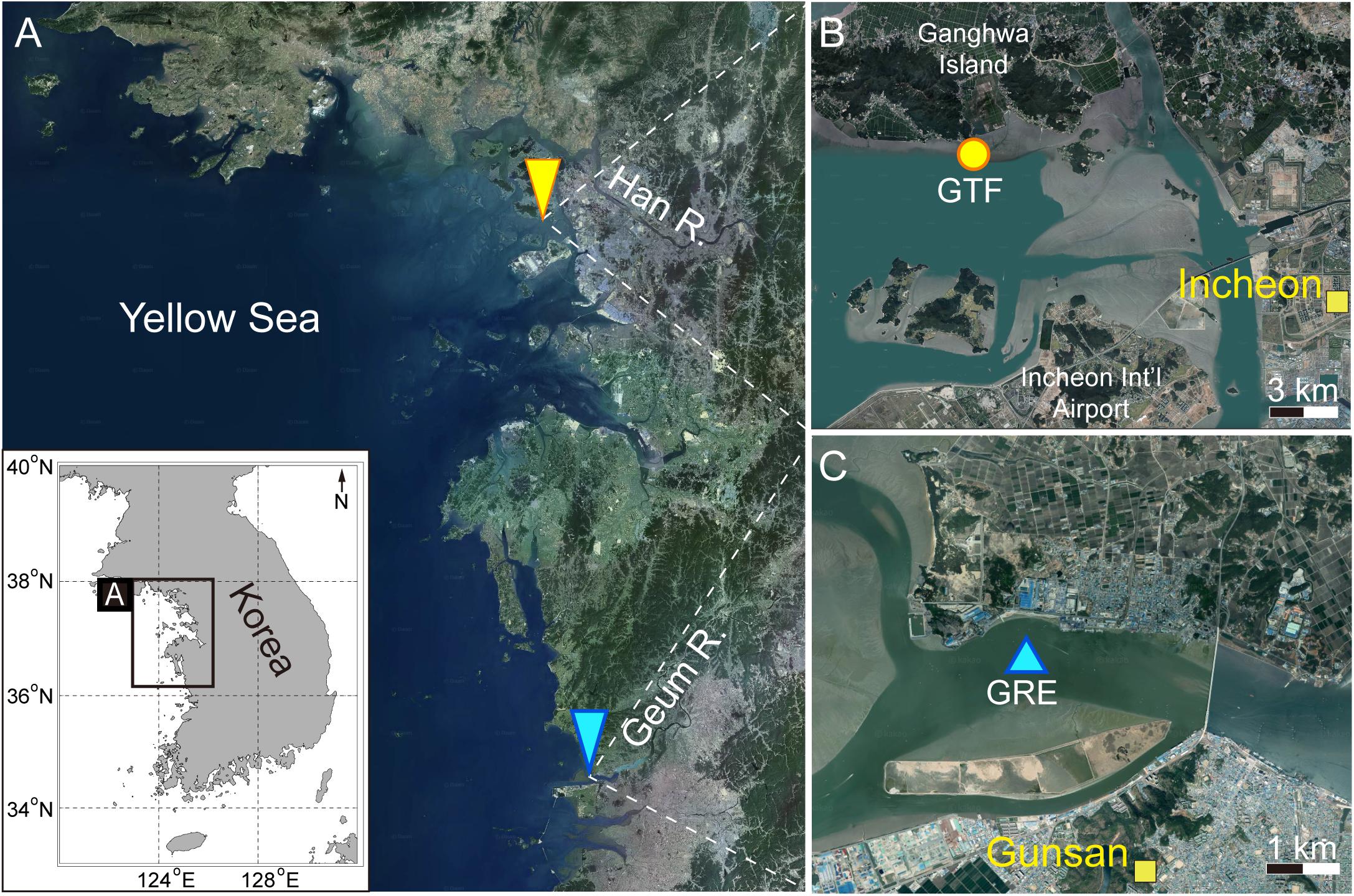
Figure 1. (A) Satellite image showing the study area in Korean Peninsula: (B) Ganghwa tidal flat (GTF) and (C) Geum river estuary (GRE). Sampling stations are marked by the yellow circle in panel (B) and the cyan triangle in panel (C). All satellite images were downloaded from https://map.kakao.com/.

The GTF lies in the estuary of the Han River (Figure 1B). The total surface area of the tidal flats is 302.4 km², and its southern part contains 86% of them extending up to 6 km from the coastline (Woo and Je, 2002). Within the GTF, the mixed (sand and mud) flat is widely distributed, and median particle size (d₅₀) was approximately 17.5 μm, which was measured by a particle-sizing instrument (Malvern, Mastersizer 2000S) in a dispersed state (Table 1). The imaging data were obtained using a submergible digital holographic camera (LISST-Holo, Sequoia Inc.). By installing a path reduction module, the optical path length was reduced from 50 to 10 mm to extend the upper limit of the measurable SSC. The LISST-Holo attached to a H-frame system was deployed at 0.15 m above the bed in the upper tidal flat during October 12–20, 2019. For the analysis, two typical tidal cycles (October 12 and 16) were chosen based on the SSC varying from 53 to 221 mg l^–1.

TABLE 1

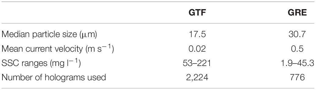
Table 1. Summary on hydrodynamics and sediment properties for Ganghwa Tidal Flat (GTF) and Geum River Estuary (GRE).

The GRE is a 396-km-long drowned river valley with the watershed area of 9,836 km² (Figure 1C; Kim et al., 2006; Figueroa et al., 2019). In the GRE, the sediment was sandy-silt and d₅₀ was 14–58 μm (Ministry of Oceans and Fisheries, 2019). The mean current velocity reached approximately 0.5 m s^–1 during the spring tide (Figueroa et al., 2020). The optical backscattering sensor and LISST-Holo were profiled at intervals of 30 min for 12 h on September 2, 2016, to collect the particle information. With cyclic tidal phases, the SSC in the water column varied in the range of 2–45.3 mg l^–1.

The laboratory water tank experiments have been conducted to convince the in situ results. We used a suspension of known particle size and shape with varying concentration. Details on laboratory experiments are given in Supplementary Figures 1–3.

LISST-Holo

The LISST-Holo is a device designed to measure the properties (e.g., size, number, shape, and volume concentration) of suspended particles (Sequoia, 2014). This device is capable of capturing in situ size (20–2,000 μm) and shape for suspended particles such as complex aggregates and biological organisms (Graham and Nimmo-Smith, 2010; Graham et al., 2012). To visualize the holograms generated from LISST-Holo, several parameters such as exposure, shutter, brightness, gain, and laser power should be balanced. In this study, each parameter was set as the default value suggested by Sequoia Inc. A detailed description of the settings is provided next. The exposure and shutter indicate the amount of light per unit area reaching the surface of the electronic image sensor and of the passed light for a determined period, respectively. Thus, the observed holograms could be contaminated depending on the exposure values modulated by the shutter speed and lens aperture (Sequoia, 2014). In a condition where the suspended particles are freely transported in the water column, the longer the shutter time, the blurrier the hologram. This is because a few microseconds are required to capture the hologram image. If suspended particles move more than half a pixel during that time, the captured image includes the trajectories of the particles, resulting in a blurry hologram. Sequoia (2014) recommended that the current velocity should be lower than 0.5 m s^–1 with a camera shutter of 30 ms and a pixel of 4.4 μm. The brightness is an attribute of visual perception in which a source appears to be radiating or reflecting light. The gain is a process of increasing the optical power by transferring the medium’s energy to the emitted electromagnetic radiation to obtain an appropriate intensity of the hologram. Adding more voltage to the pixels in CCD causes the pixels to amplify the intensity, and thus brighten the hologram image. Higher-voltage pixels can also determine the light reflection and intensity of acquired images in the ranges of 0–255 (for brightness) and 56–739 (for gain) but cannot determine the brightness when measuring the image.

These parameters are balanced to best capture clear images, and the properties of suspended particles on the hologram are saved in the format of a portable gray map (file extension name: PGM). The interference patterns of the particles are displayed as concentric rings in a rectangular image (1,600 × 1,200 pixels) with a gray scale from 0 (black) to 255 (white). The concentric rings contain information about the phase and amplitude of the diffracted wave, representing characteristics such as size and position of suspended particles, so that their shapes and intensities are all different (Graham and Nimmo-Smith, 2010; Katz and Sheng, 2010; Davies et al., 2015). The intensities of them decrease (dark) or increase (bright), depending on the size, shape, and distance from the CCD of suspended particles within the sample volume. Each concentric ring with several fringes on the hologram generally had a peak of intensity at the center, and the intensity decayed with distance from the center of the concentric ring (Katz and Sheng, 2010). The light intensity (LI) refers to the average of all intensities in a hologram, which represents the degree of darkness or brightness of the hologram.

The hologram analysis followed the workflow from data collection to the extraction of particle properties (Figure 2). A digital hologram was created on a 7 mm × 5 mm-sized CCD by a collimated beam (659-nm solid state diode laser) being scattered when passed through a water sample with particles. The interference between the collimated and scattered lasers is usually visually represented as a pattern of concentric rings on the hologram. Such patterns with different fringe spacings contain unique information of the phase and amplitude to deduce the size and position of suspended particles (Graham and Nimmo-Smith, 2010). The interference patterns on the hologram were reconstructed using Holo Batch^® software (Sequoia Inc.) (Owen and Zozulya, 2000; Graham and Nimmo-Smith, 2010; Choi et al., 2018; Giering et al., 2020). The noise and stationary particles on the image were removed by reapplying the collimated beam to the hologram. This creates a virtual image of the object positions behind the hologram (Graham and Nimmo-Smith, 2010). Segmentation was then applied to derive the particle parameters of interest. The particles located within a three-dimensional volume along the path length (typically 3–50 mm, 10 mm in this study) are shown as in-focus monochrome (binary) images with a high pixel resolution (1 pixel = 4.4 μm × 4.4 μm). Using image analysis, Euclidian and fractal geometry parameters for each binarized particle were determined as follows: perimeter (P), area (A), major (a), and minor (b) axis lengths (Olson, 2011; Choi et al., 2018; Many et al., 2019), where P is the total length surrounding the projected particle area, A is the extent converted from pixels occupied by the projected two-dimensional area of the particle, a is the axis passing through the center of the particle corresponding to the minimum rotational energy of the shape, and b is the perpendicular axis to a (Olson, 2011).

FIGURE 2

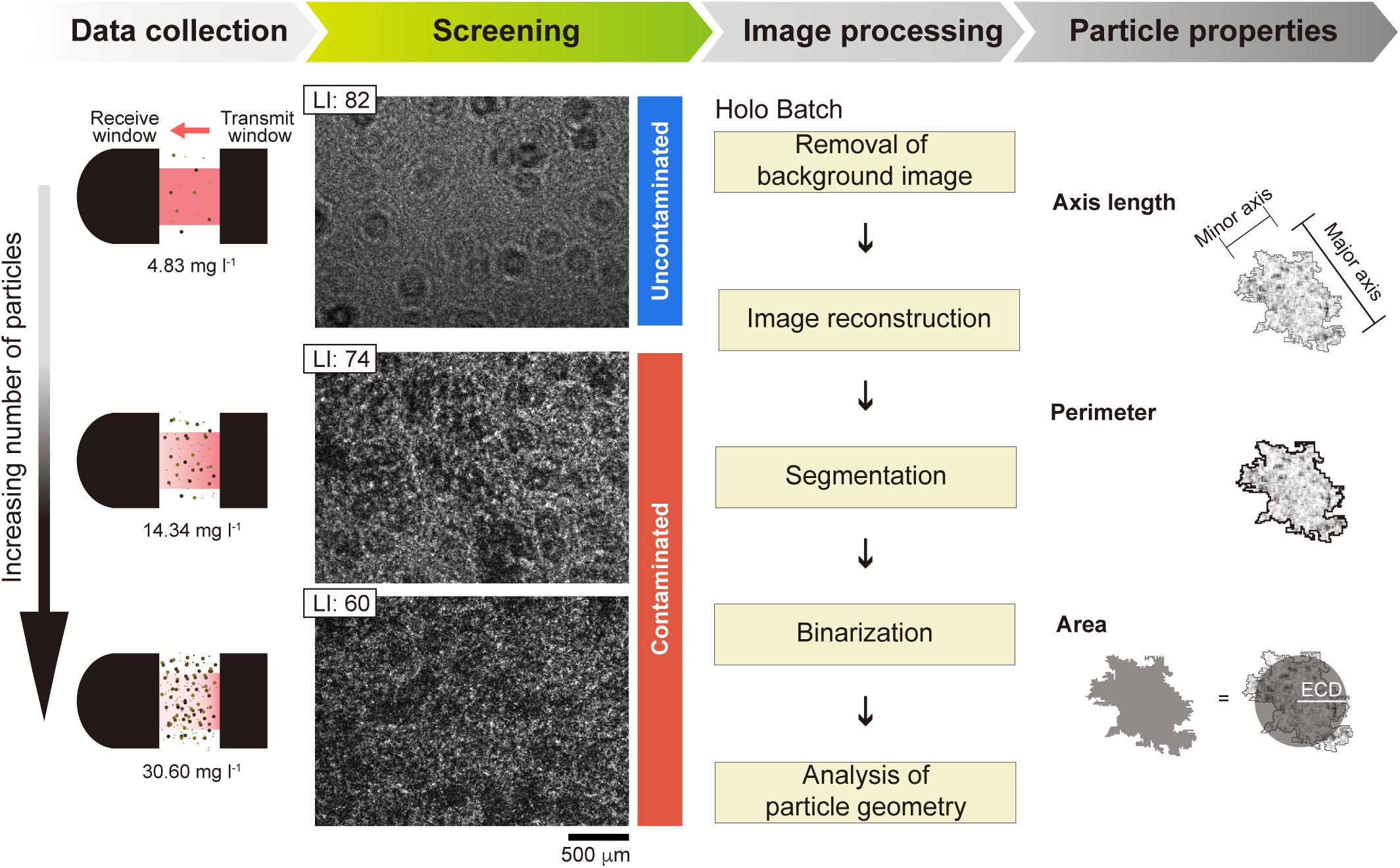
Figure 2. Conceptual flow chart for hologram image analysis (modified after Many et al., 2019). Light intensity (LI) normalized on a gray scale of 0 (black) to 255 (white) can be a reliable criterion for defining the contamination boundary. The holograms follow sequential steps to generate the Euclidean geometry of particles such as axis length, perimeter, area, and equivalent circular diameter (ECD).

Results and Discussion

Light Intensity as a Practical Criterion

In image processing for extracting particle properties, the evaluation of whether a hologram is contaminated is relatively subjective; further, the definition of the criterion for determining the contamination is not clear. This is because hologram contamination is primarily related to out-of-range SSC (i.e., SSC lower than the lower limit or higher than the upper limit of the instrument) during LISST-Holo measurements (Zhao et al., 2018). A critical SSC that generates mosaic patterns on a hologram depends on the particle size and beam attenuation with path length, as follows (Agrawal et al., 2008):

$c=-\ln t/L(1)$

$SSC=c\times d_{50}/1.13(2)$

where c is the beam attenuation coefficient (m^–1), t is the optical transmission (0.8), and L is the path length (m). The maximum SSC, in which the LISST-Holo captures a hologram with identifiable concentric rings, has a wide range from 8 to 16,456 mg l^–1 (Table 2; Sequoia, 2014). Because finer particles increase the beam scattering, the measurable range of SSC greatly decreases according to the reduced optical transmission (Agrawal et al., 2008). For the GTF and GRE, the identification of the concentric rings on the hologram distinctly varied depending on the SSC variability. Because the d₅₀’s of bed sediments at both sites were 17.5 (medium silt) and 30.7 μm (coarse silt), respectively, and L was fixed at 10 mm (see the shaded column in Table 2), the theoretical SSCs that the LISST-Holo would be able to measure were 308 and 617 mg l^–1 for GTF and GRE, respectively (Table 2). Both theoretical values were high enough to cover in situ SSCs measured at GTF (53–221 mg l⁻¹) and GRE (2–45.3 mg l^–1) without any hologram contamination.

TABLE 2

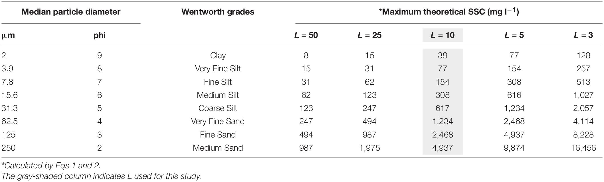
Table 2. Maximum theoretical suspended sediment concentration (SSC) as a function of particle size and sample path length (L) of LISST-Holo.

The LISST-Holo detected different sized particles ranging from 19.7 to 261.8 μm in GTF and GRE (Figure 3A). However, the distributions of d₅₀ decreased logarithmically as SSC increased. The d₅₀ eventually converged to approximately 30 μm above a specific SSC (GTF: 150 mg l^–1; GRE 30 mg l^–1). This made it appear as if only suspended sediments of uniform particle size existed in high-SSC conditions (see Supplementary Figure 1 for laboratory results). Even though the SSCs for GTF and GRE did not exceed the maximum theoretical SSC (Table 2), the holograms at SSCs above 69.9 (GTF) and 14.3 mg l^–1 (GRE) already included the mosaic patterns not suitable for image processing (see the holograms in Figure 2). This suggests that the actual upper limit of SSC may have differed from the maximum theoretical SSC because of the various local sediment properties (e.g., particle shape and composition) (Andrews et al., 2010; Graham et al., 2012). Such contradictory results between theoretical and actual conditions made it difficult to distinguish whether the hologram was contaminated. On the other hands, the LIs were similarly modulated in the range of 40–100, despite the difference in SSCs between GTF and GRE (Figure 3B). As the LI decreased (i.e., SSC increased), the d₅₀ for GTF and GRE also decreased to converge toward approximately 30 μm (see Supplementary Figure 1 for laboratory results). Unlike the maximum theoretical SSC that depends on local sediment characteristics, the LI allowed quantitative comparison of the overlapping degree of the concentric rings. The LI represents how intense (or dark) the gray shade of concentric rings is on a gray scale (Nakadate, 1986). Whether the hologram is contaminated is determined by the distinguishability of its interference patterns (concentric rings). In low-SSC conditions, for instance, concentric rings separated by certain distance from others can be identified. As the SSC increased, the overlap of bright and dark areas between the concentric rings limited the separation of the individual rings. This turned the hologram into a dark mosaic plane, which was a hindrance to detect particles with high accuracy (Murata and Yasuda, 2000).

FIGURE 3

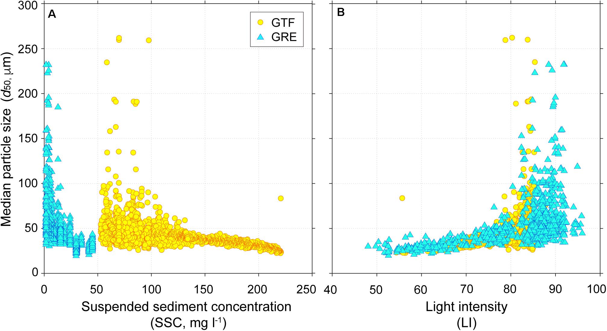
Figure 3. Variations in median particle size (d₅₀) by (A) suspended sediment concentration (SSC) and (B) light intensity (LI).

Particle Properties Distorted by Contaminated Holograms

Many concentric rings with different fringe spacings were produced on the holograms at the GTF and GRE. Following the procedure presented in Figure 2, each hologram including spatially incoherent particles within a sample volume was reconstructed at in-focused planes with an interval of 0.5 mm. The montage of the particles from the planes was visualized in the reconstructed image (file extension name: tiff) (Figure 4). For the GTF and GRE, the number of particles counted in the reconstructed images was in the range of 0–1,800 (Figure 5). In uncontaminated holograms with LI > 80, particles of less than 1,000 were reconstructed. As the LI decreased from 80 to 70, however, the number of particles with small A of 199.4–386.7 μm² abruptly increased, as shown in Figure 4. Their number, consequently, had reached up to 1,800 at LI = 70 with increasing SSCs to 191.7 (GTF) and 45.3 mg l^–1 (GRE). While LI decreased from 70 to 40, the number of particles approached nearly zero, even though the SSCs still increased. Considering the mosaic pattern on holograms with LI < 80 (Figures 4C–F), an abnormally large number of particles was derived from contamination. This is because the excessive number of suspended particles in the sample volume caused the concentric rings to overlap with each other (Brunnhofer et al., 2020). Therefore, the possibility of false extraction of particle properties on the reconstructed image was enhanced, resulting in increasing the number of small particles.

FIGURE 4

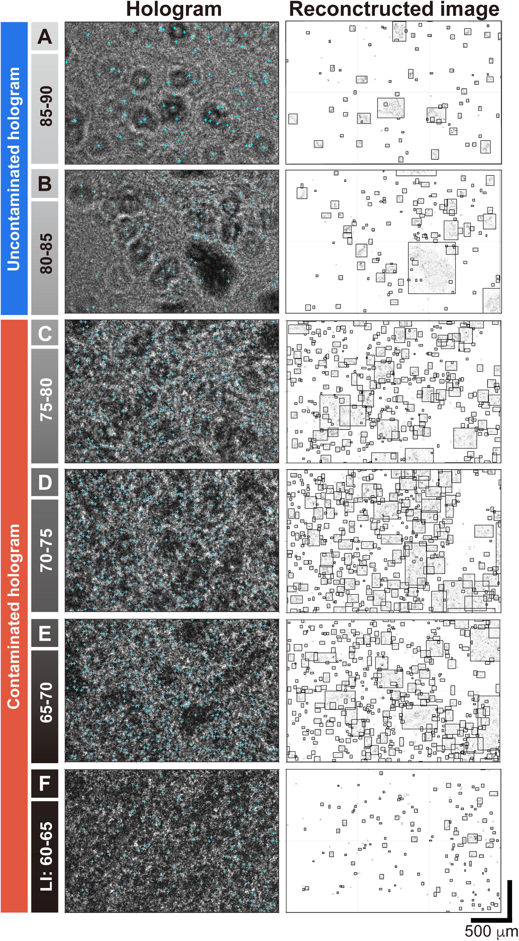
Figure 4. Representative holograms (left) and montages of reconstructed images (right) with different LIs. Cyan crosses on the hologram denote the centroids of particle area. Black bounding boxes on the reconstructed images exhibit the smallest area containing individual particles. Based on the LI, the holograms can be classified into uncontaminated [concentric rings, (A,B)] and contaminated [mosaic patterns, (C–F)].

FIGURE 5

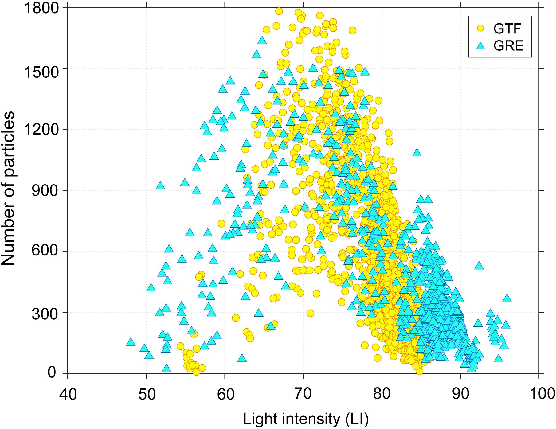
Figure 5. Changes in the number of particles under the various LI conditions.

For GTF and GRE, the particle size distribution (PSD) extracted from the contaminated hologram (LI < 80) had a positive skewness with d₅₀ of 30 μm (Figures 6A,B). The silt-sized particles lower than 64 μm accounted for approximately 96% (GTF) and 93% (GRE). As LI increased, the shape of the PSD shifted from a positively skewed (d₅₀ = 30 μm) to a normal distribution (d₅₀ = 56 μm). When LI was higher than 80, for GTF and GRE, the population of particles less than 64 μm decreased to account for approximately 61% and 46%, respectively, and the d₅₀ increased to 48.2 and 63.3 μm, respectively (see Supplementary Figure 2 for laboratory results). Moreover, the particle shapes (e.g., A and P) visualized in the reconstructed image were distorted (Figure 6C). Such particle shapes are usually represented as a combination of monochrome pixels in the reconstructed image. Furthermore, it was found that fine particles developed into irregularly shaped particles through flocculation. The cross-section of the particles had an uneven arrangement of pixels within A in the range of 279–1,305.1 μm². Depending on the local properties of bed sediments, the P of GRE was approximately 1.47 times higher than that of GTF in the equivalent particle area, because of the elongated or irregular shape by more flocculation. The A at GTF and GRE was greatly reduced to 423.2 and 400.8 μm², respectively, owing to the generation of 30 μm-sized distorted particles as the LI decreased. Meanwhile, P was slightly higher (approximately 10 μm) compared to the particles of equivalent A on uncontaminated holograms, leading to an increase in particle irregularity.

FIGURE 6

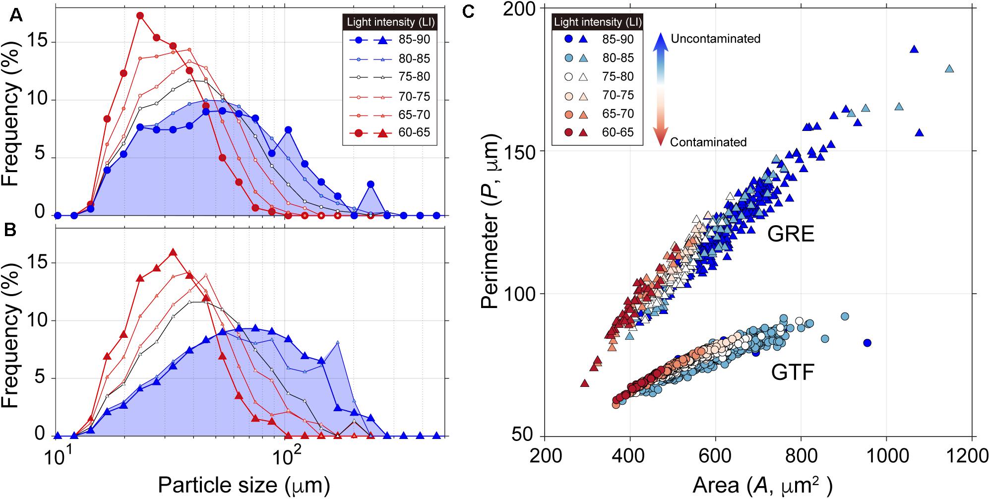
Figure 6. Particle size distribution (PSD) at (A) GTF (circles) and (B) GRE (triangles) under various LI conditions. (C) Relationship between perimeter and area of particles. Note that the PSD shifted from the positively skewed to normal distribution (blue shaded area for LI: 80–90), as the LI increased. The particles with smaller area and longer perimeters were mostly measured from the contaminated holograms.

Implications for Cohesive Sediment Transport

Contaminated holograms with distorted properties should be screened to derive accurate particle properties. In general, the three-dimensional structures of flocs expressed as a shape factor (e.g., A and P) of particles are irregular because of the repetitive flocculation and breakage (Jarvis et al., 2005; Maggi, 2013). In sediment dynamics, the shape factor is essential to determine the irregularity and settling velocity (W_s) of particles using the following equations (Maggi, 2007):

$D{F}_p=2\frac{\text{log}(P)}{\text{log}(A)}(3)$

$D{F}_{3D}=-1.63D{F}_p+4.6(4)$

$W_s=\frac{a}{18b}\frac{\left({\mathrm{\rho }}_p-{\mathrm{\rho }}_w\right)g}{\mathrm{\mu }}{d}_p^{3-D{F}_{3D}}\frac{d_f^{D{F}_{3D}-\mathrm{\hspace{0.33em}1}}}{1+0.15R^{0.687}}(5)$

where the perimeter-based fractal dimension (DF_p), modulated in the range of 1 (sphericity) to 2 (irregularity), is derived based on the relationship between A and P of individual flocs under the assumption of A = P^2/DFp (Maggi and Winterwerp, 2004). In Eq. 4, three-dimensional fractal dimension (DF_3D) is calculated in the range of 1.34 (irregularity) to 2.97 (sphericity) according to the DF_p (Lee and Kramer, 2004; Many et al., 2019). The ratio of a and b indicates the eccentricity of particles, ρ_p denotes the density of the primary particle (2,650 kg m^–3), μ is the dynamic viscosity of seawater (1.08 × 10^–3 Pa s), g is the gravitational acceleration (9.81 m s^–2), d_p is the primary particle diameter (1 μm), d_f is the floc diameter (μm), and R is the floc Reynolds number [R = W_s × d_f/ν, where ν is the kinematic viscosity of seawater (1.05 × 10^–6 m^–2 s^–1)] (Winterwerp, 1998).

The DF_p was distributed in the range of 1.28–1.41 (GTF) and 1.45–1.54 (GRE) (Figure 7A). As the particle size and LI decreased, DF_p gradually increased. The DF_p derived from contaminated holograms was overestimated by up to 2% compared to that from uncontaminated holograms (see Supplementary Figure 3 for laboratory results). Because the irregular shape of flocs resulted from flocculation, the distorted particles appeared to be highly flocculated compared to normal particles. This can be further extended to the subsequent determination of W_s which is essential to predict settling flux of fine sediments (Figure 7B). The irregularity of the floc shape normally contributes to the drag force on the flow through the suspended particles (Dietrich, 1982; Vahedi and Gorczyca, 2011; Maggi, 2013). Compared to flocs with circular shapes, flocs with irregular shapes have a lower W_s (Droppo et al., 2005). As the distortion of floc size and shape for GTF and GRE was enhanced, W_s decreased by approximately 0.01–0.04 mm s^–1 (Figure 7B; see the Supplementary Figure 3 for laboratory results). This was an underestimation of W_s since the increase of SSC as a concomitant of the strong current velocities contaminated holograms. However, it could be misunderstood as the flocs being broken into smaller flocs or primary particles with lower W_s by the strong current velocities (Winterwerp et al., 2006). The contaminated holograms, therefore, should be properly screened using our proposed method to prevent confusion.

FIGURE 7

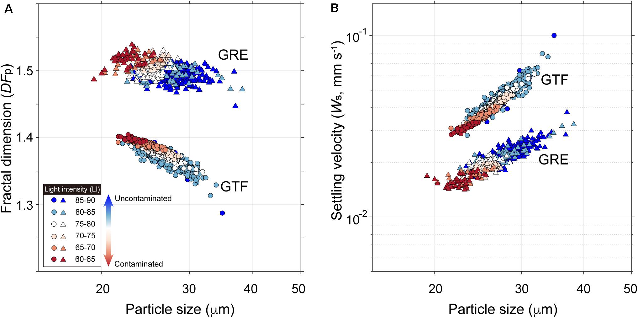
Figure 7. (A) Perimeter-based fractal dimension (DF_p) and (B) settling velocity (W_s) determined by the particle size. Note that the W_s derived from the contaminated holograms was lower than that from the uncontaminated.

Limitations

The practical method proposed in this study can be applied before performing image processing in the workflow (see Figure 2). This work reduces the labor and time required to determine whether a hologram is contaminated. Using LI, nonetheless, itself has inherent uncertainties. The LI could increase, for example, if suspended particles within the sample volume move faster than the recommended speed (up to 0.5 m s^–1) (Sequoia, 2014). Assuming that the particle moving velocity is close to the current velocity, a drastic increase in current velocity caused by natural forcing or artificial disturbances would lead to concentric rings of particles to be stretched. Such rings would appear as long bright lines along the trajectory of the particles, which could eventually increase the LI of the hologram.

The LI screening method is optimized for a high-SSC environment where frequent resuspension of cohesive sediments is observed. In offshore areas (e.g., Ha et al., 2015; Many et al., 2019), where the sediment supply is significantly limited, the possibility of hologram contamination caused by the overlapping concentric rings would be considerably low. In this case, the criterion of LI to screen the contamination might be higher than that proposed in this study. Therefore, the screening method requires additional post-processing (filtering and segmentation) suitable for each environment to extract the accurate particle information.

Conclusion

A practical method was proposed to screen holograms contaminated by overlapping interference patterns. The distorted particle properties of contaminated holograms were quantitatively estimated. The conclusions drawn from this study can be summarized as follows.

(1) The LI, which can be normalized on a gray scale of 0 (black) to 255 (white), is a reliable criterion for determining the contamination of holograms on the basis of the overlapping degree of concentric rings.

(2) Based on LI as a contamination boundary, the holograms were classified into contaminated images (LI < ca. 80) with mosaic patterns and uncontaminated images (LI > ca. 80) with identifiable concentric rings.

(3) The shape of the PSD shifted from a positively skewed to a normal distribution as the LI increased from the contaminated to uncontaminated holograms.

(4) Owing to the distortion of particle properties, the settling velocities derived from the contaminated holograms with mosaic patterns were underestimated compared to those derived from the uncontaminated holograms. Therefore, by screening the contamination, the proposed method can contribute to a more accurate estimation of the transport and behavior of cohesive sediments in shallow estuarine environments.

Data Availability Statement

The raw data supporting the conclusions of this article will be made available by the authors, without undue reservation.

Author Contributions

SC and JS conceived and designed the project, participated in data collection and processing, and wrote manuscript with contribution from all authors. GL and XS reviewed the manuscript. HH conceived and supervised the project and reviewed the manuscript. All authors contributed to the article and approved the submitted version.

Funding

The authors would like to acknowledge the funding support from the International Cooperation Program managed by the National Research Foundation of Korea (2020K2A9A2A06036472, FY2020), and the National Natural Science Foundation of China (51909068 and 52011540388). It was also supported by the project entitled “Development of Advanced Science and Technology for Marine Environmental Impact Assessment” (20210427), funded by the Ministry of Oceans and Fisheries of Korea (MOF).

Conflict of Interest

The authors declare that the research was conducted in the absence of any commercial or financial relationships that could be construed as a potential conflict of interest.

Supplementary Material

The Supplementary Material for this article can be found online at: https://www.frontiersin.org/articles/10.3389/fmars.2021.695510/full#supplementary-material

References

Agrawal, Y. C., Whitmire, A., Mikkelsen, O. A., and Pottsmith, H. C. (2008). Light scattering by random shaped particles and consequences on measuring suspended sediments by laser diffraction. J. Geophys. Res. Oceans 113:C04023. doi: 10.1029/2007JC004403

CrossRef Full Text | Google Scholar

Andrews, S., Nover, D., and Schladow, S. G. (2010). Using laser diffraction data to obtain accurate particle size distributions: the role of particle composition. Limnol. Oceanogr. Methods 8, 507–526. doi: 10.4319/lom.2010.8.507

CrossRef Full Text | Google Scholar

Brunnhofer, G., Hinterleitner, I., Bergmann, A., and Kraft, M. (2020). A comparison of different counting methods for a holographic particle counter: designs, validations and results. Sensors 20:3006. doi: 10.3390/s20103006

PubMed Abstract | CrossRef Full Text | Google Scholar

Choi, S. M., Seo, J. Y., Ha, H. K., and Lee, G. H. (2018). Estimating effective density of cohesive sediment using shape factors from holographic images. Estuar. Coast. Shelf Sci. 215, 144–151. doi: 10.1016/j.ecss.2018.10.008

CrossRef Full Text | Google Scholar

Davies, E. J., Buscombe, D., Graham, G. W., and Nimmo-Smith, W. A. M. (2015). Evaluating unsupervised methods to size and classify suspended particles using digital in-line holography. J. Atmos. Oceanic Technol. 32, 1241–1256. doi: 10.1175/JTECH-D-14-00157.1

CrossRef Full Text | Google Scholar

Davies-Colley, R. J., Ballantine, D. J., Elliott, S. H., Swales, A., Hughes, A. O., and Gall, M. P. (2014). Light attenuation-a more effective basis for the management of fine suspended sediment than mass concentration? Water Sci. Technol. 69, 1867–1874. doi: 10.2166/wst.2014.096

PubMed Abstract | CrossRef Full Text | Google Scholar

Dietrich, W. E. (1982). Settling velocity of natural particles. Water Res. Res. 18, 1615–1626. doi: 10.1029/WR018i006p01615

CrossRef Full Text | Google Scholar

Droppo, I. G., Nackaerts, K., Walling, D. E., and Williams, N. (2005). Can flocs and water stable soil aggregates be differentiated within fluvial systems? Catena 60, 1–18. doi: 10.1016/j.catena.2004.11.002

CrossRef Full Text | Google Scholar

Figueroa, S. M., Lee, G. H., and Shin, H. J. (2019). The effect of periodic stratification on floc size distribution and its tidal and vertical variability: Geum Estuary, South Korea. Mar. Geol. 412, 187–198. doi: 10.1016/j.margeo.2019.03.009

CrossRef Full Text | Google Scholar

Figueroa, S. M., Lee, G. H., and Shin, H. J. (2020). Effects of an estuarine dam on sediment flux mechanisms in a shallow, macrotidal estuary. Estuar. Coast. Shelf Sci. 238:106718. doi: 10.1016/j.ecss.2020.106718

CrossRef Full Text | Google Scholar

Gabor, D. (1948). A new microscopic principle. Nature 161, 777–778. doi: 10.1038/161777a0

PubMed Abstract | CrossRef Full Text | Google Scholar

Giering, S. L., Hosking, B., Briggs, N., and Iversen, M. H. (2020). The interpretation of particle size, shape, and carbon flux of marine particle images is strongly affected by the choice of particle detection algorithm. Front. Mar. Sci. 7:564. doi: 10.3389/fmars.2020.00564

CrossRef Full Text | Google Scholar

Graham, G. W., Davies, E. J., Nimmo-Smith, W. A. M., Bowers, D. G., and Braithwaite, K. M. (2012). Interpreting LISST-100X measurements of particles with complex shape using digital in-line holography. J. Geophys. Res. Oceans 117:C05034. doi: 10.1029/2011JC007613

CrossRef Full Text | Google Scholar

Graham, G. W., and Nimmo-Smith, W. A. M. (2010). The application of holography to the analysis of size and settling velocity of suspended cohesive sediments. Limnol. Oceanogr. Methods 8, 1–15. doi: 10.4319/lom.2010.8.1

CrossRef Full Text | Google Scholar

Ha, H. K., Kim, Y. H., Lee, H. J., Hwang, B., and Joo, H. M. (2015). Under-ice measurements of suspended particulate matters using ADCP and LISST-Holo. Ocean Sci. J. 50, 97–108. doi: 10.1007/s12601-015-0008-2

CrossRef Full Text | Google Scholar

Jarvis, P., Jefferson, B., and Parsons, S. A. (2005). Measuring floc structural characteristics. Rev. Environ. Sci. Biotechnol. 4, 1–18. doi: 10.1007/s11157-005-7092-1

CrossRef Full Text | Google Scholar

Katz, J., and Sheng, J. (2010). Applications of holography in fluid mechanics and particle dynamics. Annu. Rev. Fluid Mech. 42, 531–555. doi: 10.1146/ANNUREV-FLUID-121108-145508

CrossRef Full Text | Google Scholar

Kim, T. I., Choi, B. H., and Lee, S. W. (2006). Hydrodynamics and sedimentation induced by large-scale coastal developments in the Keum River Estuary, Korea. Estuar. Coast. Shelf Sci. 68, 515–528. doi: 10.1016/j.ecss.2006.03.003

CrossRef Full Text | Google Scholar

Lee, C., and Kramer, T. A. (2004). Prediction of three-dimensional fractal dimensions using the two-dimensional properties of fractal aggregates. Adv. Colloid Interface Sci. 112, 49–57. doi: 10.1016/j.cis.2004.07.001

PubMed Abstract | CrossRef Full Text | Google Scholar

Maggi, F. (2007). Variable fractal dimension: a major control for floc structure and flocculation kinematics of suspended cohesive sediment. J. Geophys. Res. Oceans 112:C07012. doi: 10.1029/2006JC003951

CrossRef Full Text | Google Scholar

Maggi, F. (2013). The settling velocity of mineral, biomineral, and biological particles and aggregates in water. J. Geophys. Res. Oceans 118, 2118–2132. doi: 10.1002/jgrc.20086

CrossRef Full Text | Google Scholar

Maggi, F., and Winterwerp, J. C. (2004). Method for computing the three-dimensional capacity dimension from two-dimensional projections of fractal aggregates. Phys. Rev. E Stat. Nonlin. Soft. Matter Phys. 69(Pt 1):011405. doi: 10.1103/PhysRevE.69.011405

PubMed Abstract | CrossRef Full Text | Google Scholar

Many, G., de Madron, X. D., Verney, R., Bourin, F., Renosh, P. R., Jourdin, F., et al. (2019). Geometry, fractal dimension and settling velocity of flocs during flooding conditions in the Rhônee ROFI. Estuar. Coast. Shelf Sci. 219, 1–13. doi: 10.1016/j.ecss.2019.01.017

CrossRef Full Text | Google Scholar

Merten, G. H., Capel, P. D., and Minella, J. P. (2014). Effects of suspended sediment concentration and grain size on three optical turbidity sensors. J. Soils Sedim. 14, 1235–1241. doi: 10.1007/s11368-013-0813-0

CrossRef Full Text | Google Scholar

Mills, G. A., and Yamaguchi, I. (2005). Effects of quantization in phase-shifting digital holography. Appl. Opt. 44, 1216–1225. doi: 10.1364/AO.44.001216

PubMed Abstract | CrossRef Full Text | Google Scholar

Ministry of Oceans and Fisheries (2019). Investigation of Hydrodynamic Variability in Geum River estuary. Final Report. Sejong-si: Ministry of Oceans and Fisheries, 700.

Google Scholar

Murata, S., and Yasuda, N. (2000). Potential of digital holography in particle measurement. Opt. Laser Technol. 32, 567–574. doi: 10.1016/S0030-3992(00)00088-8

CrossRef Full Text | Google Scholar

Nakadate, S. (1986). Vibration measurement using phase-shifting time-average holographic interferometry. Appl. Opt. 25, 4155–4161. doi: 10.1364/AO.25.004155

PubMed Abstract | CrossRef Full Text | Google Scholar

Nayak, A. R., Malkiel, E., McFarland, M. N., Twardowski, M. S., and Sullivan, J. M. (2021). A review of holography in the aquatic sciences: in situ characterization of particles, plankton, and small scale biophysical interactions. Front. Mar. Sci. 7:1256. doi: 10.3389/fmars.2020.572147

CrossRef Full Text | Google Scholar

Nayak, A. R., McFarland, M. N., Twardowski, M. S., Sullivan, J. M., Moore, T. S., and Dalgleish, F. R. (2019). “Using digital holography to characterize thin layers and harmful algal blooms in aquatic environments,” in Proceedings of the Digital Holography and Three-Dimensional Imaging, (Bordeaux: Optical Society of America). doi: 10.1364/DH.2019.Th4A.4

CrossRef Full Text | Google Scholar

Olson, E. (2011). Particle shape factors and their use in image analysis-Part 1: theory. J. GXP Compl. 15:85.

Google Scholar

Owen, R. B., and Zozulya, A. A. (2000). In-line digital holographic sensor for monitoring and characterizing marine particulates. Opt. Eng. 39, 2187–2197. doi: 10.1117/1.1305542

CrossRef Full Text | Google Scholar

Sequoia (2014). LISST-HOLO User’s Guide. Bellevue, WA: Sequoia Scientific Inc, 73.

Google Scholar

Sun, H., Dong, H., Player, M. A., Watson, J., Paterson, D. M., and Perkins, R. (2002). In-line digital video holography for the study of erosion processes in sediments. Meas. Sci. Technol. 13, L7–L12. doi: 10.1088/0957-0233/13/10/101

CrossRef Full Text | Google Scholar

Vahedi, A., and Gorczyca, B. (2011). Application of fractal dimensions to study the structure of flocs formed in lime softening process. Water Res. 45, 545–556. doi: 10.1016/j.watres.2010.09.014

PubMed Abstract | CrossRef Full Text | Google Scholar

Winterwerp, J. C. (1998). A simple model for turbulence induced flocculation of cohesive sediment. J. Hydraul. Res. 36, 309–326. doi: 10.1080/00221689809498621

CrossRef Full Text | Google Scholar

Winterwerp, J. C., Manning, A. J., Martens, C., De Mulder, T., and Vanlede, J. (2006). A heuristic formula for turbulence-induced flocculation of cohesive sediment. Estuar. Coast. Shelf Sci. 68, 195–207. doi: 10.1016/j.ecss.2006.02.003

CrossRef Full Text | Google Scholar

Woo, H. J., and Je, J. G. (2002). Changes of sedimentary environments in the southern tidal flat of Kanghwa island (Korean ed.). Ocean Polar Res. 24, 331–343. doi: 10.4217/OPR.2002.24.4.331

CrossRef Full Text | Google Scholar

Zhao, L., Boufadel, M. C., King, T., Robinson, B., Conmy, R., and Lee, K. (2018). Impact of particle concentration and out-of-range sizes on the measurements of the LISST. Meas. Sci. Technol. 29:055302. doi: 10.1088/1361-6501/aab83d

CrossRef Full Text | Google Scholar