 Mingshuai Sun
 Xianyong Zhao4
 Yancong Cai
 Kui Zhang
94% of researchers rate our articles as excellent or good
Learn more about the work of our research integrity team to safeguard the quality of each article we publish.
Find out more
ORIGINAL RESEARCH article
Front. Mar. Sci. , 09 June 2021
Sec. Marine Fisheries, Aquaculture and Living Resources
Volume 8 - 2021 | https://doi.org/10.3389/fmars.2021.693950
This article is part of the Research Topic Toward an Integrated Understanding of Ecological Responses to Variable Climate Changes and Marine Environments View all 9 articles
The objective of this research is to explore the relationships among various multidimensional factor groups and the density of fishery resources of ecosystems in offshore waters and to expand the application of deep machine learning algorithm in this field. Based on XGBoost and random forest algorithms, we first conducted regulatory importance ranking analysis on the time factor, space factor, acoustic technology factor, abiotic factor, and acoustic density of offshore fishery resources in the South China Sea. Based on these analyses, data slicing is carried out for multiple factors and acoustic density, and the relationship between multidimensional factor group and the density of marine living resources in the ecosystem of offshore waters is elaborately compared and analyzed. Importance ranking shows that the concentration of active silicate at 20 m depth, water depth, moon phase perfection, and the number of pulses per unit distance (Ping) are the first-order factors with a cumulative contribution rate of 50%. The comparative analysis shows that there are some complex relationships between the multidimensional factor group and the density of marine biological resources. Within a certain range, one factor strengthens the influence of another factor. When Si20 is in the range of 0–0.1, and the moon-phase perfection is in the range of 0.3–1, both Si20 and moon-phase perfection strengthened the positive influence of water depth on the density of fishery biological resources.
Long term monitoring data can be a good judgment of trends in fishery resources. A trend of degradation is observed in the coastal ecosystem, and the ecological problems such as the low age of fishery organisms, the miniaturization of individuals, and the degradation of the trophic niche are intensified (Chen Z. Z. et al., 2006; Chen et al., 2008, 2011; Qiu, 2002). Regulatory details in the short term are highly desirable for low age organisms dominated ecosystems. From the perspective of adverse factors, short-lived species have stronger adaptability, and survival opportunities, and their adaptive response to environmental changes is more rapid, while long-lived species have lower adaptability due to longer generations and higher energy demand (Lauchlan and Nagelkerken, 2020). In the short term, in order to adapt to the environmental changes, marine organisms tend to concentrate in time and space, which is more conducive to survival and reproduction (Chen and Chen, 2020; Lauchlan and Nagelkerken, 2020). The community distribution in the coastal ecosystem may also show a high correlation with some ecological factors, which may deeply affect the community structure and the distribution density of marine living resources in the ecosystem in a short time.
At present, the impact of various ecological factors on marine organisms has been extensively researched, including factors (Qiu et al., 2010; Zhang et al., 2017; Doray et al., 2018; Selfati et al., 2019; Chen and Chen, 2020; Lauchlan and Nagelkerken, 2020; Ljungstrom et al., 2020; Lopez et al., 2020) such as nutrients, temperature, water depth, longitude and latitude, transparency, chlorophyll, etc. The nutrients mainly include active silicate, active phosphate, nitrate, nitrite, and ammonium salt in seawater, which are the main food of marine phytoplankton closely related to aquaculture development. Therefore, the study of nutrient elements is necessary for the routine investigation of seawater chemistry, and it indicates the fertility of seawater. In the low ridge area, the growth and reproduction of organisms are limited, and the density of biological resources is relatively low. Whereas in the fertile sea area, many organisms can live in groups, and the density of biological resources is relatively high. Our recent studies have shown that there is a regulatory correlation between the density of fishery biological resources and the concentrations of nitrite, nitrate, and phosphate in a single season (Sun et al., 2020).
Compared with conventional studies, innovation lies in increasing the number of types of ecological factors and using deep machine learning method to analyze multidimensional ecological factors synchronously. In addition to the conventional factors, some factors of short-term time series also have potential research value, such as the moon phase perfection (Imre and Boisclair, 2005; Ndobe et al., 2014; Perez et al., 2019) (i.e., the moon’s surplus and deficiency state), continuous-time (24 h), etc. In terms of experimental conditions, different conditions of equipment may also have potential impacts on the data analysis, such as the working frequency (kHz) of the investigation equipment and the number of pulses related to the speed of navigation (Ping). The reported models in the literature are linear (including generalized linear models), additive models (including generalized additive models), and complex models (including deep learning, deep machine learning, and others). In general, models vary greatly in their expressiveness (formula or graphical expression) and the goodness of fit. For example, the linear model has the best expressiveness; however, the goodness of fit is the least. The additive model is less expressive than the linear model; however, it has higher goodness of fit. The goodness of fit of the complex model is the highest; however, the expression ability is poor. Moreover, Pearson’s correlation coefficient, which reflects the strength of the linear correlation, can only reflect the one-to-one relationship, and cannot measure the many to one relationship. The XGBoost (eXtreme Gradient Boosting) (Chen et al., 2016) and Random Forests (Svetnik et al., 2003) are potential deep machine learning algorithms, which are widely used in different fields, such as image classification (Bosch et al., 2007), data analysis (Marmion et al., 2010; Chen et al., 2017; Lu et al., 2018), and information classification (Torlay et al., 2017). They are also used to evaluate the sensitivity of features and calculate the importance scores for influencing factors (Menze et al., 2009; Sun et al., 2020). In the present study, we integrated these two deep machine learning algorithms to fit the multidimensional ecological factors and the nautical area scattering coefficient (NASC) (Chen G. B. et al., 2006; Knudsen et al., 2006; Zhao et al., 2008; Sun et al., 2019), which reflects the density of marine fishery biological resources.
In order to explore the combination of ecological factors that are most likely to affect the community structure of the ecosystem, we used the same standard to compare the multiple ecological factors and analyzed the possible action mode of the combination of ecological factors on the ecosystem.
Acoustic data were collected using single boat bottom otter trawl (engine: 441 kW, gross tonnage: 242 t, length of boat: 36.8 m, width: 6.8 m) in the offshore of the Northern South China Sea, named Beiyu 60011, with a scientific fisheries portable echo sounder (70, 120, and 200 kHz; Figure 1). Sampling time is July to August 2014, October to November 2014, April to May 2015 (see Table 1).
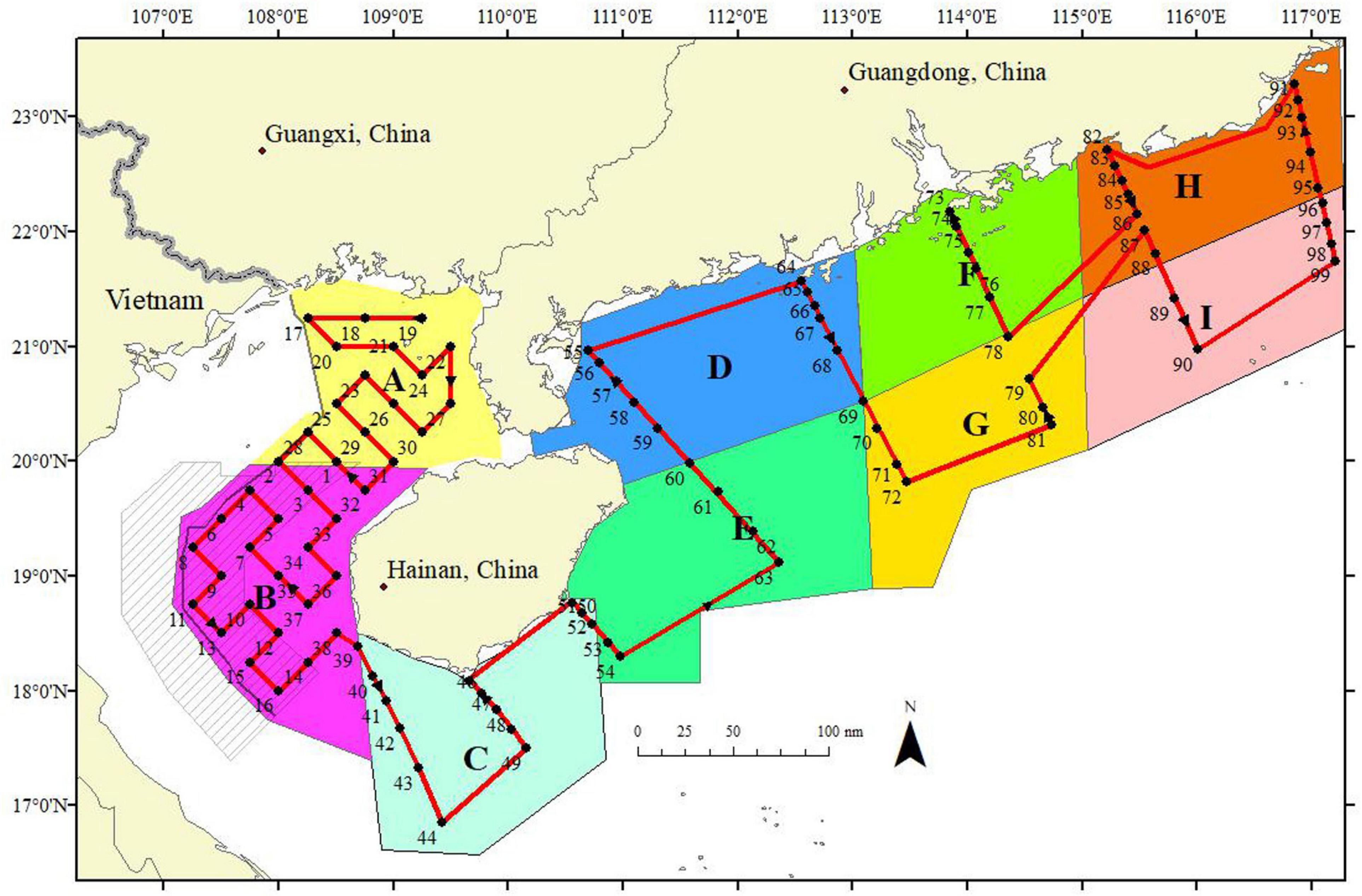
Figure 1. Acoustic navigation route (red lines) and sampling sites (black points) employed during the fishery. The letters A–I represent each partition (Map created in ArcGIS Desktop 9.3. https://www.esrichina.com.cn/).
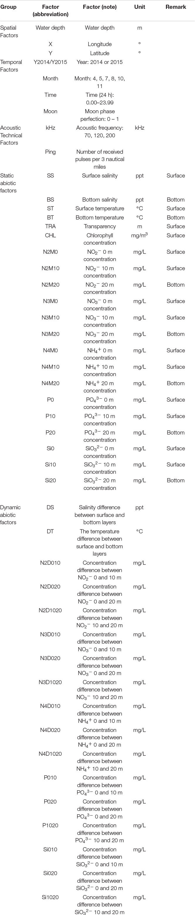
Table 1. List and grouping of all factors.
Fishery samples were collected from 99 sites using a single boat bottom otter trawls, with 404 type otter trawl, 80.80 m circumference, and 20 cm mesh size around the leading edge of the net. The total length of the net was 60.54 m, and the mesh size was 39 mm. It took 60 min per site. The sum mass and the number of samples were measured. The determination parameters of catches mainly include name, minimum body length and maximum length, minimum and maximum weight, total quantity and total weight.
Water temperature, salinity, and depth of water were obtained using AML Plus X, and nutrients and transparency were also collected. Both nutrient and transparency sampling methods use standard ocean survey sampling methods. The sampling depths for nutrients were 0, 10, and 20 m.
Echoview software (Version 6.11) was used for the analysis of the acoustic data. All data were checked carefully, and data not belonging to the routes were excluded. Data from two water layers were analyzed in the surface mixed layer (20 m below effective acoustic data line, except for blind zone) and the bottom cold-water layer (20 m above effective acoustic data line, except for blind zone). The basic integral voyage unit was selected as 3 nmi. The integral threshold was set as −80 dB. Background noise was removed, and the surface and bottom NASC (m2/nmi2) integral values were collected, which were also fishery density for the same volume as the sampling range for surface and bottom cold-water layers was the same. NASC-based fisheries acoustics technology has been widely used in the field of fishery resources assessment (Maclennan and Holliday, 1996; Mason et al., 2005; Simmonds and Maclennan, 2005).
Abiotic factors included both primary and derived. Primary features include surface salinity (SS, ppt) and surface temperature (ST, °C) at 2 m in the surface mixed layer, bottom salinity (BS, ppt) and bottom temperature (BT, °C) at 2 m in the bottom cold water layer, water depth (WD, m), longitude (X, °), latitude (Y, °), time (24 h), year, month, moon-fullness ratio (moon), transparency (TRA, m), and chlorophyll concentration (CHL, mg/m3). The derived factors calculated on the basis of primary factors included salinity difference (DS, ppt) and temperature difference (DT,°C) between the surface and bottom cold-water layers, concentration difference between NO2– at 0 m and 10 m (N2-d010, mg/L), and a few others as given in Table 1.
The present study classified all factors into five categories: (1) spatial factors; (2) temporal factors; (3) acoustic technical factors; (4) dynamic abiotic factors or stressors, with all derived factor (total 17), and (5) the other 21 factors or stressors, belonging to the static abiotic factors. See Table 1 for details.
The sample size, an important part of the analysis on factors, was less than 100 in the offshore of the northern South China Sea in this study and was limited by the number of survey sites. As the sample size was not enough to analyze the data comprehensively, we extended point data to face data by spatial interpolation. Interpolation methods included Kriging and inverse distance weighting (IDW). The methods were selected based on the highest goodness of fit (R2) and minimum mean squared error (MSE) (Sun et al., 2019). The longitude and latitude of resampling were determined according to the acoustic navigation route, and the minimum distance between sampling points was three nautical miles. Abnormal data were screened and eliminated, and 2544 valid sample points were obtained.
The relationships between the NASC and the 48 factors were determined with XGBoost, Random Forests, and linear regression models. Furthermore, all the 48 factors sampled were made dimensionless using Min-Max Scaling (Normalization). The model effect was estimated based on the highest goodness of fit (R2) and MSE from cross-validation methods. The proportion between the training dataset and the testing dataset was 7:3. According to Zhou (2016), when the amount of data is small, about 2/3 to 4/5 of the sample data should be used for training, and the rest should be used for testing. Besides, a proportion of 7:3 of the training data and test data are also a kind of allocation ratio usually employed for small data, which can effectively improve the generalization ability of the model.
The XGBoost and random forests models are based on multiple decision trees on the same dataset. Random Forests model generates several trees, and each tree is independent (Svetnik et al., 2003) with leaves of equal weight within the model for obtaining higher accuracy. The XGBoost introduces leaf weighting to penalize those trees that do not improve the model predictability (Chen and Guestrin, 2016; Chen et al., 2016). In order to improve the efficiency of model optimization, some important parameters can be adjusted. If satisfactory results are achieved, model optimization is ended. If the results of model optimization are not satisfactory, fine adjustment of parameters that are more complex is carried out. Here, we adjusted the learning_rate, n_estimators, and the subsample (Chen and Guestrin, 2016). With the optimized model, feature weighting of the 48 factors on fishery resource density was calculated and their importance scores were obtained.
The analysis was performed in Python 3.7 using the Scikit-Learn package (Pedregosa et al., 2013) and the XGBoost library (Chen and Guestrin, 2016; Chen et al., 2016).
The analysis of the sensitivity of factors provides a score that indicates the value of each feature in the construction of decision trees within the model. In order to reduce the error, the importance scores for each factor in XGBoost and random forests were averaged. The sum contribution was set as 50, 80, and 95%, ranked from level one to level four, meaning the first level was the most important, and the fourth was the lowest.
The association between significant factors and density was comprehensively analyzed by Pearson’s correlation coefficient as well as multidimensional factor slicing.
The two regulatory deep machine learning algorithms (XGBoost and Random Forest) performed much better than the linear regression model. It is reflected in the differences of both goodness of fit (R2) and MSE values (Figure 2). Both XGBoost and Random Forests have advantages; however, the R2 of Random Forests is slightly higher, but the MSE of XGBoost is lower.
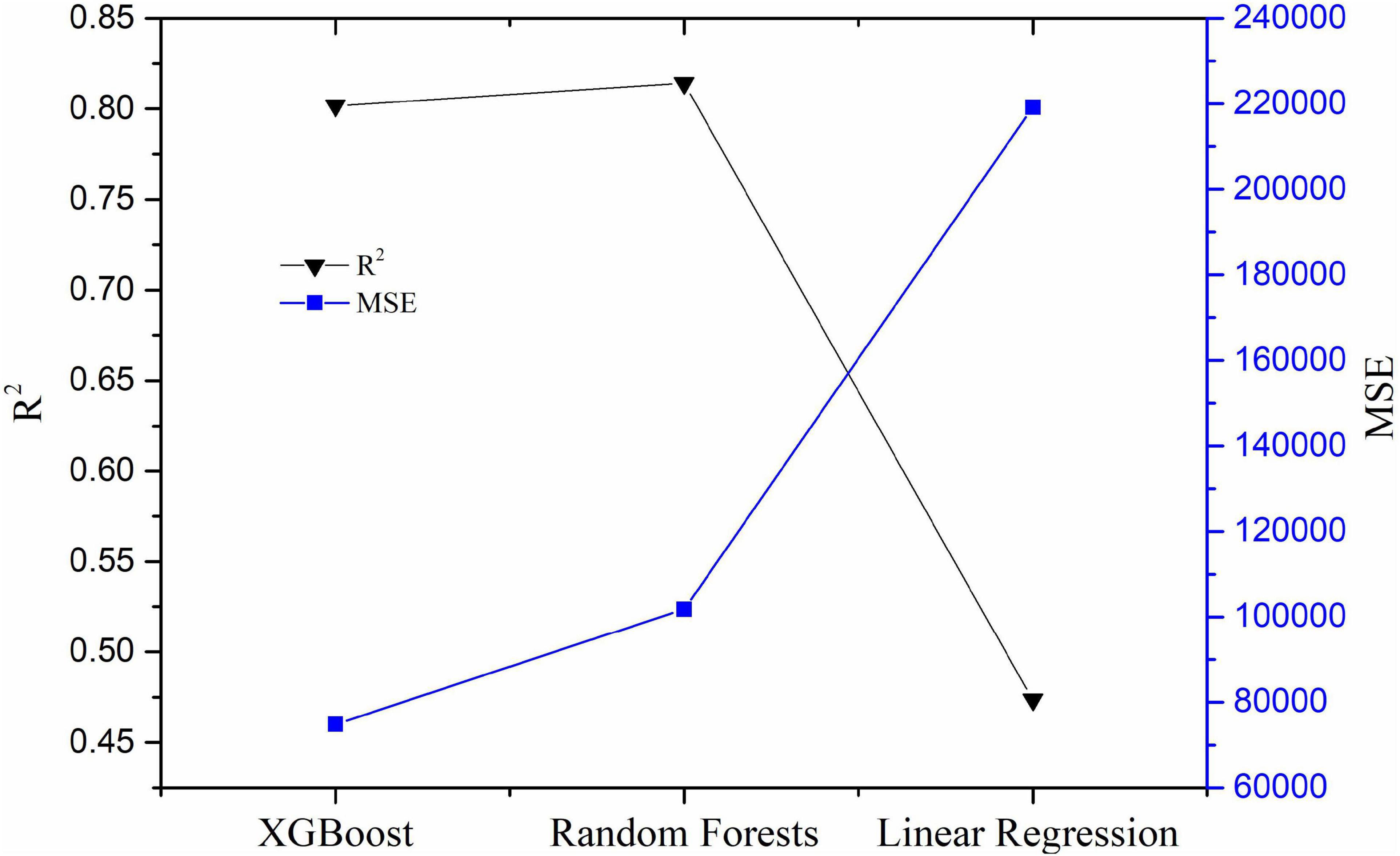
Figure 2. The comparison of the goodness of fit (R2) and mean squared error (MSE) of the three algorithms: the black inverted triangle represents R2, and the blue square is the MSE.
According to Figure 3, the total score of the first level factors affecting the density distribution of fishery resources is about 0.5 (characteristic contribution rate is 50%), which includes SiO32– 20 m concentration (Si20, mg/L), water depth (m), and moon phase perfection (moon, 0∼1). The importance score of SiO32– 20 m concentration (Si-20 m, mg/L) is 0.26 (characteristic contribution rate 26%), which is >0.20 and can be used as the maximum probability influencing factor. Water depth (m) with an importance score of 0.12 (characteristic contribution rate of 12%), which is >0.10 and is a large probability influencing factor. The total score of the second level factor is about 0.3, mainly including 21 factors, such as NO2– 0 m concentration (N2M0, mg/L), NH4+ 0 m concentration (N4M0, mg/L), SiO32– 10 m concentration (Si10, mg/L), time (24 h, 0.00–23.99), temperature above 2 m at the bottom (BT, °C), month (4–5, 7–8, 10–11), salinity above 2 m at the bottom (BS, PPT), the temperature difference between surface and bottom (DT, °C), longitude (X, °), chlorophyll (CHL, mg/m3), concentration difference of PO43– between 0 and 10 m (P010, mg/L), transparency (TRA, m), the concentration difference of NO2– between 0 and 20 m (N2D020, the concentration of NH4+ 20 m (N4M20, mg/L), and the concentration difference of NO3– between 0 and 20 m (N3D020, mg/L). The total score of the third level factor is about 0.15, including 16 factors such as temperature at 2 m of surface layer (ST, °C), NO2– 20 m concentration (N2M20, mg/L), PO43– 20 m concentration (P20, mg/L), salinity at 2 m of surface layer (SS, ppt), and so on (see Figure 3 for details). The total score of the fourth level factor is about 0.05, including 12 factors, which are the lowest group of importance scores, including the concentration difference of SiO32– between 0 and 10 m (Si010, mg/L), the concentration difference of SiO32– between 0 and 20 m (Si020, mg/L), and so on (see Figure 3 for details).
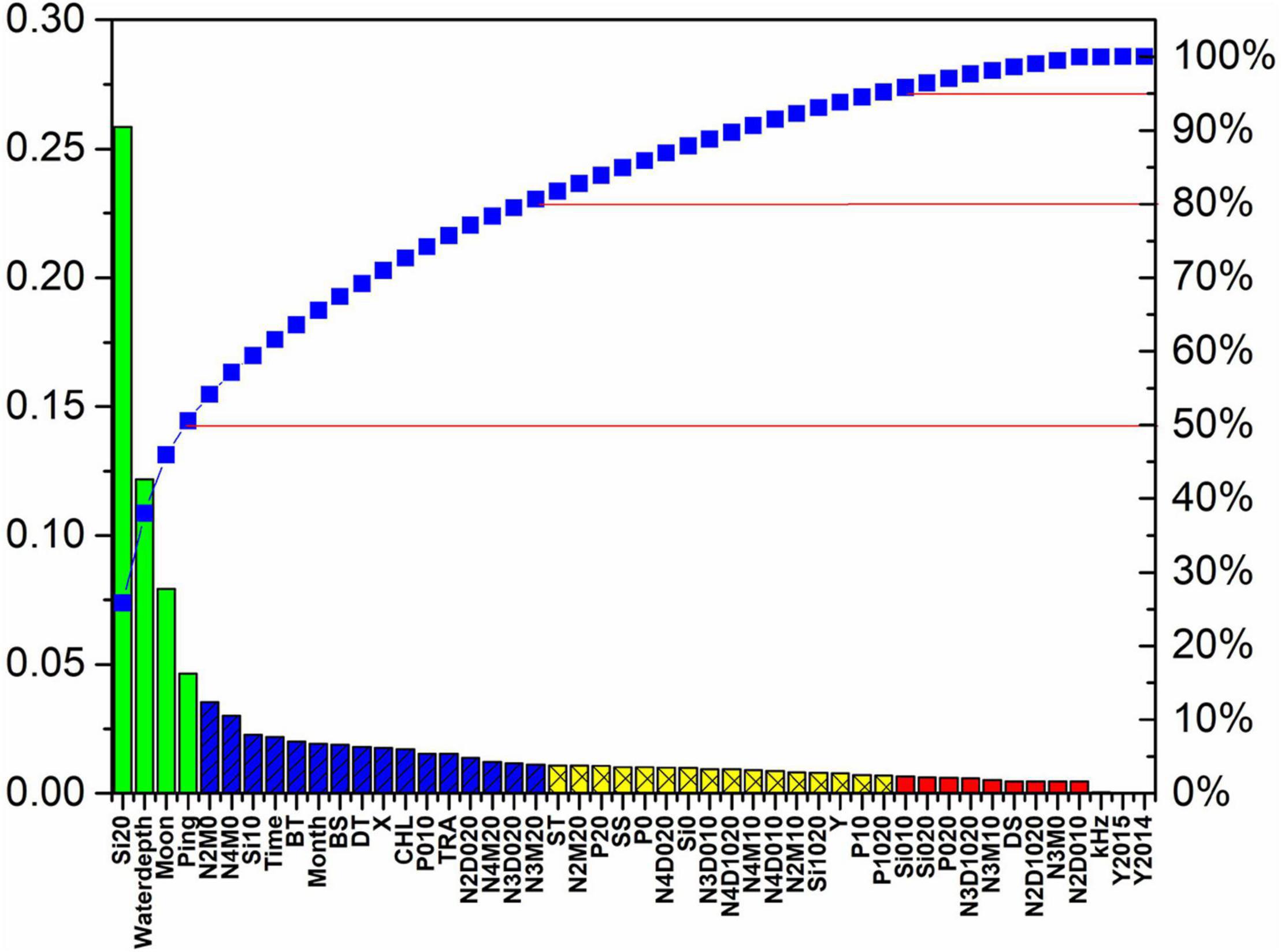
Figure 3. The comprehensive order of importance between the acoustic density of fishery resources and the 48 factors of five major categories in the offshore ecosystem of the South China Sea. Green, blue, yellow, and red represent the first level to the fourth level, respectively, and the cumulative contribution rate ranges are 50, 80, and 95%, respectively.
The total score represents the sum of the importance of all such factors, and the average represents the arithmetic mean of the importance of all such factors. The total score shows that the static abiotic factors ranked the highest (Figure 4), accounting for more than half of the importance, followed by the dynamic abiotic factors, spatial factors, temporal factors, and finally acoustic technical factors. The average score shows that spatial factors have the highest mean value, followed by the static abiotic factors, temporal factors, and acoustic technical factors, and finally, dynamic abiotic factors.
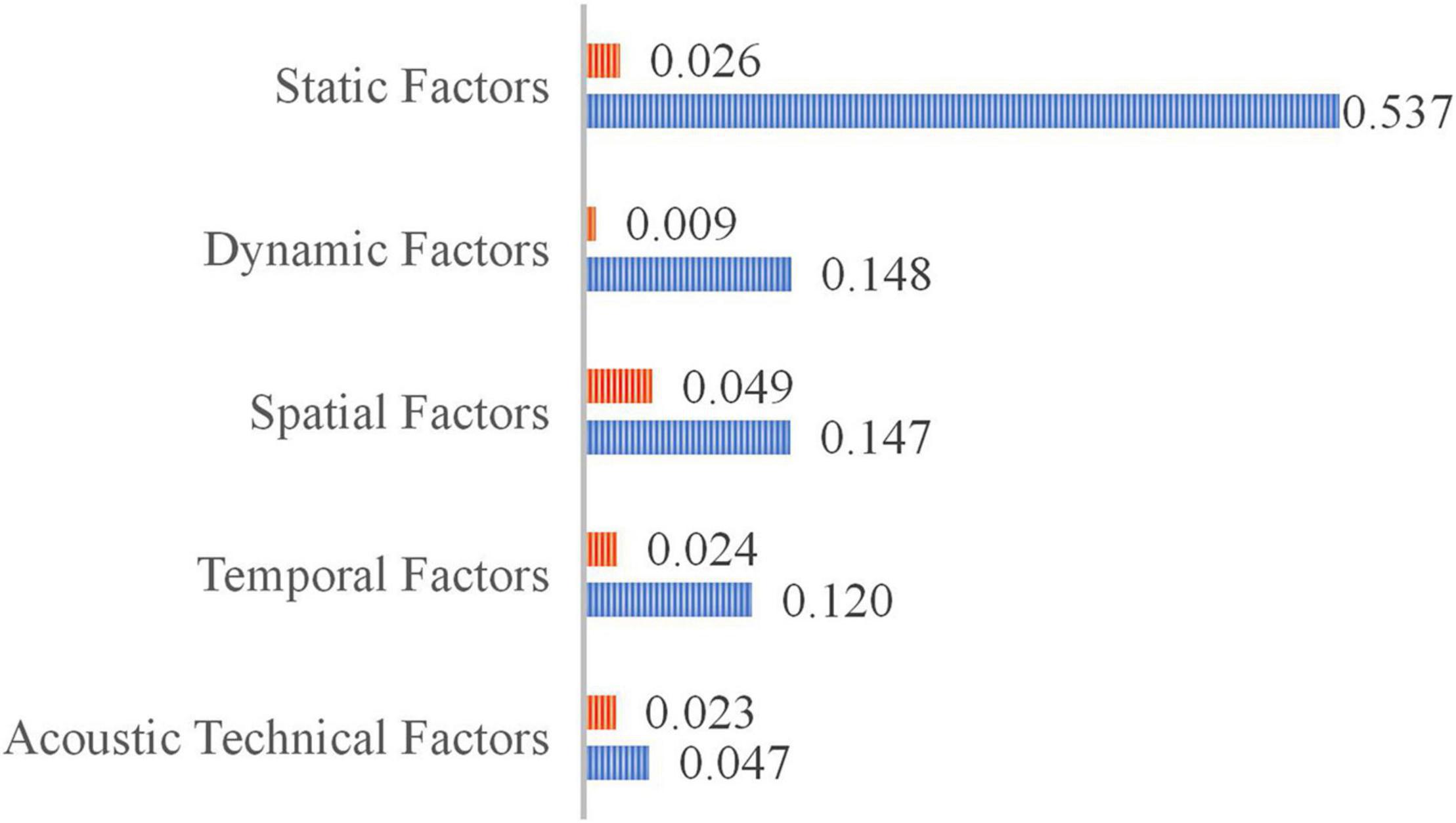
Figure 4. Comparison of the total score (blue stripe) and the average score (red stripe) of different categories of factors.
In the first level factor, static factor, spatial factor, temporal factor, and acoustic technical factor account for one share, respectively.
The first-order factors showing positive correlations with the NASC are water depth and Ping, and that showing a negative correlation is Si20 (Figure 5). However, there is only a very weak linear correlation between the NASC and the moon. The moon phase, which seems to be relatively independent, has a positive correlation with Si20 and Ping; however, the correlation with Si20 is slightly stronger than that with Ping. Therefore, moon phase perfection may act on both the negative and positive factors related to the NASC. Overall, the NASC is independent of water depths, while the other factors have certain internal relations, and the moon phase perfection may play a bi-directional balancing role in it.
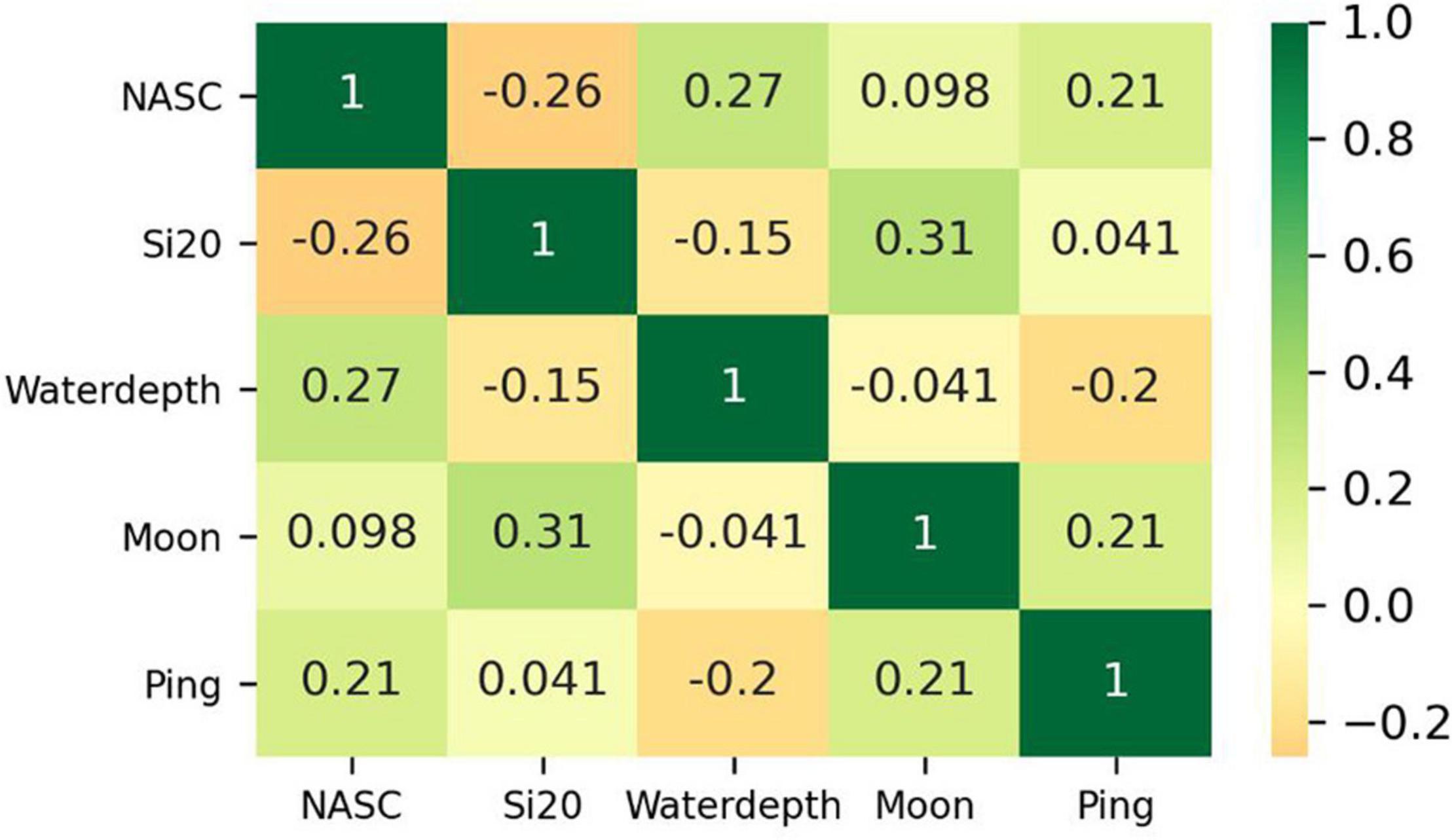
Figure 5. Pearson’s correlation matrix between the nautical area scattering coefficient (NASC) and the first-order factors.
The correlation characteristics between the NASC and the Si20 are different in different seasons (Figures 6–8 and Table 2). However, the correlations are similar for A, B, C, G, H, and I, in different seasons, in which the NASC and the Si20 are positively correlated for B, while the rest shows a negative correlation. The seasonal differences in the correlation between NASC and Si20 in D, E, and F regions are prominent.
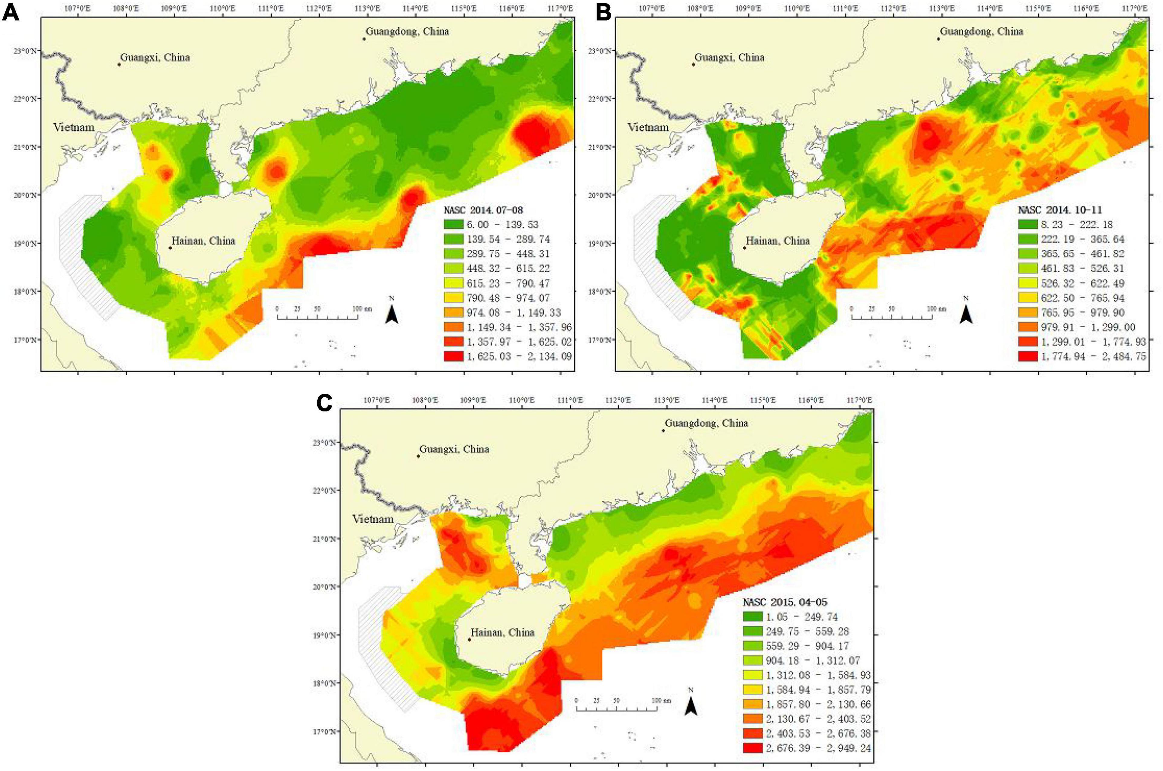
Figure 6. The temporal and spatial distribution of the nautical area scattering coefficient (NASC). The color green is the lowest, yellow is the middle, and red is the highest. (A) July to August 2014; (B) October to November 2014; (C) April to May 2015.
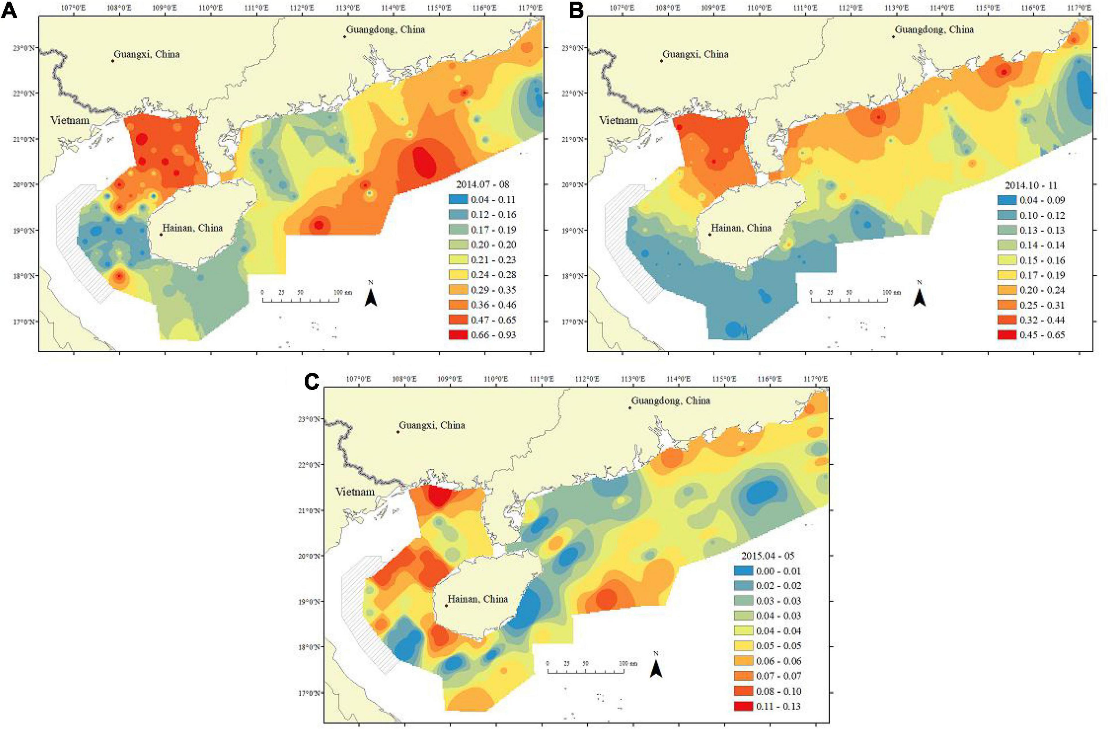
Figure 7. The temporal and spatial distribution of Silicates at 20 m depth (Si20). Blue is the lowest, yellow is the middle, and red is the highest. (A) July to August 2014; (B) October to November 2014; (C) April to May 2015.
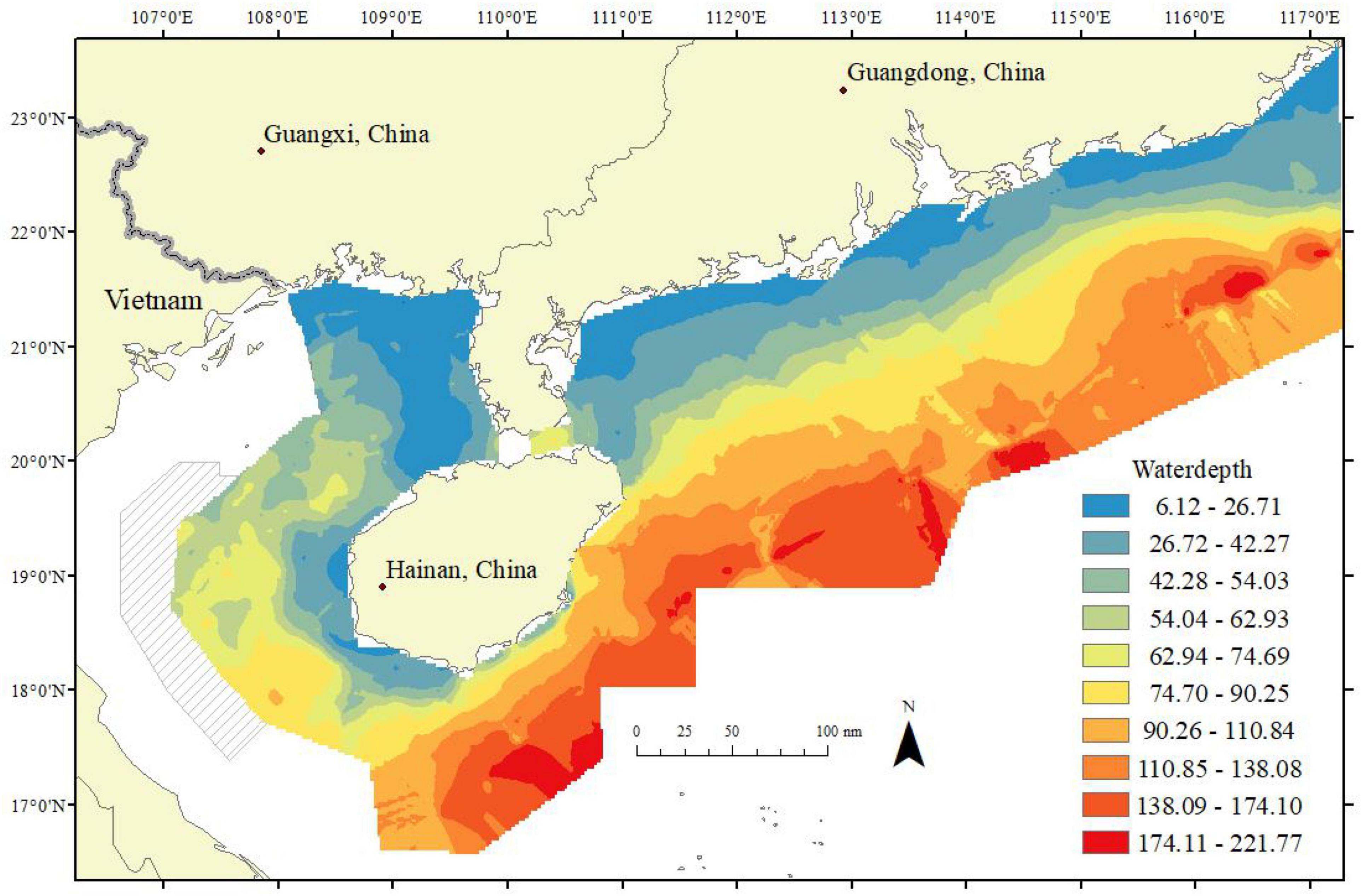
Figure 8. The spatial distribution characteristics of water depth measured by acoustic equipment: blue is the shallowest, yellow is the middle, and red is the deepest.
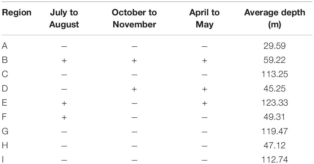
Table 2. The positive or negative correlations between the NASC and the Si20 values in different seasons in the A–I region.
The distribution curve of NASC is mainly in the range of 60–200 m2/nmi2, and there is no significant difference among different moon phase perfection (Figure 9). The distribution of Si20 is concentrated in the range of 0.12–0.20 mg/L during the moon of 0.0–0.3, and the distributions in other moon phases are gentle. There is no significant linear correlation in the scatter distribution map; however, different Y corresponding to the same variable X shows different scatter distribution patterns. For example, the scatter distribution is crescent, circular, and rectangular, when X is NASC and Y is Si20, water depth, and Ping, respectively. The distribution of dark color is more concentrated than that of the light color, which corresponds to each phase of the moon.
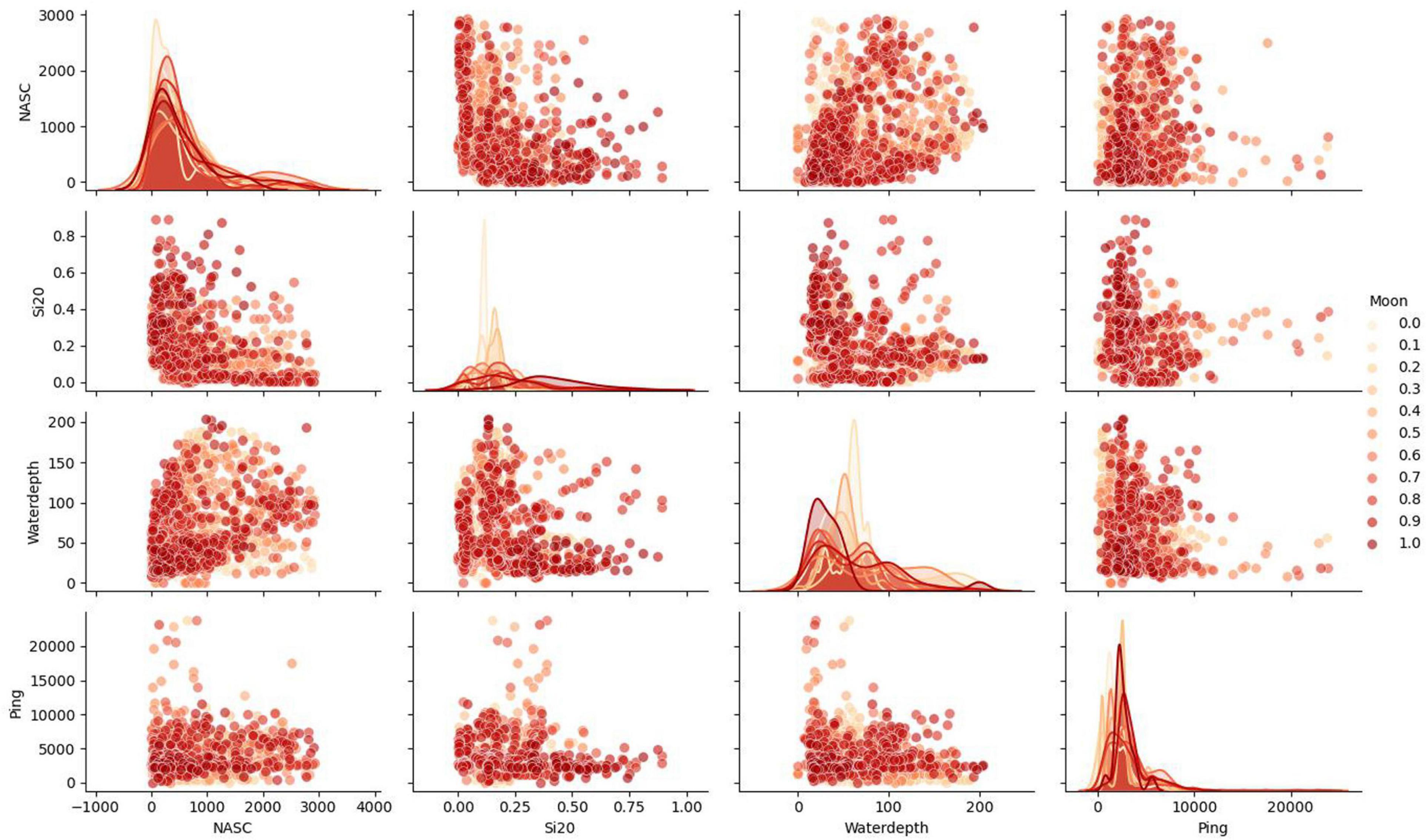
Figure 9. The scatter distribution of the nautical area scattering coefficient (NASC) and main factors, and the diagonal diagram is the distribution curve of each factor in different moon phase perfections. The color of the dot or line gradually deepens with the increase of the moon’s degree of fullness.
Multidimensional data provides more information and is more conducive to regulatory correlation analysis.
There are several interesting findings in Figure 10:
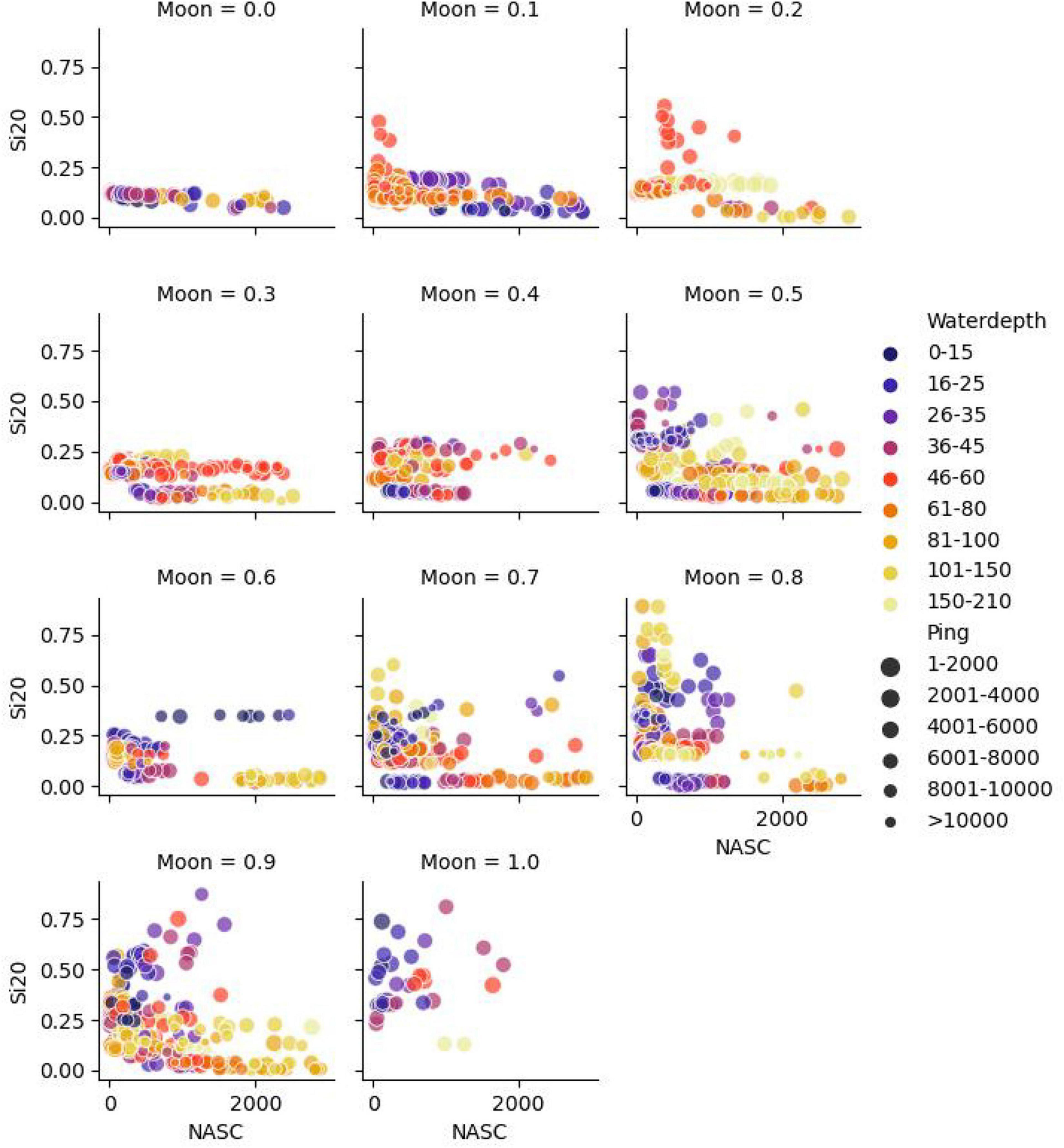
Figure 10. Scatter plot of multidimensional data: the color of the points distinguishes the water depth, and the size of the points distinguishes the number of Ping in each acoustic analysis unit.
(1) It seems that the moon phase perfection has an effect on the fluctuating range of Si20. In the 0.0–0.4 range of lunar phase, Si20 is relatively stable, of which only the phase 0.2 shows a small amount of continuous fluctuation within 0.1–0.6, and the fluctuation depth is about 60 m, and the corresponding abscissa NASC value is 500. In the 0.5–1.0 range of the lunar phase, Si20 fluctuates greatly, and the maximum water depth is mainly in the shallow water area (within 45 m) or the deep-water area (150–200 m). When the moon phase is 0.8, the fluctuation range is the largest, and the abscissa NASC is concentrated in the range of 0–500. When the moon phase is 0.9 and 1.0, NASC increases and disperses in the high-value range of Si20.
(2) When Si20 is close to 0, and the moon phase perfection is greater than or equal to 0.3, the NASC value shows a positive correlation with water depth; that is, the deeper the water depth, the greater the NASC value.
(3) ] When the moon phase perfections are0.2, 0.5, 0.7, 0.8, and 0.9, the correlation trend between Si20 and NASC is reversed.
(4) Higher the Ping value (the smaller the point, i.e., the lower the ship speed) shows a higher aggregation of points. When the moon is 0.5, 0.7, and 0.8, high Ping value clusters of Si20 and NASC appear in shallow water.
In this study, we used a deep machine learning algorithm to analyze the importance of five kinds of factors to NASC and further carried out multidimensional data analysis on several main factors. Some results are dialectically analyzed, including algorithms, factor categories, analysis strategies, relative relations and so on.
Compared with deep learning, deep machine learning focuses more on ensemble learning algorithms, such as XGBoost and Random Forests. Both models are machine learning algorithms with better performance (higher R2 and smaller MSE value) than the linear regression model under the condition that data quality and sample size are the same. Moreover, with the increase of data volume, the model performance also improves (Sun et al., 2020). Based on the interpolation methods, data size could be extended using coordinates (Burrough and Mcdonnel, 1999; Freeman and Moisen, 2007; Sales et al., 2007; Pereira et al., 2015; Sun et al., 2017) to improve the performance of deep machine learning algorithms.
Deep machine learning algorithm has a wide range of application potential and can be used for multi-domain and interdisciplinary comprehensive analysis. XGBoost and Random Forests are widely used in several areas, such as image classification (Bosch et al., 2007), data analysis (Marmion et al., 2010; Chen et al., 2017; Lu et al., 2018), and information classification (Torlay et al., 2017). They are also used to evaluate the sensitivity of features and calculate the importance scores for all factors (Menze et al., 2009; Sun et al., 2020). Through the goodness of fit (R2), MSE, and importance ranking of feature factors obtained using deep machine learning algorithm modeling; we can analyze and infer the relationship, which is difficult to find using linear functions. High goodness of fit and relatively small MSE indicate that the modeling performance is good, and the model has high credibility for data understanding and mining. The importance ranking of feature factors reflects the correlation strength of various factors on the acoustic density of marine fishery organisms in this study.
Instead of using the importance score of XGBoost or Random Forests separately, we used the average of the two methods. As XGBoost and Random Forests models have their own advantages and disadvantages (Pedregosa et al., 2013; Chen et al., 2016), in order to avoid the extreme of the two methods, we adopted a compromise approach. Besides XGBoost and Random Forests models, support vector machine (SVM) (Huang et al., 2014) and logistic regression (Cheng et al., 2006; Pal, 2012; Talenti et al., 2015) are available for feature selection. If a simple method can achieve good modeling results, it should be used first. However, most of the data often possess complex regulatory relations; therefore, deep machine learning often has better performance for research projects with a multidimensional and a large amount of data.
The factors related to the distribution of marine living resources are of many kinds. In the study, we mainly select five categories that can be divided into four categories, namely, spatial factors, temporal factors, acoustic technology factors, and physical and chemical factors. Among them, physical and chemical factors are divided into two categories, namely static abiotic factors and dynamic abiotic factors. Overall, 21 static abiotic factors, 17 dynamic abiotic factors, 5 temporal factors, 3 spatial factors, and 2 acoustic technical factors are used in this study.
It is observed that the static factor is the most important factor among the five categories and is related to a number of factors. Physical and chemical factors, also known as abiotic factors, are the various elements in the living environment of marine organisms that are the most directly related to the survival and distribution of marine organisms. There are many kinds of abiotic factors, and these factors in different horizontal or vertical positions may have different degrees of correlation with the survival of marine organisms. This correlation is closely related to the multidimensional ecological factors (Sun et al., 2020). The average importance score of dynamic physical and chemical factors is the lowest, which is similar to that of a single season (Sun et al., 2020). Therefore, the types of dynamic physical and chemical factors in the study can be appropriately reduced to simplify the composition of characteristic factors and improve modeling efficiency.
As the results of this paper show, the relationship between the distribution of marine organisms and multidimensional factors is complex and regulatory. The importance of the same factor in different time periods and different regions is different, which may be a positive correlation or a negative correlation. The average importance score of the spatial factor is the highest, and the average importance score of the temporal factor is the third, which indicates the necessity of comprehensive research on these two factors. Spatial factors are mainly used to measure some horizontal spatial characteristics, such as longitude, latitude, and water depth. The temporal factor is mainly used to quantify some variables with time characteristics, such as year, month, time, and moon phase perfection. There are few reports about the influence of the time and the moon phase on the density of marine living resources.
Different kinds of data have their own units of measurement, and for each of these factors, different acquisition methods or technical means may also have certain errors, which may hamper the research results. Therefore, acoustic technical parameters are taken as characteristic factors. These factors are several important parameters in the acoustic evaluation method of fishery resources and are related to the acquisition method of data. The factor “kHz” is used in this paper to evaluate the level of influence of different sound frequencies on the survey data (Brierley et al., 2004; Yasuma et al., 2006; Godlewska et al., 2009; Guillard et al., 2014; Garcia-Seoane et al., 2016). Another acoustic technical factor, Ping, evaluates the level to which navigation speed affects survey results. The result shows that the average importance score of acoustical technical factors is not the lowest among the five categories indicating that related technical factors may have some influence on the research results.
All kinds of factors are important nodes of the multidimensional network. Whether they are related to the survival and distribution of marine living resources, climate, and environmental factors, etc., they all have complex relationships. However, the difficulty of analysis increases with the dimension.
We have attempted to slice major factors, such as time or space factors, by selecting a factor or a class of factors as slicing angles. In the study, the temporal factor of the first-order factor, moon phase perfection, was used as the slicing angle for the multidimensional analysis.
It is worth considering the choice of model fitting and application ability. Increasing the time dimension may not necessarily improve the fitness of the model, rather reduce fitness. The multi-season fitting is about 80% and the single-season fitting is up to 94% (Sun et al., 2020); however, the generalization of the model is greatly limited. The reduction of time span makes the model only useful to analyze the relationship between existing data and loses the ability to predict future data. Therefore, a large time span may lose fitness; however, its ability to predict future data improves.
Targeted analysis based on known or possible features of the research object may have a better modeling performance. Ocean water bodies are layered cubic spaces, and marine life distributions vary from region to region, both in horizontal space (longitude and latitude) and vertical space (different water layers or depths). Therefore, stratified analysis of marine biological resource density is usually better than non-stratified analysis. The fitting degree of stratified analysis is 9–14 percentage points higher than that of non-stratified analysis (Sun et al., 2020). That is, the stratified feeding characteristics of the research object (marine organisms) can be combined to analyze the vertical space, which is more conducive to revealing the internal relationship between marine organisms in different water layers and the multidimensional factors.
There is no absolute relationship between the multidimensional ecological factors and the density of fishery biological resources, or there is no necessary law between them, at least at present. Even the most important primary factor, their linear correlation to the density of fishery biological resources, is weak or very weak. However, from the point of view of the modeling effect, the goodness of fitting has exceeded 80%, which has far exceeded the linear fitting, indicating that there is a relationship between each factor and the density of the fishery biological resources.
This kind of relationship can be simulated linearly by the linearization method; however, it will increase errors and even mislead due to limitations. This is because the relationship is relative, limited, or applicable, and it may be a combination of one or more complex ecological factors, such as the first-order factor combination (Si20, water depth, moon-phase perfection, Ping) in this study. This is confirmed by exploring the relationship between NASC at several slice angles. The influence of each factor on the density of fishery biological resources is restricted by other factors, and it, in turn, also has certain restrictions on the influence of other factors. Within a certain range, one factor strengthens the influence of another factor. For example, when Si20 is in the range of 0–0.1, and the moon-phase perfection is in the range of 0.3–1, both Si20 and moon-phase perfection strengthened the positive influence of water depth on the density of fishery biological resources. As silicate is a necessary nutrient for some phytoplankton (Sommer, 1986; Egge and Aksnes, 1992; Egge and Jacobsen, 1997; Kamykowski et al., 2002; Torres et al., 2011; Severin et al., 2018; Wang Y. et al., 2018; Barrera-Alba et al., 2019; Gogoi et al., 2019; Wei et al., 2020), and phytoplankton is an important bait for fish, the distribution regularity of silicate affects the distribution of bait organisms of fishery organisms to a certain extent. Further analysis shows that the silicate concentration at 20 m has a much higher effect on marine biota than that at 10 and 0 m. At the same time, with the increase of the moon phase, fortnightly tide and moonlighting changes may enhance bait organism growth and reproduction, resulting in the rapid consumption of silicate in seawater. As a result the feeding activity of marine organisms is strengthened, and the negative correlation between silicate concentration at 20 m and fishery biological resource density is strengthened. In addition to the fluctuation caused by the fixation and catabolism of silicate in organisms, human activities, ocean currents, and even the vertical migration of marine organisms may also cause vertical disturbance to silicate in different water layers, resulting in the fluctuation of silicate concentration at 20 m. The monthly phase completeness is a reflection of the intensity of natural light at night. Without considering the weather changes, the higher the degree of fullness represents, the higher the brightness of the sea surface. The effect of the monthly phase satisfaction on the ecological factor combination is indeed an unexpected discovery that may be related to the night phototaxis of marine life. Although the change of activity may not increase the resource density, it is helpful for marine organisms to find food. A related factor is a time, as continuously recorded 24/7 times can detect changes in marine life’s behavior over the periods, such as the diel vertical migration of marine life (Sekino and Yamamura, 1999; Simard and Lavoie, 1999; Schabetsberger et al., 2000; Benoit-Bird, 2006; Davoren et al., 2006; Melanie et al., 2015; Kao et al., 2016). The ranking of the factor Time indicates that the density of marine living resources does have some temporal differences.
These relative relationships are obviously not absolute. The more dimensions of ecological factors involved in the analysis, the closer they are to the truth. On the contrary, the fewer the dimensions, the more unilateral the results are. A particular factor may have a very weak linear correlation with the distribution of marine living resources (Pearson’s correlation coefficient < 0.2), however, it may form a factor combination with strong regulatory correlation with other multidimensional factors, such as the moon phase perfection. We can further infer that the research value of a factor in the multidimensional factor combination is often much higher than that of the independent existence of this factor. This study, therefore, includes not only an increase in correlation but also a decrease in correlation. The importance of nitrite is very high in the single-season dimension (Sun et al., 2020); however, it is reduced to the second-order in the multi-season analysis.
Some factors with great significance showed low importance score, such as temperature, kHz, longitude (X), chlorophyll, salinity, nitrite, and ammonium salt. Sea surface temperature is one of the major factors influencing the surface layer and bottom layer (Sun et al., 2020). However, when the time scale is relatively large, the importance of temperature is less than that of single season. The temperature has an influence on fish parasites (Franke et al., 2017) and fish community structure (Riegl, 2002), and temperature change greatly influences fish behavior (Stegmann and Yoder, 1996). The sensitivity and extent of the reaction to temperature variation differed with species and age (Elliott and Hurley, 2010). Chlorophyll is less important in both single-season and multi-season time scales, which is often considered having a 30-day accumulation period prior to being reflected in the higher trophic levels through ocean food chains (Shen et al., 2010; Wang L. et al., 2018). The importance of nitrite in a single season is one level higher than that of a multi-season. In addition, nitrite is of the highest importance at 10 and 20 m, respectively, in the surface layer and the bottom layer in a single season, while nitrite is of the highest importance at 0 m in the multi-season. Nitrite is usually taken up across the gills along with chloride, which disturbs several physiological functions (Martinez and Souza, 2002). Salinity shows certain importance in the form of surface-bottom salinity difference in single-season stratification analysis, while bottom salinity is more important in the multi-season non-stratification analysis. Generally, the salinity of the offshore waters varies little in a single season, while the difference between surface and bottom salinity is a relatively larger factor carrying more information. In multi-season, the variation of bottom salinity fluctuates greatly due to climate change and ocean currents. For a non-stratified analysis, this is one of the necessary conditions for the formation of factors of greater importance to the near-shore ecosystem. In addition, the order of kHz also indicates that the impact of different sound wave frequencies (70, 120, 200 kHz) on offshore fishery resources assessment is not very different.
The original contributions presented in the study are included in the article/supplementary material, further inquiries can be directed to the corresponding author/s.
MS: data curation, investigation, formal analysis, software, visualization, and writing – original draft. XZ: writing – review and editing. YC: data curation and validation. KZ: data curation, validation, and writing – review and editing. ZC: funding acquisition, resources, and writing – review and editing. All authors contributed to the article and approved the submitted version.
This work was supported by the Key Research and Development Project of Guangdong Province (2020B1111030001), the Key Special Project for Introduced Talents Team of Southern Marine Science and Engineering Guangdong Laboratory (GML2019ZD0605), and the Central Public-interest Scientific Institution Basal Research Fund, CAFS (2019HY-XKQ03, 2020TD05, and 2021SD01).
The authors declare that the research was conducted in the absence of any commercial or financial relationships that could be construed as a potential conflict of interest.
Barrera-Alba, J. J., Abreu, P. C., and Tenenbaum, D. R. (2019). Seasonal and inter-annual variability in phytoplankton over a 22-year period in a tropical coastal region in the southwestern Atlantic Ocean. Continent. Shelf Res. 176, 51–63. doi: 10.1016/j.csr.2019.02.011
Benoit-Bird, K. (2006). Effects of scattering layer composition, animal size, and numerical density on the frequency dependence of volume backscatter. J. Acoust. Soc. Am. 120, 3001–3001. doi: 10.1121/1.4786994
Bosch, A., Zisserman, A., and Munoz, X. (2007). “Image Classification using Random Forests and Ferns,” in 2007 IEEE 11th International Conference on Computer Vision (New York, NY: IEEE), 1863–1870.
Brierley, A. S., Axelsen, B. E., Boyer, D. C., Lynam, C. P., Didcock, C. A., Boyer, H. J., et al. (2004). Single-target echo detections of jellyfish. 61, 383–393. doi: 10.1016/j.icesjms.2003.12.008
Burrough, P. A., and Mcdonnel, R. A. (1999). Principles of Geographical Information Systems - Spatial Information Systems and Geostatistics. Landscape Urban Plann. 15, 357–358.
Chen, G. B., Li, Y. z., Zhao, X. Y., Chen, Y. Z., and Jin, X. (2006). Acoustic assessment of five groups commercial fish in South China Sea. Acta Oceanol. Sin. 28, 128–134. doi: 10.3321/j.issn:0253-4193.2006.02.016
Chen, Q., and Chen, P. M. (2020). Short-Term Effects of Artificial Reef Construction on Surface Sediment and Seawater Properties in Daya Bay. China. J. Coast. Res. 36, 319–326. doi: 10.2112/jcoastres-d-19-00081.1
Chen, T., and Guestrin, C. (2016). XGBoost: A Scalable Tree Boosting System; proceedings of the Acm Sigkdd International Conference on Knowledge Discovery & Data Mining, F. arXiv 2016, 785–794. doi: 10.1145/2939672.2939785
Chen, T., Tong, H., and Benesty, M. (2016). xgboost: Extreme Gradient Boosting.Package Version: 1.4.1.1.
Chen, W., Fu, K., Zuo, J., Zheng, X., and Ren, W. (2017). Radar emitter classification for large data set based on weighted-xgboost. Iet Radar Sonar Navig. 11, 1203–1207. doi: 10.1049/iet-rsn.2016.0632
Chen, Z., Qiu, Y., Jia, X., and Xu, S. (2008). Using an Ecosystem Modeling Approach to Explore Possible Ecosystem Impacts of Fishing in the Beibu Gulf, Northern South China Sea. Ecosystems 11, 1318–1334. doi: 10.1007/s10021-008-9200-x
Chen, Z., Qiu, Y., and Xu, S. (2011). Changes in trophic flows and ecosystem properties of the Beibu Gulf ecosystem before and after the collapse of fish stocks. Ocean Coastal Manage. 54, 601–611. doi: 10.1016/j.ocecoaman.2011.06.003
Chen, Z. Z., Qiu, Y. S., and Jia, X. P. (2006). Quantitative model of trophic interactions in Beibu Gulf ecosystem in the northern South China Sea. Acta Oceanolog. Sin. 25, 116–124.
Cheng, Q., Varshney, P. K., and Arora, M. K. (2006). Logistic Regression for Feature Selection and Soft Classification of Remote Sensing Data. IEEE Geosci. Remote Sens. Lett. 3, 491–494. doi: 10.1109/lgrs.2006.877949
Davoren, G. K., Anderson, J. T., Montevecchi, W. A. J. C. J. O. F., and Sciences, A. (2006). Shoal behaviour and maturity relations of spawning capelin (Mallotus villosus) off Newfoundland: demersal spawning and diel vertical movement patterns. Can. J. Fish. Aquat. Sci 63, 268–284. doi: 10.1139/f05-204
Doray, M., Petitgas, P., Huret, M., Duhamel, E., Romagnan, J. B., Authier, M., et al. (2018). Monitoring small pelagic fish in the Bay of Biscay ecosystem, using indicators from an integrated survey. Prog. Oceanogr. 166, 168–188. doi: 10.1016/j.pocean.2017.12.004
Egge, J. K., and Aksnes, D. L. (1992). Silicate as Regulating Nutrient in Phytoplankton Competition. Mar. Ecol. Progr. Ser. 83, 281–289. doi: 10.3354/meps083281
Egge, J. K., and Jacobsen, A. J. (1997). Influence of silicate on particulate carbon production in phytoplankton. Mar. Ecol. Prog. Ser 147, 219–230. doi: 10.3354/meps147219
Elliott, J. M., and Hurley, M. A. (2010). Variation in the temperature preference and growth rate of individual fish reconciles differences between two growth models. Freshwater Biol. 48, 1793–1798. doi: 10.1046/j.1365-2427.2003.01129.x
Franke, F., Armitage, S. A. O., Kutzer, M. A. M., Kurtz, J., and Scharsack, J. P. (2017). Environmental temperature variation influences fitness trade-offs and tolerance in a fish-tapeworm association. Parasit Vect. 10:252.
Freeman, E. A., and Moisen, G. G. (2007). Evaluating Kriging as a Tool to Improve Moderate Resolution Maps of Forest Biomass. Environ. Monitor. Assess. 128, 395–410. doi: 10.1007/s10661-006-9322-6
Garcia-Seoane, E., Alvarez-Colombo, G., Miquel, J., Rodríguez, J. M., and Saborido-Rey, F. (2016). Acoustic detection of larval fish aggregations in Galician waters (NW Spain). Mar. Ecol. Prog. Series 2016:86864295.
Godlewska, C., Doroszczyk, D., and Research, V. J. F. (2009). Hydroacoustic measurements at two frequencies: 70 and 120kHz - consequences for fish stock estimation. Fish. Res. 96, 11–16. doi: 10.1016/j.fishres.2008.09.015
Gogoi, P., Sinha, A., Sarkar, S. D., Chanu, T. N., and Das, B. K. J. A. W. E. (2019). Seasonal influence of physicochemical parameters on phytoplankton diversity and assemblage pattern in Kailash Khal, a tropical wetland, Sundarbans, India. Appl. Water Sci. 9:156. doi: 10.1007/s13201-019-1034-5
Guillard, J., Lebourges-Daussy, A., Balk, H., Colon, M., Wik, A., and Godlewska, M. G. (2014). Comparing hydroacoustic fish stock estimates in the pelagic zone of temperate deep lakes using three sound frequencies (70, 120, 200 kHz). Inland Waters 4, 435–444. doi: 10.5268/iw-4.4.733
Huang, M. L., Hung, Y. H., Lee, W. M., Li, R. K., and Jiang, B. R. (2014). SVM-RFE based feature selection and Taguchi parameters optimization for multiclass SVM classifier. Sci. World J 2014:795624.
Imre, I., and Boisclair, D. (2005). Moon phase and nocturnal density of Atlantic salmon parr in the Sainte-Marguerite River. Québec 66, 198–207. doi: 10.1111/j.0022-1112.2005.00592.x
Kamykowski, D., Zentara, S.-J., Morrison, J. M., and Switzer, A. C. (2002). Dynamic global patterns of nitrate, phosphate, silicate, and iron availability and phytoplankton community composition from remote sensing data. Glob. Biogeochem. Cycles 16, 25–29. doi: 10.1029/2001gb001640
Kao, S.-C., Lee, M.-A., and Iida, K. J. J. O. M. S. Technology. (2016). Diel Change In Acoustic Characteristics And Zooplankton Composition Of The Sound Scattering Layer In I-Lan Bay In Northeastern Taiwan. J. Mar. Sci. Technol. 24, 282–291.
Knudsen, F. R., Larsson, P., and Jakobsen, P. J. (2006). Acoustic scattering from a larval insect (Chaoborus flavicans) at six echosounder frequencies: Implication for acoustic estimates of fish abundance. fisheries research. J.Fish. 79, 84–89. doi: 10.1016/j.fishres.2005.11.024
Lauchlan, S. S., and Nagelkerken, I. (2020). Species range shifts along multistressor mosaics in estuarine environments under future climate. Fish Fish. 21, 32–46. doi: 10.1111/faf.12412
Ljungstrom, G., Claireaux, M., Fiksen, O., and Jorgensen, C. (2020). Body size adaptions under climate change: zooplankton community more important than temperature or food abundance in model of a zooplanktivorous fish. Mar. Ecol. Prog. Series 636, 1–18. doi: 10.3354/meps13241
Lopez, J., Alvarez-Berastegui, D., Soto, M., and Murua, H. (2020). Using fisheries data to model the oceanic habitats of juvenile silky shark (Carcharhinus falciformis) in the tropical eastern Atlantic Ocean. Biodiv. Conserv. 29, 2377–2397. doi: 10.1007/s10531-020-01979-7
Lu, M., Sadiq, S., and Feaster, D. J. (2018). Estimating Individual Treatment Effect in Observational Data Using Random Forest Methods. J. comput. Graph. Statis. 27, 209–219. doi: 10.1080/10618600.2017.1356325
Maclennan, D. N., and Holliday, D. V. (1996). Fisheries and plankton acoustics: past, present, and future. ICES J. Mar. Sci. 53, 513–516. doi: 10.1006/jmsc.1996.0074
Marmion, M., Mathieu, J., and Parviainen, J. (2010). Evaluation of consensus methods in predictive species distribution modelling. Divers. Distribut. 15, 59–69. doi: 10.1111/j.1472-4642.2008.00491.x
Martinez, C. B. R., and Souza, M. M. (2002). Acute effects of nitrite on ion regulation in two neotropical fish species. Comparat. Biochem. Physiol. 133, 151–160. doi: 10.1016/s1095-6433(02)00144-7
Mason, D. M., Johnson, T. B., Harvey, C. S., Kitchell, J. F., Schram, S. T., Bronte, C. R., et al. (2005). Hydroacoustic estimates of abundance and spatial distribution of pelagic prey fishes in western Lake Superior. J. Great Lakes Res. 31, 426–438. doi: 10.1016/s0380-1330(05)70274-4
Melanie, A., Jeffrey, P., Baird, R. W., Adrienne, C., Drazen, J. C., Reka, D., et al. (2015). Characterizing a Foraging Hotspot for Short-Finned Pilot Whales and Blainville’s Beaked Whales Located off the West Side of Hawai’i Island by Using Tagging and Oceanographic Data. PLoS One 10:e0142628. doi: 10.1371/journal.pone.0142628
Menze, B. H., Kelm, B. M., Masuch, R., Himmelreich, U., Bachert, P., Petrich, W., et al. (2009). A comparison of random forest and its Gini importance with standard chemometric methods for the feature selection and classification of spectral data. BMC Bioinformatics 10:213. doi: 10.1186/1471-2105-10-213
Ndobe, S., Moore, A., Nasmia, M., and Serdiati, N. (2014). The Banggai cardinalfish: an overview of local research (2007-2009). Proc 2nd APCRS 2014, 243–252. doi: 10.3755/galaxea.15.243
Pal, M. (2012). Multinomial logistic regression-based feature selection for hyperspectral data. Intern. J. Appl. Earth Observ. Geoinform. 14, 214–220. doi: 10.1016/j.jag.2011.09.014
Pedregosa, F., Varoquaux, G., and Gramfort, A. (2013). Scikit-learn: Machine Learning in Python. J. Mach. Learn. Res. 12, 2825–2830.
Pereira, P., Oliva, M., and Misiune, I. (2015). Spatial interpolation of precipitation indexes in Sierra Nevada (Spain): comparing the performance of some interpolation methods. Theor. Appl. Climatol. 2015, 1–16.
Perez, A. U., Schmitter-Soto, J. J., Adams, A. J., and Herrera-Pavón, R. L. J. E. B. O. F. (2019). Influence of environmental variables on abundance and movement of bonefish (Albula vulpes) in the Caribbean Sea and a tropical estuary of Belize and Mexico. Environ. Biol. Fish. 102, 1421–1434. doi: 10.1007/s10641-019-00916-0
Qiu, Y. (2002). The situation of fishery resources in the northern south China sea and the countermeasures for rational utilization, Special academic exchange meeting on survey and research of China’s exclusive economic zone and continental shelf. Beijing: China Ocean Press, 360–367.
Qiu, Y. S., Lin, Z. J., and Wang, Y. Z. (2010). Responses of fish production to fishing and climate variability in the northern South China Sea. Prog. Oceanogr. 85, 197–212. doi: 10.1016/j.pocean.2010.02.011
Riegl, B. (2002). Effects of the 1996 and 1998 positive sea-surface temperature anomalies on corals, coral diseases and fish in the Arabian Gulf (Dubai, UAE). Mar. Biol. 140, 29–40. doi: 10.1007/s002270100676
Sales, M. H., Souza, C. M., and Kyriakidis, P. C. (2007). Improving spatial distribution estimation of forest biomass with geostatistics: A case study for Rondônia. Brazil Ecol. Model. 205, 221–230. doi: 10.1016/j.ecolmodel.2007.02.033
Schabetsberger, R., Brodeur, R. D., Ciannelli, L., Napp, J. M., and Swartzman, G. L. J. I. J. (2000). Diel vertical migration and interaction of zooplankton and juvenile walleye pollock (Theragra chalcogramma) at a frontal region near the Pribilof Islands. Bering Sea 2000, 1283–1295. doi: 10.1006/jmsc.2000.0814
Sekino, T., and Yamamura, N. J. E. E. (1999). Diel vertical migration of zooplankton: optimum migrating schedule based on energy accumulation. Evol. Ecol. 13, 267–282. doi: 10.1023/a:1006797101565
Selfati, M., El Ouamari, N., Franco, A., Lenfant, P., Lecaillon, G., Mesfioui, A., et al. (2019). Fish assemblages of the Marchica lagoon (Mediterranean, Morocco): Spatial patterns and environmental drivers. Reg. Stud. Mar. Sci. 2019:32.
Severin, T., Kessouri, F., Rembauville, M., Sánchezccérez, E. D., Oriol, L., Caparros, J., et al. (2018). Open-ocean convection process: a driver of the winter nutrient supply and the spring phytoplankton distribution in the Northwestern Mediterranean Sea. J. Geophys. Res. Oceans 122, 4587–4601. doi: 10.1002/2016JC012664
Shen, G., Huang, L., Guo, F., and Shi, B. (2010). Marine Ecology (Third Edition). Beijing: Science press.
Simard, Y., and Lavoie, D. (1999). The rich krill aggregation of the Saguenay - St. Lawrence Marine Park: hydroacoustic and geostatistical biomass estimates, structure, variability, and significance for whales. Can. J. Fish. Aquat. Sci. 56, 1182–1197. doi: 10.1139/f99-063
Simmonds, J., and Maclennan, D. (2005). Fisheries Acoustics: Theory and Practice: Second Edition. Osney Mead: Blackwell Science.
Sommer, U. J. M. B. (1986). Nitrate- and silicate-competition among antarctic phytoplankton. Mar. Biol. 91, 345–351. doi: 10.1007/bf00428628
Stegmann, P. M., and Yoder, J. A. (1996). Variability of sea-surface temperature in the South Atlantic bight as observed from satellite: Implications for offshore-spawning fish. Continent. Shelf Res. 16, 843–861. doi: 10.1016/0278-4343(95)00029-1
Sun, M., Cai, Y., Zhang, K., Zhao, X., and Chen, Z. (2020). A method to analyze the sensitivity ranking of various abiotic factors to acoustic densities of fishery resources in the surface mixed layer and bottom cold water layer of the coastal area of low latitude: a case study in the northern South China Sea. Sci. Rep. 10:11128.
Sun, M., Chen, Z., Cai, Y., Zhang, J., and Sun, Z. (2017). Application of a spatial interpolation method for the assessment of fishery resources in the Beibu Gulf. J. Fish. Sci. China 2017:16231.
Sun, M. S., Chen, Z. Z., Zhang, J., and Zhang, K. (2019). Analysis of Fish Abundance and Distribution Pattern in the Beibu Gulf Using Fishery Acoustic Measurement Combined with Ordinary Kriging Method. Fresen. Environ. Bull. 28, 9058–9069.
Svetnik, V., Liaw, A., and Tong, C. (2003). Random forest: a classification and regression tool for compound classification and QSAR modeling. J. Chem. Inform. Comput. Sci. 43, 1947–1958. doi: 10.1021/ci034160g
Talenti, L., Luck, M., and Yartseva, A. (2015). L1 logistic regression as a feature selection step for training stable classification trees for the prediction of severity criteria in imported malaria. J. Bone Miner. Res. 24, 1055–1065.
Torlay, L., Perrone-Bertolotti, M., and Thomas, E. (2017). Machine learning–XGBoost analysis of language networks to classify patients with epilepsy. Brain Inform. 4, 159–169. doi: 10.1007/s40708-017-0065-7
Torres, R., Frangópulos, M., Hamamé, M., Montecino, V., Maureira, C., Pizarro, G., et al. (2011). Nitrate to silicate ratio variability and the composition of micro-phytoplankton blooms in the inner-fjord of Seno Ballena (Strait of Magellan, 54°S). Continent. Shelf Res. 31, 244–253. doi: 10.1016/j.csr.2010.07.014
Wang, L., Kerr, L. A., Record, N. R., Eric, B., Benjamin, T., Mills, K. E., et al. (2018). Modeling marine pelagic fish species spatiotemporal distributions utilizing a maximum entropy approach. Fish. Oceanogr. 27, 571–589. doi: 10.1111/fog.12279
Wang, Y., Guo, X., Zhao, L. J. J., and Limnology, O. (2018). Simulating the responses of a low-trophic ecosystem in the East China Sea to decadal changes in nutrient load from the Changjiang (Yangtze) River. Chinese J. Oceanol. Limnol. 36, 1–14. doi: 10.1007/978-3-319-16339-0_1
Wei, Y., Sun, J., Zhang, G., Wang, X., Wang, F., and Research, P. (2020). Environmental factors controlling the dynamics of phytoplankton communities during spring and fall seasons in the southern Sunda Shelf. Environ. Sci. Pollut. Res. 27, 23222–23233. doi: 10.1007/s11356-020-08927-6
Yasuma, H., Takao, Y., Sawada, K., Miyashita, K., and Aoki, S. (2006). Target strength of the lanternfish, Stenobrachius leucopsarus (family Myctophidae), a fish without an airbladder, measured in the Bering Sea. ICES J. Mar. Sci. 63, 683–692. doi: 10.1016/j.icesjms.2005.02.016
Zhang, F., Reid, K. B., and Nudds, T. D. (2017). Relative effects of biotic and abiotic factors during early life history on recruitment dynamics: a case study. Can. J. Fish. Aquat. Sci. 74, 1125–1134. doi: 10.1139/cjfas-2016-0155
Zhao, X., Wang, Y., and Dai, F. J. I. J. (2008). Depth-dependent target strength of anchovy (Engraulis japonicus) measured in situ. ICES J. Mar. Sci. 882–888. doi: 10.1093/icesjms/fsn055
Keywords: acoustic technical factors, deep machine learning, fishery acoustics, active silicates, offshore ecosystems, moon phase
Citation: Sun M, Zhao X, Cai Y, Zhang K and Chen Z (2021) Relationship Between Multi-Factors and Short-Term Changes in Fishery Resources. Front. Mar. Sci. 8:693950. doi: 10.3389/fmars.2021.693950
Received: 12 April 2021; Accepted: 17 May 2021;
Published: 09 June 2021.
Edited by:
Ming-An Lee, National Taiwan Ocean University, TaiwanReviewed by:
Yuan Li, Third Institute of Oceanography, State Oceanic Administration, ChinaCopyright © 2021 Sun, Zhao, Cai, Zhang and Chen. This is an open-access article distributed under the terms of the Creative Commons Attribution License (CC BY). The use, distribution or reproduction in other forums is permitted, provided the original author(s) and the copyright owner(s) are credited and that the original publication in this journal is cited, in accordance with accepted academic practice. No use, distribution or reproduction is permitted which does not comply with these terms.
*Correspondence: Zuozhi Chen, enpjaGVuX3NAMTYzLmNvbQ==; Y2hlbnp1b3poaUBzY3NmcmkuYWMuY24=
Disclaimer: All claims expressed in this article are solely those of the authors and do not necessarily represent those of their affiliated organizations, or those of the publisher, the editors and the reviewers. Any product that may be evaluated in this article or claim that may be made by its manufacturer is not guaranteed or endorsed by the publisher.
Research integrity at Frontiers
Learn more about the work of our research integrity team to safeguard the quality of each article we publish.