Drivers of Atmosphere-Ocean CO2 Flux in Northern Norwegian Fjords

High-latitude fjords and continental shelves are shown to be sinks for atmospheric CO₂, yet large spatial-temporal variability and poor regional coverage of sea-air CO₂ flux data, especially from fjord systems, makes it difficult to scale our knowledge on how they contribute to atmospheric carbon regulation. The magnitude and seasonal variability of atmosphere-sea CO₂ flux was investigated in high-latitude northern Norwegian coastal areas over 2018 and 2019, including four fjords and one coastal bay. The aim was to assess the physical and biogeochemical factors controlling CO₂ flux and partial pressure of CO₂ in surface water via correlation to physical oceanographic and biological measurements. The results show that the study region acts as an overall atmospheric CO₂ sink throughout the year, largely due to the strong undersaturation of CO₂ relative to atmospheric concentrations. Wind speed exerted the strongest influence on the instantaneous rate of sea-air CO₂ exchange, while exhibiting high variability. We concluded that the northernmost fjords (Altafjord and Porsangerfjord) showed stronger potential for instantaneous CO₂ uptake due to higher wind speeds. We also found that fixation of CO₂ was likely a significant factor controlling ΔpCO₂ from April to June, which followed phenology of spring phytoplankton blooms at each location. Decreased ΔpCO₂ and the resulting sea-air CO₂ flux was observed in autumn due to a combined reduction of the mixed layer with entrain of high CO₂ subsurface water, damped biological activity and higher surface water temperatures. This study provides the first measurements of atmospheric CO₂ flux in these fjord systems and therefore an important new baseline for gaining a better understanding on how the northern Norwegian coast and characteristic fjord systems participate in atmosphere carbon regulation.

Introduction

High-latitude fjords and continental shelf regions are sinks for atmospheric carbon dioxide (CO₂) due to prominent undersaturation in surface water partial pressure (pCO₂) with respect to atmosphere, however, there exists large spatial-temporal variability as a result of heterogeneity in biogeochemical cycles and seasonal abiotic and biological processes (Takahashi et al., 2002; Bates, 2006; Chen et al., 2013; Yasunaka et al., 2016; Jones et al., 2020). The primary cause of undersaturation is complex but may be attributed to several combined processes, including: (i) intense summer drawdown by phytoplankton primary production (PP) and subsequent vertical export of organic matter to the benthos, (ii) horizontal export of CO₂ as dissolved inorganic carbon with local ocean circulation patterns, and (iii) atmospheric cooling of surface waters in winter that increase CO₂ solubility and associated disequilibrium of the water with the atmospheric CO₂ (Tsunogai et al., 1999; Thomas et al., 2004; Bates, 2006). These entire regions or specific sections can also outgas CO₂ to the atmosphere due to river inputs and the production, export, and degradation of organic matter (Thomas et al., 2004). However, the unique oceanographic characteristics of the semi-enclosed fjord systems add to the complexity of carbon cycling and relatively little is known about their role in global atmospheric uptake or release of carbon. For example, the influence of substantial freshwater inflow and strong spatial-temporal variability in phytoplankton blooms are known to strongly influence surface water pCO₂ and corresponding CO₂ flux (Rysgaard et al., 2012; Meire et al., 2015; Ericson et al., 2018, 2019; Jones et al., 2020). Yet, there is still poor seasonal and regional coverage of how these biophysical factors interact with fjord specific hydrography to influence air-sea CO₂ exchange. In addition, similar strength of atmosphere-sea gradient of pCO₂ does not necessary lead to equal CO₂ uptake between different fjords or regions. Wind speed has a critical role controlling instantaneous sea-air exchanges of CO₂ because it is used as a function of gas transfer velocity and can therefore cause considerable temporal and spatial variability (Sejr et al., 2011; Chen et al., 2013; Wanninkhof, 2014; Ericson et al., 2018).

A defining feature of fjord systems is the impact of current or previous glaciation. In fjords of Greenland and Svalbard, both land and ocean terminating glaciers are sources of substantial freshwater inflow. In comparison, the influence of glaciers on oceanographic conditions of fjord systems in northern Norway (>69 N°) is largely absent (Wassmann et al., 1996; Meire et al., 2015; Ericson et al., 2018). Instead, freshwater inputs are largely attributed to riverine inflow that are seasonally focused in late spring with terrestrial snow melt (Svendsen, 1995). The result is a brief period of stratification in many fjords of northern Norway, which is often characterized by a relatively weak and shallow pycnocline. Seasonality is also present in these Norwegian fjords, to a lesser extent, in autumn during periods of heavy rain and negative heat flux throughout large parts of the year, i.e., surface water mixing induced by cooling of the surface water (Wassmann et al., 1996; Eilertsen and Skarðhamar, 2006). The topography varies in northern Norwegian fjords. Shallow sills in the mouth of the fjords are present, missing or located closer to the head. These sills are often quite deep, enabling relatively good exchange with the adjacent coastal water and frequent advection (Eilertsen and Skarðhamar, 2006). The hydrography of the northern Norwegian coastline, including its numerous fjord systems, is predominantly influenced by the North Atlantic Current that carries warm and saline Atlantic water northwards (S > 35; 5 < T ≤ 10°C), as well as the cold and less saline Norwegian Coastal Water (S < 35; 4 < T ≤ 12°C) that is carried north by the Norwegian Coastal Current. Together these water masses merge over the Norwegian shelf ridge (Nordby et al., 1999; Skarðhamar and Svendsen, 2005). The temperature influence of Norwegian Coastal Current is thought to diminish northward along the North Norwegian coast and in its fjords, which are affected by more localized oceanic and climate factors like fjord-coast communication and ambient air temperature (Eilertsen and Skarðhamar, 2006).

A highly stratified water column and low surface water salinity creates high potential for CO₂ uptake (Meire et al., 2015; Ericson et al., 2019). The summertime halocline caused by glacial meltwater or river discharge into fjords can prevent CO₂ released by remineralization of organic material in subsurface layer to entrain surface water during summer that also helps to maintain the low summertime pCO₂ level (Rysgaard et al., 2012). Often, the surface water pCO₂ increases from autumn to winter maximum near atmospheric equilibrium due to erosion of stratification, i.e., entrain of subsurface water, and increasing salinity, low biological production and sea-air CO₂ exchange in seasonal ice-free fjords (Ericson et al., 2018; Jones et al., 2020). The river runoff and glacial meltwater can have different impacts on the fjord’s surface water pCO₂, as the glacial origin meltwater is usually combined with snow melt and it is low in dissolved inorganic carbon, total alkalinity (TA) and organic matter, but not necessarily undersaturated with respect to atmospheric CO₂ (Meire et al., 2015). However, it can lead to an intensive decrease in surface water pCO₂ due to thermodynamic effect of salinity on pCO₂ (Meire et al., 2015). Whereas, river runoff is a combination of river water, soil water and rainwater determined largely by characteristics in watershed and can therefore be a source of carbon as the CO₂ can be derived from the decay of organic matter and dissolution of carbonate minerals (Telmer and Veizer, 1999; Delaigue et al., 2020).

Northern Norwegian fjords, as compared to temperate fjords in southern Norway and many Arctic fjords in Svalbard, are distinct in their reception of comparatively low concentration of terrestrial originating organic matter. The total organic carbon content is similar to Arctic fjords and lower to fjords in southern Norway, thus the organic carbon material is predominantly derived from spring phytoplankton growth (Włodarska-Kowalczuk et al., 2019). The sedimentation and burial rate are low and indications of effective exportation of organic material from fjords due to advection has been reported (Reigstad and Wassmann, 1996). That results in less heterotrophic microbial activity that effectively competes with autotrophic biological drawdown of CO₂ (Włodarska-Kowalczuk et al., 2019).

Short periods for PP are defining ecological features to high-latitude fjords and responsible for significant, seasonal drops in surface water pCO₂, which usually occurs in April-May prior to major freshwater input (Meire et al., 2015; Ericson et al., 2018; Jones et al., 2020). Phytoplankton production in northern Norwegian fjords is limited between the end of March and September/October when light is available for photosynthesis (Eilertsen and Degerlund, 2010). Annual pelagic production is estimated around 100 g C m^–2 with variability predominantly being associated with available of nutrients and mixed layer depth (MLD). Limitation of nutrients like nitrate, often causes the culmination of spring microalgae blooms quickly after the onset (Eilertsen and Taasen, 1984). The weak stratification allows occasionally the introduction of nutrients to surface with mixing caused by increased wind events. The summertime riverine input in the area contributes only to a small extent to available nutrients (Wassmann et al., 1996; Jones et al., 2020). Sometimes the mixed layer is so deep that it hinders the growth as the cells sink below euphotic zone (Eilertsen and Taasen, 1984).

The ecology of northern Norwegian fjords with respect to phytoplankton, zooplankton, benthos and fish has been extensively investigated (i.e., Eilertsen and Taasen, 1984; Bax and Eliassen, 1990; Oug and Høisœter, 2000; Michelsen et al., 2017). However, their role in sea-air CO₂ flux is still largely unknown. In this study we quantify the degree to which physical-biogeochemical environments of fjord systems in northern Norway influence sea-air CO₂ flux. Toward this purpose, we compare spatial-temporal variability in sea-air CO₂ flux along a geographical transect and assess the regional strength of the oceanic carbon sink in northern Norwegian fjords. We then relate these new insights on CO₂ flux to fjord physical-biogeochemical properties to elucidate the main drivers of sea-air CO₂ exchange. This study provides a first observation of surface water pCO₂ and CO₂ flux in these specific northern Norwegian fjords and therefore represents an important baseline for understanding potential response of CO₂ sink in this contemporary age of increasing global temperature and atmospheric CO₂ concentrations.

Materials and Methods

Study Area

The study was performed between 2018 and 2019 in the fjords, Malangen Fjord (i), Balsfjord (ii), Altafjord (iii) and Porsangerfjord (iv), and in the bay, Finnfjord Indre (v), of coastal northern Norway (Supplementary Table 1). These locations were chosen to represent the range of local geographies and known oceanographic features of the studied area and are defined by the following features: (i) Malangen Fjord (MS; 240 m). A 45 km long fjord of southeast-northwest direction, consisting of two basins separated by a 160 m sill and the depth at the entrance area is 200 m (Mankettikara, 2013). Fjord waters are freely connected to the outer coastal waters of Norwegian Coastal Current and inflows of dense Atlantic water are possible (Wassmann et al., 1996). Malangen Fjord also receives significant inflow from the Malangen River (Eilertsen and Skarðhamar, 2006). Sampling was conducted in the outer part of the fjord. (ii) Balsfjord (BS; 124 m). A narrow single basin, 60 km long fjord of south/south-east direction, separated from surrounding coastal waters by 8 m and 9 m sounds and by a 35 m sill at fjord entrance (Eilertsen and Taasen, 1984). Fjord waters are exchanged and mixed to a large extent with water mass from Malangen Fjord (Svendsen, 1995). Run-off from several small rivers is moderate, and there is a typical estuarine circulation taking place during summer that is known to cause upwelling events in the head of the fjord (Svendsen, 1995). Sampling took place approximately in the middle of the fjord. (iii) Altafjord (AMØ; 405 m). A 30 km long and non-uniform width fjord, consisting of two basins: deep outer part with maximum depth of 450 m and shallow inner parts (Mankettikara, 2013). A 190 m sill at the entrance prevents free inflows of outer coastal waters of Norwegian Coastal Current (Mankettikara, 2013). Altafjord receives inflow from Alta River (Eilertsen and Skarðhamar, 2006). Sampling was conducted approximately in the middle of the fjord. (iv) Porsangerfjord (PV; 209 m and PR; 113 m). A 100 km long and 15–20 km wide fjord of north-south oriented direction, consisting of two basins separated by a 60 m sill from 30 km of the head of the fjord. The entrance of the fjord is 200 m (no sill) and the maximum depth is 230 m. Fjord waters in outer part are freely connected to the outer coastal waters of Norwegian Coastal Current and Barents Sea (Mankettikara, 2013). Upwelling events in the middle of the fjord during summer are possible (Svendsen, 1995). Porsangerfjord receives inflow from Laks River and Børs River (Mankettikara, 2013). Sampling took place at the entrance of the fjord (PV) and in the inner basin (PR). (v) Finnfjord Indre (ST22; 62 m). A small and shallow bay adjacent to Finnsnes sound. It was chosen because of the close proximity to large CO₂ emitting industrial activity, i.e., the ferrosilicon producer Finnfjord AS. Finnfjord Indre borders to Gisund strait characterized by high current speeds (Larsen, 2015). Gisund strait opens to Malangen fjord (north) and divides into two smaller fjords (south). Finnfjord Indre receives inflow from Mevatn River. The station ST22 is approximately 1.5 km from a ferrosilicon smelter plant (Finnfjord AS) with CO₂ emission of 300 000 tons annually (Norwegian Environment Agency, 2021).

Samples from all fjords except Finnfjord Indre were collected from R/V Johan Ruud as a part of Sea Environmental Sampling program (Havmiljødata, HMD), coordinated through the Faculty of Biosciences, Fisheries and Economics (UiT, The Arctic University of Norway, Tromsø, Norway) (see Mankettikara, 2013). Sampling in Finnfjord Indre was performed with a 6.5 m Polarcirkel boat, equipped for oceanographic research. Wind speed values were obtained from fjord stations during cruises by automated meteorological loggers (Airmar 200WX, United States) mounted on board Johan Ruud approximately 10 m above sea level, and daily atmospheric pressure readings from the nearest meteorological station supplied by Norwegian Meteorological Institute. Whereas in Finnfjord Indre both these parameters relied on records obtained from nearest meteorological station and therefore wind speed values used in further calculations were corrected to reference height, 10 m above sea level (Hartman and Hammond, 1985).

Vertical profiles of Conductivity-Temperature-Depth (CTD) and in vivo fluorescence were obtained with a Seabird Scientific 9–11 plus CTD at the fjord stations. In Finnfjord Indre CTD casts were taken with a handheld AML Oceanographic Base X2 CTD, which did not support fluorescence measurements. MLD was determined from CTD-profiles using a density change threshold of 0.1 kg m³ and 10 m as a reference depth (Peralta-Ferriz and Woodgate, 2015).

Measurement of dissolved (pCO₂) and atmospheric CO₂ were obtained using an underwater and atmospheric nondispersive CO₂-infared (NIDR) detector (Franatech Dissolved CO₂ IR, Germany), respectively, coupled to a temperature sensor (4-wire platinum temperature 1,000). The estimated error of the CO₂-sensor reported by manufacturer after product calibration is ± 5%. The NIDR detector utilizes an equilibrium system via a semi-permeable membrane in order to measure CO₂ (ppmv) directly from gas phase. These CO₂ concentrations were then converted to mole fraction of the gas (xCO₂) according to Dalton’s law. Both, atmospheric CO₂ and surface water pCO₂ were determined as a product of xCO₂ and atmospheric pressure. A water-vapor pressure correction was not used because xCO₂ was not measured in a dry air equilibrium.

Atmospheric CO₂ (ppmv) was measured in air by positioning the NIDR detector approximately 3–4 m above sea level and below exhaust of the R/V Johan Ruud. To minimize the influence of the vessel exhaust on measurements, the vessel was positioned with the dominant wind direction blowing away from the sensor. For these same reasons, the engine of the Polarcirkel boat was turned off for the duration of measurements while sampling in Finnfjord Indre. Measurements for surface water pCO₂ at all fjord stations were taken at 5 m depths. All measurements were performed in total for 30 min to allow time for sensor stabilization (20 min) prior to 10 min of data collection at a measurement frequency of 15 s. The data of a 10-min average with associated standard deviation (SD) is used in further calculations below. The factory calibration of the CO₂ sensor proved reliable for measuring the difference (ΔpCO₂) but was not used for absolute concentrations.

Calculation of Sea-Air CO₂ Flux

CO₂ flux, F (mmol m^–2 d^–1), was calculated according to Eqs 1 and 2 representing the common bulk gas flux formulation (Wanninkhof, 2014);

$$F=K_{0}k\left(pC{O}_2-C{O}_2^{air}\right)(1)$$

$$k=\mathrm{\hspace{0.33em}0.251}{u}^2\sqrt{\frac{660}{Sc}}(2)$$

where K₀ is the solubility (moles L^–1 atm^–1) from Weiss (1974) at salinity and temperature (SST) derived from CTD measurements (above). Following these calculations, the pCO₂-CO₂^air is the sea-air pCO₂ difference (ΔpCO₂) and k is the gas transfer velocity (cm h^–1). Here, negative flux values indicate the direction of CO₂ flux is from sea-air. The parameters and coefficient of gas transfer velocity (k) were calculated according to Wanninkhof (2014), where Sc is the dimensionless Schmidt number at measured temperature, u is an obtained wind speed at the moment of sampling, and 0.251 is an empirical coefficient (Wanninkhof, 2014) correcting for the gas exchange-wind speed relationship. The ΔpCO₂ and CO₂ flux values are further reported with associated SD.

Water Sampling and Determination of Biogeochemical Data

Seawater was collected with a Niskin sampler from near-surface (referred as 0 m in Figure 3A), 5 (surface), 10, 20, and 50 m depths at all the stations. Water was subsampled from each depth for determination of chlorophyll a (chl a), phytoplankton taxonomy and cell volume-based biomass. Inorganic nutrient (silicate and nitrate) and pH were determined only from surface (5 m depth).

The pH was measured in sub-sample triplicates (SD of the sub-sample triplicates varied between ± 0.003 and ± 0.052), immediately after collection, except samples in Finnfjord Indre (ST22) in February where measurements were taken 2–3 h after collection. This sample was not preserved, i.e., poisoned but kept in dark and cold with minimum headspace to minimize gas exchange. Measurements of pH were completed manually using a WTW Multi 360 meter with WTW SenTix 940 IDS probe (Xylem Analytics, Germany) to an accuracy of 0.001 pH unit. A two-point calibration was performed daily using pH 4 and pH 7 WTW Technical buffers. The calibration slope was between 58.1 and 59.3 mV per unit pH.

Chlorophyll a was determined from depths of near-surface, 5, 10, 20, and 50 m by filtering 50–200 mL of sub-sample (triplicates) volumes (Whatman GF/C), before storage of filters at −20°C for up to 4 months and subsequent measurement of fluorescence (Turner TD-700, United States) after 24 h and 4 °C extraction in 96 % ethanol (Holm-Hansen and Riemann, 1978). SD of the sub-sample triplicates varied between ± 0.001 and ± 0.77 μg L^–1.

Enumeration, morphological identification and estimates of total microalgae biomass was performed on 60–100 mL of each sample that were preserved in acid Lugol’s solution. Samples were stored dark at 4°C before analyses via Utermöhl settling method (Edler and Elbrächter, 2010) and inverted light microscope (AXIO Vert.A1, ZEISS). Prior to analyses, the preserved samples from each depth were mixed together, from which an average phytoplankton biomass as carbon content (mg C L^–1) and cell abundance (cells L^–1) over the 50 m water column is determined for each station representing to. Morphology-based species identification on genus and class levels was completed (mainly Tomas, 1997). The cellular biovolume (μm³), cellular carbon content (pg C cell^–1) and represented trophic type (autotroph, heterotroph or mixotroph) of the species were determined using PlanktonToolbox open source software (version 1.3.2) developed and operated by Swedish Meteorological and Hydrological Institute (SMHI). The trophic-type classification of the phytoplankton species present in the PlanktonToolbox software is based on the ecological knowledge of the species in Nordic area, i.e., Baltic Sea and the Northeast Atlantic.

Water samples from 5 m depth for nutrient analyses of silicate (Si(OH)₄), and nitrate (NO₃^–) were filtered through Whatman GF/F glass fiber into unused 50 mL polypropylene Falcon tubes. The filtration unit and the sample tube were rinsed with filtered sample water three times before the final sample was collected and stored at −20°C for 12 months before analyses. Samples were rapidly defrosted at 55 °C immediately before analysis via auto analyzer (Seal Analytical) (Strickland and Parsons, 1972).

Primary Production of Phytoplankton

Estimation of net PP by photoautotrophic phytoplankton, reported as carbon synthesis per unit surface area, was determined by location specific solar irradiance, chl a at the time of sample collection and photo-physiological parameters. First, we estimated irradiance incident on the sea surface (Frouin et al., 1989; Iqbal, 2012). The model computes solar irradiance in Wm^–2 after input of date, time position, humidity and coefficient for a given maritime atmosphere and solar zenith angle. In this calculation we used a visibility parameter to represent the study area 4 – 6 km, albedo 0.3 and 60% (maritime) humidity (Eilertsen and Holm-Hansen, 2000). Irradiance was modeled in 1 h steps for each sampling date (24 h). From this we computed mean irradiance for the illuminated depth layer of the water columns using previously described attenuation procedure (Hansen and Eilertsen, 1995; Eilertsen and Holm-Hansen, 2000). Thereafter, we assumed that the obtained mean light intensities were in the linear part of the photosynthetic slope, to estimate carbon assimilation via the following Eq. 3 from Webb et al. (1974):

$$P=\left(\frac{ch{l}^a}{C}\right)P^B\left(1-e^{-\mathrm{\alpha }{Q}_{s\left(p\right)}/P^B}\right)(3)$$

where P^B is the maximum photosynthetic rate (mg C mg chl a^–1 h^–1), α is the photosynthetic efficiency (mg C mg chl a^–1 h^–1 W m^–2), and Q_s(p) is PAR (W m^–2) at depth z. The photosynthetic coefficients (also respiration) and C:N ratios were input as means from 14°C carbon assimilation experiments (8 h incubation) performed during exponential growth of microalgae monocultures representing common and abundant members of spring blooms within our study locations: Chaetoceros socialis, Skeletonema costatum sensu lato, Thalassiosira nordenskioeldii, Thalassiosira gravida, and Thalassiosira antactica (Degerlund and Eilertsen, 2010), i.e., P^B = 4.7 mg C mg chl a⁻¹ h⁻¹, α = 0.08 mg C mg chl a⁻¹ h⁻¹ W m⁻² and a carbon to chl a ratio of 100. The carbon uptake rate was then obtained by multiplying measured chl a values, representing the mean photoautotrophic biomass in the water column (0–50 m) and computing total production in 1 h. steps. The carbon to CO₂ conversion of 3.67 was used to estimate CO₂ consumption.

Statistical Analyses

A non-parametric Spearman’s rank correlation analysis was conducted to investigate the correlation between sea-air flux of CO₂, ΔpCO₂ and each environmental factor since the data of CO₂ flux and ΔpCO₂ did not show normal distribution based on the Shapiro-Wilk normality test. The non-parametric Mann-Whitney U test was used to investigate possible winter-summer contrast among flux of CO₂, ΔpCO₂, wind, nutrients, autotrophic biomass of phytoplankton species (AU biomass) and chl a by comparing the variance of entire study period (June 2018–2019) to the variance of late spring-summer (April 2018, May 2018, June 2018, and 2019) measurements hereafter referred as summer. The Mann-Whitney U test was chosen because none of the variables, except silicate, showed normality (Supplementary Table 2).

Redundancy analysis (RDA) was applied using the R package “Vegan 2.5–7” to summarize the variation in flux of CO₂ and ΔpCO₂ by environmental conditions (Oksanen et al., 2013; R Core Team, 2013). RDA is a constrained (canonical) ordination method where variance found among species, in this case CO₂ flux and ΔpCO₂, is explained by environmental (explanatory) variables. Prior to RDA stepwise regression (function “ordistep” in the R package “Vegan 2.5–7”) was used to select the most useful environmental variables based on their statistical significance using cut of limit of p = 0.05. These variables were wind speed, temperature, MLD, NO₃^–, AU biomass and chl a. In addition, sampling month was included as quantitative environmental variable to the analysis. All data, calculations and figure generation scripts are provided and linked to R markdown files deposited on the Open Science Framework project: Northern Norwegian Fjord CO2 Flux¹.

Results

Seasonal Variability in ΔpCO₂ and CO₂ Flux

The driving force behind flux of CO₂ between the atmosphere and surface ocean is the difference in partial pressure of CO₂ (ΔpCO₂). All fjord systems investigated in this study were undersaturated (negative ΔpCO₂) with respect to atmospheric CO₂ throughout the year (Figure 1). The fjord stations showed similar seasonal trends with respect to ΔpCO₂, with generally a weaker negative ΔpCO₂ gradient in autumn and winter (October-March) compared to stronger gradient in spring and summer (April-June; Figure 1). Seasonal changes in ΔpCO₂ were statistically significant (Mann-Whitney U; w = 378, p < 0.05; Table 1). The highest ΔpCO₂ from fjord stations were observed in May (range between stations −218 ± 7 and −102 ± 7 ΔpCO₂), except at MS in Malangen Fjord in April (−160 ± 2 ΔpCO₂) and from Finnfjord Indre at ST22 in April −194 ± 7 ΔpCO₂, whereas the smallest ΔpCO₂ at all stations occurred in December when range between stations was −49 ± 1 to –13 ± 0.4 (Figure 1).

FIGURE 1

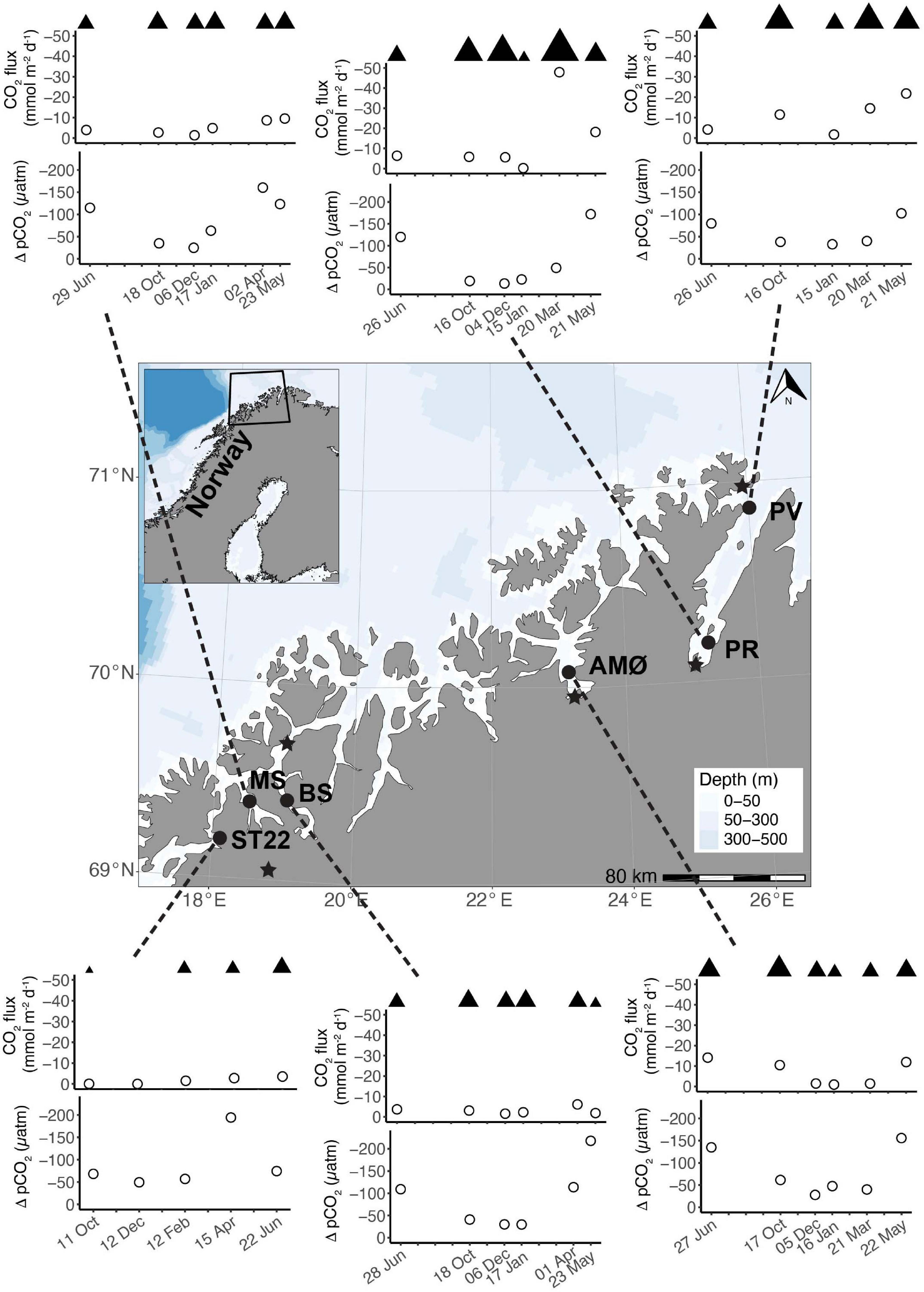
Figure 1. Map of investigated study area along the coast of northern Norway and time series of CO₂ flux (mmol m^–2 d^–1) and ΔpCO₂ (μatm) between June 2018 and 2019. Note different sampling months at ST22. Wind speeds >1 m s^–1 are marked with ▲ above CO₂ flux as relative difference between stations and sampling events. Map: location of stations; PV and PR in Porsangerfjord, AMØ in Altafjord, BS in Balsfjord, MS in Malangen Fjord, and ST22 in Finnfjord Indre. Meteorological stations are indicated with ★.

TABLE 1

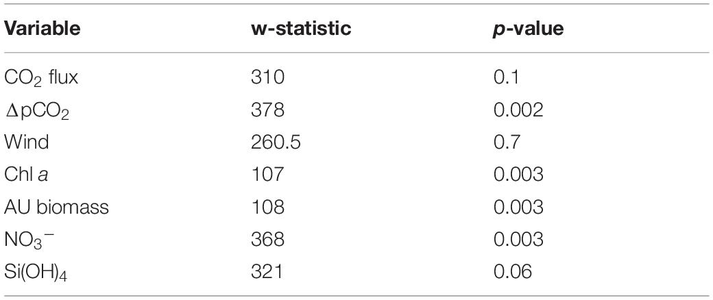
Table 1. Mann-Whitney U test analysis of possible summer (April, May, and June) seasonality in variable of interest: CO₂ flux, ΔpCO₂, wind, chl a, and AU biomass.

Net transport of CO₂ was from the atmosphere to seawater, as represented by negative flux values calculated through the duration of the study (Figure 1). The CO₂ flux did not follow the seasonal variation of surface water ΔpCO₂. That is, the rates sea-air CO₂ flux were not always positively correlated to the greatest sea-air ΔpCO₂. For example, ΔpCO₂ at BS in Balsfjord was twice as high in May than in April, but the instantaneous rate of CO₂ uptake was greater in April. Similar occurrences were observed at all the stations. The summertime variance of CO₂ flux did not statistically differ from that of the annual variance (Mann-Whitney U; w = 310, p = 0.1, Table 1). The two northernmost stations PV and PR in Porsangerfjord (Figure 1), showed the greatest variability and magnitude of CO₂ flux within the time series, ranging from −21.8 ± 1.49 to −1.7 ± 0.27 mmol m^–2 d^–1 and from −47.9 ± 0.35 to −0.2 ± 0.02 mmol m^–2 d^–1, respectively (Figure 1). This observation was in contrast with the seasonal variation observed from stations located in the other three fjords, AMØ (Altafjord), BS (Balsfjord) and MS (Malangen Fjord), which displayed a lower total magnitude and extent of variability of CO₂ flux, with range of −14.1 ± 0.17 to −0.9 ± 0.11 mmol m^–2 d^–1 (Figure 1). Finnfjord Indre (ST22) also maintained net sea-air (i.e., negative) CO₂ flux through the study period (Figure 1). Although the CO₂ flux measured from ST22 showed considerably less variation as compared to the fjord stations, ranging only from −3.6 ± 0.72 to −0.0 ± < 0.00 mmol m^–2 d^–1 across the seasons. In fact, CO₂ flux was nearly constant through the study period, though a slight increase was detected in spring and summer (Figure 1).

Geophysical Environment

The northernmost station PV in the outer part of Porsangerfjord (Figure 1), maintained a largely homogenous water column throughout sample seasons, as compared to other stations. Furthermore, the MLD varied around 100 m, except in June at 30 m (Table 2 and Supplementary Figure 1). At the other fjord stations, the MLD was shallower through summer and autumn <15 m, except 39 m at PR (inner Porsangerfjord) in October (Table 2 and Supplementary Figures 1–5). Stations BS (Balsfjord) and PR (inner Porsangerfjord) had nearly or completely mixed water columns between December and March/April. In contrast, the shallowest MLD occurred through winter measurements, in addition to summer and autumn, at MS in the southernmost fjord Malangen Fjord, and between January and March at AMØ (Altafjord). At ST22 in Finnfjord Indre, the MLD depth varied between 14 and 33 m and showed similar trend in information to BS and PR (Table 2 and Supplementary Figure 6).

TABLE 2

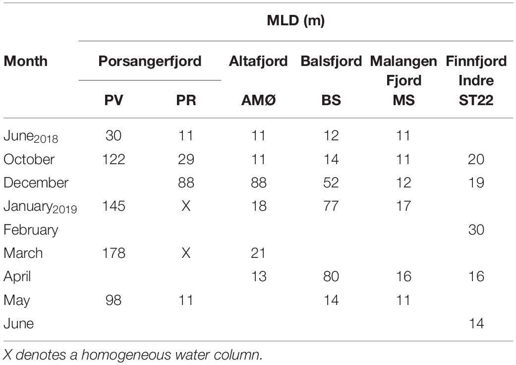
Table 2. Mixed layer depth (MLD) based on density gradient.

The temperature-salinity plot (Figure 2A) shows that BS in Balsfjord and PR in inner Porsangerfjord were in general characterized by lower salinity (<34) than other stations. Also, the temperature range in entire water column at BS was smaller than at other stations, except PV in outer Porsangerfjord (Figure 1 and Table 3). PV in outer Porsangerfjord, AMØ in Altafjord, MS in Malangen Fjord and ST22 in Finnfjord Indre showed more similar salinity range (34–35) in subsurface water corresponding the upper salinity range of Norwegian Coastal Water (<35). The large salinity scatter is mainly from low salinity at uppermost 20–30 m at AMØ in June and at MS in May-June (Figure 2A and Supplementary Figures 3, 5). The lowest subsurface water temperature corresponds at most stations to the lower temperature range of Norwegian Coastal Water (<4°C).

FIGURE 2

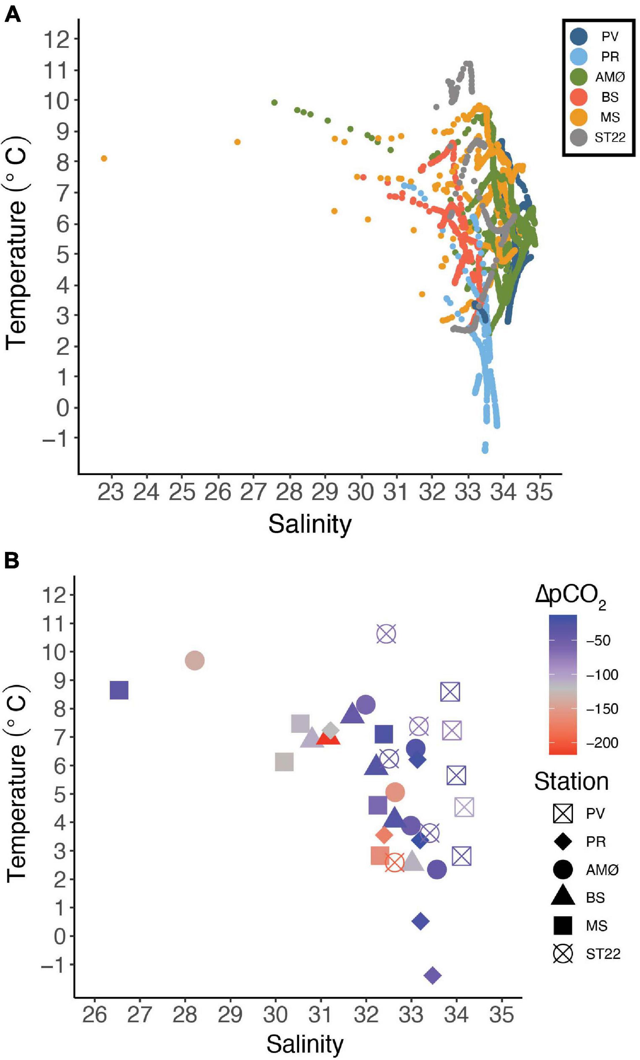
Figure 2. Temperature-salinity (A) plot from June 2018–2019 showing all the CTD casts from stations marked with different colors. (B) Temperature-salinity relationship in surface water (5 m) and ΔpCO₂ (μatm) visualized by colors and stations with different symbols (note the different scales on salinity).

TABLE 3

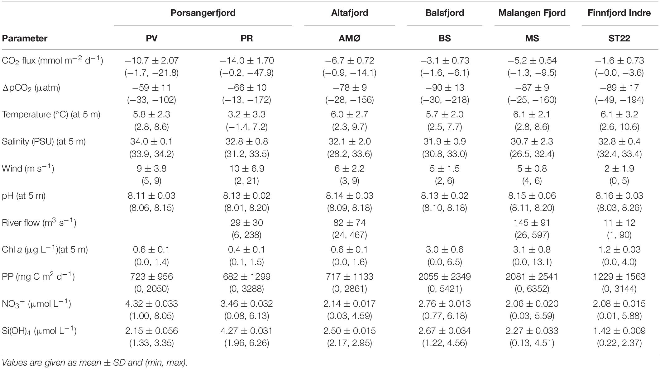
Table 3. Summary of all the measured parameters.

The water temperature at 5 m depth, where CO₂ measurements were collected for all sites, decreased at all the stations from October to March/April, where it reached its lowest measured values in the surface waters, and thereafter increased rapidly (Supplementary Figures 1–6). The surface water temperature varied between 2.3 and 9.7°C at PV, AMØ, BS and MS stations. At PR in inner Porsangerfjord the surface water temperature was lower, −1.4 to 7.2°C, thus the entire water column was close to freezing during winter. In Finnfjord Indre at ST22 the lowest surface water temperature (2.6°C) was similar to PV, AMØ, BS and MS whereas the maximum measured temperature was higher, 10.6°C (Table 3).

The daily average freshwater input by rivers was highest in June 2018 (600 m³ s^–1) and May 2019 (500 m³ s^–1) in the fjords, and in the end of April and May 2019 (45–90 m³ s^–1) in Finnfjord Indre (Supplementary Figure 7). The strongest impact of freshwater input on salinity at 5 m depth (26.5–32.4) was at MS in Malangen Fjord (Table 3), where the Malangen River transported large quantities of meltwater from inland drainages in May and June (max. flow rate 600 m³ s^–1), but also freshwater peaks (flow rate >250 m³ s^–1) occurred in August, December and February (Supplementary Figure 7). The surface water salinity range in Porsangerfjord at PV and PR, and in Balsfjord at BS was between 30.8 and 34.2 (Figure 2B). AMØ in Altafjord also showed pronounced variability between 28.2 and 33.6 (Figure 2B). Finnfjord Indre had the smallest freshwater input (Supplementary Figure 7), and the surface water salinity range at ST22 was relatively small (32.4–33.4; Table 3).

Intermediate winds (4–15 m s^–1) were prevailing at fjord stations, as compared to relatively low winds (<4 m s^–1), except in June (5 m s^–1), recorded at the Finnfjord Indre station (Figure 1 and Supplementary Table 3). Wind speed did not show a seasonal trend (Mann-Whitney U; w = 260.5, p = 0.7, Table 1). Porsangerfjord was subjected to the highest wind speeds (range 2–21 m s^–1) as compared to the other fjords (2–9 m s^–1), except in June and January when difference between all fjord stations was smaller as total range between stations was 2–7 m s^–1 (Figure 1 and Supplementary Table 3). In Finnfjord Indre, wind speed was lower (0.3–5 m s^–1) than in fjords through the study period (Figure 1 and Supplementary Table 3).

Seasonal pH levels observed from ST22 in Finnfjord Indre were different as compared to the respective fjord stations. Specifically, the pH fluctuated to a greater extent and showed two maximum peaks found in October 8.23 ± 0.01 and in April 8.26 ± 0.02. It also showed two minimum peaks observed in February 8.03 ± 0.01 and in June 8.14 ± 0.02 (Supplementary Figure 8). At PR (Porsangerfjord) pH variability was slightly greater (8.01 ± 0.01 to 8.20 ± 0.01) than in the other fjord stations (8.06 ± 0.02 to 8.20 ± 0.02; Table 3). The minimum pH level at stations in Porsangerfjord was measured in March whereas in other fjords it occurred mainly in December-January (Supplementary Figure 8).

The concentration of nitrate (NO₃^–), was found to be strongly seasonal (Mann-Whitney U; w = 368, p < 0.05; Table 1), whereas silicate (Si(OH)₄) showed weaker winter-summer contrast w = 321, p = 0.06; Table 1). Most of stations showed similar seasonal trends for these nutrient concentrations measured from 5 m (Supplementary Figure 9). Concentrations of both nutrients increased from June/October to January/March and thereafter dropped in April/May. These nutrients were depleted in April at the southern stations (BS, MS and ST22) where the range between stations was <1.6 μmol L^–1 NO₃^–, 0.1–1.2 μmol L^–1 Si(OH)₄). Thereafter, the concentration of silicate increased (range between stations 1.3–3.3 μmol L^–1) in May/June, while nitrate concentrations remained nearly constant through summer (Supplementary Figure 9).

Seasonal Phytoplankton Dynamics

Phytoplankton biomass at all sample stations (Figure 3B) varied to a large extent with season, as also supported by the depth-discrete chl a measurements (Figure 3A) and fluorescence profiles (Supplementary Figures 1–5). The highest chl a values were observed in April, 6.6 ± 0.4 and 13.1 ± 0.8 μg L^–1 at 5 m within the southernmost fjord stations BS and MS, respectively (Figure 3A). The northernmost stations (PV, PR and AMØ) maintained relatively low chl a concentration across the measured time series and showed peaks in chl a that ranged between 1.4 ± 0.1 and 3.2 ± 0.3 μg L^–1 in May-June (Figure 3A). ST22 in Finnfjord Indre showed an increase in chl a concentration in April, where the maximum measured chl a at 20 m was 7.5 ± 0.5 μg L^–1 (Figure 3A).

FIGURE 3

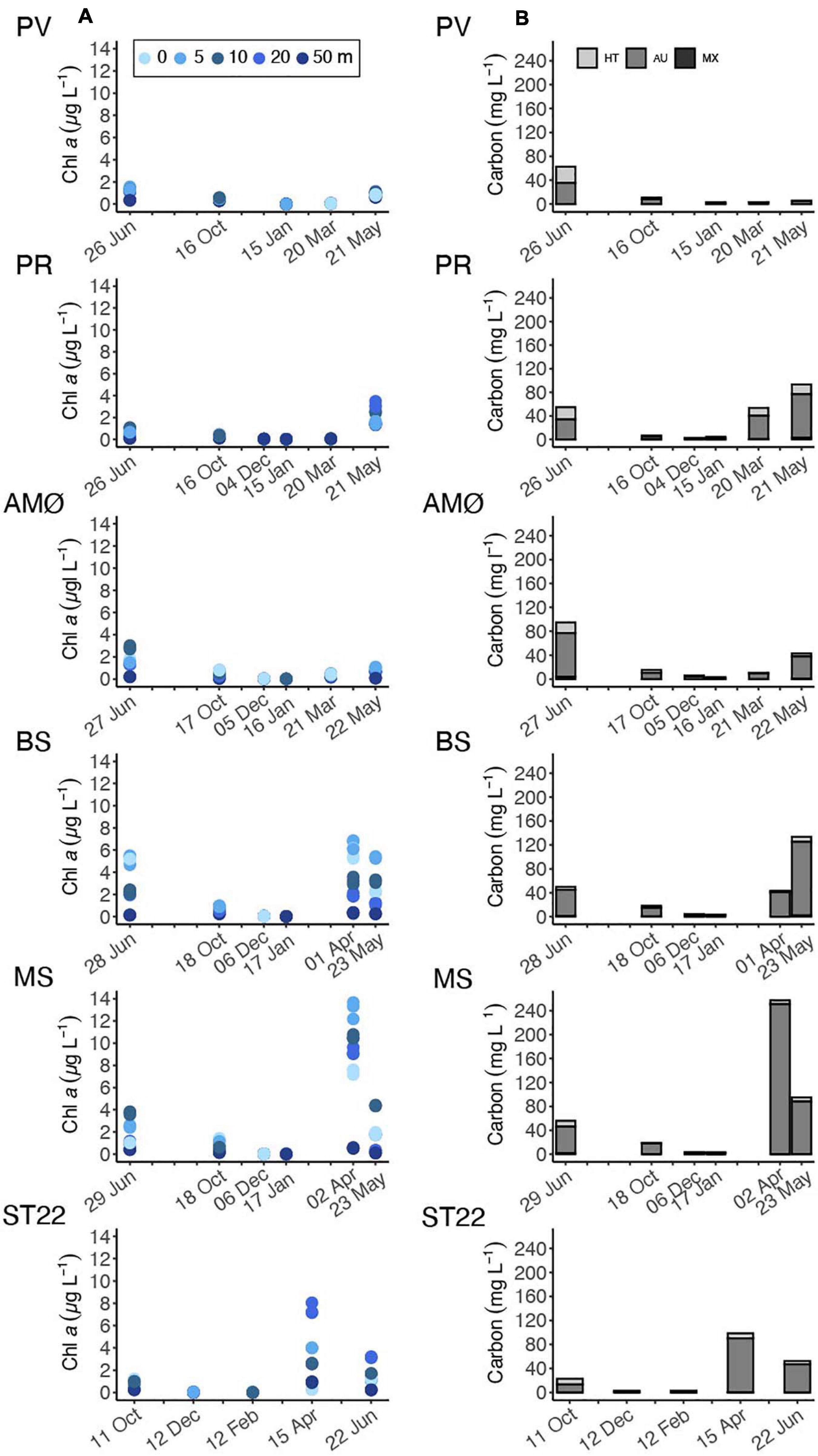
Figure 3. Time series of (A) chl a concentration at discrete sampling depths of 0, 5, 10, 20, and 50 m. (B) Phytoplankton biomass estimated as carbon content from cellular biovolume and cellular carbon content and divided into trophic types: heterotrophic (HT), autotrophic (AU) and, mixotrophic (MX). Note different sampling months at ST22.

During spring and summer, the total phytoplankton biomass (expressed in terms of estimated carbon content), varied between 43 and 257 mg C L^–1 at all stations (Figure 3B). Strong summer seasonality was found on autotrophic phytoplankton biomass (AU biomass) (Mann-Whitney U; w = 108, p < 0.05; Table 1). Peaks of AU biomass blooms varied between April and June among the different fjord stations and was found in April in Finnfjord Indre at ST22 (Figure 3B). At most stations, the biomass of heterotrophic phytoplankton showed a slight increase in summer and autumn. The highest heterotroph/autotroph ratios (∼ 50 %) were observed in Porsangerfjord, where ciliates formed the majority of cells classified as heterotrophic biomass. The fraction of mixotrophic phytoplankton was very small through the study period and the main species was classified as a Mesodinium rubrum.

Estimated daily and maximum net PP showed variation between fjord stations. In April, PP was highest at MS in Malangen Fjord (6352 mg C m^–2 d^–1), whereas at PR in inner Porsangerfjord the highest PP (3288 mg C m^–2 d^–1) occurred in May and at BS in Balsfjord (5421 mg C m^–2 d^–1), AMØ (2861 mg C m^–2 d^–1) and PV in outer Porsangerfjord (2050 mg C m^–2 d^–1) in June (Figure 4 and Table 3). At fjord stations the estimated PP varied most in June, when PV showed lowest 2050 mg C m^–2 d^–1 and BS highest 5421 mg C m^–2 d^–1 value. At ST22, in Finnfjord Indre, the PP was similar between April (3144 mg C m^–2 d^–1) and June (2713 mg C m^–2 d^–1) (Figure 4). In October the PP was slightly higher at ST22 (288 mg C m^–2 d^–1) than at fjord stations. During winter the PP was negligible, i.e., 0 mg C m^–2 d^–1.

FIGURE 4

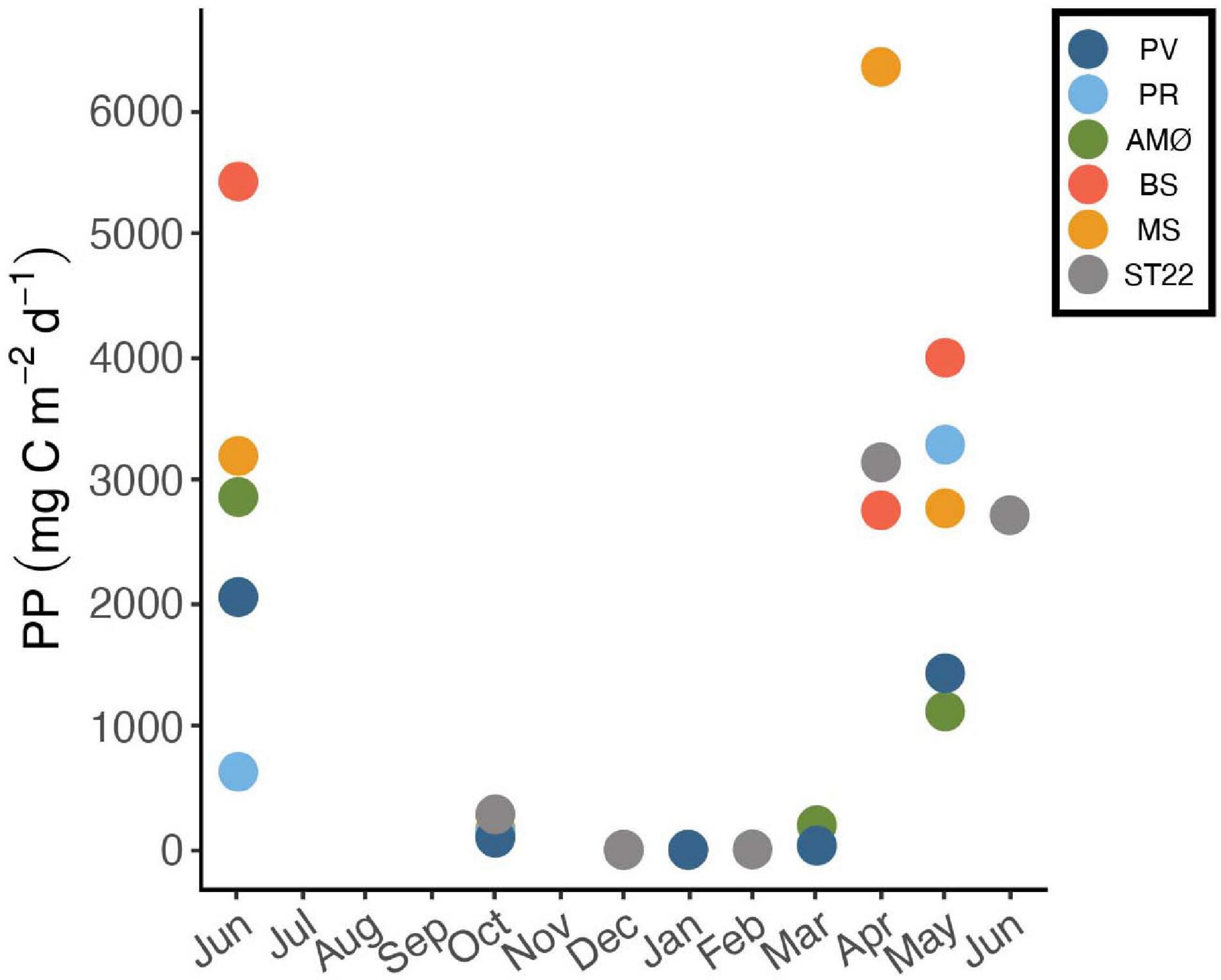
Figure 4. Daily net primary production (PP) of phytoplankton as an average carbon consumption (mg C m^–2 d^–1) in 0–50 m between June 2018 and 2019. Stations are marked with different colors.

Relationship Between ΔpCO₂, CO₂ Flux and Localized Environments

Spearman’s rank correlation on fjord physical-biogeochemical conditions, CO₂ flux and ΔpCO₂ (Figure 5) indicate that surface water pH consistently showed the most frequent and most positive (r = 0.5–0.7; p < 0.05) correlation to ΔpCO₂ across stations and the seasonable time course. Nitrate and silicate concentrations had significant negative correlations with ΔpCO₂ at majority of sampling stations. Also, MLD showed negative correlation (r = −0.8 − –0.5; p < 0.05) at PV, PR and AMØ in the two northernmost fjords (Porsangerfjord and Altafjord) and in Finnfjord Indre at ST22. Biological factors of chl a, total phytoplankton biomass (tot.biomass) and autotrophic phytoplankton biomass (AU biomass) correlated strongly (r = 0.7–1; p < 0.05) with ΔpCO₂ at all stations, except PV where only chl a showed significant positive correlation (Figure 5). Correlation between CO₂ flux and ΔpCO₂ was positive and significant at most of the stations and significant (positive) when evaluated with all data points (r² = 0.16; p = 0.021; Supplementary Figure 10). One or more of the biological factors and wind had positive significant relationship with flux of CO₂ at all the stations except PV, and BS and MS, respectively (Figure 5).

FIGURE 5

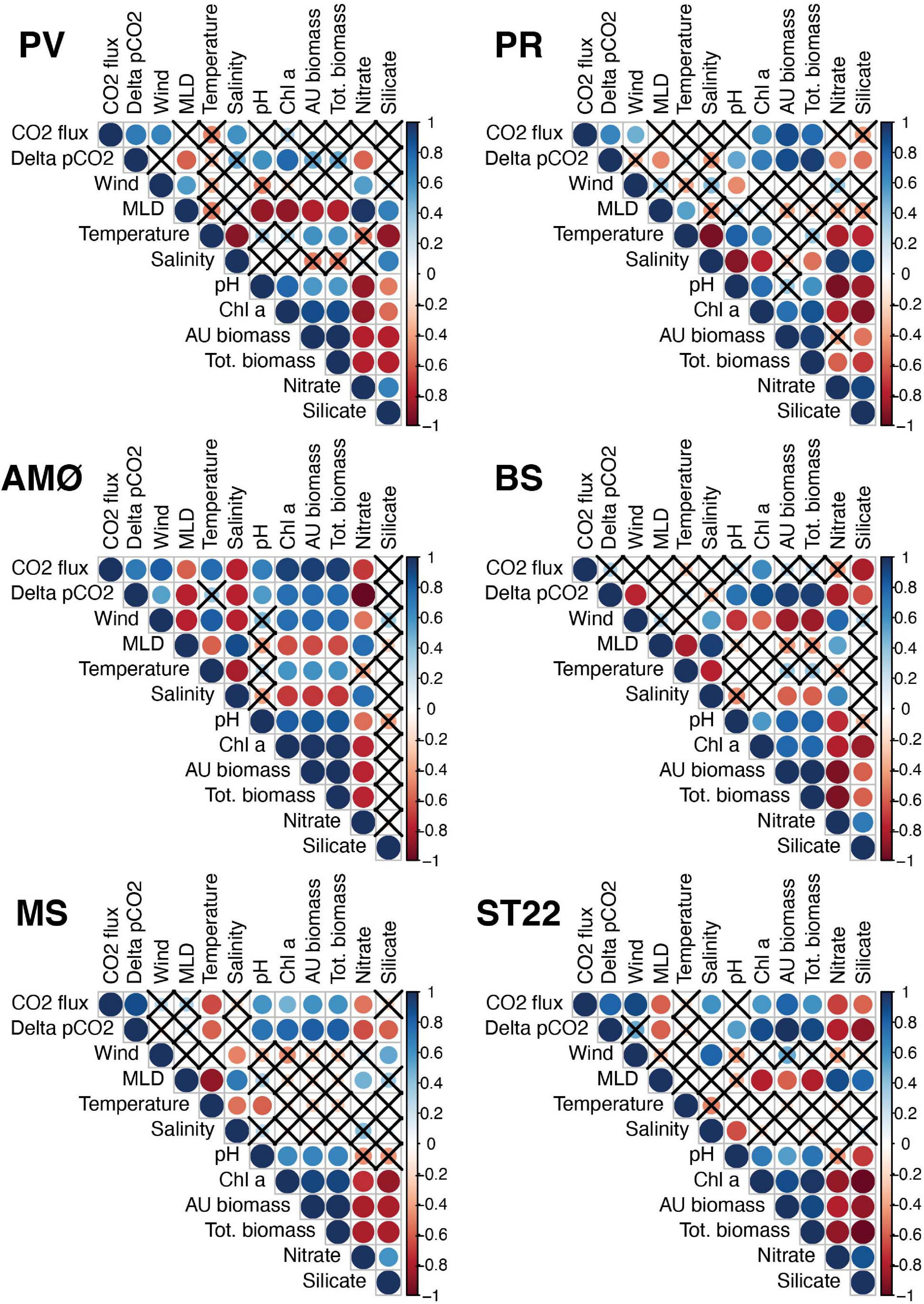
Figure 5. Correlogram of Spearman’s correlation analysis per station. Correlation coefficients between variables are presented in colors and statistical significance is indicated by sizes. Blue color indicates positive and red color negative correlation. Non-significant correlations (p > 0.05) are marked with a cross. Tot. biomass and AU biomass refer to total phytoplankton biomass and autotrophic phytoplankton biomass, respectively.

Redundancy analysis helped reveal that the flux of CO₂ and ΔpCO₂ was not strongly correlated. This is illustrated by nearly perpendicular projections in the RDA triplot (Figure 6). It follows that RDA supports the correlation of physical-biogeochemical properties described above, where high CO₂ flux occurred at strong wind speeds and ΔpCO₂ gradient was strong when primary productivity activity was high. In addition, MLD and temperature have clear negative relationship to ΔpCO₂ and flux of CO₂, respectively. The main difference inferred from correlations between samples at each station is that Finnfjord Indre station (ST22) differ from fjord stations, especially from PV, PR and AMØ with respect to wind speed and strength of CO₂ flux but not with environmental factors contributing to RDA1 and obtained range of variation of ΔpCO₂ within stations. The seasonal pattern of ΔpCO₂ is clearly shown in RDA analysis as it was weaker from October to March compared to months between April and June (Figure 6).

FIGURE 6

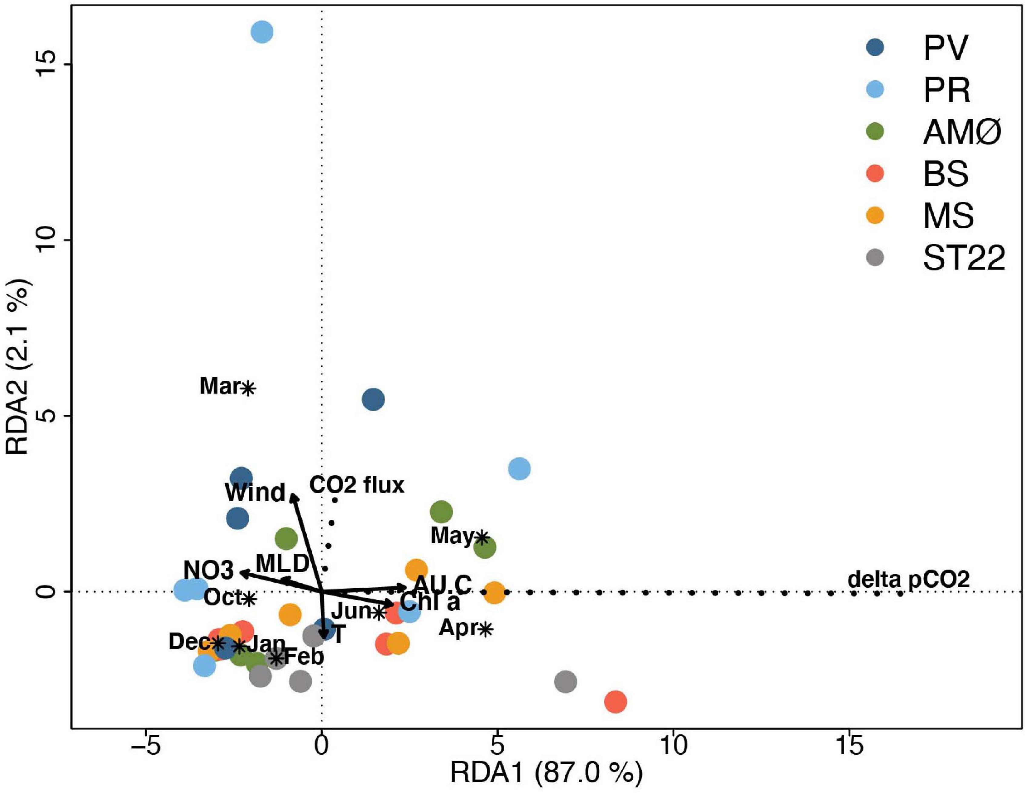
Figure 6. Triplot showing RDA ordination analysis. The eigenvalue of axis 1 (RDA1) and axis 2 (RDA2) are 0.870 and 0.021, respectively, accounting for 89.1% of the total variance. CO₂ flux and ΔpCO₂ represent species (scaled by eigenvalues) and are indicated with dashed lines. Site scores (sampling events) are weighted average of species scores (wa scores) and marked with shapes per station. Quantitative environmental factors are indicated by arrows and qualitative environmental factor (month) by asterix (*) as centroid (weighted average) of site points belonging to the month. The scale marks along the axes apply to qualitative environmental variables and species; quantitative environmental scores were multiplied by 3 to fit in the coordinate system. Stations are marked with different colors.

Discussion

Physical Controls of Seasonality in ΔpCO₂ and CO₂ Flux

Distinct variation in sea-air CO₂ flux between stations was clearly observed despite similar seasonal trends in ΔpCO₂ among stations. Also, the flux of CO₂ did not show the summer-winter seasonality that was prevailing in ΔpCO₂. An expected spring/early summer increase in CO₂ flux was not as clear at all the stations as initially expected, given a low temperature and rapidly increasing CO₂ fixation by predominantly autotrophic phytoplankton. This was especially evident at BS in Balsfjord and ST22 in Finnfjord Indre where increase in CO₂ flux was almost indistinguishable, and in addition, a difference in magnitude was observed between stations during that season (Figure 1). Similar observations of summer-winter contrast between ΔpCO₂ and the flux of CO₂ have been made in Barents Sea where the seasonal variation in CO₂ flux was largely determined by an interaction of wind and ΔpCO₂ (Omar et al., 2007). Turbulence of surface waters as a result of wind velocity are known to have a significant role in controlling the instantaneous rate of sea-air exchange of CO₂ (Wanninkhof, 2014). In this study, the ΔpCO₂ was similar between stations but instantaneous wind speed varied. Therefore, the weak CO₂ uptake in Finnfjord Indre was likely a result of low wind speed and correspondingly, the greatest CO₂ fluxes documented at PR and PV in Porsangerfjord may be attributed to high wind speeds. The total variation in ΔpCO₂ at ST22 in Finnfjord Indre was between −194 and −49 μatm. That was well within the range of ΔpCO₂ values measured at other in-fjord stations, which were between −218 and −13 μatm. As a result, it is unlikely that ΔpCO₂ alone explains the low flux values at this location. Furthermore, modest CO₂ fluxes obtained from Kaldfjord (neighboring our study site in Balsfjord) have been attributed to low wind speed (average 3.3 ± 2.1 m s^–1) (Jones et al., 2020). There, the low wind speed is caused by orographic steering as the fjord is surrounded by steep topography, i.e., mountains, resulting in modest annual carbon uptake compared to for example the Norwegian Sea and the non-ice covered Arctic shelf seas (Jones et al., 2020). At MS in Malangen Fjord, where wind speed was largely constant across seasons (4–6 m s^–1), the variation in CO₂ flux is instead more related to the intensified gradient of CO₂ and changes in surface water temperature (Figures 1, 2B). It follows that the capacity for northern Norwegian fjord systems in this study to act as a CO₂ sink varied considerably with local weather conditions, such as wind. Although, additional high frequency measurements, potentially covering greater spatial resolution are needed to confirm this relationship and to further capture sporadic variability from annual variation.

Given the central role of salinity in driving the surface pCO₂ (Weiss, 1974; Meire et al., 2015; Jones et al., 2020), the significant correlation between surface water salinity and ΔpCO₂ at AMØ in Altafjord is unsurprising. However, riverine inflow in Altafjord was considerably less than in Malangen Fjord (Supplementary Figure 7) where station MS did not show a significant relationship with surface water salinity. The watershed area around Altafjord is the largest among fjords and Finnfjord Indre and therefore it might receive more freshwater runoff and precipitation than implied by the total flow rate of the main rivers. It is possible our correlation analysis did not detect the effect of low salinity on ΔpCO₂ at MS since the surface water salinity at this station was constantly lower (26.5–32.4) than any other station (28.2–34.2). Furthermore, the timing of our sampling in April that recorded the strongest ΔpCO₂ was measured before the pronounced summer and autumn salinity decreases from terrestrial inflow would have occurred (Figure 2B). In comparison, the decreases in salinity in Porsangerfjord, Balsfjord and Finnfjord Indre were briefly present during summer, as seen in CTD-profiles (Supplementary Figures 1, 2, 4, 6). Despite the lack of correlation between salinity and ΔpCO₂ in this study, it is possible that the high ΔpCO₂ in June that occurred after the main spring bloom event can be associated with the surface water freshening as was observed in Kaldfjord where freshwater input in June was related for pronounced decrease in total dissolved inorganic carbon concentration (Jones et al., 2020). This is especially true at PR, AMØ and BS stations that had lower surface water salinities than at PV and ST22 (Figure 2B and Supplementary Figure 7).

The competing effects of warming temperature (warm water holds less CO₂) with PP (autotrophic uptake of CO₂) on ΔpCO₂ was most pronounced at ST22 in Finnfjord Indre in June. This response was also documented at all other stations but to a lesser extent (Figure 1). At ST22 the seasonal increase in temperature from April to June was +4.8°C and there was a simultaneous decrease in ΔpCO₂ of >100 μatm. This is approximately 50 μatm more than the effect of temperature alone, as an increase in water temperature 1°C corresponds ∼10 μatm increase in pCO₂ (Takahashi et al., 1993). Often, the biological fixation of CO₂ compensates the effect of temperature during summer as observed at MS in Malangen Fjord and AMØ in Altafjord (Takahashi et al., 2002; Jones et al., 2020). Therefore, it indicates that at ST22, in addition to temperature and phytoplankton production, other processes affected the ΔpCO₂. The temperature-ΔpCO₂ relationship was only statistically significant at MS, although at all stations high surface water temperature and damped biological activity can be considered to lead to a weakened gradient of pCO₂ in October (Jones et al., 2020). Most likely that can be explained by few data points per station, however, the relationship was not clear in RDA analyses either when all observations were analyzed together.

A weak pycnocline, representing a prolonged period of mixing in the upper water column, has been well documented in northern Norwegian fjords (Reigstad and Wassmann, 1996; Eilertsen and Skarðhamar, 2006). These observations are further supported by this study, where all fjords and Finnfjord Indre bay experienced a weak or an absent pycnocline from late October to March/April (Supplementary Figures 1–6). Deep vertical mixing in winter, together with advection of Norwegian coastal waters, can entrain nutrients and increase salinity in the surface waters of fjords. The inverse relationship between MLD and ΔpCO₂ was statistically significant at PV, PR and AMØ in the two northernmost fjords (Porsangerfjord and Altafjord) and at ST22 in Finnfjord Indre, potentially indicating that the MLD does not drive observed changes in ΔpCO₂ at all fjords sites in this study. Small effects of mixing and advection on pCO₂ (0.1–10 μatm as monthly changes) is also reported in Adventfjorden in Svalbard (Ericson et al., 2018). Although, outcomes from the RDA analysis (Figure 6) suggest that MLD may have a greater influence on ΔpCO₂ during autumn and early winter. Here, the smallest ΔpCO₂ in December can be associated with the timing of water column instability indicating enrichment of CO₂ from subsurface and bottom water similar to observation made in Kaldfjord (Jones et al., 2020). The most pronounced decrease in the strength of ΔpCO₂ occurred at PR in Porsangerfjord suggesting that deepening MLD merges CO₂ enriched subsurface water with higher inorganic carbon content into the surface layer than at other stations. As PR is located behind a shallow sill in the inner part of Porsangerfjord, advection of subsurface water may be partly hindered (Mankettikara, 2013). The lower temperature and salinity (Figure 2A) also indicate that the waters of the inner part of Porsangerfjord (i.e., at PR) are less influenced by Norwegian Coastal Waters than outer Porsangerfjord, Altafjord and Malangen Fjord, where water exchanges with coastal waters including Atlantic Water in summer take place at frequent intervals diminishing the residence time of these fjord waters (Svendsen, 1995; Nordby et al., 1999; Eilertsen and Skarðhamar, 2006). Our measurements of high salinity and temperature below 50 m at PV, AMØ and MS stations support such processes of water mass exchange. Like Porsangerfjord, Balsfjord has low riverine runoff and limited deep water exchange with coastal waters (Svendsen, 1995; Mankettikara, 2013), as supported by generally lower salinity and lower maximum temperature than all other stations, except PV (Figure 2A). Despite the similarity of BS to PR, the ΔpCO₂ in October and December at BS in Balsfjord was not as weak as at PR in inner Porsangerfjord (Figure 1). It is known that fjord circulation in Balsfjord is mainly driven by winds that alternate between down- and up-fjord wind directions (Svendsen, 1995). In spring the change from persistent down-fjord wind (to the fjord opening) to the up-fjord wind leads to the larger inflow of coastal waters into Balsfjord (Svendsen, 1995; Eilertsen and Skarðhamar, 2006). However, the surface waters (upper layer) in Balsfjord might be exchanged relatively frequently with waters from Malangen Fjord, as there is an unique multilayered (separated upper and intermediate layer) circulation (Svendsen, 1995). Shallow Finnfjord Indre with strong current likely transports effectively surface and subsurface water, thus diminishing the effect of mixing observed in autumn and winter on ΔpCO₂ at ST22 compared to fjord stations.

Biological Drawdown of CO₂

Autotrophic phytoplankton consume dissolved CO₂ and thereby reduce pCO₂ in the photic zone. The development of a spring bloom was highly pronounced during sampling of all study locations, with latitude-dependent increases in chl a concentrations increasing over the spring-summer (Figure 3A). Bloom development was first observed in late March of the non-stratified water columns of southernmost fjord stations, BS and MS, as well as the coastal ST22 in Finnfjord Indre. The bloom was subsequently delayed by approximately 1 month in the more northern stations (AMØ, PV and PR) in Altafjord and Porsangerfjord. The strong correlation between ΔpCO₂, biological variables (i.e., chl a and phytoplankton biomass) and nutrient at 5 m supports the strong influence of these phytoplankton blooms on CO₂ drawdown in the fjord systems of this study (Figure 5). The impact of phytoplankton production on ΔpCO₂ was thus most notable from April to June, when average ΔpCO₂ among all the stations was −134 μatm, which is nearly 3.5 times higher than the average taken across autumn and winter months (−40 μatm). The average seasonal ΔpCO₂ amplitude here corresponds to those measured in Kaldfjord in northern Norway and in Godthåbsfjord in Greenland (Meire et al., 2015; Jones et al., 2020). The strong summertime ΔpCO₂ was less extreme at the most open station (PV) where considerably lower chl a and phytoplankton biomass values were measured compared to other stations (Figure 3A). We expect this was a result of the nearly homogenous water column at PV, which occurred as a result of enhanced seawater exchange with the coastal ocean and limited influence freshwater inflow at this location (Supplementary Figures 1, 7). This likely hindered growth of phytoplankton in the surface layer as they are constantly mixed out of the euphotic zone (Eilertsen and Frantzen, 2007).

The estimated net PP per sampling day was high in June and April, especially at BS in Balsfjord and MS in Malangen Fjord (Figure 4), but corresponds to the daily values obtained from 14°C carbon uptake measurements in Balsfjord in April (Eilertsen and Taasen, 1984). The cause of high PP at MS is uncertain. However, it may have been a result of one or a combination of i) high riverine input of nutrients, ii) prominent stratification of the water column facilitating greater light availability through positioning of cells in the upper water column, and iii) greater intensity of downwelling radiation due to the southerly location of this fjord. Between June and July daily net community production of 300–600 mg C d^–1 has been reported in the central Barents Sea, that corresponds to the PP estimated at PV in June (Luchetta et al., 2000). In May, the daily PP estimates at PV and AMØ are in line with, and at BS, PR, MS twice as high as, values obtained in Svalbard (Kongsfjorden) and Greenland (Godthåbsfjord) where highest PP in April/May were 1500–1850 mg C d^–1 (Hodal et al., 2012; Meire et al., 2015). The annual PP was not directly measured here, however, a previous estimate (Eilertsen and Taasen, 1984) of PP (100 g C m^–2 yr^–1) at this latitude indicates that it likely corresponds to or even exceeds at the southernmost stations. The high productivity in northern Norwegian fjords and coastal regions represents a high potential for CO₂ uptake (Smith et al., 2015). In this study, the highest PP was obtained at MS in Malangen Fjord in April corresponding to a CO₂ consumption of 23 g m^–2 d^–1. While an uncertain proportion of the consumed CO₂ will be released back to the atmosphere via respiration, the fate of biologically fixed CO₂ during productive season has an important role determining the saturation state of CO₂ in surface water afterward. If a large part of the produced biomass is exported from the fjords by advection as observed previously in Balsfjord and Malangen Fjord (Reigstad and Wassmann, 1996) then a higher net CO₂ uptake is possible on annual scale.

Flux Estimates in the Context of Existing Knowledge

Our CO₂ flux results correspond, in terms of magnitude, with reported findings from other high-latitude fjords and coastal shelves. The nearest observations are from Kaldfjord (near Balsfjord) with an annual average and maximum CO₂ flux of −0.86 and −2.7 mmol m^–2 d^–1, respectively (Jones et al., 2020). During winter the Norwegian North Atlantic current system is reported to have an average sea-air flux of CO₂ between −6 and −2 mmol m^–2 d^–1 (Olsen et al., 2003) while the annual flux of −11 mmol m^–2 d^–1 was estimated in the Norwegian Sea (Yasunaka et al., 2016). Measurements in sea-ice free Adventfjorden in Svalbard showed sea-air flux to vary between −16 and −4 mmol m^–2 d^–1 across time series of 1 year (Ericson et al., 2018).

It is important to note that the above-mentioned studies applied different methods than were used here. However, with the significant overlap in flux measurements we believe use of the membrane equilibration in nondispersive IR (NDIR) spectrometry-based CO₂ instrument was an effective means of characterizing gradient of CO₂ and exchange of CO₂ gas between the atmosphere and surface water in this study. Furthermore, the parallel study of Jones et al. (2020), whom based their surface water fugacity of CO₂ (pCO₂) determination, and thereafter CO₂ flux calculations, on total inorganic carbon (DIC) and TA values in nearby Kaldfjord with comparable physical (temperature, salinity, wind) and biological conditions, especially Balsfjord and Finnfjord Indre, showed similar magnitudes of CO₂ flux and ΔpCO₂ to what is reported here. Yet, the different methods are not 100 % comparable as it has been shown that depending on choice of the dissociation constants (K1 and K2), computed pCO₂ values from other carbonate system parameters (TA, DIC, pH) can be up to 10 % lower than those of direct measurements (Lueker et al., 2000). Nonetheless, we assume that the estimated annual uptake of atmospheric CO₂ in Kaldfjord was −0.32 ± 0.03 mol C m^–2 can roughly be used as a reference to the Finnfjord Indre and Balsfjord measurements, based on the above-mentioned similarities.

Conclusion

This study was designed to characterize sea-air CO₂ flux along coastal northern Norway in the context of physical and biological factors. From our assessment we find that wind speed is the physical factor which has the greatest effect on the variability in CO₂ flux between stations, followed by the magnitude of atmospheric CO₂ flux. Despite this critical influence of wind speed on flux magnitude, ΔpCO₂ is the main driving force to pull CO₂ gas from atmosphere to sea. The spring-summer phytoplankton bloom has been documented here as a main controlling factor of ΔpCO₂ during the polar day. However, in this study we found that the strong summertime drawdown of CO₂ cannot account for the maintained state of CO₂ undersaturation, with respect to atmosphere, that was documented throughout the year at our study locations. This study provides new spatial and seasonal insights about the strength of carbon sink and CO₂ saturation state in northern Norwegian fjords and coastal regions. Also, this study supports previous estimates that high-latitude coastal areas are undersaturated with respect to atmospheric CO₂. However, better spatial, and temporal coverage within the fjords – scaling from the proximity of freshwater discharge at the head to coastal water inflow at the mouth of the fjord – is needed to further characterize the complex trends of sea-air CO₂ flux in these systems, and to quantify the annual CO₂ uptake representing the entire region. With a warmer future climate, the strong seasonality in freshwater input is expected to change and as a result longer stratification period becomes likely prevailing in this region that can influence mixing of the water column and phytoplankton bloom dynamics and thus potential change in atmospheric carbon uptake is possible. To further understand how such changing freshwater inputs will affect the hydrography and water circulation with related CO₂ flux in these fjords, more detailed studies of water mass exchange and circulation, including the role of advection, should be included in future studies.

Data Availability Statement

The original contributions presented in the study are included in the article/Supplementary Material, further inquiries can be directed to the corresponding author. All data, calculations and figure generation scripts are provided and linked to R markdown files deposited on the Open Science Framework project: Northern Norwegian Fjord CO2 Flux (https://osf.io/tbzse/).

Author Contributions

NJA, HCB, and HCE conceptualized the study. NJA conducted the field work, sample processing, the main analysis, and wrote the manuscript draft. HCE provided the primary production estimates. KC helped with nutrient analyses. All authors contributed to the final version.

Funding

This study was supported by strategic funds from UiT – The Arctic University of Norway allocated to understanding environmental impacts of the project Mass Cultivation of Diatoms at Finnfjord AS and was also supported by contributions from ARC- The Arctic Centre for Sustainable Energy. Work by KC was supported by the Diatom ARCTIC project (NE/R012849/1; 03F0810A), part of the Changing Arctic Ocean program, jointly funded by the UKRI Natural Environmental Research Council (NERC) and the German Federal Ministry of Education and Research (BMBF).

Conflict of Interest

The authors declare that the research was conducted in the absence of any commercial or financial relationships that could be construed as a potential conflict of interest.

Acknowledgments

We would gratefully thank the captain and crew of RV Johan Ruud for the fieldwork support. We acknowledge Ingeborg Giæver (UiT) and Reetta Sætre for the help on fieldwork in Finnfjord Indre as well as the collaborations between Finnfjord AS and UiT-The Arctic University of Norway that support field sampling facilities.

Supplementary Material

The Supplementary Material for this article can be found online at: https://www.frontiersin.org/articles/10.3389/fmars.2021.692093/full#supplementary-material

Footnote

1. ^ https://osf.io/tbzse/

References

Bates, N. R. (2006). Air-sea CO2fluxes and the continental shelf pump of carbon in the Chukchi Sea adjacent to the Arctic Ocean. J. Geophys. Res. 111:C10013. doi: 10.1029/2005jc003083

CrossRef Full Text | Google Scholar

Bax, N., and Eliassen, J.-E. (1990). Multispecies analysis in Balsfjord, northern Norway: solution and sensitivity analysis of a simple ecosystem model. ICES J. Mar. Sci. 47, 175–204. doi: 10.1093/icesjms/47.2.175

CrossRef Full Text | Google Scholar

Chen, C. T. A., Huang, T. H., Chen, Y. C., Bai, Y., He, X., and Kang, Y. (2013). Air–sea exchanges of CO2 in the world’s coastal seas. Biogeosciences 10, 6509–6544. doi: 10.5194/bg-10-6509-2013

CrossRef Full Text | Google Scholar

Degerlund, M., and Eilertsen, H. C. (2010). Main species characteristics of phytoplankton spring blooms in NE Atlantic and Arctic waters (68–80 N). Estuaries Coasts 33, 242–269. doi: 10.1007/s12237-009-9167-7

CrossRef Full Text | Google Scholar

Delaigue, L., Helmuth, T., and Mucci, A. (2020). Spatial variations in CO 2 fluxes in the Saguenay Fjord (Quebec, Canada) and results of a water mixing model. Biogeosciences 17, 547–566. doi: 10.5194/bg-17-547-2020

CrossRef Full Text | Google Scholar

Edler, L., and Elbrächter, M. (2010). “The utermöhl method for quantitative phytoplankton analysis,” in Microscopic and Molecular Methods for Quantitative Phytoplankton Analysis, Vol. 110, eds B. Karlson, C. Cusack, and E. Bresnan (Paris: Intergovernmental Oceanographic Commission Manual and guides), 13–20.

Google Scholar

Eilertsen, H. C., and Degerlund, M. (2010). Phytoplankton and light during the northern high-latitude winter. J. Plankton Res. 32, 899–912. doi: 10.1093/plankt/fbq017

PubMed Abstract | CrossRef Full Text | Google Scholar

Eilertsen, H. C., and Frantzen, S. (2007). Phytoplankton from two sub-Arctic fjords in northern Norway 2002–2004: I. Seasonal variations in chlorophyll a and bloom dynamics. Mar. Biol. Res. 3, 319–332. doi: 10.1080/17451000701632877

CrossRef Full Text | Google Scholar

Eilertsen, H. C., and Holm-Hansen, O. (2000). Effects of high latitude UV radiation on phytoplankton and nekton modelled from field measurements by simple algorithms. Polar Res. 19, 173–182. doi: 10.3402/polar.v19i2.6543

CrossRef Full Text | Google Scholar

Eilertsen, H. C., and Skarðhamar, J. (2006). Temperatures of north Norwegian fjords and coastal waters: variability, significance of local processes and air–sea heat exchange. Estuar. Coast. Shelf Sci. 67, 530–538. doi: 10.1016/j.ecss.2005.12.006

CrossRef Full Text | Google Scholar

Eilertsen, H. C., and Taasen, J. (1984). Investigations on the plankton community of Balsfjorden, northern Norway. The phytoplankton 1976–1978. Environmental factors, dynamics of growth, and primary production. Sarsia 69, 1–15. doi: 10.1080/00364827.1984.10420584

CrossRef Full Text | Google Scholar

Ericson, Y., Falck, E., Chierici, M., Fransson, A., and Kristiansen, S. (2019). Marine CO2 system variability in a high arctic tidewater-glacier fjord system, Tempelfjorden, Svalbard. Cont. Shelf Res. 181, 1–13. doi: 10.1016/j.csr.2019.04.013

CrossRef Full Text | Google Scholar

Ericson, Y., Falck, E., Chierici, M., Fransson, A., Kristiansen, S., Platt, S. M., et al. (2018). Temporal variability in surface water pCO2 in Adventfjorden (West Spitsbergen) with emphasis on physical and biogeochemical drivers. J. Geophys. Res. Oceans 123, 4888–4905. doi: 10.1029/2018jc014073

CrossRef Full Text | Google Scholar

Frouin, R., Lingner, D. W., Gautier, C., Baker, K. S., and Smith, R. C. (1989). A simple analytical formula to compute clear sky total and photosynthetically available solar irradiance at the ocean surface. J. Geophys. Res. Oceans 94, 9731–9742. doi: 10.1029/jc094ic07p09731

CrossRef Full Text | Google Scholar

Hansen, G. A., and Eilertsen, H. C. (1995). “Modelling the onset of phytoplankton blooms: a new approach,” in Ecology of Fjords and Coastal Waters, eds H. R. Skjoldal, C. Hopkins, K. E. Erikstad, and H. P. Leinaas (Amsterdam: Elsevier Science).

Google Scholar

Hartman, B., and Hammond, D. E. (1985). “Gas exchange in San Francisco Bay,” in Temporal Dynamics of an Estuary: San Francisco Bay. Developments in Hydrobiology, eds J. E. Cloern and F. H. Nichols (Dordrecht: Springer), 59–68. doi: 10.1007/978-94-009-5528-8_4

CrossRef Full Text | Google Scholar

Hodal, H., Falk-Petersen, S., Hop, H., Kristiansen, S., and Reigstad, M. (2012). Spring bloom dynamics in Kongsfjorden, Svalbard: nutrients, phytoplankton, protozoans and primary production. Polar Biol. 35, 191–203. doi: 10.1007/s00300-011-1053-7

CrossRef Full Text | Google Scholar

Holm-Hansen, O., and Riemann, B. (1978). Chlorophyll a determination: improvements in methodology. Oikos 30, 438–447. doi: 10.2307/3543338

CrossRef Full Text | Google Scholar

Iqbal, M. (2012). An Introduction to Solar Radiation. Amsterdam: Elsevier.

Google Scholar

Jones, E. M., Renner, A. H., Chierici, M., Wiedmann, I., Lødemel, H. H., and Biuw, M. (2020). Seasonal dynamics of carbonate chemistry, nutrients and CO 2 uptake in a sub-Arctic fjord. Elem. Sci. Anth. 8:41.

Google Scholar

Larsen, L.-H. (2015). Program for Miljøundersøkelse i Vannforekomsten Finnfjorden Indre i Lenvik kommune, Troms Fylke. Tromsø: Akvaplan-niva.

Google Scholar

Luchetta, A., Lipizer, M., and Socal, G. (2000). Temporal evolution of primary production in the central Barents Sea. J. Mar. Syst. 27, 177–193. doi: 10.1016/s0924-7963(00)00066-x

CrossRef Full Text | Google Scholar

Lueker, T. J., Dickson, A. G., and Keeling, C. D. (2000). Ocean pCO2 calculated from dissolved inorganic carbon, alkalinity, and equations for K1 and K2: validation based on laboratory measurements of CO2 in gas and seawater at equilibrium. Mar. Chem. 70, 105–119. doi: 10.1016/s0304-4203(00)00022-0

CrossRef Full Text | Google Scholar

Mankettikara, R. (2013). Hydrophysical Characteristics of the Northern Norwegian Coast and Fjords. Doctoral, Thesis. Tromsø: University of Tromsø.

Google Scholar

Meire, L., Søgaard, D., Mortensen, J., Meysman, F., Soetaert, K., Arendt, K., et al. (2015). Glacial meltwater and primary production are drivers of strong CO2 uptake in fjord and coastal waters adjacent to the Greenland Ice Sheet. Biogeosciences 12, 2347–2363. doi: 10.5194/bg-12-2347-2015

CrossRef Full Text | Google Scholar

Michelsen, H. K., Svensen, C., Reigstad, M., Nilssen, E. M., and Pedersen, T. (2017). Seasonal dynamics of meroplankton in a high-latitude fjord. J. Mar. Syst. 168, 17–30. doi: 10.1016/j.jmarsys.2016.12.001

CrossRef Full Text | Google Scholar

Nordby, E., Tande, K. S., Svendsen, H., Slagstad, D., and Båmstedt, U. (1999). Oceanography and fluorescence at the shelf break off the north Norwegian coast (69°’ N-70° 30’ N) during the main productive period in 1994. Sarsia 84, 175–189. doi: 10.1080/00364827.1999.10420424

CrossRef Full Text | Google Scholar

Norwegian Environment Agency (2021). Finnfjord – Releases of Carbon Dioxide fossil (CO2 (F)). Available online at: https://www.norskeutslipp.no/en/Miscellaneous/Company/?CompanyID=5712&ComponentPageID=180 (accessed February 03, 2021)

Google Scholar

Oksanen, J., Blanchet, F. G., Kindt, R., Legendre, P., Minchin, P., O’hara, R., et al. (2013). Community Ecology Package. R Package Version 2(0).

Google Scholar

Olsen, A., Bellerby, R. G., Johannessen, T., Omar, A. M., and Skjelvan, I. (2003). Interannual variability in the wintertime air–sea flux of carbon dioxide in the northern North Atlantic, 1981–2001. Deep Sea Res. Part I Oceanogr. Res. Pap. 50, 1323–1338. doi: 10.1016/s0967-0637(03)00144-4

CrossRef Full Text | Google Scholar

Omar, A. M., Johannessen, T., Olsen, A., Kaltin, S., and Rey, F. (2007). Seasonal and interannual variability of the air–sea CO2 flux in the Atlantic sector of the Barents Sea. Mar. Chem. 104, 203–213. doi: 10.1016/j.marchem.2006.11.002

CrossRef Full Text | Google Scholar

Oug, E., and Høisœter, T. (2000). Soft-bottom macrofauna in the high-latitude ecosystem of Balsfjord, northern Norway: species composition, community structure and temporal variability. Sarsia 85, 1–13. doi: 10.1080/00364827.2000.10414551

CrossRef Full Text | Google Scholar

Peralta-Ferriz, C., and Woodgate, R. A. (2015). Seasonal and interannual variability of pan-Arctic surface mixed layer properties from 1979 to 2012 from hydrographic data, and the dominance of stratification for multiyear mixed layer depth shoaling. Prog. Oceanogr. 134, 19–53. doi: 10.1016/j.pocean.2014.12.005

CrossRef Full Text | Google Scholar

R Core Team (2013). R: A Language and Environment for Statistical Computing. Vienna: R Foundation for Statistical Computing.

Google Scholar

Reigstad, M., and Wassmann, P. (1996). Importance of advection for pelagic-benthic coupling in north Norwegian fjords. Sarsia 80, 245–257. doi: 10.1080/00364827.1996.10413599

CrossRef Full Text | Google Scholar

Rysgaard, S., Mortensen, J., Juul-Pedersen, T., Sørensen, L. L., Lennert, K., Søgaard, D., et al. (2012). High air–sea CO2 uptake rates in nearshore and shelf areas of Southern Greenland: temporal and spatial variability. Mar. Chem. 128, 26–33. doi: 10.1016/j.marchem.2011.11.002

CrossRef Full Text | Google Scholar

Sejr, M., Krause-Jensen, D., Rysgaard, S., Sørensen, L., Christensen, P., and Glud, R. N. (2011). Air—sea flux of CO2 in arctic coastal waters influenced by glacial melt water and sea ice. Tellus B Chem. Phys. Meteorol. 63, 815–822. doi: 10.1111/j.1600-0889.2011.00540.x

CrossRef Full Text | Google Scholar

Skarðhamar, J., and Svendsen, H. (2005). Circulation and shelf–ocean interaction off North Norway. Cont. Shelf Res. 25, 1541–1560. doi: 10.1016/j.csr.2005.04.007

CrossRef Full Text | Google Scholar

Smith, R. W., Bianchi, T. S., Allison, M., Savage, C., and Galy, V. (2015). High rates of organic carbon burial in fjord sediments globally. Nat. Geosci. 8, 450–453. doi: 10.1038/ngeo2421

CrossRef Full Text | Google Scholar

Strickland, J. D. H., and Parsons, T. R. (1972). “Determination of carbonate, bicarbonate, and free carbon dioxide from pH and alkalinity measurements,” in A Practical Hand Book of Seawater Analysis, 2nd Edn, ed. J. C. Stevenson (Ottawa, ON: Fisheries Research Board of Canada), 310.

Google Scholar

Svendsen, H. (1995). “Physical oceanography of coupled fjord-coast systems in northern Norway with special focus on frontal dynamics and tides,” in Ecology of Fjords and Coastal Waters, eds H. R. Skjoldal, C. Hopkins, K. E. Erikstad, and H. P. Leinaas (Amsterdam: Elsevier), 149–164.

Google Scholar

Takahashi, T., Olsson, J., Goddard, J. G., Chipman, D. W., and Sutherland, S. (1993). Seasonal variation of CO2 and nutrients in the high-latitude surface oceans: a comparative study. Global Biogeochem. Cycles 7, 843–878. doi: 10.1029/93gb02263

CrossRef Full Text | Google Scholar

Takahashi, T., Sutherland, S. C., Sweeney, C., Poisson, A., Metzl, N., Tilbrook, B., et al. (2002). Global sea-air CO2 flux based on climatological surface ocean PCO2 and seasonal biological and temperature effects. Deep Sea Res. Part II Top. Stud. Oceanogr. 49, 1601–1622. doi: 10.1016/s0967-0645(02)00003-6

CrossRef Full Text | Google Scholar

Telmer, K., and Veizer, J. (1999). Carbon fluxes, pCO2 and substrate weathering in a large northern river basin, Canada: carbon isotope perspectives. Chem. Geol. 159, 61–86. doi: 10.1016/s0009-2541(99)00034-0

CrossRef Full Text | Google Scholar

Thomas, H., Bozec, Y., Elkalay, K., and De Baar, H. J. (2004). Enhanced open ocean storage of CO2 from shelf sea pumping. Science 304, 1005–1008. doi: 10.1126/science.1095491

PubMed Abstract | CrossRef Full Text | Google Scholar

Tomas, C. R. (1997). Identifying Marine Phytoplankton. Amsterdam: Elsevier.

Google Scholar

Tsunogai, S., Watanabe, S., and Sato, T. (1999). Is there a “continental shelf pump” for the absorption of atmospheric CO2? Tellus B Chem. Phys. Meteorol. 51, 701–712. doi: 10.3402/tellusb.v51i3.16468

CrossRef Full Text | Google Scholar

Wanninkhof, R. (2014). Relationship between wind speed and gas exchange over the ocean revisited. Limnol. Oceanogr. Methods 12, 351–362. doi: 10.4319/lom.2014.12.351

CrossRef Full Text | Google Scholar

Wassmann, P., Svendsen, H., Keck, A., and Reigstad, M. (1996). Selected aspects of the physical oceanography and particle fluxes in fjords of northern Norway. J. Mar. Syst. 8, 53–71. doi: 10.1016/0924-7963(95)00037-2

CrossRef Full Text | Google Scholar

Webb, W. L., Newton, M., and Starr, D. (1974). Carbon dioxide exchange of Alnus rubra. Oecologia 17, 281–291. doi: 10.1007/bf00345747

PubMed Abstract | CrossRef Full Text | Google Scholar

Weiss, R. F. (1974). Carbon dioxide in water and seawater: the solubility of a non-ideal gas. Mar. Chem. 2, 203–215. doi: 10.1016/0304-4203(74)90015-2

CrossRef Full Text | Google Scholar

Włodarska-Kowalczuk, M., Mazurkiewicz, M., Górska, B., Michel, L. N., Jankowska, E., and Zaborska, A. (2019). Organic carbon origin, benthic faunal consumption, and burial in sediments of Northern Atlantic and Arctic Fjords (60–81° N). J. Geophy. Res. Biogeosci. 124, 3737–3751. doi: 10.1029/2019jg005140

CrossRef Full Text | Google Scholar

Yasunaka, S., Murata, A., Watanabe, E., Chierici, M., Fransson, A., van Heuven, S., et al. (2016). Mapping of the air–sea CO2 flux in the Arctic Ocean and its adjacent seas: basin-wide distribution and seasonal to interannual variability. Polar Sci. 10, 323–334. doi: 10.1016/j.polar.2016.03.006

CrossRef Full Text | Google Scholar