
94% of researchers rate our articles as excellent or good
Learn more about the work of our research integrity team to safeguard the quality of each article we publish.
Find out more
ORIGINAL RESEARCH article
Front. Mar. Sci., 26 August 2021
Sec. Ocean Observation
Volume 8 - 2021 | https://doi.org/10.3389/fmars.2021.687414
 Babette C. Tchonang1*
 Mounir Benkiran1
 Pierre-Yves Le Traon1,2
 Simon Jan van Gennip1
 Jean Michel Lellouche1
 Giovanni Ruggiero1
A first attempt was made to quantify the impact of the assimilation of Surface Water Ocean Topography (SWOT) swath altimeter data in a global 1/12° high resolution analysis and forecasting system through a series of Observing System Simulation Experiments (OSSEs). The OSSE framework (Nature Run and Free Run) and data assimilation scheme have been described in detail in a companion article (Benkiran et al., 2021). The impact of assimilating data from SWOT and three nadir altimeters was quantified by estimating analysis and forecast error variances for sea surface height (SSH), temperature, salinity, zonal, and meridional velocities. Wave-number spectra and coherence analyses of SSH errors were also computed. SWOT data will significantly improve the quality of ocean analyses and forecasts. Adding SWOT observations to those of three nadir altimeters globally reduces the variance of SSH and surface velocities in analyses and forecasts by about 30 and 20%, respectively. Improvements are greater in high-latitude regions where space/time coverage of SWOT is much denser. The combination of SWOT data with data from three nadir altimeters provides a better resolution of wavelengths between 50 and 200 km with a more than 40% improvement outside tropical regions with respect to data from three nadir altimeters alone. The study has also highlighted that the impact of using SWOT data is likely to be very different depending on geographical areas. Constraining smaller spatial scales (wavelengths below 100 km) remains challenging as they are also associated with small time scales. Although this is only a first step, the study has demonstrated that SWOT data could be readily assimilated in a global high-resolution analysis and forecasting system with a positive impact at all latitudes and outstanding performances.
Sea surface height (SSH) altimeter measurements are essential for ocean prediction. For nearly three decades, the TOPEX/Poseidon, Jason 1/2 and 3 reference altimeter missions, complemented by missions such as ERS-1/2, ENVISAT, Alti-Ka, Cryosat-2, and Sentinel-3A&B, have been providing SSH measurements that have been used to constrain ocean models through data assimilation (see Le Traon et al., 2017 for a review). While nadir altimeters provide good along-track mesoscale resolution and can detect structures with wavelengths longer than about 50 km (Dufau et al., 2016), the main limitation is the 2D resolution related to the distance between tracks. The combination of several nadir altimeters allows a significant improvement in the representation of the mesoscale in ocean analysis and forecasting systems (e.g., Le Traon et al., 2017; Hamon et al., 2019). At least four altimeters are needed (e.g., Le Traon et al., 2017) but only wavelengths longer than 200 km are well represented.
The representation of the ocean at mesoscale and sub-mesoscale, which is important for understanding ocean dynamics and energy transfer processes in the ocean (e.g., Klein et al., 2019), the coupling between physics and biogeochemistry and for a wide range of ocean applications (e.g., Le Traon et al., 2019), is thus limited by the spatial resolution of nadir altimeters. The future Surface Water Ocean Topography (SWOT) mission developed jointly by NASA (National Aeronautics and Space Administration) and CNES (the French Space Agency) and with a contribution from the United Kingdom and Canadian space agencies (Fu et al., 2009; Morrow et al., 2019) addresses these limitations. The SWOT satellite, to be launched in 2022, will be the first wide-swath altimeter mission. Thanks to a Ka-band radar interferometer (KaRIn), it will extend the capability of existing altimeters to 2D SSH mapping with an unprecedented spatial resolution of up to a 20 km wavelength over a swath width of about 120 km. SWOT will have a repeat cycle of 21 days and the revisit time will vary from about 10 days at the equator to a few days at the high-latitudes. The 21-day SWOT repetition period will not be sufficient to capture the temporal evolution of “small” mesoscale and sub-mesoscale structures (e.g., Ubelmann et al., 2015). Therefore, a major challenge will be to dynamically interpolate SWOT observations and conventional altimeter data in very high-resolution models.
The impact of the future SWOT mission for ocean analysis and forecasting can be analyzed via Observing System Simulation Experiments (OSSEs) (Halliwell et al., 2014). OSSEs are based on two different models. The first model realistically represents the ocean and its spatiotemporal variability. This model is generally referred to as Nature Run (NR) and is used to sample synthetic observations to mimic either an existing or a future observation system. The second model is generally called Assimilated Run (AR) and is used to assimilate synthetic observations computed from NR. The AR performance is evaluated through the comparison with the NR which enables us to quantify the impact of the observations. OSSEs also test the ability of data assimilation systems to efficiently merge different types of observations with models to produce improved ocean analyses and forecasts.
A few first wide-swath altimetry OSSEs have been performed at regional scales (Bonaduce et al., 2018; D’Addezio et al., 2019; Souopgui et al., 2020). They demonstrate the potential impact of SWOT data and the challenge to constrain the smaller wavelengths (typically below 150 km). For the first time, this study proposes global OSSEs with a state-of-the-art and high resolution (1/12°) modeling and data assimilation system. The objective is to assess the potential of SWOT data for global ocean analysis and forecasting and prepare for the ingestion of SWOT data in the Mercator Ocean (MO) global analysis and forecasting system, which is used operationally for the European Copernicus Marine Service and its applications (Le Traon et al., 2019).
For this study, the MO data assimilation system used operationally for a current real-time forecasting system (Lellouche et al., 2018), had to be modified. The main updates of the assimilation scheme, the choice of NR (including its validation) and AR, as well as the design and calibration of the OSSEs have been described in detail in a companion article (Benkiran et al., 2021). In the present article, results from these experiments are analyzed to evaluate the impact of SWOT data assimilation on several parameters: SSH, temperature, salinity, and horizontal velocity fields. Spectral and coherence analyses were carried out to better characterize the SSH spatial scales that can be resolved with SWOT observations. More elaborated Lagrangian diagnostics were also used to assess how SWOT can improve key operational oceanography applications (e.g., the drifting of pollutants).
The article is structured as follows. Following the first introductory section, section “OSSE Experiment” first summarizes the OSSE design and the list of OSSEs that have been carried out. Section “OSSEs Results” analyses the impact of assimilating data respectively from three nadir altimeters, SWOT alone, and SWOT plus three nadir altimeters by evaluating the errors in OSSEs and wavenumber spectra of errors. Lagrangian diagnostics are detailed in section “Lagrangian Diagnostics.” The synthesis, main conclusion and perspectives are given in section “Synthesis, Conclusion, and Perspectives”
The performed ARs are based on the MO assimilation system (SAM – Système d’Assimilation Mercator) and NEMO3.1 model (Madec and The Nemo Team, 2008), like the current global high-resolution MO forecasting system (Lellouche et al., 2018). SAM implements a reduced-order local Kalman Filter for which the analysis subspace is constructed using a band-passed time series of model states from a climatological run. In part 1 of this article (Benkiran et al., 2021), the parameters of the bandpass filtering were revisited to improve the representation of mesoscale (100–400 km) signals. The new set of anomalies has a flatter spectrum that is more coherent with the forecast errors. Reported improvements in error variance are of the order of 15% for the spectral band corresponding to 150–250 km wavelength compared to a twin experiment using the current operational set of anomalies.
Another important aspect is the use of a four-dimensional (4D) version of the filter, i.e., the analysis uses a 4D subspace and produces daily increments (model corrections) of SSH, temperature and salinity (T/S), and zonal and meridional velocities (U/V). The 4D aspect improved the temporal and spatial representation of the forecast error (Benkiran et al., 2021). This fact is most significant for periods shorter than 20 days and longer than 7 days. Therefore, we understand that the time correlation represented in the 4D anomalies is reliable and can be used to fill the gap left by the long repetitiveness time of SWOT orbit in a 7-day window.
The increments are used to force the model equations using the so-called Incremental Analysis Update (IAU; Bloom et al., 1996). We used a 4D version of this method in which the daily increments are interpolated in time and weighted by the inverse of the number of time steps in the assimilation window (Lei and Whitaker, 2016). Therefore, one assimilation cycle comprises a model forecast, an analysis step where corrections are calculated, and the analysis trajectory, which is the model integration using the IAU over the same time window as the forecast. A complete description of the assimilation method and the impact of the 4D analysis scheme is reported in the companion article (Benkiran et al., 2021).
A valid OSSE requires the differences between AR and the NR to approximate the differences between an operational model and the real ocean (Halliwell et al., 2014 and Hoffman and Atlas, 2016). This condition is achieved by considering different numerical approximations and physical parametrizations in AR and NR in our set-up. Table 1 lists all these differences. The most significant ones are the use of absolute wind and a less diffusive horizontal advection scheme. These factors lead the NR to have a higher level of kinetic energy (KE) almost everywhere, with a flatter tail spectrum, i.e., with a more energetic small-scale regime. In terms of longer time scales, the AR’s SSH seasonal cycle has its minimum (maximum) in April (November), while the NR minimum (maximum) is in July (November) (Figure 1). Differences reach their maximum of 0.15 cm in April; they cross each other in mid-June. Notably, the SSH misfit (observation minus forecast) statistics of the OSSE are comparable to the statistics of the MO operational forecasting system (see section 5 of Benkiran et al., 2021 article). Their misfits are correlated at 0.81, and the NR root mean squared (RMS) misfit is well represented for highly active regions such as western boundary currents and the Antarctic Circumpolar Current (ACC).
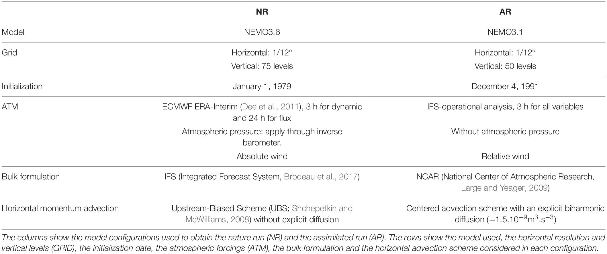
Table 1. Configurations of the nature run (NR) and assimilated run (AR).
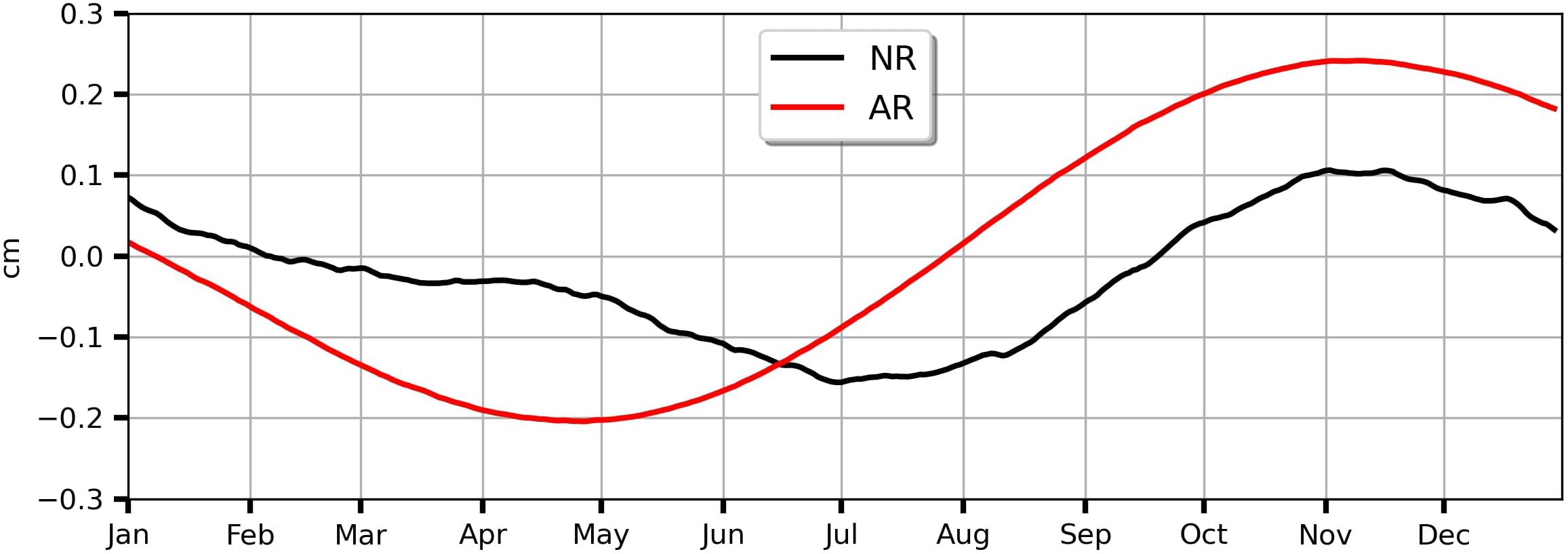
Figure 1. Time evolution of global mean of sea surface height (SSH, cm) for NR (black line) and AR (red line) over the period of January to December 2015.
To assess the impact of SWOT data, it was compared with conventional altimeter data from three nadir altimeters: Sentinel-3A (S3A), Sentinel-3B (S3B), and Jason-3 (J3). SWOT data was simulated from NR using the Jet Propulsion Laboratory’s (JPL) SWOT simulator (Gaultier et al., 2016). The simulator allows the adding of different types of errors to the SWOT data: KaRIn noise, roll error, phase error, timing error, baseline error, and wet tropospheric error (Gaultier et al., 2016). In this study, only KaRIn noise was considered. S3A, S3B, and J3 were sampled from NR by using their theoretical tracks with a resolution of 7 km between two points along the tracks. Theoretical tracks were used to overcome the problem of missing data. White noise with a standard deviation of 3 cm was simulated and added to those observations based on a random Gaussian distribution. Figure 2 shows the spatial coverage over 7 days (January 1–7, 2015) of J3 (Figure 2A), S3A (Figure 2B), S3B (Figure 2C), and the combination of the three satellites (Figure 2D). Figure 3 shows the SWOT sampling over the same time period.
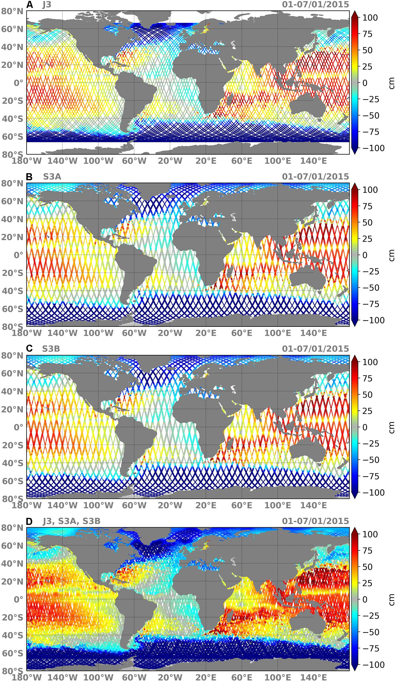
Figure 2. Tracks of Jason 3 (A), Sentinel 3A (B), Sentinel 3B (C), and a combination of the three satellites (D) over 7 days (January 1–7, 2015).
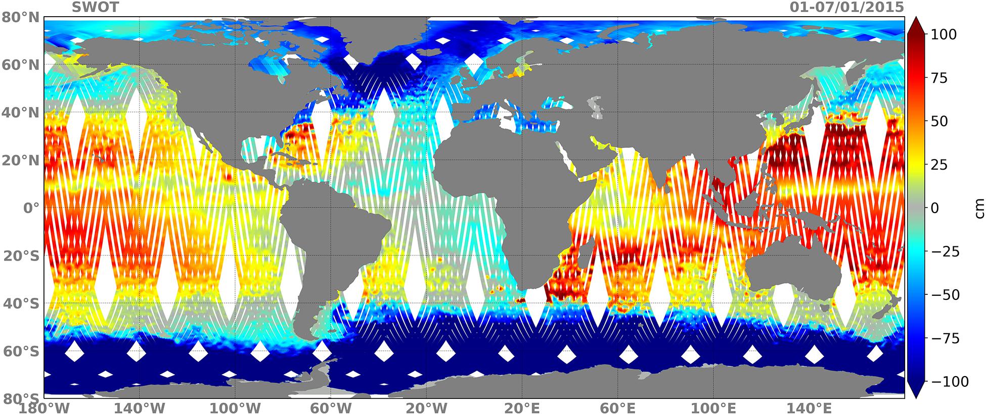
Figure 3. Global spatial coverage of SWOT SSH (cm) data over the period January 1–7, 2015.
Four different OSSEs (from OSSE0 to OSSE3) were carried out for this study. They are briefly summarized in Table 2. The OSSEs were conducted during the year 2015. They are differentiated by the types of data incorporated into each experiment. The OSSE0 (Free Run, hereafter FR) did not assimilate any observations. The OSSE1 assimilated the three nadir altimeter data, Sea Surface Temperature (SST) and in situ vertical profile of temperature (T) and salinity (S) at the same time and space positions as those of real observations that were available in 2015. The OSSE2 is similar to OSSE1 except that it assimilated SWOT data instead of nadir altimeter data. Finally, OSSE3 assimilated all observation types (combining SWOT and nadir altimeter data).
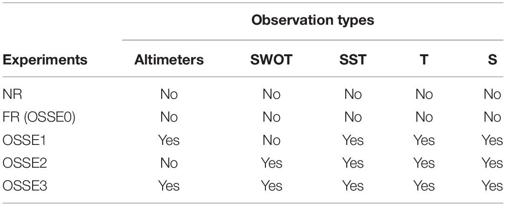
Table 2. Details of OSSEs differentiated by the observation types that were assimilated.
A common 3-month spin up was performed for all OSSEs from October 1 to December 31, 2014. During this spin up, observations were assimilated as in OSSE1. From January 1 to December 29, 2015, observations simulated from NR were assimilated as described in Table 2. The impact of data from SWOT and from nadir altimeters on SSH is first discussed in section “Impact on Sea Surface Height.” SSH error wavenumber spectra and coherence analyses are presented in section “Spectral Analysis of the SSH Error and Coherence.” Errors on temperature and salinity, both at the surface and at depth, are analyzed in section “Impact on Temperature and Salinity at Various Depths.” Section “Impact on Horizontal Currents” assesses the impact of SWOT data on the study of ocean circulation by evaluating the errors of zonal (U) and meridional (V) velocities at the surface and at depth. As there are no significant biases between the different OSSEs and the NR, only error variances are shown.
This section compares the SSH from each OSSE with the SSH from the NR. Figure 4 shows the spatial distribution of the variance of SSH in the NR. This variance was computed over the year 2015. As discussed in Benkiran et al. (2021), the SSH variance in the NR compares very well with real altimeter observations.
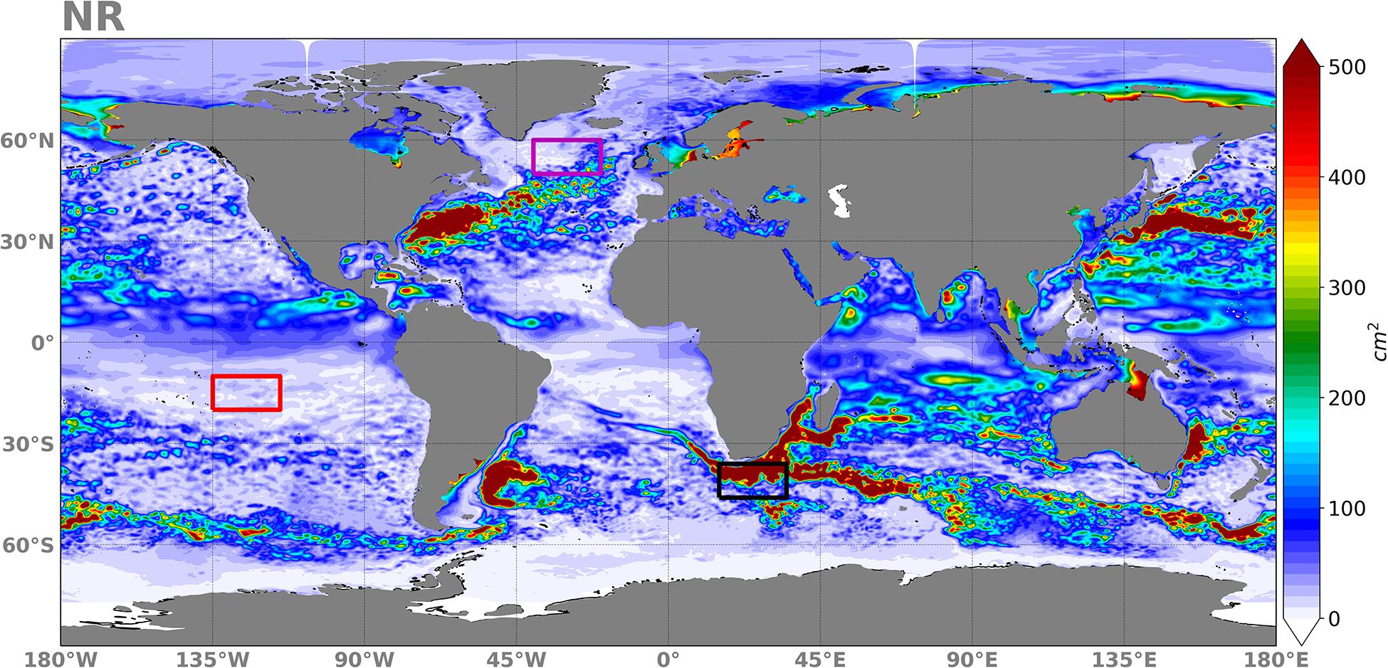
Figure 4. Variance of SSH (in cm2) in the NR over the period of January to December 2015. The purple, red, and black boxes denote the rectangle sub-regions for which wavenumber spectra and coherence analyses were performed.
To assess the results, the variance of SSH error between the NR and each OSSE for both analyses and 7-day forecasts (the assimilation cycle and sequence of analyses/forecasts is detailed in Lellouche et al., 2013) were computed globally for the period from January 1 to December 29, 2015. Results are shown in Figure 5. Even though the assimilation of the different observations started on October 1, 2014, the duration (3 months) of the spin up was not sufficient to stabilize the performance of the system for the year 2015. A decrease in errors was still observed from January 1, 2015 and the system converged towards a stable state by the end of February 2015. The FR error (OSSE0) oscillated around an error variance of 98 cm2 (Table 3). This error was reduced to 15 cm2 (17 cm2) in the OSSE1 for analyses (forecasts). The analysis and forecast error variances in OSSE2 are roughly equivalent to those of OSSE1. OSSE3 provided an improvement of 4 cm2 compared to OSSE1 for both analysis and forecast errors and its analysis (forecast) error variance oscillated around 11 cm2 (13 cm2). Apart from this figure, which was used to show what happened before March, all other results are indeed restricted to the period from March to December 2015.
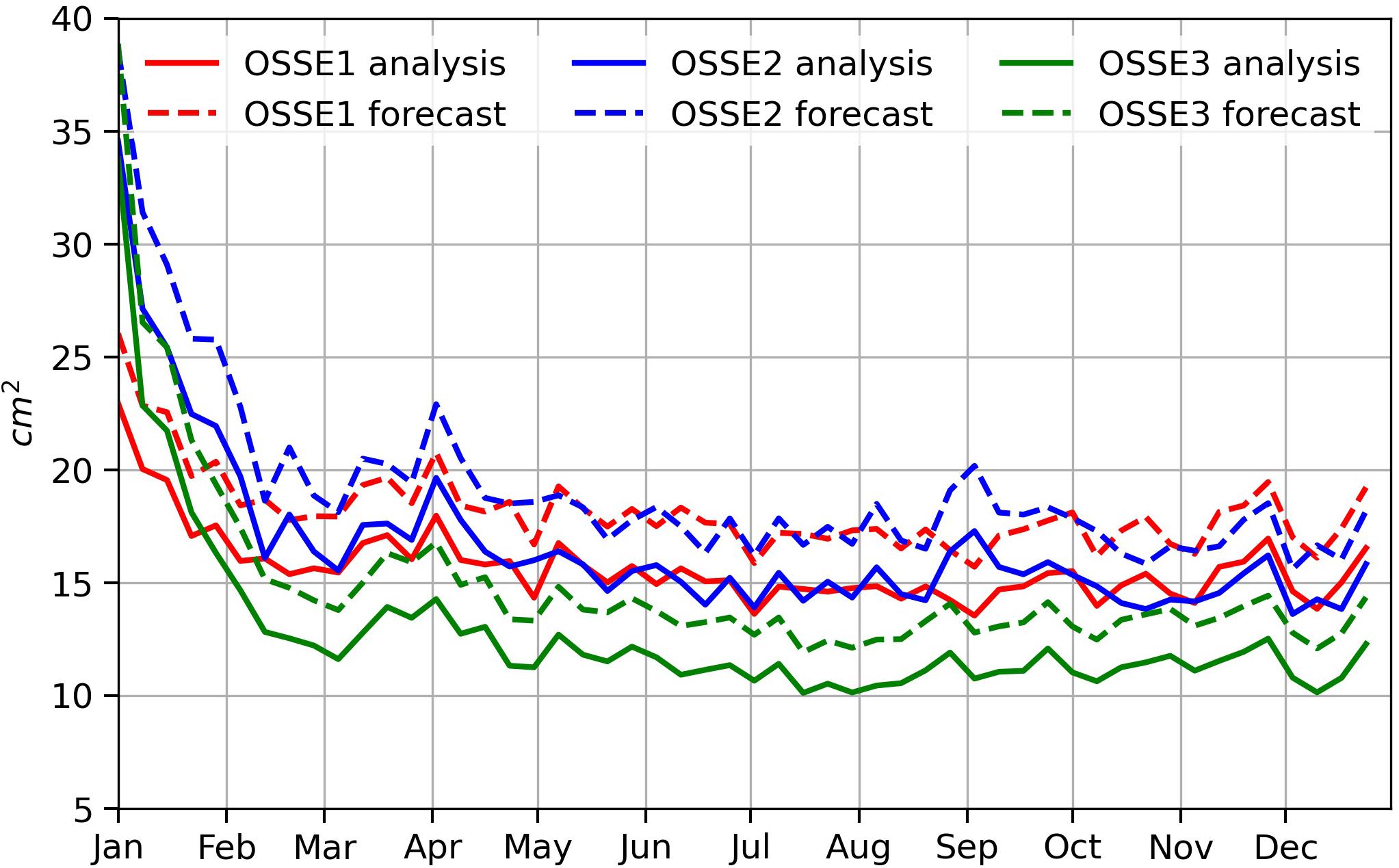
Figure 5. Temporal evolution of SSH error variance (in cm2) for 7-day ocean analysis (plain lines) and 7-day ocean forecast (dash lines) over the period from January 1 to December 29, 2015. The results were obtained by comparing the SSH in the OSSE1 (red lines), OSSE2 (blue lines), and OSSE3 (green lines) experiments with the SSH from the NR. See Table 2 for a description of each experiment.
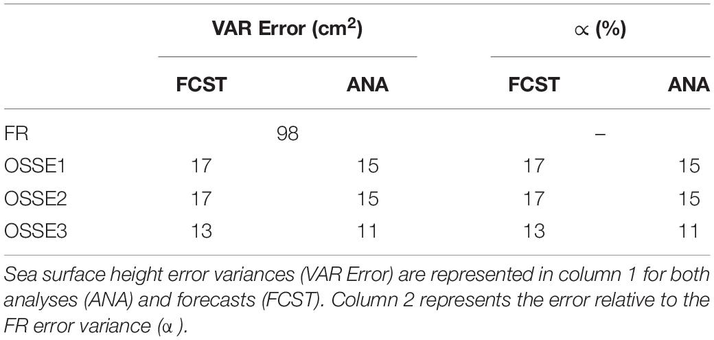
Table 3. Sea surface height ocean analysis and forecast error statistics over the period of March to December 2015.
The variance of SSH ocean analysis error for FR and the OSSE1 estimated from the difference between the AR and the NR is shown in Figures 6A,B, respectively. Figures 6C,D show the difference between the error variance of OSSE1 and that of OSSE2 and 3, respectively. Figure 6E shows the zonally averaged variance of SSH ocean analysis error. FR shows large differences with the NR especially in regions of large mesoscale variability (Figure 6A). This was expected because the mesoscale variability fields coming from the two models are uncorrelated due to the random nature of the eddy variability in the two models. Assimilation of data from three nadir altimeters led to a significant reduction of analysis error (Figure 6B). Assimilating SWOT data significantly reduced the error in high latitude regions, in the subtropical gyres and offshore of the western boundary currents (Figure 6C). The error was slightly higher in the core of high mesoscale variability regions and in the equatorial band (±10° of latitude), for assimilation of SWOT data than for assimilation of data from nadir altimeters. The joint assimilation of data from SWOT and nadir altimeters (Figure 6D) provided the best performance almost everywhere and showed a significant reduction or suppression of the degradation observed when SWOT alone is assimilated. This significant improvement of OSSE3 with respect to OSSE1 is also evidenced in the zonally averaged variance of SSH ocean analysis error (Figure 6E) particularly in the high-latitude regions, even though SWOT assimilation alone is less good than the assimilation of nadir altimeters at mid-latitudes where western boundary currents are located.
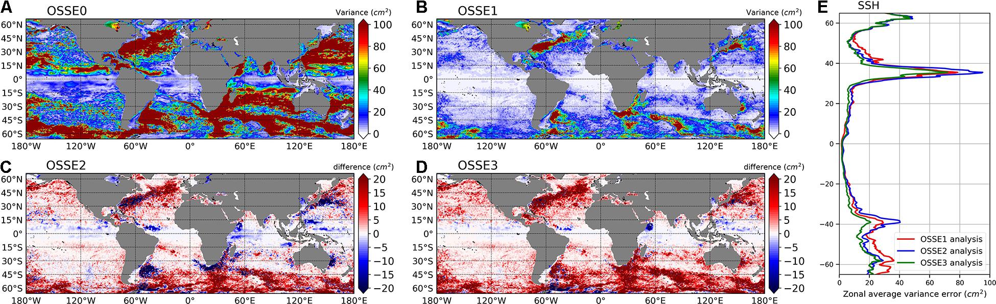
Figure 6. Global maps of SSH analysis error variance (in cm2) over the period of March to December 2015. The results were obtained by comparing the SSH of the NR with the SSH of the FR (A), and the ocean SSH analysis of the OSSE1 (B). (C,D) Difference between analysis error variance of OSSE1 and that of OSSE2 and OSSE3, respectively. Panel (E) shows the zonally averaged error variance of SSH for OSSE1 (red line), OSSE2 (blue line), and OSSE3 (green line).
To further analyze the results, the ratio of the variance of SSH error for a given OSSE and the FR (OSSE0) SSH error variance has been computed as:
where
is the temporal variance of SSH error obtained by comparing the NR with a given OSSE at a given location x and y over a period of t = 363 days with j = 1, 2, 3 referring to the j-th OSSE and nt referring to the maximum time. The results are presented in Table 3.
As expected, the OSSE0 error was consistently much higher than for any of the assimilated-data experiments. For the ARs, the forecast error variance was also always higher than the analysis error variance. The ratio ∝ for the analysis reached 15% for the OSSE1 and OSSE2. Combining data from SWOT and nadir altimeters (OSSE3) further reduced the errors by almost 26% with respect to OSSE1 or OSSE2.
SWOT is expected to make a great contribution in globally resolving features with wavelengths lower than 200 km that cannot be well represented with nadir altimeters (e.g., Le Traon et al., 2017). Figure 7 is similar to Figure 6 but for wavelengths lower than 200 km, and Table 4 summarizes the statistical results. The experiment assimilating only nadir altimeters (OSSE1) reduced the error by almost 38% compared to OSSE0 and its global mean value was 3.5 cm2. The assimilation of SWOT data (OSSE2) gave better results by reducing the error with respect to the OSSE1 by 0.5 cm2, which is almost a 47% and 15% decrease in error in comparison to OSSE0 and OSSE1, respectively. The improvement of OSSE2 over OSSE1 was observed everywhere in the global ocean. The error reduction was more accentuated in high-latitude regions, offshore of high mesoscale variability regions and subtropical gyres. Combining data from SWOT and nadir altimeters (OSSE3) further decreased the error variance. The error variance was reduced to 2.8 cm2 which is a 20% decrease in error over OSSE1. If we exclude the equatorial and tropical regions (±20°) where the signal below 200 km was quite small, the error reduction with respect to OSSE1 was more than 40%. The zonally averaged variance of SSH ocean analysis filtered at 200 km wavelength (Figure 7E) reflected the improvement of experiments assimilating SWOT data at all latitudes except the equatorial band where all the assimilated experiments performed the same. These results underline the impact of SWOT data in better representing small spatial scales.
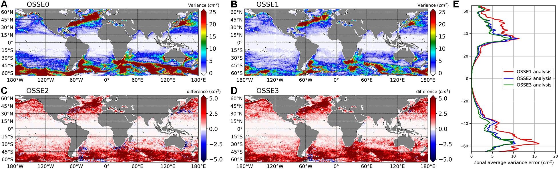
Figure 7. Global maps of SSH analysis error variance (in cm2) over the period of March to December 2015, and for structures below 200 km. The results were obtained by comparing the SSH of the NR with the SSH of the FR (A), and the ocean SSH analysis of the OSSE1 (B). (C,D) Difference between analysis error variance of OSSE1 and that of OSSE2 and OSSE3, respectively. Panel (E) shows the zonally averaged error variance of SSH for OSSE1 (red line), OSSE2 (blue line), and OSSE3 (green line).
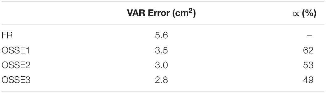
Table 4. Same as Table 3 but for SSH analysis filtered at wavelengths lower than 200 km.
In this section, we describe how wavenumber power spectral density (PSD) and spectral coherence for each OSSE are used to characterize the spatial structure of SSH analysis and forecast errors. Three areas of 10° in latitude by 20° in longitude were selected (see areas in Figure 4) to be representative of the low-latitude regions (red box), high eddy energy/mid-latitude regions (black box), and high-latitudes regions (purple box).
Wavenumber spectra (e.g., Dufau et al., 2016) were calculated from the daily zonal SSH error fields over a period from March 1 to December 29, 2015 by applying a Fast Fourier Transform. A Hanning window was applied to the data in order to reduce the leakage effect. Spectra were then averaged meridionally and temporally.
To quantify how the spatial scales of SSH signals are resolved in the different OSSEs, a spectral coherence (Thomson and Emery, 2014) was computed. The spectral coherence represents the correlation between two signals as a function of wavelength (Ubelmann et al., 2015). The spectral coherence between the SSH signal of OSSEs and NR is denoted in this study as Coh and is defined as follows:
where CSD represents the cross-spectral density, SD represents the spectral density and j refers to the j-th OSSE experiment.
Figure 8 shows the analysis (plain line) and forecast (dashed line) of mean SSH error spectra in a variance-preserving form (Thomson and Emery, 2014) (left panels) and the coherence between NR and each OSSE (right panels) for the three boxes represented in Figure 4.
Figure 8. Wavenumber spectra analysis (plains lines) and forecast (dash lines) of the SSH in the different OSSEs for the low-latitude region (red box; 135°W, 115°W; 20°S, 10°S) (A,B), mid-latitude region (black box; 15°E, 35°E; 46°S, 36°S) (C,D) and high-latitude region (purple box; 40°W, 20°W; 50°N, 60°N) (E,F) during the period of March to December 2015. The results are shown in the spectral window between 800 and 20 km for the OSSE0 (black lines), OSSE1 (red lines), OSSE2 (blue lines) and OSSE3 (green lines) experiments. (Left side) power spectra of SSH error with respect to NR, shown in a variance preserving form (cm2). (Right side) spectral coherence between the NR and each OSSE experiment.
In the three selected regions, differences among the OSSEs are shown by the error’s PSD (Figure 8, left panels). The forecast error was higher than the analysis error for all three assimilated experiments and all three regions. There was a clear decrease in the analysis error due to the assimilation of data from conventional altimeters (OSSE1) for the three regions except for the low-latitude region (Figure 8A) between 200 and 50 km of wavelength where the error in OSSE1 was higher compared to the FR error. For wavelengths below 200 km and at low-latitudes, altimeter noise was greater than the signal, and nadir altimeters tracks poorly sampled the signal. The assimilation system attempted to extrapolate the observation information and added (small scale) noise outside the tracks (see discussion in section 3.4.1 of Lellouche et al., 2018). SWOT data brought significant information in the low-latitude (Figure 8A) and high-latitude (Figure 8E) regions. In the mid-latitude region (Figure 8C), the error reduction was more important for OSSE1 than for the OSSE2 for wavelengths larger than 200 km. This may be because, due to its 21-day repeat period, SWOT sampling is less effective at constraining mesoscale signals in these highly energetic regions. The data assimilation system (see Benkiran et al., 2021) uses a 7-day window for both nadir altimeters and SWOT observations. This window is short for SWOT which has a repeat period of 21 days. Figure 3 shows that in a 7-day window, the SWOT sampling leaves large diamond-like areas unobserved, principally in mid-latitude regions. This means that in OSSE2, the SSH at these regions is not observed for one-third of the time (one assimilation cycle out of three). The application of smoother methods (e.g., Cosme et al., 2010) using future information to update the model’s state may provide a more accurate representation of the mesoscale variability. This would be useful for reanalysis and hindcasts. Finally combining data from SWOT and conventional altimeters reduced the analysis errors up to 100 km wavelength in the low-latitude region, 75 km wavelength in the mid-latitude region and 50 km wavelength in the high-latitude region.
Figure 8 (right panels) shows the result of spectral coherence for analysis (plain line) and forecast (dashed line) for the three selected regions. Differences between the assimilated OSSEs can be seen for wavelengths down to 75 km in the low-latitude region (Figure 8B), 50 km in the mid-latitude region (Figure 8D) and 50 km in the high-latitude region (Figure 8F). Considering 0.5 as the threshold for acceptable performance (effective resolution, see Ubelmann et al., 2015), OSSE3 had the best performances with an effective resolution down to 195 km for the low-latitude region, 179 km for the mid-latitude region, and 116 km for the high-latitude region. The coherence between the SSH signals in the ocean analysis was significantly increased in the low-latitude and high-latitude regions when assimilating SWOT data, compared to the assimilation of data from conventional altimeters. Considering the mid-latitude region, there was a very significant impact when combining data from both SWOT and conventional altimeters.
Another way to differentiate the errors produced by each OSSE in SSH fields, is to separate the wavenumber into two domains: small wavenumbers (large scales) constrained by available observations and large wavenumbers (small scales) that are unconstrained. The method used by D’Addezio et al. (2019) consists in normalizing the error spectrum of SSH fields. This normalization is defined as the ratio between the error spectrum of a given OSSE and the mean of the NR and the given OSSE spectra. It is defined as follows:
where εOSSE is the PSD of the SSH error with respect to the NR, γNR is the PSD of SSH in the NR, γOSSE is the PSD of SSH in a given OSSE and the brackets denote the mean of the two spectra.
Equation 3 gives the values of the normalized error spectrum and these values are in the range (0; 4). If the normalized value is 0 at a particular spatial scale, it implies that the SSH fields in the NR and the given OSSE share exactly the same features in that wavenumber. On the other hand, if the normalized value is 2 for a certain wavenumber, it implies that the SSH fields in the NR and the given OSSE are totally uncorrelated (NR and a given OSSE spectra have zero correlation); their features are totally unconstrained, and the assimilation has no impact on features at that spatial scale. A value larger than 2 means that the two fields are anticorrelated. A correlation of 0.5 between the SSH fields in the NR and the given OSSE equates to a normalized PSD of 1. This normalized PSD of 1 is defined as the separation threshold between the constrained and unconstrained spatial scales.
Figure 9 shows the normalized spectra of SSH analysis derived from the four OSSEs over low-latitude (Figure 9A), mid-latitude (Figure 9B), and high-latitude (Figure 9C) regions. The regions are all represented in Figure 4. There are large differences between each experiment and each region. For all the three regions, OSSE2 produced lower errors than OSSE1 and crossed the normalized PSD threshold of 1 at smaller wavelengths than OSSE1. OSSE3 had the lowest errors in all the three regions and crossed the normalized PSD threshold of 1 at lower wavelengths than the other OSSEs.
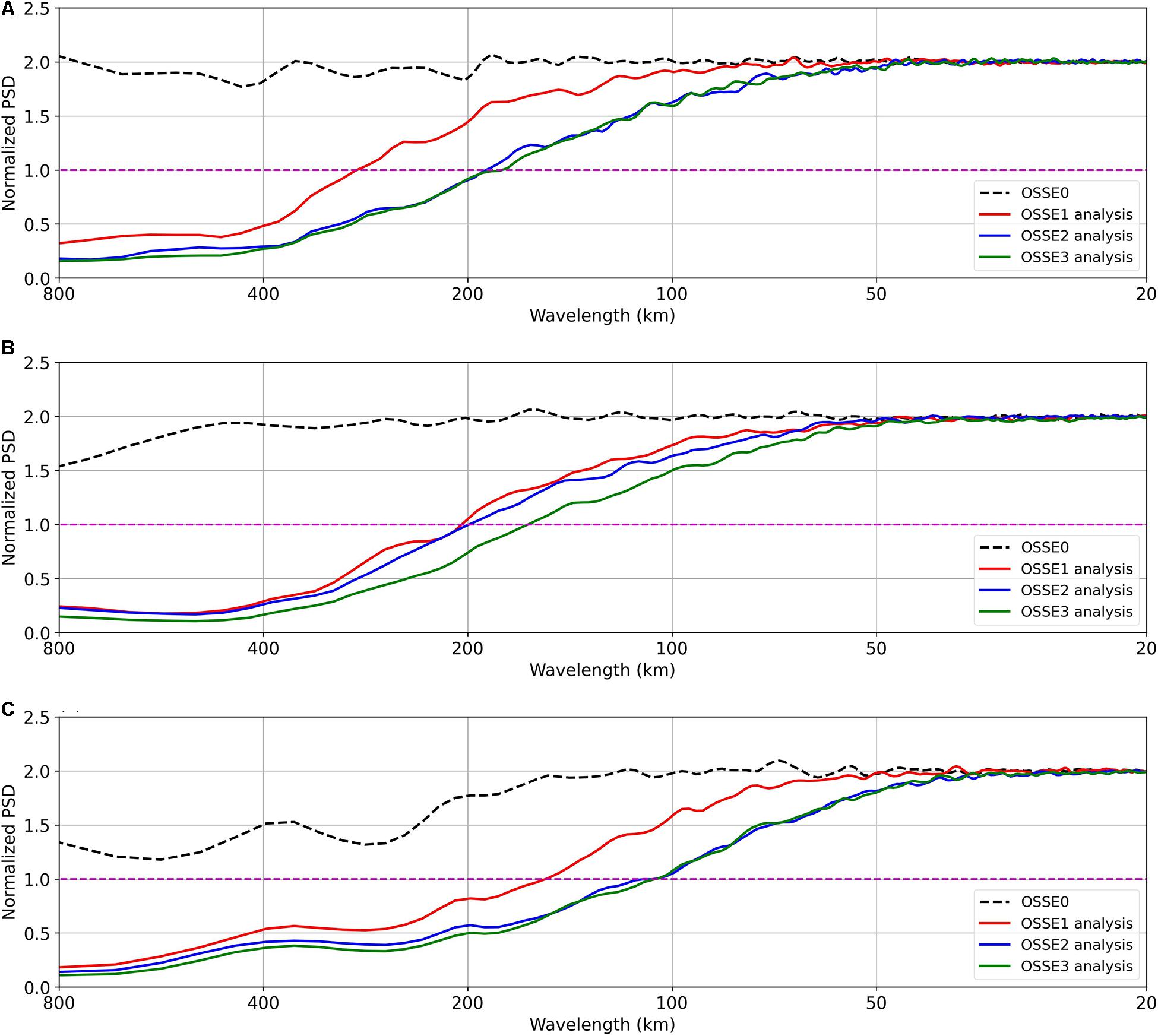
Figure 9. Normalized wavenumber SSH error spectra of (A) low-latitude region (red box), (B) mid-latitude (black box), and (C) high-latitude (purple box) over the period of March to December 2015. See Eq. 3 for more information on the normalization scheme. All the three regions are depicted in the Figure 4.
Table 5 gives the wavelength at which each OSSE crossed the normalized PSD threshold of 1. For the high-latitude region, OSSE1 constrained the wavelengths down to 152 km. Both OSSE2 and OSSE3 constrained the wavelengths down to 101 km. This result highlights the fact that the experiments assimilating data from SWOT (OSSE2) and data from SWOT and nadir altimeters (OSSE3) constrained an additional 51 km over the OSSE1, which assimilates only data from nadir altimeters. In the low-latitude region, OSSE1 constrained the wavelengths down to 281 km; OSSE2 constrained the wavelengths down to 184 km and OSSE3 constrained the smallest wavelengths down to 174 km. Finally, when considering the mid-latitude region, OSSE3 again produced the lowest minimum constrained wavelength of 157 km. In each selected region, the OSSE3 produced the smallest minimum constrained wavelength with the smallest value in the high-latitude region followed by the mid-latitude region and the low-latitude region.
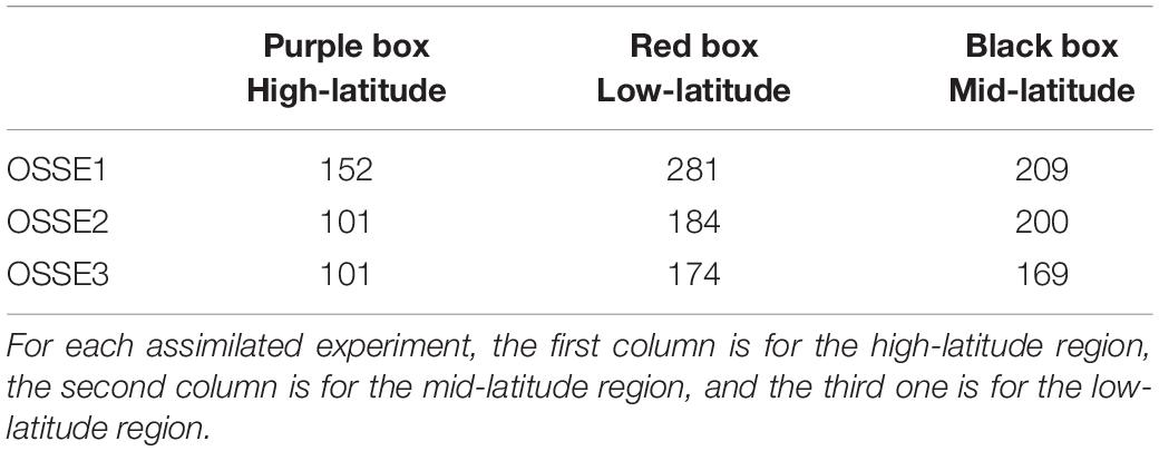
Table 5. Minimum constrained wavelength (km, normalized PSD = 1) for each experiment and for different geographical areas.
In order to assess the impact of SWOT data at small scales with respect to data from nadir altimeters, the percentage of the decrease of the error (here for ocean analysis only) compared to the OSSE1 in the range of 200 to 50 km wavelength is evaluated by:
where kmin (kmax) is the wavelength of 50 km (200 km) and j = 2, 3 refers to the jth experiment. A value of zero means that, on average, the jth experiment and OSSE1 produce similar spectra in the selected wavelength range. A summary of the percentage decrease in the considered wavelengths for the three selected regions is given in Table 6. For the high-latitude region, OSSE2 gave a 47% decrease in error over OSSE1 and a reduction of 49% occurred for OSSE3 compared to OSSE1. Low-latitude region shows that both the experiments assimilating SWOT data (OSSE2 and OSSE3) performed best with a 65% decrease in error in comparison to OSSE1. The mid-latitude region had the smallest error reduction; the reduction in error in the OSSE2 and OSSE3 was 5 and 33% compared to OSSE1. Overall, experiments that assimilated SWOT data (OSSE2 and OSSE3) showed a clear improvement in retrieving small scales as compared to OSSE1. The results demonstrate that the data assimilation system (Benkiran et al., 2021) enables the extraction of useful information from the mesoscale down to the smaller scales when SWOT data are assimilated and even more so when data from SWOT and nadir altimeters are jointly assimilated.
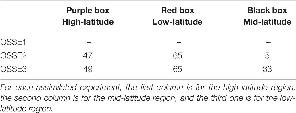
Table 6. Reduction of the SSH error in the ocean analysis with respect to OSSE1 for wavelengths between 200 and 50 km for each experiment and for the three different geographical areas.
Our global OSSE results compare well with Bonaduce et al. (2018) and D’Addezio et al. (2019) results. In Bonaduce et al. (2018), at the correlation of 0.6, the minimum constrained wavelength was 125 km for the experiment assimilating both nadir and wide-swath observations which is 5 km above the value found for our experiment assimilating both nadir and SWOT observations. Note that Bonaduce et al. (2018) analyzed the impact of a different concept of wide-swath altimetry with a less stringent noise requirement in comparison to SWOT. Despite the differences in the OSSE designs (observation noise, forcing fields and choice of NR and FR), almost the same results were found. Considering D’Addezio et al. (2019), the minimum constrained wavelength (correlation = 0.5) reported was 139 km for the experiment assimilating both nadir and SWOT observations instead of 167 km in our study. This difference is very likely due to differences in OSSE designs. In particular, D’Addezio et al. (2019) used a very high-resolution model (1 km horizontal resolution) for the NR and the AR, while we used a 1/12° resolution model.
To sum up, the results highlight that (i) combining SWOT and nadir altimeters in a data assimilation system gives the smallest minimum constrained wavelength and (ii) the impact is greater in the high-latitude region where SWOT observations provide better spatio/temporal coverage.
This section aims to verify that better constraining the SSH fields does not degrade the results for temperature and salinity. Figure 10 shows the mean standard deviation of the analysis of both temperature (Figure 10A) and salinity (Figure 10B) errors as a function of depth for the global ocean, calculated over the period from March to December 2015. The temperature profile shows a maximum error at the depth of the thermocline (around 100 m). The OSSE1 outperformed the OSSE2 experiment at that depth. The three assimilated experiments errors were roughly equivalent for the top 75 m of the water column. Assimilating SWOT data (OSSE2) led to an improvement over the entire water column below 100 m compared with the OSSE1. OSSE3, which assimilates all the available data, outperformed all the other OSSEs below the 75 m of the water column and then converged with the OSSE2 experiment at a greater depth. The salinity profile shows that the error decreases with depth. Globally, the OSSE1 error levels were roughly equivalent to those of the OSSE2 and OSSE3 experiments, and converged to the error of 0.02 psu at a depth of 1000 m. Note that the salinity field is less impacted by the assimilation system than the temperature field. As explained by Verrier et al. (2017), SSH represents an integral of the density anomaly and since density variations are mainly correlated to temperature variations and less to salinity variations in most ocean regions, the impact of SSH assimilation is more pronounced in temperature than in salinity.
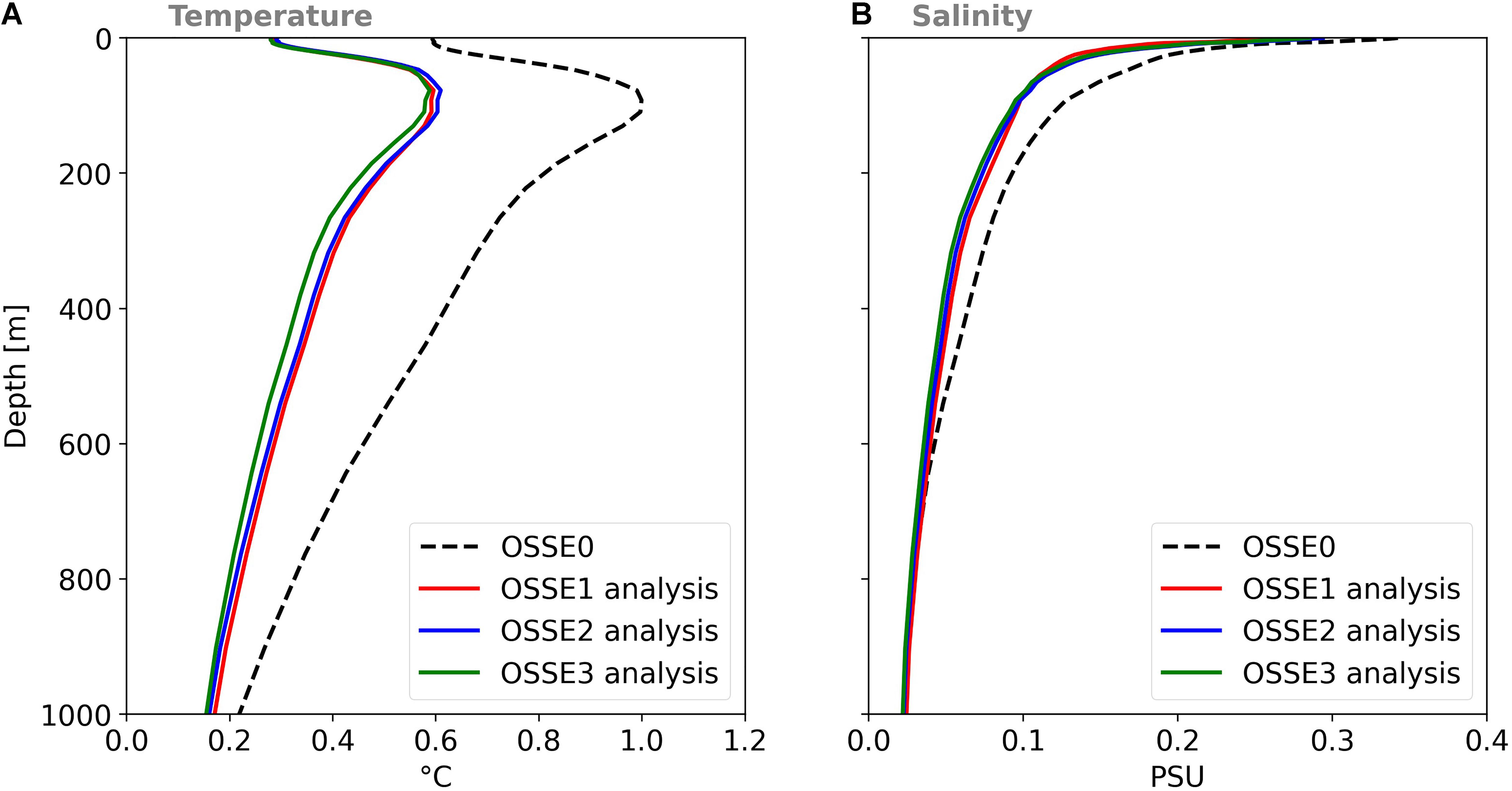
Figure 10. Globally averaged standard deviation of temperature errors (A) and salinity errors (B) as a function of depth. Results are obtained by comparing temperature and salinity in the FR (dash black line), OSSE1 (red lines), OSSE2 (blue lines), and OSSE3 (green lines) with temperature and salinity from the NR over the period of March to December 2015. Units are in °C for temperature and psu for salinity.
This section compares the impact of SWOT data on representing the surface horizontal ocean currents for both ocean analyses and forecasts. Zonal (U) and meridional (V) currents are non-assimilated model variables, and they play a key role in ocean applications. It is thus interesting to analyze the way in which they are improved when assimilating SWOT data.
Figure 11 shows a time series of the global error variance for the 7-day analysis and forecast of both U (Figure 11A) and V (Figure 11B) at the surface. The two plots similarly show a seasonal variation in errors with a peak in summer for all OSSEs. This can be explained by the seasonal variability observed in the surface eddy kinetic energy (EKE) with a broad maximum in summer (e.g., Rieck et al., 2015). The variance of errors decreased from OSSE1 to OSSE3. As expected, the analysis error in each assimilated OSSE was reduced compared to the forecast error. Importantly, the OSSE3 forecast error was smaller than the analysis error in OSSE1 and OSSE2 for both U and V velocities. This is evidence that combining data from SWOT with data from nadir altimeters will improve forecasting techniques.
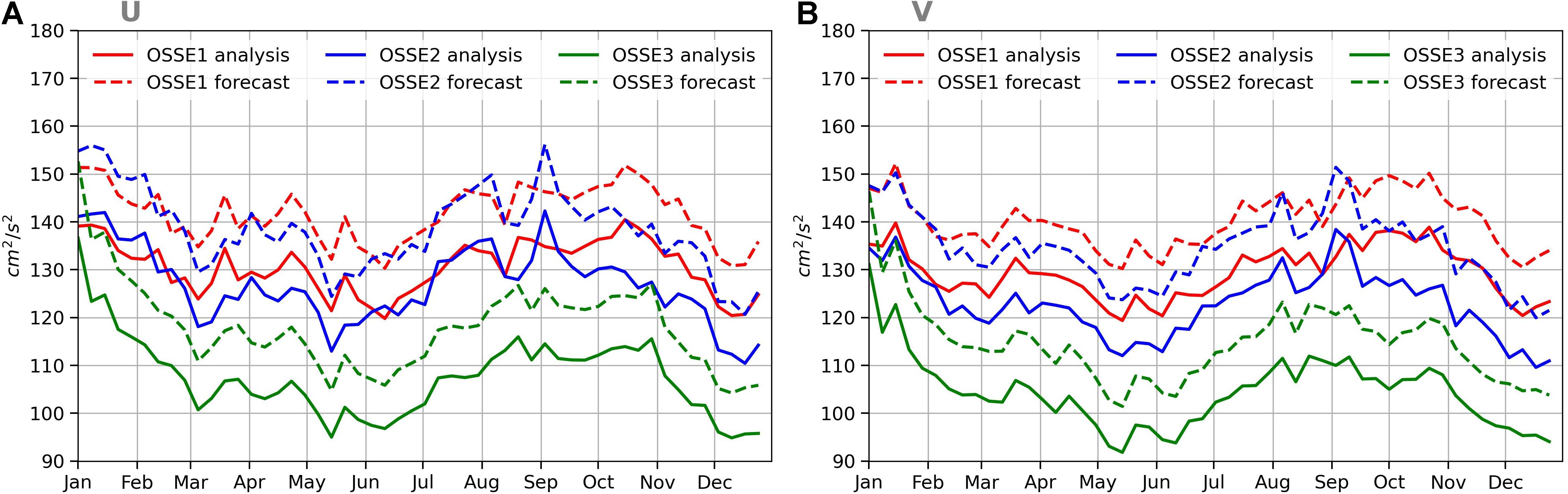
Figure 11. Temporal evolution of (A) zonal velocity (U) and (B) meridional velocity (V) error variance (in cm2/s2) for 7-day ocean analysis (plain lines) and 7-day ocean forecast (dash lines) over the period from January 1 to December 29, 2015. The results were obtained by comparing U and V in the OSSE1 (red lines), OSSE2 (blue lines), and OSSE3 (green lines) experiments with the U and V from the NR. See Table 2 for a description of each experiment.
Figures 12A,B respectively show a global maps of analysis error variance of zonal velocity for OSSE0 and 1. Figures 12C,D show the difference between the analysis error variance of OSSE1 and that of OSSE2 and 3, respectively. Figure 12E shows the zonally averaged variance of U velocity ocean analysis error. OSSE0 shows high values everywhere for the velocity variances. Assimilation of data from three nadir altimeters (Figure 12B) led to a significant reduction of the analysis error in comparison to OSSE0. Assimilating SWOT data (Figure 12C) reduced the error in the polar regions, offshore of the high mesoscale variability regions and the subtropical gyre regions compared to OSSE1. In the core of high mesoscale variability regions, the SWOT (OSSE2) error was higher than the error obtained with data from three nadir altimeters (OSSE1). This result is probably related to the poor temporal sampling of SWOT, which does not improve control of the fast-evolving mesoscale variability. Similarly, in the equatorial band, fast ocean dynamics dominate, and the assimilation of SWOT data alone is less efficient than for the three nadir altimeters. However, the impact of assimilating data from SWOT and nadir altimeters (Figure 12D) remained positive almost everywhere, except in the equatorial band where a slight degradation remained. The improvement of experiments assimilating SWOT data (OSSE2 and OSSE3) with respect to experiment assimilating only nadir altimeters data (OSSE1) is also evidenced in the zonally averaged variance of U ocean analysis (Figure 12E) at all latitudes except in the equatorial band. Similar results were obtained with the meridional velocity (not shown).
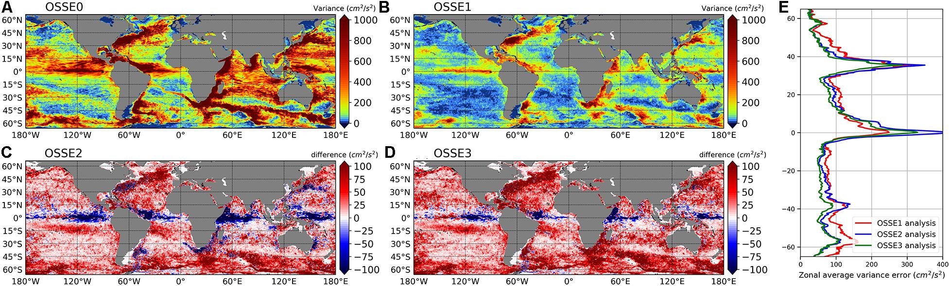
Figure 12. Maps of zonal velocity (U) analysis error variance over the period of March to December 2015. The results were obtained by comparing the NR zonal velocity with the analysis of the FR (A) and OSSE1 (B). (C,D) Difference between analysis error variance of OSSE1 and that of OSSE2, and OSSE3, respectively. Panel (E) shows the zonally averaged error variance of U for OSSE1 (red line), OSSE2 (blue line), and OSSE3 (green line). Units are in cm2/s2.
The same scores as the one used for the SSH (Table 3) are shown in Table 7 for surface zonal (U) velocity and for both analysis and forecast. U and V (not shown here) statistics are almost similar. OSSE1 globally averaged analysis error variance of U was 130 cm2/s2 and represents 32% of the FR error variance. Compared to OSSE1, an analysis error variance reduction of 5 cm2/s2 was found for OSSE2 and of 25 cm2/s2 for OSSE3. These statistics demonstrate that the assimilation of SWOT data better constrains surface velocity fields and that the combination of data from SWOT plus nadir altimeters performs best with almost a 20% decrease in analysis error over OSSE1. Assimilation of SWOT data does indeed improve the zonal and meridional velocities of the entire water column. This can be seen in Figure 13, which shows the globally averaged velocity analysis error variance as a function of depth. As expected, the error of both components decreased with depth for all experiments. OSSE2 yielded a lower error over the entire water column as compared to OSSE1. The best experiment was the OSSE3 which had a positive impact down to the depth of 1000 m and which outperformed all the other OSSEs.
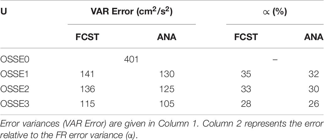
Table 7. Global statistics of zonal (U) velocity error variance for both analysis (ANA) and forecast (FCST) over the period of March to December 2015.
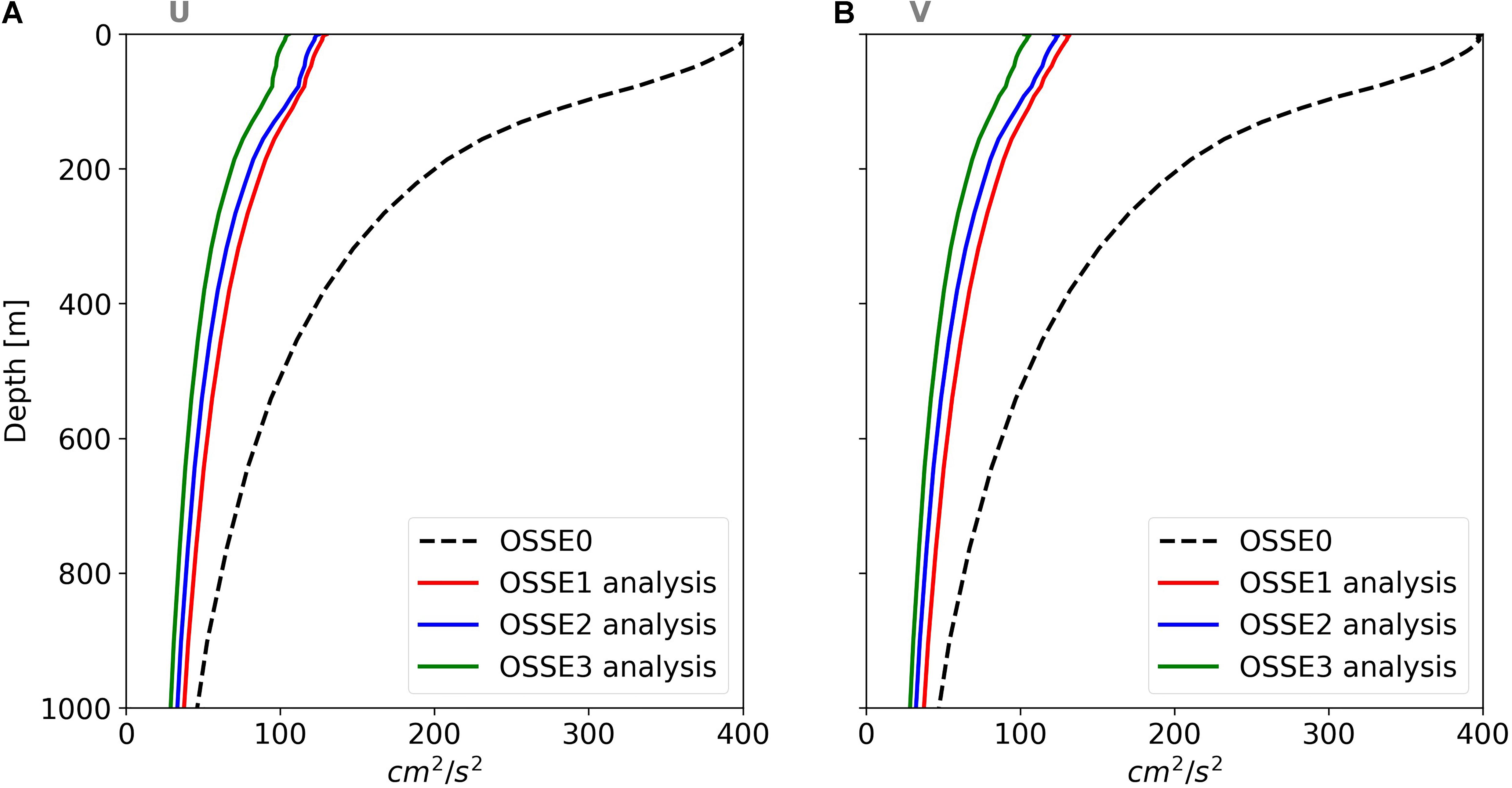
Figure 13. Globally averaged error variance for (A) zonal and (B) meridional velocities (in cm2/s2) over the period of March to December 2015. The results were obtained by comparing zonal and meridional velocities in the FR (dash black line), OSSE1 (red lines), OSSE2 (blue lines), and OSSE3 (green lines) with zonal and meridional velocities from the NR.
Key operational oceanography applications such as for search and rescue or pollutant dispersal rely on a good model representation of the lateral stirring and mixing of the ocean, processes that are dominated by the mesoscale, a spatial range which should be improved when SWOT altimetry observations are assimilated in ocean models, through better constraining of mesoscale structures.
Lagrangian analysis, through particle tracking, is a powerful tool for evaluating lateral transport in ocean models. In this section we evaluate the OSSEs’ skills in reproducing the particle drift observed in the NR, which is very similar to that used when validating operational ocean products with surface drifters (Liu and Weisberg, 2011; Sotillo et al., 2016). Lagrangian particles are initialized within each grid cell of the native 1/12° ORCA grid between latitudes of 66°S and 66°N for a single release on May 7, 2015, and subsequently advected horizontally for 7 days by the NR daily mean surface velocity field, to obtain the “True” particle trajectories. The Lagrangian experiment is then repeated, but using the OSSE velocity field instead. As such, for each grid cell we obtain four trajectories: that of the NR and one for each OSSE. In total approximately 5,448,000 particles were deployed for each experiment. The Lagrangian experiments were carried out using the Ariane software (Blanke and Raynaud, 1997). The ±66° of latitude was used as this is the inclination and maximum latitude of the Jason orbit.
To assess the OSSEs’ skills in reproducing the Lagrangian transport observed in the NR we calculated the separation distance between particles released in the OSSEs with their equivalent released in the NR, after 7 days (Barron et al., 2007). The separation distance for OSSE1 is shown in Figure 14A. For OSSE2 and OSSE3, Figures 14B,C, respectively, show the change in separation distance relative to OSSE1. Assimilation of SWOT data improves the surface Lagrangian lateral transport of OSSEs (Figure 14D): using surface velocities of either OSSE2 or OSSE3 (both assimilating SWOT), lower separation distance between OSSE particles and their NR equivalent is found than when using velocities of OSSE1 (assimilating nadir only). The median value for the separation distance after 7 days in OSSE1 (three nadir) was 44 km; in OSSE2 (SWOT), 36 km, and in OSSE3 (SWOT + three nadir), 34 km. A more meaningful statistic is the proportion of particles within 50 km of its equivalent in the NR; this value increased from 56% in OSSE1 to 64 and 67% in OSSE2 and OSSE3, corresponding respectively to an improvement of 18 and 19% relative to OSSE1 (Table 8). For OSSE2, the improvement relative to OSSE1 was overall global (Figure 14B), except for the regions along the equator and, to a lesser extent, the western boundary current regions that showed no improvement or some minor degradation (e.g., Agulhas, Gulf Stream, and Kuroshio regions). However, when data from SWOT was coupled with three nadir observations (OSSE3) degradations were significantly reduced or suppressed with only the equatorial band as a region in which some moderate degradation remained (Figure 14C).
Figure 14. Separation distance between particles deployed in OSSE1 (three nadir) and their equivalent in the NR after 7 days of advection by their respective surface current velocities (A). The results were averages in 2 × 2 degree bins. (B,C) Changes (in %) of the separation distance when using OSSE2 (SWOT) or OSSE3 (SWOT + three nadir) surface velocities relative to results with OSSE1. (D) Binned histogram of separation distance for all OSSEs globally.
Table 8. Summary of statistics for the separation distance of OSSE Lagrangian particles with their NR equivalent after 7 days of advection, for the global ocean and three boxes for the high-latitude, mid-latitude, and low-latitude regions.
For areas typical of low-latitude, mid-latitude, and high-latitude regions all represented on the Figure 4, an improvement was found for OSSE2 and OSSE3 in lateral transport, with a smaller separation distance between their particles and their NR equivalent as compared to OSSE1 (Figure 15). This was most pronounced for the mid-latitude region with an improvement relative to OSSE1 of 35 and 42 % for OSSE2 and OSSE3, respectively (Table 8). Note also the difference in OSSE results for the different regions, with ∼60% of particles within 50 km for low-latitude region, or high-latitude region and only ∼30–40% for the mid-latitude region.
Figure 15. Same as Figure 14D but focusing on the three regions representative of the (A) low-latitude region (red box; 135°W, 115°W; 20°S, 10°S), (B) mid-latitude region (black box; 15°E, 35°E; 46°S, 36°S), and (C) high-latitude region (purple box; 40°W, 20°W; 50°N, 60°N), respectively.
A first attempt was made to quantify the impact of SWOT swath altimeter data together with data from conventional nadir altimeters in a global high-resolution analysis and forecasting system. The OSSE framework, discussed in Benkiran et al. (2021), relies on two global 1/12° models with different physics and forcing being used for the NR (“truth” used to simulate observations) and the AR (where the simulated observations are assimilated). The data assimilation system with the updates described in Benkiran et al. (2021) is the one that will be used operationally at MO for the Copernicus Marine Service from the end of 2021.
The impact of SWOT data together with that from conventional altimeters is quantified by calculating analysis and forecast error variances for SSH, temperature, salinity, and zonal and meridional velocities. In addition, wavenumber and coherence spectral analyses of SSH errors and Lagrangian transport errors are also computed.
Surface Water Ocean Topography will have a strong impact on the quality of ocean analysis and forecasts. Adding SWOT observations to those from three conventional altimeters globally reduces the variance of SSH and velocity analysis and forecast errors by about 30 and 20%, respectively. Improvements are greater for wavelengths below 200 km (larger than 40% outside tropical regions) and in high-latitude regions where the spatio-temporal coverage of SWOT is much denser. A large impact has also been observed in high mesoscale variability regions but data from SWOT alone does not yield better results than data from three nadir altimeters. This may be explained by the poor time sampling of SWOT observations which does not constrain these highly dynamic areas. This result could also be related to important differences between the NR and the AR in these regions (see discussion in Benkiran et al., 2021). When simulated observations from the NR are not consistent with the AR model dynamics, this limits the AR’s ability to get closer to the NR.
Wavenumber and coherence spectral analysis of errors were carried out in three regions representative of low-latitude, mid-latitude and high-latitude regions. The results showed that the experiments assimilating SWOT data (OSSE2 and OSSE3) consistently produced lower errors for wavelengths larger than 100 km compared to the experiment that assimilated only nadir altimeter data (OSSE1). The improvements are greater in high-latitude regions where space/time coverage of SWOT is much denser. The minimum constrained wavelength was 152 km for the OSSE1 as opposed to 101 km for OSSE2 and OSSE3. This significant improvement shows the high potential of SWOT data assimilation to better constrain ocean analysis and forecasting models. These results are consistent with those found with Lagrangian analysis, which shows that the assimilation of data from SWOT and data from SWOT plus nadir altimeters globally improves the Lagrangian lateral transport at the surface, reducing the separation between OSSE particles with their NR equivalent.
Our results are consistent with previous studies carried out at regional scales (Bonaduce et al., 2018; D’Addezio et al., 2019). They confirm the potential of SWOT data for ocean analysis. They also show that the impact of SWOT data can be very different depending on geographical areas.
It is expected that improvements in the data assimilation system could lead to a stronger positive impact of SWOT data. The background error covariance is based on the statistics of a collection of 3D ocean state anomalies computed from a long numerical experiment with respect to a running mean in order to estimate the 7-day scale error on the ocean state at a given period of the year (see Lellouche et al., 2013 for more details). These anomalies were derived from the MO GLORYS12 reanalysis at 1/12° covering the altimetry era from 1992 onward. Even though the construction of these anomalies has been optimized in Benkiran et al. (2021) in order to better assimilate data that contain mesoscale structures, they do not represent the true model errors which in our case would be the differences between the AR and the NR. The model error characterization could thus be improved through a refined set of anomalies. Two improvements under investigation are multiscale data assimilation and a smoother version of the data assimilation system. Both are being tested. The first is expected to better constrain the small scales; the second enhances the observability at mid-latitudes. Future studies should also take into account the KaRIn instrument noise dependency to waves. They should also take into account the full error spectrum considering the impact of Level 2 to Level 3 pre-processing steps (crossover minimization and cross-calibration with conventional nadir altimeters).
Although this is only a first step, the study has demonstrated that future SWOT data could be readily assimilated in the forthcoming Copernicus Marine Service global high-resolution analysis and forecasting system, with a positive impact everywhere and with very good performances.
The main limitation of SWOT is related to its long-time repeat period. On the longer run, flying a constellation of two wide swath altimeters (i.e., reducing the time repeat period by 2) would thus be highly beneficial to further improve the performances, in particular, for the small space and time scales. This has been analyzed in a dedicated study carried out for European Space Agency (ESA) in the framework on the long-term evolution of the Copernicus Sentinel 3 constellation. Results will be reported in a separate article.
The raw data supporting the conclusions of this article will be made available by the authors, without undue reservation.
BT conducted all the analyses of OSSEs and wrote the manuscript. MB set up the scientific protocol of OSSEs, performed the simulation, and made the first analyses of the results. P-YL wrote the introduction and conclusion and reviewed the whole manuscript. SJ carried out the Lagrangian diagnostics and wrote the corresponding section. JL and GR commented on a preliminary version of the manuscript. All authors contributed to the article and approved the submitted version.
This study was funded under a CNES (French Space Agency) and Mercator Ocean partnership agreement.
The authors declare that the research was conducted in the absence of any commercial or financial relationships that could be construed as a potential conflict of interest.
All claims expressed in this article are solely those of the authors and do not necessarily represent those of their affiliated organizations, or those of the publisher, the editors and the reviewers. Any product that may be evaluated in this article, or claim that may be made by its manufacturer, is not guaranteed or endorsed by the publisher.
Barron, C. N., Smedstad, L. F., Dastugue, J. M., and Smedstad, O. M. (2007). Evaluation of ocean models using observed and simulated drifter trajectories: impact of sea surface height on synthetic profiles for data assimilation. J. Geophys. Res. Oceans 112:12.
Benkiran, M., Ruggiero, G., Greiner, E., Le Traon, P.-Y., Rémy, E., Lellouche, J. M., et al. (2021). Assessing the impact of the assimilation of SWOT observations in a global high-resolution analysis and forecasting system. Part 1: method. Front. Mar. Sci. 8:691955. doi: 10.3389/fmars.2021.691955
Blanke, B., and Raynaud, S. (1997). Kinematics of the Pacific equatorial undercurrent: an eulerian and lagrangian approach from GCM results. J. Phys. Oceanogr. 27, 1038–1053.
Bloom, S. C., Takacs, L. L., da Silva, A. M., and Ledvina, D. (1996). Data assimilation using incremental analysis updates. Mon. Weather Rev. 124, 1256–1271. doi: 10.1175/1520-0493(1996)124<1256:DAUIAU>2.0.CO;2
Bonaduce, A., Benkiran, M., Remy, E., Le Traon, P. Y., and Garric, G. (2018). Contribution of future wide-swath altimetry missions to ocean analysis and forecasting. Ocean Sci. 14, 1405–1421. doi: 10.5194/os-14-1405-2018
Brodeau, L., Barnier, B., Gulev, S. K., and Woods, C. (2017). Climatologically significant effects of some approximations in the bulk parameterizations of turbulent air–sea fluxes. J. Phys. Oceanogr. 47, 5–28. doi: 10.1175/JPO-D-16-0169.1
Cosme, E., Brankart, J.-M., Verron, J., Brasseur, P., and Krysta, M. (2010). Implementation of a reduced rank square-root smoother for high resolutionocean data assimilation. Ocean Model. 33, 87–100. doi: 10.1016/j.ocemod.2009.12.004
D’Addezio, J. M., Smith, S., Jacobs, G. A., Helber, R. W., Rowley, C., Souopgui, I., et al. (2019). Quantifying wavelengths constrained by simulated SWOT observations in a submesoscale resolving ocean analysis/forecasting system. Ocean Model. 135, 40–55. doi: 10.1016/j.ocemod.2019.02.001
Dee, D. P., Uppala, S. M., Simmons, A. J., Berrisford, P., Poli, P., Kobayashi, S., et al. (2011). The ERA-Interim reanalysis: configuration and performance of the data assimilation system. Q. J. R. Meteorol. Soc. 137, 553–597. doi: 10.1002/qj.828
Dufau, C., Orsztynowicz, M., Dibarboure, G., Morrow, R., and Le Traon, P. Y. (2016). Mesoscale resolution capability of altimetry: present and future. J. Geophys. Res. Oceans 121, 4910–4927. doi: 10.1002/2015JC010904
Fu, L.-L., Alsdorf, D., Rodriguez, E., Morrow, R., Mognard, N., Lambin, J., et al. (2009). “The SWOT (surface water and ocean topography) mission: spaceborne radar interferometry for oceanographic and hydrological applications,” in Proceedings of the OCEANOBS’09 Conference (Venice-Lido), Venice-Lido.
Gaultier, L., Ubelmann, C., and Fu, L.-L. (2016). The challenge of using future SWOT data for oceanic field reconstruction. J. Atmos. Ocean. Tech. 33, 119–126. doi: 10.1175/JTECH-D-15-0160.1
Halliwell, G. R., Srinivasan, A., Kourafalou, V., Yang, H., Willey, D., Hénaff, M. L., et al. (2014). Rigorous evaluation of a fraternal twin ocean osse system for the open Gulf of Mexico. J. Atmos. Ocean. Tech. 31, 105–130. doi: 10.1175/JTECH-D-13-00011.1
Hamon, M., Greiner, E., Le Traon, P. Y., and Remy, E. (2019). Impact of multiple altimeter data and mean dynamic topography in a global analysis and forecasting system. J. Atmos. Ocean. Technol. 36, 1255–1266. doi: 10.1175/JTECH-D-18-0236.1
Hoffman, R. N., and Atlas, R. (2016). Future observing system simulation experiments. Bull. Am. Meteorol. Soc. 97, 1601–1616. doi: 10.1175/BAMS-D-15-00200.1
Klein, P., Lapeyre, G., Siegelman, L., Qiu, B., Fu, L. L., Torres, H., et al. (2019). Ocean-Scale interactions from space. Earth Space Sci. 6, 795-817. doi: 10.1029/2018EA000492
Large, W. G., and Yeager, S. G. (2009). The global climatology of an interannually varying air–sea flux data set. Clim. Dynam. 33, 341–364. doi: 10.1007/s00382-008-0441-3
Le Traon, P. Y., Dibarboure, G., Jacobs, G., Martin, M., Remy, E., and Schiller, A. (2017). “Use of satellite altimetry for operational oceanography,” in Satellite Altimetry Over Oceans and Land Surfaces, eds Stammer and Cazenave (Boca Raton, FL: CRC Press).
Le Traon, P. Y., Reppucci, A., Alvarez Fanjul, E., Aouf, L., Behrens, A., Belmonte, M., et al. (2019). From Observation to information and users: the copernicus marine service perspective. Front. Mar. Sci. 6:234. doi: 10.3389/fmars.2019.00234
Lei, L., and Whitaker, J. S. (2016). A four-dimensional incremental analysis update for the ensemble kalman filter. Mon. Weather Rev. 144, 2605– 2621.
Lellouche, J. M., Greiner, E., Le Galloudec, O., Garric, G., Regnier, C., Drevillon, M., et al. (2018). Recent updates to the copernicus marine service global ocean monitoring and forecasting real-time 1/12° high-resolution system. Ocean Sci. 14, 1093–1126. doi: 10.5194/os-14-1093-2018
Lellouche, J.-M., Le Galloudec, O., Drevillon, M., Regnier, C., Greiner, E., Garric, G., et al. (2013). Evaluation of global monitoring and forecasting systems at Mercator Ocean. Ocean Sci. 9, 57–81. doi: 10.5194/os-9-57-2013
Liu, Y., and Weisberg, R. H. (2011). Evaluation of trajectory modeling in different dynamic regions using normalized cumulative Lagrangian separation. J. Geophys. Res. Oceans 116:C09013.
Madec, G., and The Nemo Team (2008). NEMO Ocean Engine. Note du Pôle de modélisation. France: Institut Pierre-Simon Laplace (IPSL).
Morrow, R., Fu, L. L., Ardhuin, F., Benkiran, M., Chapron, B., Cosme, E., et al. (2019). Global observations of fine-scale ocean surface topography with the surface water and ocean topography (SWOT) mission. Front. Mar. Sci. 6:232. doi: 10.3389/fmars.2019.00232
Rieck, J. K., Böning, C. W., Greatbatch, R. J., and Scheinert, M. (2015). Seasonal variability of eddy kinetic energy in a global high-resolution ocean model. Geophys. Res. Lett. 42:2015GL066152. doi: 10.1002/2015GL066152
Shchepetkin, A. F., and McWilliams, J. C. (2008). “Computational kernel algorithms for fine-scale, multi-process, long-term oceanic simulations,” in Handbook of Numerical Analysis: Computational Methods for the Ocean and the Atmosphere, Vol. 14, editor P. G. Ciarlet, and guest eds R. Temam and J. Tribbia (Amsterdam: Elsevier Science), 121–183.
Sotillo, M. G., Amo-Baladrón, A., Padorno, E., Garcia-Ladona, E., Orfila, A., Rodríguez-Rubio, P., et al. (2016). How is the surface Atlantic water inflow through the gibraltar strait forecasted? A lagrangian validation of operational oceanographic services in the Alboran Sea and the Western Mediterranean. Deep Sea Res. 2 Top. Stud. Oceanogr. 133, 10 0–117.
Souopgui, I., D’Addezio, J. M., Rowley, C. D., Smith, S. R., Jacobs, G. A., Helber, R. W., et al. (2020). Multi-scale assimilation of simulated SWOT observations. Ocean Model. 154:101683.
Thomson, R. E., and Emery, W. J. (2014). “Chapter 5–Time series analysis methods,” in Data Analysis Methods in Physical Oceanography, 3rd Edn, eds R. E. Thomson and W. J. Emery (Boston, MA: Elsevier), 425–591. doi: 10.1016/B978-0-12-387782-6.00005-3
Ubelmann, C., Klein, P., and Fu, L. L. (2015). Dynamic interpolation of sea surface height and potential applications for future high-resolution altimetry mapping. J. Atmos. Ocean. Technol. 32, 177–184. doi: 10.1175/JTECH-D-14-00152.1
Keywords: SWOT, nadir altimeters, global modeling, data assimilation, OSSE
Citation: Tchonang BC, Benkiran M, Le Traon P-Y, Jan van Gennip S, Lellouche JM and Ruggiero G (2021) Assessing the Impact of the Assimilation of SWOT Observations in a Global High-Resolution Analysis and Forecasting System – Part 2: Results. Front. Mar. Sci. 8:687414. doi: 10.3389/fmars.2021.687414
Received: 29 March 2021; Accepted: 04 August 2021;
Published: 26 August 2021.
Edited by:
Joanna Staneva, Helmholtz Centre for Materials and Coastal Research (HZG), GermanyReviewed by:
Lee-Lueng Fu, NASA Jet Propulsion Laboratory (JPL), United StatesCopyright © 2021 Tchonang, Benkiran, Le Traon, Jan van Gennip, Lellouche and Ruggiero. This is an open-access article distributed under the terms of the Creative Commons Attribution License (CC BY). The use, distribution or reproduction in other forums is permitted, provided the original author(s) and the copyright owner(s) are credited and that the original publication in this journal is cited, in accordance with accepted academic practice. No use, distribution or reproduction is permitted which does not comply with these terms.
*Correspondence: Babette C. Tchonang, dGFkam9tQHlhaG9vLmZy
Disclaimer: All claims expressed in this article are solely those of the authors and do not necessarily represent those of their affiliated organizations, or those of the publisher, the editors and the reviewers. Any product that may be evaluated in this article or claim that may be made by its manufacturer is not guaranteed or endorsed by the publisher.
Research integrity at Frontiers
Learn more about the work of our research integrity team to safeguard the quality of each article we publish.