A Standard Criterion for Measuring Turbulence Quantities Using the Four-Receiver Acoustic Doppler Velocimetry

Acoustic Doppler velocimetry (ADV) enables three-dimensional turbulent flow fields to be obtained with high spatial and temporal resolutions in the laboratory, rivers, and oceans. Although such advantages have led ADV to become a typical approach for analyzing various fluid dynamics mechanisms, the vagueness of ADV system operation methods has reduced its accuracy and efficiency. Accordingly, the present work suggests a proper measurement strategy for a four-receiver ADV system to obtain reliable turbulence quantities by performing laboratory experiments under two flow conditions. Firstly, in still water, the magnitude of noises was evaluated and a proper operation method was developed to obtain the Reynolds stress with lower noises. Secondly, in channel flows, an optimal sampling period was determined based on the integral time scale by applying the bootstrap sampling method and reverse arrangement test. The results reveal that the noises of the streamwise and transverse velocity components are an order of magnitude larger than those of the vertical velocity components. The orthogonally paired receivers enable the estimation of almost-error-free Reynolds stresses and the optimal sampling period is 150–200 times the integral time scale, regardless of the measurement conditions.

Introduction

Acoustic Doppler velocimetry (ADV) is one of the most popular instruments for measuring three-dimensional flow velocities in research related to water resources. It easily obtains velocity fields with high sampling rates for small sampling volumes and little data contamination. These advantages have led to the use of ADV in numerous studies to analyze the various physical mechanisms observed in the laboratory as well as in field studies (e.g., Kim et al., 2000; Reidenbach et al., 2006; Nystrom et al., 2007; Wang et al., 2012; Salim et al., 2017; Park and Hwang, 2019). For example, Reidenbach et al. (2006) investigated the turbulence and flow structure in a boundary layer over a coral reef in field observations using ADV, and Park and Hwang (2019) used this approach in the laboratory to elucidate the mechanisms within a vegetated channel.

Although ADV is a robust and user-friendly technique, it has several limitations. First, the velocity data inevitably include measurement noises inherently produced by the measurement system itself or poor external conditions as fluctuations (Doroudian et al., 2010). Such noises are negligible in the mean-field estimates but still influences turbulence quantities such as the turbulence intensity and the Reynolds shear stress, which are the most important physical variables in turbulent flows (McLelland and Nicholas, 2000). Accordingly, several researchers have evaluated such noises from the ADV measurements by conducting laboratory experiments in still water (e.g., Nikora and Goring, 1998; Voulgaris and Trowbridge, 1998; McLelland and Nicholas, 2000). However, because these researchers mainly considered ADV using three receivers, the ADV having four receivers, which was more recently introduced, has not been sufficiently investigated even though it is used popularly.

The second limit is that the strategy and standard method of determining a proper sampling time have not been well known so far, which makes users lack confidence about their measurements and raises doubts about the reliability of the measured data, particularly turbulence quantities. A short data recording period can cause a loss of information about low-frequency motions, which constitute a dominant factor causing errors in turbulence quantities (Soulsby, 1980). Meanwhile, excessively long and redundant records result in ineffective measurement and the inability to capture spatial flow fields with high spatial resolution owing to the limited time. Nevertheless, the sampling period has been determined only by the experience or judgment of the researchers without any definite standard in many cases.

Hence, several researchers have proposed criteria for the optimal measurement period based on statistical methods (e.g., Sukhodolov and Rhoads, 2001; Buffin-Bélanger and Roy, 2005; Chanson et al., 2007; Chanson, 2008). Buffin-Bélanger and Roy (2005) reported that the interval 60–90 s is the optimal sampling time range to describe most turbulence statistics, whereas Chanson (2008) demonstrated that the sampling duration should be at least 10 min to obtain the proper Reynolds stresses. However, the most critical drawback of such studies is that the proposed sampling period depends considerably on the scale of the experiment and the flow conditions of the target area and thus is not suitable as a measurement criterion.

To overcome this limitation, Lesht (1980) and Petrie et al. (2013) quantified the sampling time based on the integral time scale representing the time scale of the largest turbulent eddies and concluded that the measurement period should exceed 20 times the integral time scale to achieve stationarity of the mean velocity. Because the integral time scale can reflect the flow characteristics under diverse conditions and in various locations, this method can be recommended as an appropriate technique for determining the sampling period. However, the previous researchers only considered the mean velocity rather than other hydraulic parameters and lack of verification whether the optimal record length is sufficient to describe the physical characteristics of long-time-series data.

Therefore, the main objective of this study is to develop an ADV measurement strategy using four receivers to obtain reliable turbulent quantities. Experiments were conducted under two flow conditions: (1) in still water and (2) in an open channel flow. In the still water experiment, the magnitude of the Doppler noises was evaluated and a proper ADV operation method is suggested to obtain the turbulence quantities with less noises. In the open channel experiment, the optimal sampling period based on the integral time scale was determined under various flow conditions by applying the non-parametric bootstrap method and reverse arrangement test. The results obtained from the velocity data collected during the optimal sampling period in each case were verified by comparing them with those computed based on velocity data measured for a sufficiently long time, which could be assumed as ground truth values.

Materials and Methods

Description of ADV

ADV is a bistatic acoustic instrument that measures three velocity components over a small sampling volume. This instrument consists of one transmitter and several receivers and operates theoretically based on the Doppler shift effect. A transmitter located in the middle of the receivers which are deployed separately emits acoustic pulses into the water flow and each receiver detects the pulses scattered back from suspended particles within the sampling volume (Figure 1). The movement of particles shifts the phase of the emitted acoustic pulses to the back-scattered pulses due to the Doppler effect, and this shifted phase is converted into the radial flow velocity (V_i) based on the following equation (Lane et al., 1998):

$$V_i=\frac{c}{4\mathrm{\pi }{f}_{\text{ADV}}}\cdot \frac{d\mathrm{\varphi }}{dt},(1)$$

FIGURE 1

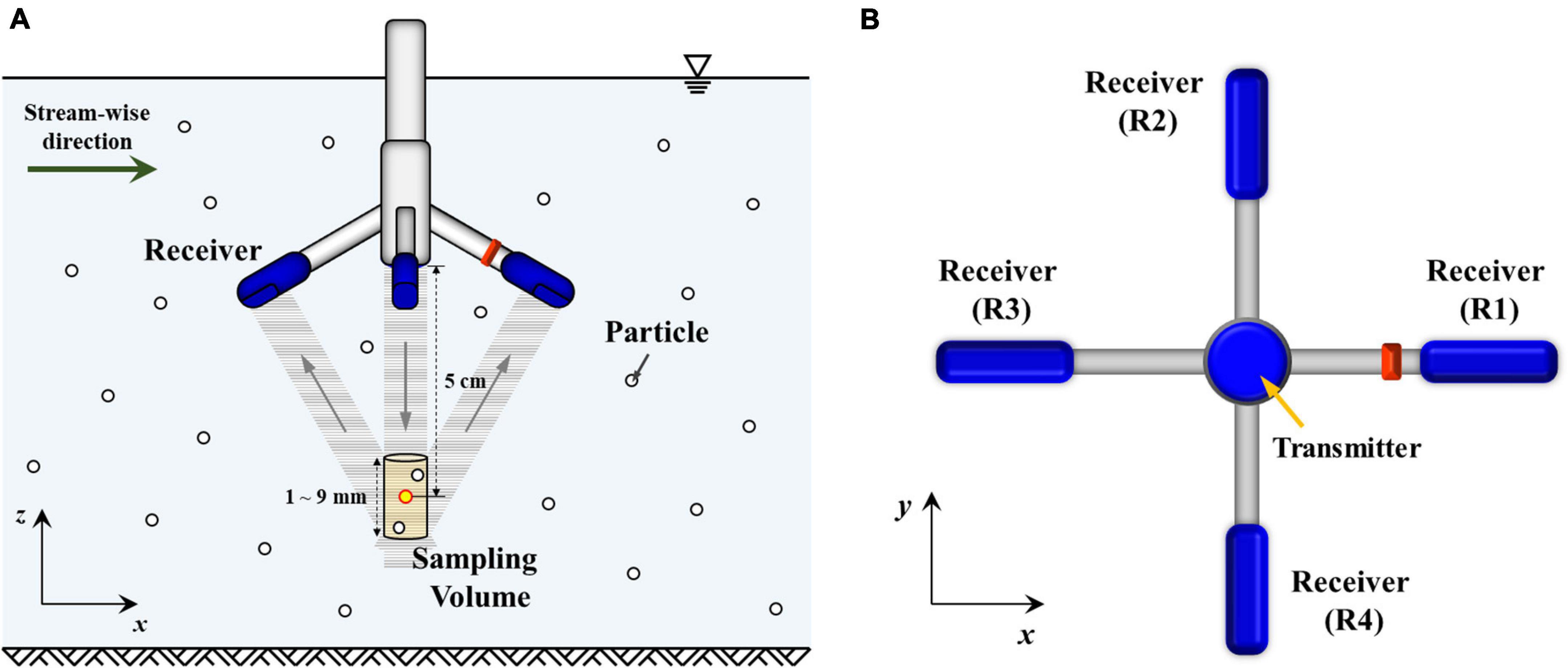
Figure 1. Schematic diagram of ADV system: (A) Side view; (B) top view.

where the subscript i can be from 1 to 4 and denotes the component in each receiver, c is the speed of sound in water, f_ADV is the frequency of sound emitted by the ADV device, and dϕ/dt is the phase difference given by

$$\frac{d\varphi }{dt}=\frac{1}{\mathrm{\Delta }t}{\tan }^{-1}\left[\frac{\sin \left[\varphi \left(t\right)\right]\cos \left[\varphi \left(t+\mathrm{\Delta }t\right)\right]-\sin \left[\varphi \left(t+\mathrm{\Delta }t\right)\right]\cos \left[\varphi \left(t\right)\right]}{\cos \left[\varphi \left(t\right)\right]\cos \left[\varphi \left(t+\mathrm{\Delta }t\right)\right]+\sin \left[\varphi \left(t\right)\right]\sin \left[\varphi \left(t+\mathrm{\Delta }t\right)\right]}\right],(2)$$

where ϕ is the signal phase in radians, t is the time, and Δt is the time difference between transmissions.

The ADV device (Vectrino+) used in this study is a point measurement instrument having a downward-looking probe with four receivers. In this four-receiver configuration, all receivers are orthogonal to each other and surrounding the transmitter. Two receivers deployed in the longitudinal direction (R1 and R3 in Figure 1B) measure the streamwise velocity, u and vertical velocity, w₁, whereas the remaining two receivers that are arranged in the transverse direction (R2 and R4 in Figure 1B) measure the transverse velocity, v, and vertical velocity, w₂. Here, the vertical velocities, w₁ and w₂, are measured redundantly but independently, and this arrangement can be utilized for noise analysis (Doroudian et al., 2010).

The radial flow velocity components along each receiver axis (V₁, V₂, V₃, and V₄) are obtained by the Eq. 1 and then transformed into the Cartesian coordinate system (u, v, w₁, and w₂) by multiplying the 4×4 transformation matrix T_m as follows:

$$\left[\begin{array}{c}\hfill u\hfill \\ \hfill v\hfill \\ \hfill w_1\hfill \\ \hfill w_2\hfill \end{array}\right]=\underset{T_m}{\underbrace{\left[\begin{array}{cccc}\hfill a_{11}\hfill & \hfill a_{12}\hfill & \hfill a_{13}\hfill & \hfill a_{14}\hfill \\ \hfill a_{21}\hfill & \hfill a_{22}\hfill & \hfill a_{23}\hfill & \hfill a_{24}\hfill \\ \hfill a_{31}\hfill & \hfill a_{32}\hfill & \hfill a_{33}\hfill & \hfill a_{34}\hfill \\ \hfill a_{41}\hfill & \hfill a_{42}\hfill & \hfill a_{43}\hfill & \hfill a_{44}\hfill \end{array}\right]}}\cdot \left[\begin{array}{c}\hfill V_1\hfill \\ \hfill V_2\hfill \\ \hfill V_3\hfill \\ \hfill V_4\hfill \end{array}\right],(3)$$

The transformation matrix elements are determined based on the geometric relationship between the transmitter and receivers during the calibration process by the manufacturer. Accordingly, each ADV device has its transformation matrix, as introduced in Table 1, which remains invariant unless the equipment undergoes physical deformation (Voulgaris and Trowbridge, 1998).

TABLE 1

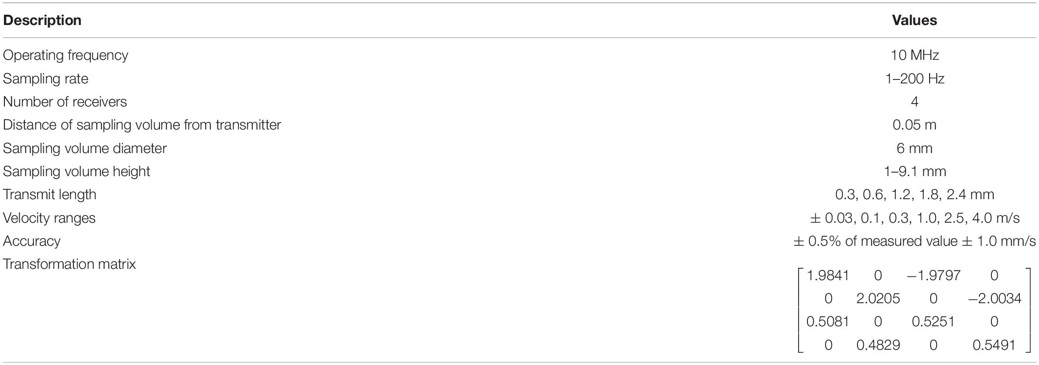
Table 1. Specification of ADV.

Experimental Setup

Two kinds of laboratory experiments were performed in the Hydraulic and Coastal Engineering Laboratory of Seoul National University. The first kind of experiment was conducted in still water to evaluate the system and surrounding noises of the ADV device in the various velocity ranges and sample volumes for setup. Still water conditions were created by filling water with seeding particles into a bucket, and the velocity was measured 12 cm away from the bottom when no movement was observed at the water surface. Data were collected in a total of 125 cases by changing five transmit length (0.3, 0.6, 1.2, 1.8, and 2.4 mm), five heights of sampling volume determined depending on the transmit length, and five nominal velocity ranges (± 0.03, 0.1, 0.3, 1.0, and 2.5 m/s). The velocity was measured at 100 Hz for 100 s in each case.

The second kind of experiments was performed in a 6.5-m-long, 0.15-m-wide, and 0.3-m-deep glass-walled recirculating flume to evaluate the proper sampling duration required to collect the various turbulence statistics. As presented in Table 2, the present work analyzed eight flow conditions with cross-sectional averaged streamwise velocities (U) ranging from 0.10 to 0.37 m/s. The vertical profile of the turbulent statistics was obtained from measurements taken at several locations over the acrylic bed for each flow condition. The data acquisition period lasted approximately 1 h for each measurement depth at 30 Hz to ensure that the data were sufficiently long to describe the turbulence field in the open channel as Chanson (2008) suggests. In the time series of the velocity data, the spikes that can overestimate the turbulence statistics were excluded and replaced following the phase-space threshold method suggested by Goring and Nikora (2002).

TABLE 2

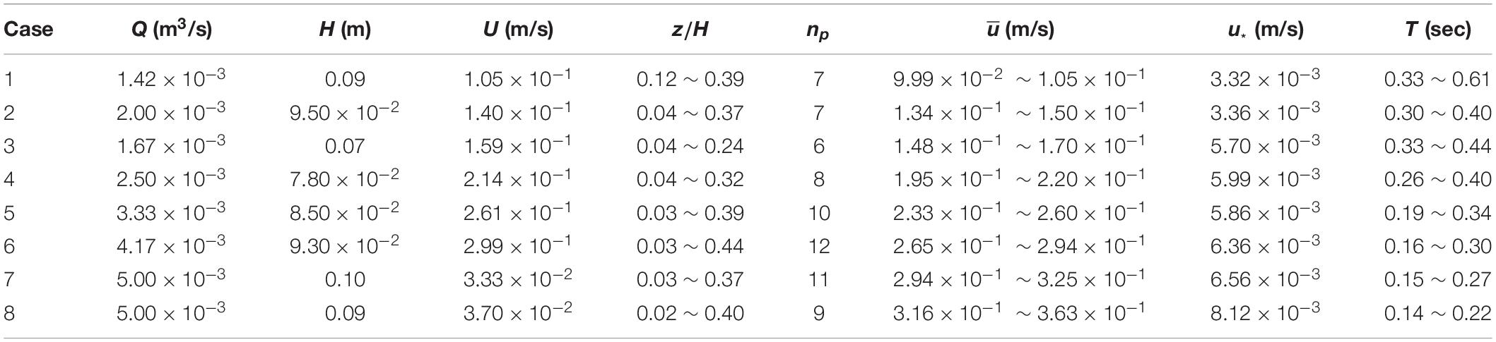
Table 2. Experimental conditions.

Determination of Record Length

When turbulence quantities are measured in a flow, the proper sampling duration needs to be selected carefully because a shorter sampling time loses the lower-frequency turbulent motions, whereas an excessive sampling time reduces the efficiency of the experimental procedures and does not allow to have the required spatial resolution. To determine the proper sampling duration, the non-parametric bootstrap sampling method and reverse arrangement test were applied in the present work. Supplementary Figure A.1 illustrates the overall procedures, and each process can be described as follows. The first step is to compute the integral time scale characterizing the time scale of the largest eddies from the measured velocities based on the following equation (Nystrom et al., 2007):

$$T_i\equiv {\int }_0^{t_0}{R}_i\left(\mathrm{\tau }\right)\mathit{d}\mathrm{\tau },(4)$$

where τ is a time lag between two points in time series data, t₀ is the time of the first zero-crossing in the normalized autocorrelation function (O’Neill et al., 2004). R_i(τ) can be calculated as follows:

$$R_i\left(\mathrm{\tau }\right)\equiv \frac{⟨u_i\left(t\right)u_i\left(t+\mathrm{\tau }\right)⟩}{⟨u_i{\left(t\right)}^2⟩},(5)$$

here, u_i(t) is the velocity component, and the subscript i denotes the x, y, or z direction. The integral time scale is calculated for each direction, and the maximum value among them becomes the representative integral time scale (T).

The next step is sampling data sequentially within the entire time series dataset based on the bootstrap sampling method. To elaborate, 1000 subsamples with a length of the integral time scale were extracted at a random location and five hydraulic parameters representing the flow characteristics such as the temporal-averaged stream-wise velocity ($\overline{u}$), the stream-wise and vertical turbulence intensities ($u_{\text{rms}}^{\prime }$ and $w_{\text{rms}}^{\prime }$), the Reynolds shear stress ($\overline{u^{\prime }{w}^{\prime }}$), and the turbulent kinetic energy (k) were computed for all subsamples. And then the standard error was calculated from the following equation:

$${\epsilon }_X=\sqrt{\frac{\sum _{m=0}^{m=N}{\left(X_m-⟨X⟩\right)}^2}{N-1}},(6)$$

where, ε_X is the standard error of the hydraulic parameter, N is the number of subsamples fixed as 1000 in this work, X is one of the five hydraulic parameters and ⟨X⟩ is the ensemble average of the selected parameter over 1000 subsamples. Once ε_X for the subsamples with a length of the integral time scale are computed, the next step is to repeat the above procedure by changing the length of subsample. The length of the subsample was determined as 1–1000 times of the integral time scale and the standard error of each case is represented by ε_α,X . Here, α ranging from 1 to 1000 means the length of the subsample. As an example, ε_1,X and ε_1000,X are the standard errors of subsample having a length of 1 and 1000 times the integral time scale, respectively.

When we set X equal to $u_{\text{rms}}^{\prime }$, the variation of the standard error for $u_{\text{rms}}^{\prime }$ with α can be represented in Figure 2. According to Figure 2, the slope of the standard error (${\mathrm{\epsilon }}_X^{\prime }$ (= dε_X/dα)) approaches zero with increasing α and eventually converges. This means that when the sample length exceeds a critical value, the hydraulic parameter changes no longer. To define the starting point of convergence (α_c), the reverse arrangement test allowing us to quantify whether a significant trend in the dataset (Beck et al., 2006) was applied to ${\mathrm{\epsilon }}_X^{\prime }$ . Firstly, a sequence of n observations of ${\mathrm{\epsilon }}_X^{\prime }$ was extracted, where the observations are denoted as ${\mathrm{\epsilon }}_{p,X}^{\prime }$ and p is from α to α+n-1 (e.g., α = 1, n = 3: observations = ${\mathrm{\epsilon }}_{1,X}^{\prime }$, ${\mathrm{\epsilon }}_{2,X}^{\prime }$, ${\mathrm{\epsilon }}_{3,X}^{\prime }$). In the present study, n was determined to be 100, which is long enough to represent the overall trend of the dataset. The second step was counting the number of times that ${\mathrm{\epsilon }}_{p,X}^{\prime }>{\mathrm{\epsilon }}_{q,X}^{\prime }$ for p < q and to compute A based on the following equation:

FIGURE 2

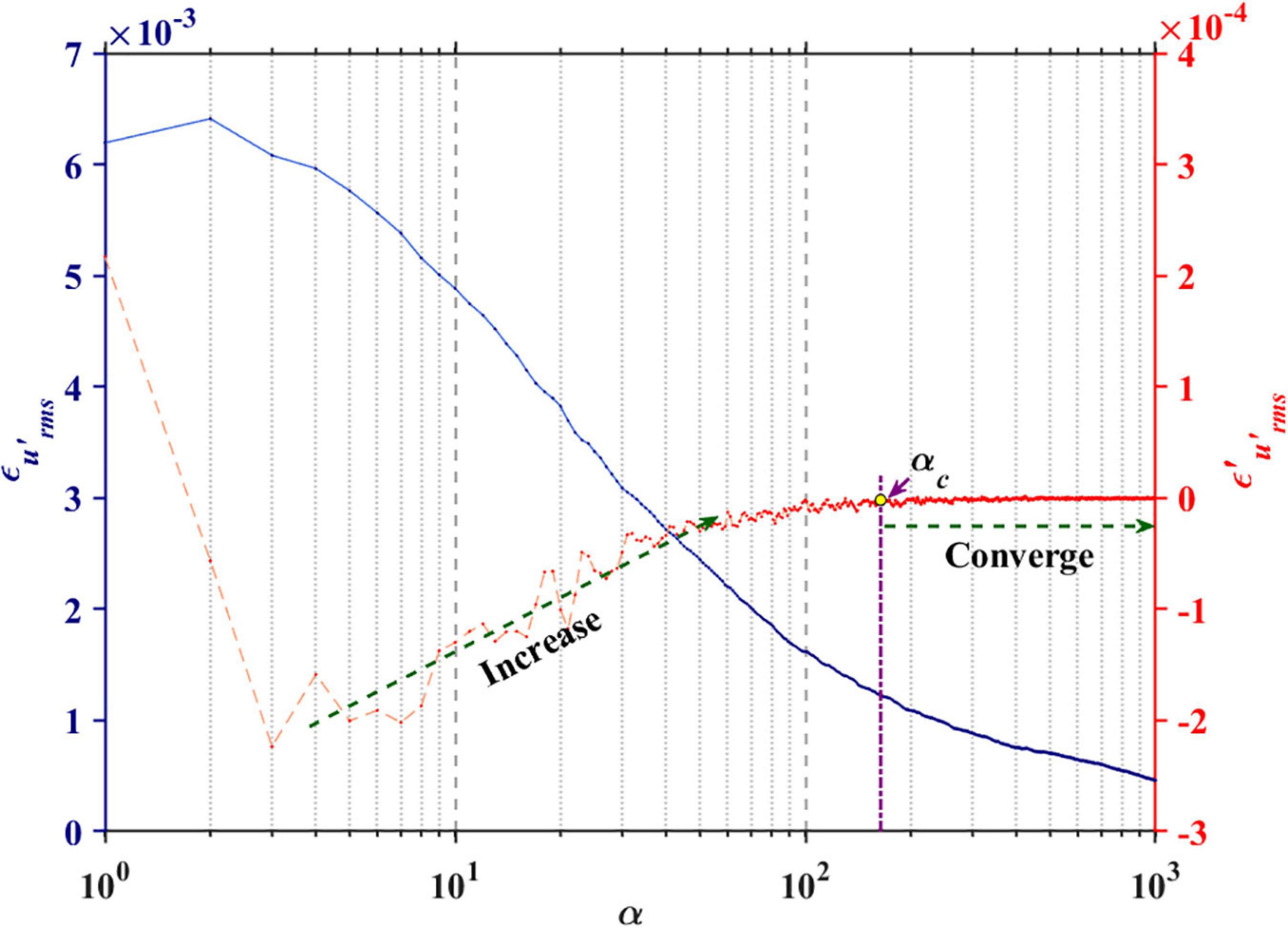
Figure 2. Variation of ${\mathrm{\epsilon }}_{u_{\text{rms}}^{\prime }}$ and ${\mathrm{\epsilon }}_{u_{\text{rms}}^{\prime }}^{\prime }$ with the sample length, α.

$$A=\sum _{p=1}^{n-1}\sum _{q=p+1}^n{h}_{pq},(7)$$

where

$$h_{pq}=\{\begin{array}{cc}\hfill 1\hfill & \hfill \text{if}{\mathrm{\epsilon }}_{p,X}^{\prime }>{\mathrm{\epsilon }}_{q,X}^{\prime }\hfill \\ \hfill 0\hfill & \hfill \text{otherwise}\hfill \end{array},(8)$$

The third step is evaluating a z-score by using the following equation and performing a hypothesis test with a significance level of 0.05:

$$z=\frac{A-\left[\frac{n\left(n-1\right)}{4}\right]}{\sqrt{\frac{2n^3+3n^2-5n}{72}}},(9)$$

Our null hypothesis was that there is no trend in the sequence of extracted ${\mathrm{\epsilon }}_{p,X}^{\prime }$, whereas the alternative hypothesis is that there is an increasing or decreasing trend. We repeated the above procedures by increasing α and when α failed to reject the null hypothesis, this value becomes α_c. The details and examples of the reverse arrangement test are provided in Bendat and Piersol (2011).

Results and Discussion

Still Water Experiment

In still water, all velocity fields should be zero, and so measured residuals of signals represent the noises due to instrumental system and surroundings. Figure 3 shows the relationships between the height of sampling volume (H_s) and the variances of fluctuating signals (${\mathrm{\sigma }}_n^2$) from each receiver in the various settings of velocity range (V_R). Here, ${\mathrm{\sigma }}_n^2$ can be regarded as the magnitude of noises in the normal direction to the transmitter. Figure 3A shows that the noises decrease with increasing H_s in all velocity ranges for setup, since a larger sampling volume has more numbers of suspended particle and this intensifies backscattering signals and attenuates the noises. In a fixed sampling volume, the noises increase as the velocity range for setup increases, similar to the results obtained in previous studies (Nikora and Goring, 1998; Voulgaris and Trowbridge, 1998), in which experiments identical to the present cases were performed, but with three-receiver ADV.

FIGURE 3

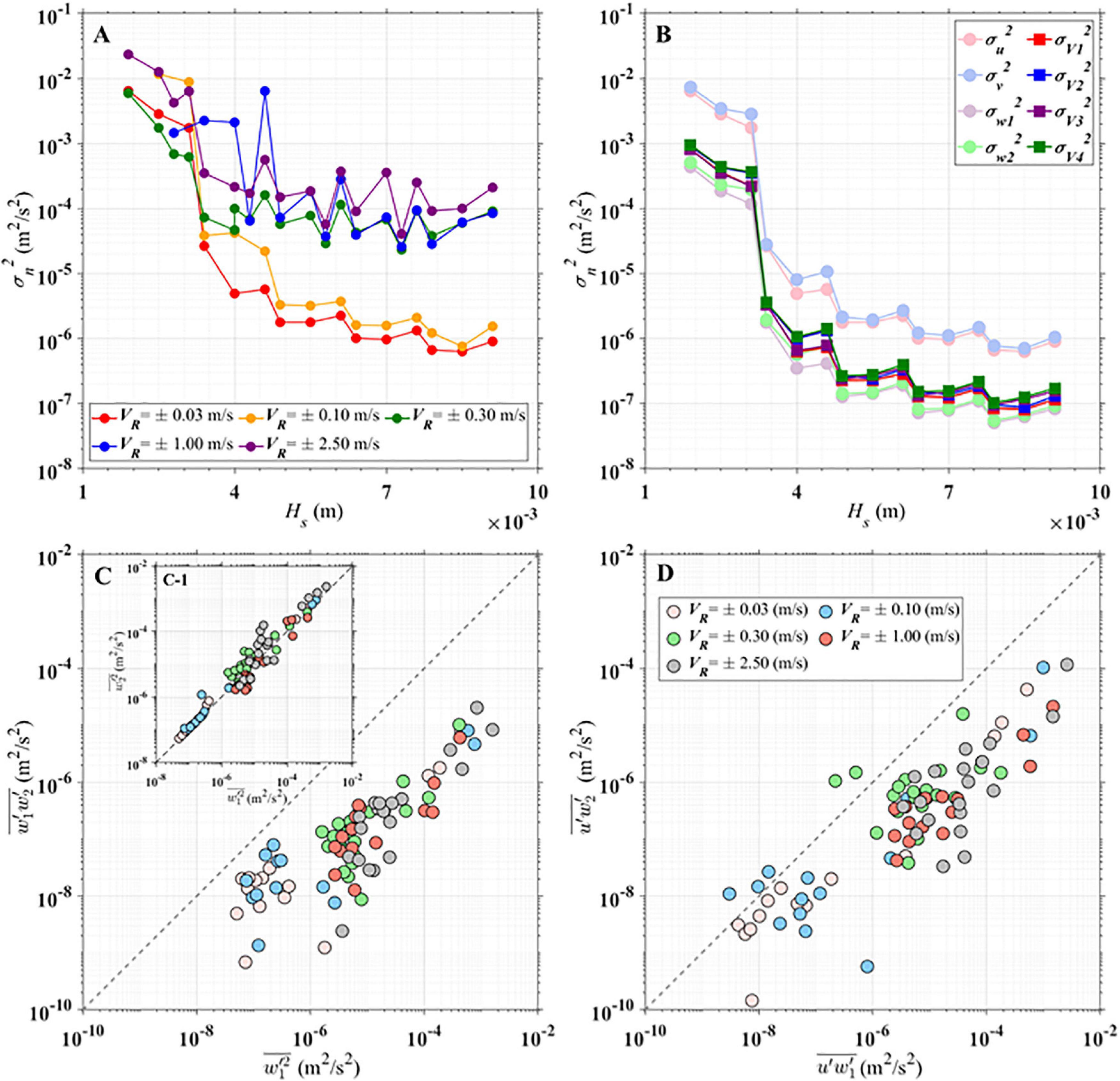
Figure 3. (A) Relation between the noise variance of stream-wise velocity component and the height of sampling volume in the different velocity ranges for setup. (B) The relation between the noise and the height of sampling volume for V_R = ±0.03 m/s. Relationship between (C) $\overline{w_1^{\prime }{}^2}$ and $\overline{w_1^{\prime }{w}_2^{\prime }}$ and between (D) $\overline{u^{\prime }{w}_1^{\prime }}$ and $\overline{u^{\prime }{w}_2^{\prime }}$ in different velocity ranges: the dotted lines mean that y = x.

Figure 3B presents the variances of the fluctuating signals collected from each receiver in the velocity range of ±0.03 m/s for setup. The paled colored lines indicate the noise variance of each velocity component in the Cartesian coordinate system (${\mathrm{\sigma }}_u^2$, ${\mathrm{\sigma }}_v^2$, ${\mathrm{\sigma }}_{\mathrm{w1}}^2$, and ${\mathrm{\sigma }}_{\mathrm{w2}}^2$), and the dark colored lines indicate the noises of the velocity component along each receiver axis (${\mathrm{\sigma }}_{\mathrm{V1}}^2$, ${\mathrm{\sigma }}_{\mathrm{V2}}^2$, ${\mathrm{\sigma }}_{\mathrm{V3}}^2$, and ${\mathrm{\sigma }}_{\mathrm{V4}}^2$). The noises of each receiver were calculated with Eq. 3 (e.g., ${\mathrm{\sigma }}_{\mathrm{V1}}^2$ =σ${}_u{}^2/(a_{11}^2+a_{13}^2)$). As shown in Figure 3B, the noises along the receiver axis are almost same to each other regardless of H_s, although they were significantly amplified or attenuated during the coordinate transformation to the real velocity field. Considering Table 1, the elements of the transformation matrix increase the noises of each receiver by 7.86$=a_{11}^2+a_{13}^2$, 8.10$=a_{22}^2+a_{24}^2$, 0.53$=a_{31}^2+a_{33}^2$, and 0.54$=a_{42}^2+a_{44}^2$ for the u, v, w₁, and w₂ velocity components, respectively. As a result, the horizontal noises included in the streamwise and transverse normal stresses ($\overline{u^{\prime 2}}$ and $\overline{v^{\prime 2}}$) are approximately 15 times higher than the vertical ones included in the vertical normal stresses ($\overline{w_1^{\prime }{}^2}$ and $\overline{w_2^{\prime }{}^2}$). This tendency is analogous to that observed by Nikora and Goring (1998), who concluded that the horizontal velocity components include a significantly higher level of noise than the vertical component owing to the geometry of the three-receiver ADV system.

Although the noises in the measuring procedure cannot be eliminated, the noises in the vertical component can be reduced by using two vertical velocities measured with the orthogonally deployed receivers. In the present ADV, there are several ways to determine the variances of the vertical velocities. Two vertical velocities can be measured and compute the vertical normal stresses, $\overline{w_1^{\prime }{}^2}$ and $\overline{w_2^{\prime }{}^2}$ and another way is to use both two vertical velocities simultaneously measured from the orthogonally deployed receivers and compute $\overline{w_1^{\prime }{w}_2^{\prime }}$. Figure 3C compares the magnitudes of noise in the vertical normal stresses estimated using these methods. In all velocity ranges for setup, $\overline{w_1^{\prime }{}^2}$ and $\overline{w_2^{\prime }{}^2}$ have a strong linear correlation with each other (Figure 3C-1), indicating that they contain similar magnitudes of noise. In contrast, $\overline{w_1^{\prime }{w}_2^{\prime }}$ is O(10^–1–10^–2) times less than $\overline{w_1^{\prime }{}^2}$ because the random noises from the orthogonally deployed receivers are statistically and theoretically uncorrelated, which leads to a noise covariance close to zero (Blanckaert and Lemmin, 2006).

Such a trend can also be found in Figure 3D, which presents the noise of the turbulent shear stresses estimated from the same pair of receivers ($\overline{u^{\prime }{w}_1^{\prime }}$) and orthogonally deployed receivers ($\overline{u^{\prime }{w}_2^{\prime }}$). The results for $\overline{u^{\prime }{w}_2^{\prime }}$ are generally less than those for $\overline{u^{\prime }{w}_1^{\prime }}$, which also supports the argument that the orthogonality in the deployment of receivers helps to reduce the noise when turbulent stress is estimated. Besides, the correlation coefficients u’ and $w_1^{\prime }$ and between u’ and $w_2^{\prime }$ were computed to be 0.25 and 0.01, respectively. These findings indicate that the noise signals measured from orthogonally positioned receivers are independent of each other and thus would be canceled out during the turbulent shear stress calculation process.

In addition to the system noises, when the flow velocity exceeds instantaneously the measurable range of the instrument or when an obstacle blocks the sound path between the transmitter and receiver, spurious spiking signals occur, and they constitute one of the main sources of error influencing the turbulent stresses (Doroudian et al., 2010). Interestingly, in the case of the four-receiver ADV system, spikes are detected simultaneously in the same pair of receivers (Supplementary Figure A.2), leading to significant overestimation of the turbulent stresses. However, utilizing the velocities measured from the orthogonally positioned receivers enables this error to be corrected, yielding a relatively error-free turbulent stress.

Experiments in Channel Flows

In open channel flows, the sampling period or time may be strongly influenced by the flow characteristics and the measurement conditions. Before determining the optimal sampling time, we computed several hydrodynamic parameters representing the turbulent characteristics of flows. A total of six parameters, namely, the temporally averaged streamwise velocity ($\overline{u}$), streamwise turbulent intensity ($u_{\text{RMS}}^{\prime }$), Reynolds shear stress ($\overline{u^{\prime }{w}^{\prime }}$), integral time scale (T), integral length scale (L), and shear velocity (^u*) were considered. Here, $u_{\text{RMS}}^{\prime }$ was computed as $\sqrt{\overline{u^{\prime 2}}}$ and the Reynolds shear stress ($\overline{u^{\prime }{w}^{\prime }}$) is calculated as $\overline{u^{\prime }{w}_2^{\prime }}$ based on the result of still water experiment. The overbar denotes the temporal average, and the prime indicates the velocity fluctuations computed by subtracting the temporally averaged velocity from the instantaneous velocities, e.g., $u^{\prime }=u-\overline{u}$. The integral time scale was calculated from Eq. 4 and the integral length scale was determined by multiplying the temporal-averaged velocity ($\overline{u}$) times the integral time scale at each measurement point ($L=\overline{u}\cdot T$).

The shear velocity was computed with the law of the wall applicable to a near-wall region of the turbulent boundary layer (Nezu and Rodi, 1986):

$$u^{+}=\frac{1}{\mathrm{\kappa }}\ln \left(z^{+}\right)+C,(10)$$

where κ is the von Karman constant (≈0.41); u⁺ and z⁺ are defined as $\overline{u}/u_{*}$ and zu_*/ν , respectively; z is the distance of the measurement point from the bottom; v is the kinematic viscosity of water; and C is a constant. Rearranging Eq. 10, the relationship between ln (z) and $\overline{u}$ becomes linear as follows:

$$\overline{u}=\frac{u_{*}}{\mathrm{\kappa }}\ln \left(z\right)+\frac{u_{*}}{\mathrm{\kappa }}\ln \left(\frac{u_{*}}{\mathrm{\nu }}\right)+u_{*}C,(11)$$

Because the above equation is applicable only to the logarithmic layer within the boundary layer, the measurement data satisfying the linear relationship were selected in this study and the shear velocity was computed from the slope of the trend line (solid line in Figure 4A) of the selected data.

FIGURE 4

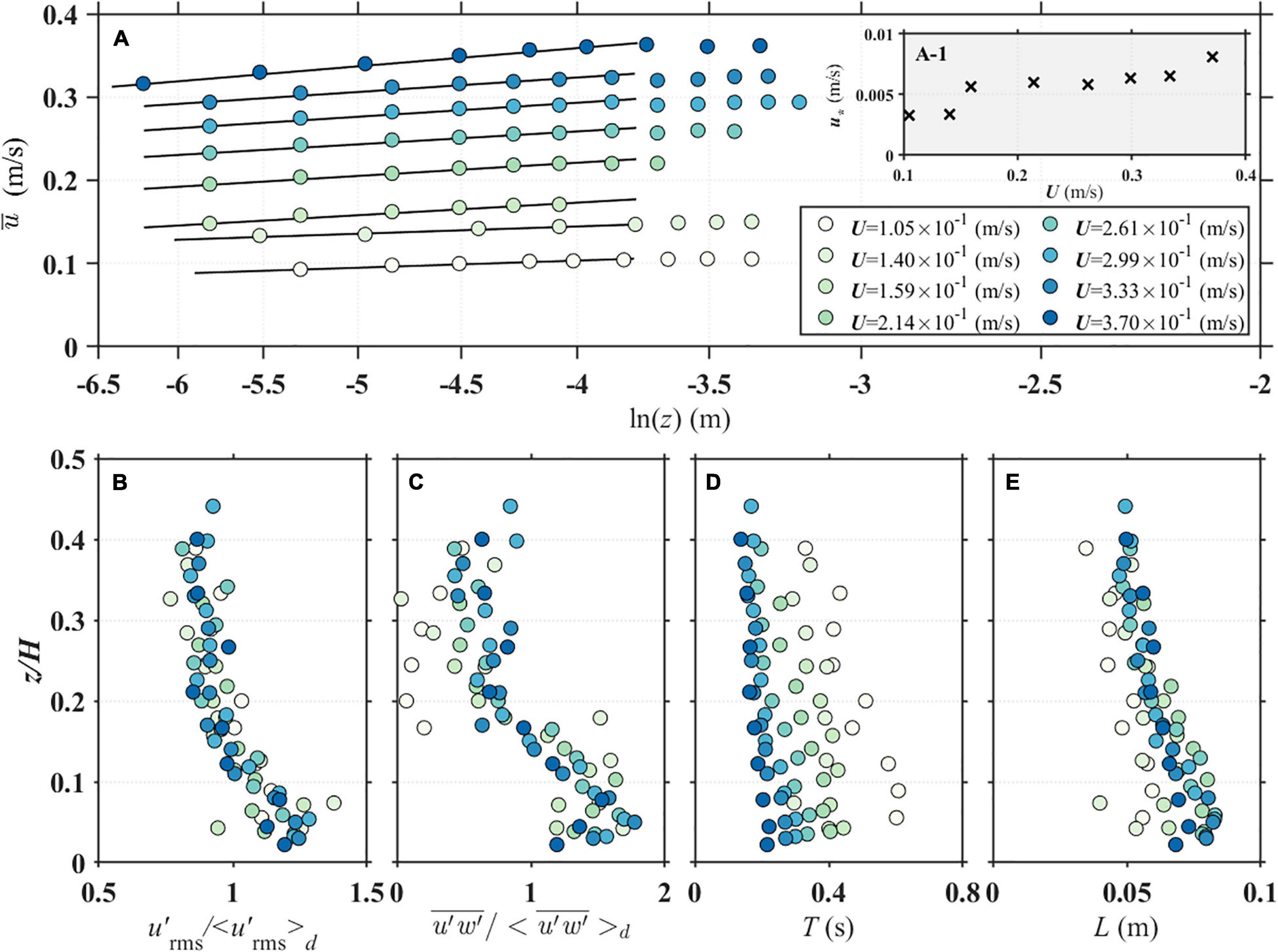
Figure 4. Vertical profiles of the (A) temporal averaged stream-wise velocity, (B) stream-wise turbulence intensity, (C) Reynolds shear stress, (D) integral time scale, and (E) integral length scale.

According to Figure 4A, the shear velocity (u_*) increases linearly from 0.003 to 0.008 m/s as the inlet flow velocity (U) increases and this trend is similar to that obtained by Carvalho et al. (2010), who measured the shear velocity over the Perspex plate under flow conditions similar to those considered in this study. Figures 4B,C present the vertical distributions of the non-dimensional streamwise turbulence intensity ($u_{\text{RMS}}^{\prime }$) and the Reynolds shear stress ($\overline{u^{\prime }{w}^{\prime }}$), respectively. Those parameters are non-dimensionalized with the depth-averaged values, ${⟨u_{\text{RMS}}^{\prime }⟩}_d$ and ${⟨\overline{u^{\prime }{w}^{\prime }}⟩}_d$, respectively. In all flow conditions, the turbulent intensity and Reynolds shear stress increase toward the bed and both reach maxima at z/H ≈ 0.05. Near the bed region (z/H < 0.05), the viscous effect dominates the turbulent fluctuations, decreasing the turbulence quantities as expected.

Figures 4D,E, respectively, depict the computed integral time (T) and length (L) scales and their vertical profiles. The integral time scale increases with the decrease of U at the same locations. In the same flow conditions, differently from the length scale, the length scale is spatially larger in the near bed, where the mean flow is relatively slower than that in the outer region, as similarly observed by Köse (2011). In most of the experiments, integral length scales range from 0.04 to 0.08 m and the scales increase toward the bed since the bottom friction generates a strong shear near the bottom boundary layer than in the upper region and this shear produces larger turbulent eddies. Much closer to the bottom (z/H < 0.05), the integral length scale decreases, similar to the turbulent intensity and Reynolds shear stress, because the viscous effect suppresses the formation of turbulent eddies. While the integral time scale varies with the flow condition (Figure 4D), the integral length scales are almost similar to each other in each depth of all flow conditions (Figure 4E) since they are constructed with the integral time scale and the mean velocity which seems to be very close to time scale and velocity scale of the largest eddies.

Figure 5 shows the optimal sampling period for the turbulence statistics determined by using the reverse arrangement test. Considering the results from the still water experiments, the vertical turbulent intensity ($w_{\text{rms}}^{\prime }$) and the turbulent kinetic energy (k) were computed as $\sqrt{\overline{w_1^{\prime }{w}_2^{\prime }}}$ and $\left(\overline{u^{\prime 2}}+\overline{v^{\prime 2}}+\overline{w_1^{\prime }{w}_2^{\prime }}\right)/2$, respectively. According to Figure 5A, the optimal sampling period ranges between 150 and 200 times the integral time scale for all turbulence statistics, indicating that for the turbulence statistics to reach a stationary state, at least 150 numbers or more of the integral scales of the largest eddies should be included during the measurement period. If we convert those critical number α_c into a recognizable real-time length by multiplying it times the integral time scale at each measurement as T_c = α_c.T, the optimal sampling duration falls in the range of 40–60 s for all turbulence statistics (Figure 5B), which is similar to Buffin-Bélanger and Roy (2005).

FIGURE 5

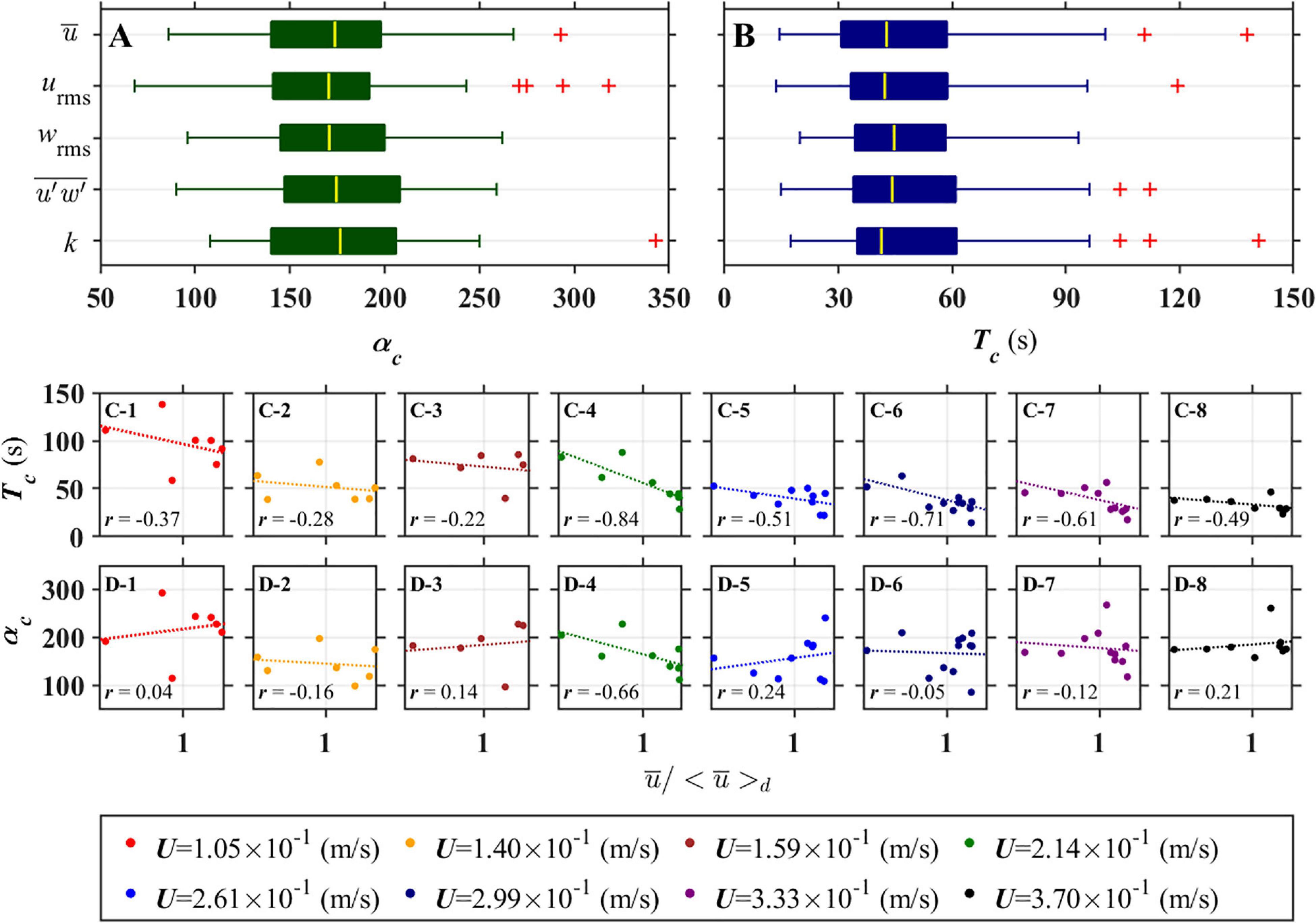
Figure 5. Optimal sampling time of hydraulic parameters represented by (A) α_c and (B) real-time scale (T_c). The red plus signs indicate outliers. The relation between the non-dimensional stream-wise velocity and (C) T_c, and (D) α_c: r is the correlation coefficient.

Figures 5C,D present the variations of the optimal sampling period with the changes of the mean velocity when the sampling period is determined with the real-time duration (T_c) and the multiple of integral time scale (α_c). As shown in Figure 5C, T_c decreases with increasing U, which indicates that a longer sampling time is not required for the faster flows since it takes less time to capture turbulent eddies than in the slower flows if the sizes of the eddies are same in both flows. Such inverse relations can also be found in each flow condition, where the average correlation coefficient between $\overline{u}$ and T_c is evaluated to be approximately −0.51. At a fixed inlet velocity, a longer measurement time is required for a near-wall region since flow is much slower but turbulent eddy is larger than the upper region (Figure 4E). This finally causes a negative correlation coefficient between $\overline{u}$ and T_c.

Contrary to T_c, α_c is independent and uncorrelated with flow characteristics, thus, there is no specific trend (Figure 5D) and so the average correlation coefficients between α_c and mean velocities are around –0.05. In other words, the sampling period based on α_c is more independent of the flow characteristics and conditions than that based on T_c. This result can also be found clearly in Supplementary Figure A.3, which shows the relationship between $\overline{u}$ and T_c, and α_c for all cases. In this regard, when we establish a criterion for the optimal sampling period, it is more appropriate to use multiple of integral time scales as the basic unit rather than using real-time, which has high variability depending on the flow conditions.

To verify that the proposed optimal sampling period is long enough to describe the physical characteristics of turbulent flow, we spectrally analyzed the assumed true value (velocity data measured for approximately 1 h) and the data sampled during the optimal sampling period. The assumed true values were separated into several sets by dividing by a proposed optimal sampling time and the spectral densities of each set are were constructed and then those spectra were ensemble-averaged for presenting smooth spectral functions.

Figures 6A,B present the power spectral densities of streamwise and vertical turbulence intensities, respectively. The red and black lines represent the spectra of the assumed true values and optimal sampling period, respectively. Although the variance of the spectrum for data with an optimal sampling period is much larger than that of the assumed true value, they follow a similar trend. In the case of stream-wise velocity (Figure 6A), the inertial subrange having a –5/3 slope of power is hardly detected in either spectrum, and they become white noises in the range with higher frequencies owing to the instrumental or system limitations. In the case of vertical velocity (Figure 6B), the spectra follow a –5/3 slope well from 4 Hz to the Nyquist frequency without a white noise spectrum. Such results indicate that the streamwise velocity contains more noises than the vertical velocity, as discussed in the results of the still water experiment related to the elements of the transformation matrix, which amplify the noise variances by a factor of 15 in the streamwise velocity compared to the vertical velocity.

FIGURE 6

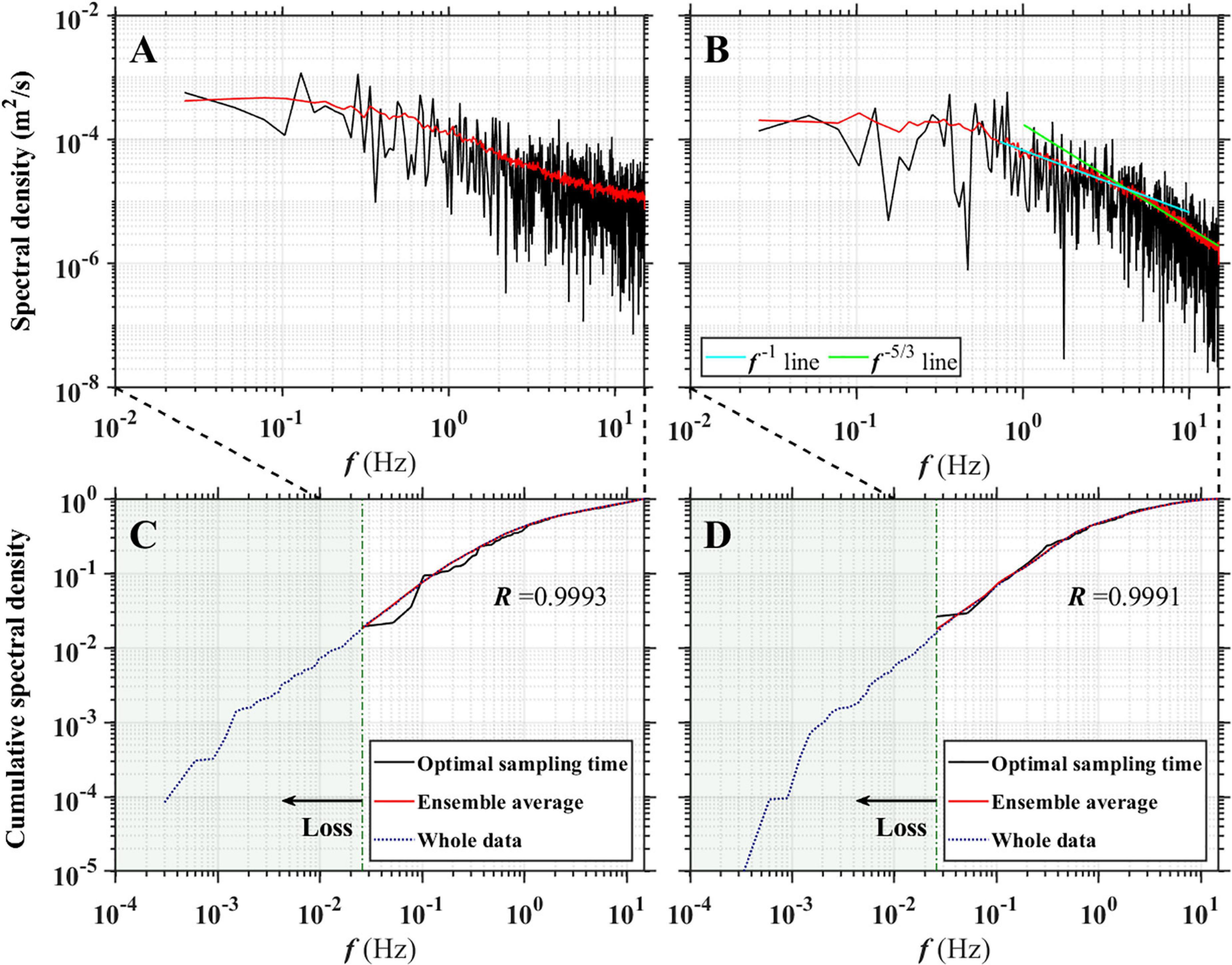
Figure 6. Power spectral densities of (A) u’ and (B) w’ and cumulative spectral densities of (C) u’ and (D) w’; The black line means the spectrum of a randomly chosen data having a length of optimal sampling time and the maximum frequency of power spectral densities is half of the sampling frequency.

Figures 6C,D depict the cumulative power spectra. The y axis represents the ratio of the energy of motion with a frequency less than f to the whole energy. When the spectrum is obtained from data with an optimal sampling period, a shorter sampling period limits the length or period of the flow motion that can be captured, and thus, the spectral density starts from 0.02 Hz. In the frequency range of 0.02 < f < 0.1 Hz, the energies occupy about 10% of the entire turbulence energy and the assumed true values and data having optimal sampling time show less than 2% disparity with each other, whereas they become identical at higher frequencies (f > 0.1 Hz), which is responsible for the remaining 90% of energy. Besides, the correlation coefficient between them for u’ and w’ is larger than 0.99, indicating that the data collected during the optimal sampling period are sufficient to describe the flow characteristics of the assumed true values.

Because it is impossible to capture flow motions with frequencies less than 0.02 Hz for the optimal sampling period, the corresponding flow motions and energies are lost. To investigate the amount of energy lost due to sampling time truncation, we also calculated the cumulative spectral density of the entire velocity data without an ensemble average (navy dotted lines in Figures 6C,D). According to the green-colored areas in Figures 6C,D, the energy losses at low frequencies are negligibly small as 1.6 and 1.1% for u’ and w’, respectively, signifying that there is little energy loss due to the sampling time truncation.

Conclusion

The present work proposed an appropriate operating method for a four-receiver ADV that can yield reliable turbulence quantities. Laboratory experiments were performed using this instrument and the proposed method under two flow conditions, and the principal findings of each experiment can be summarized as follows.

(a) The orthogonality in the deployment of four-receivers of the ADV has a great advantage in measuring the shear stresses. Transforming the received signals to the coordinates for each velocity modifies the electrical noises of the signals. Before transforming the signals to the velocity component, this original signals at each receiver are in a similar range of electrical noises, but after the signals were transformed to the velocity directions, the noise variances are amplified by approximately eight times in the stream-wise and lateral directions and they are reduced by half in the vertical direction. However, the Reynolds stresses were computed with the velocities obtained by the orthogonally deployed receivers and this orthogonality erases the uncorrelated random noises from each receiver in the Reynolds stress calculation.

(b) The integral time scale of turbulence is proposed as a base for an optimal sampling period. 150–200 times of the integral time scale seems to be almost invariant regardless of the measurement conditions. The conventionally proposed method based on a fixed real scale sampling period (e.g., 1,000 s) asks the various sampling periods depending on the vertical and horizontal locations even in a flow. For example, a near-wall region, where the mean flow velocity is relatively low and turbulent eddies are larger than other areas, requires a longer measurement time compared to a region far from the wall, where the mean flow is much higher and turbulent eddies are relatively small. In this regard, the integral time scale which reflects the information of the size of large eddies is a more suitable base than real-time scales for a sampling time criterion.

Although our approaches help to overcome the ambiguities faced by the previous researches using ADV, several limitations still remain with requiring future work. For example, since our framework was established through laboratory experiments with the assumption of stationary flow, it should be extended to the non-stationary flows with various scales of turbulent motion and also studied more for the application to the field experiments. Nevertheless, we expect that our framework will enable researchers to measure the Reynolds stress and other turbulence quantities effectively and obtain reliable data for fluid dynamics analysis.

Data Availability Statement

The original contributions presented in the study are included in the article/Supplementary Material, further inquiries can be directed to the corresponding author.

Author Contributions

HP performed laboratory experiments, analyzed the results, and wrote the original manuscript. JH conceptualized this research, reviewed the manuscript, and focused on revising the section “Results and Discussion.” Overall, both authors contributed significantly and shared a lot of work and approved the submitted version.

Funding

This research was supported by Basic Science Research Program through the National Research Foundation of Korea (NRF) funded by the Korean Government Ministry of Science, ICT and Future Planning (No. 2020R1A2B5B01002249), Korean Ministry of Environment (MOE) as “Chemical Accident Response R&D program” (No. ARG201901179001), and administratively supported by the Institute of Engineering Research at Seoul National University.

Conflict of Interest

The authors declare that the research was conducted in the absence of any commercial or financial relationships that could be construed as a potential conflict of interest.

Publisher’s Note

All claims expressed in this article are solely those of the authors and do not necessarily represent those of their affiliated organizations, or those of the publisher, the editors and the reviewers. Any product that may be evaluated in this article, or claim that may be made by its manufacturer, is not guaranteed or endorsed by the publisher.

Supplementary Material

The Supplementary Material for this article can be found online at: https://www.frontiersin.org/articles/10.3389/fmars.2021.681265/full#supplementary-material

References

Beck, T. W., Housh, T. J., Weir, J. P., Cramer, J. T., Vardaxis, V., Johnson, G. O., et al. (2006). An examination of the runs test, reverse arrangements test, and modified reverse arrangements test for assessing surface EMG signal stationarity. J. Neurosci. Methods 156, 242–248. doi: 10.1016/j.jneumeth.2006.03.011

PubMed Abstract | CrossRef Full Text | Google Scholar

Bendat, J. S., and Piersol, A. G. (2011). Random Data: Analysis and Measurement Procedures, Vol. 729. Hoboken, NJ: John Wiley & Sons.

Google Scholar

Blanckaert, K., and Lemmin, U. (2006). Means of noise reduction in acoustic turbulence measurements. J. Hydraulic Res. 44, 3–17. doi: 10.1080/00221686.2006.9521657

CrossRef Full Text | Google Scholar

Buffin-Bélanger, T., and Roy, A. G. (2005). 1 min in the life of a river: selecting the optimal record length for the measurement of turbulence in fluvial boundary layers. Geomorphology 68, 77–94. doi: 10.1016/j.geomorph.2004.09.032

CrossRef Full Text | Google Scholar

Carvalho, E., Maia, R., and Proença, M. F. (2010). Shear stress measurements over smooth and rough channel beds. River Flow 2010, 367–376.

Google Scholar

Chanson, H. (2008). “Acoustic Doppler velocimetry (ADV) in the field and in laboratory: practical experiences,” in Proceeding of International Meeting on Measurements and Hydraulics of Sewers IMMHS’08, Summer School GEMCEA/LCPC, 19–21 August 2008, (Bouguenais).

Google Scholar

Chanson, H., Trevethan, M., and Koch, C. (2007). Discussion of “turbulence measurements with acoustic doppler velocimeters” by Carlos M. García, Mariano I. Cantero, Yarko Niño, and Marcelo H. García. J. Hydraulic Eng. 133, 1283–1286.

Google Scholar

Doroudian, B., Bagherimiyab, F., and Lemmin, U. (2010). Improving the accuracy of four-receiver acoustic Doppler velocimeter (ADV) measurements in turbulent boundary layer flows. Limnol. Oceanogr.: Methods 8, 575–591. doi: 10.4319/lom.2010.8.0575

CrossRef Full Text | Google Scholar

Goring, D. G., and Nikora, V. I. (2002). Despiking acoustic Doppler velocimeter data. J. Hydraulic Eng. 128, 117–126. doi: 10.1061/(asce)0733-9429(2002)128:1(117)

CrossRef Full Text | Google Scholar

Kim, S. C., Friedrichs, C. T., Maa, J. Y., and Wright, L. D. (2000). Estimating bottom stress in tidal boundary layer from acoustic Doppler velocimeter data. J. Hydraulic Eng. 126, 399–406. doi: 10.1061/(asce)0733-9429(2000)126:6(399)

CrossRef Full Text | Google Scholar

Köse, Ö (2011). Distribution of turbulence statistics in open-channel flow. Int. J. Phys. Sci. 6, 3426–3436.

Google Scholar

Lane, S. N., Biron, P. M., Bradbrook, K. F., Butler, J. B., Chandler, J. H., Crowell, M. D., et al. (1998). Three-dimensional measurement of river channel flow processes using acoustic Doppler velocimetry. Earth Surface Processes Landforms: J. British Geomorphol. Group 23, 1247–1267. doi: 10.1002/(sici)1096-9837(199812)23:13<1247::aid-esp930>3.0.co;2-d

CrossRef Full Text | Google Scholar

Lesht, B. M. (1980). Benthic boundary-layer velocity profiles: dependence on averaging period. J. Phys. Oceanogr. 10, 985–991. doi: 10.1175/1520-0485(1980)010<0985:bblvpd>2.0.co;2

CrossRef Full Text | Google Scholar

McLelland, S. J., and Nicholas, A. P. (2000). A new method for evaluating errors in high-frequency ADV measurements. Hydrol. Processes 14, 351–366. doi: 10.1002/(sici)1099-1085(20000215)14:2<351::aid-hyp963>3.0.co;2-k

CrossRef Full Text | Google Scholar

Nezu, I., and Rodi, W. (1986). Open-channel flow measurements with a laser Doppler anemometer. J. Hydraulic Eng. 112, 335–355. doi: 10.1061/(asce)0733-9429(1986)112:5(335)

CrossRef Full Text | Google Scholar

Nikora, V. I., and Goring, D. G. (1998). ADV measurements of turbulence: can we improve their interpretation? J. Hydraulic Eng. 124, 630–634. doi: 10.1061/(asce)0733-9429(1998)124:6(630)

CrossRef Full Text | Google Scholar

Nystrom, E. A., Rehmann, C. R., and Oberg, K. A. (2007). Evaluation of mean velocity and turbulence measurements with ADCPs. J. Hydraulic Eng. 133, 1310–1318. doi: 10.1061/(asce)0733-9429(2007)133:12(1310)

CrossRef Full Text | Google Scholar

O’Neill, P. L., Nicolaides, D., Honnery, D., and Soria, J. (2004). “Autocorrelation functions and the determination of integral length with reference to experimental and numerical data,” in Proceeding of the 15th Australasian Fluid Mechanics Conference, Vol. 1, (Sydney: University of Sydney), 1–4.

Google Scholar

Park, H., and Hwang, J. H. (2019). Quantification of vegetation arrangement and its effects on longitudinal dispersion in a channel. Water Resour. Res. 55, 4488–4498. doi: 10.1029/2019wr024807

CrossRef Full Text | Google Scholar

Petrie, J., Diplas, P., Gutierrez, M., and Nam, S. (2013). Data evaluation for acoustic Doppler current profiler measurements obtained at fixed locations in a natural river. Water Resour. Res. 49, 1003–1016. doi: 10.1002/wrcr.20112

CrossRef Full Text | Google Scholar

Reidenbach, M. A., Monismith, S. G., Koseff, J. R., Yahel, G., and Genin, A. (2006). Boundary layer turbulence and flow structure over a fringing coral reef. Limnol. Oceanogr. 51, 1956–1968. doi: 10.4319/lo.2006.51.5.1956

CrossRef Full Text | Google Scholar

Salim, S., Pattiaratchi, C., Tinoco, R., Coco, G., Hetzel, Y., Wijeratne, S., et al. (2017). The influence of turbulent bursting on sediment resuspension under unidirectional currents. Earth Surface Dynamics 5, 399–415. doi: 10.5194/esurf-5-399-2017

CrossRef Full Text | Google Scholar

Soulsby, R. L. (1980). Selecting record length and digitization rate for near-bed turbulence measurements. J. Phys. Oceanogr. 10, 208–219. doi: 10.1175/1520-0485(1980)010<0208:srladr>2.0.co;2

CrossRef Full Text | Google Scholar

Sukhodolov, A. N., and Rhoads, B. L. (2001). Field investigation of three-dimensional flow structure at stream confluences: 2. Turbulence. Water Resour. Res. 37, 2411–2424. doi: 10.1029/2001wr000317

CrossRef Full Text | Google Scholar

Voulgaris, G., and Trowbridge, J. H. (1998). Evaluation of the acoustic Doppler velocimeter (ADV) for turbulence measurements. J. Atmospheric Oceanic Technol. 15, 272–289. doi: 10.1175/1520-0426(1998)015<0272:eotadv>2.0.co;2

CrossRef Full Text | Google Scholar

Wang, X. Y., Yang, Q. Y., Lu, W. Z., and Wang, X. K. (2012). Experimental study of near-wall turbulent characteristics in an open-channel with gravel bed using an acoustic Doppler velocimeter. Experiments Fluids 52, 85–94. doi: 10.1007/s00348-011-1202-3

CrossRef Full Text | Google Scholar