 Jin Hee Ok1
 Hae Jin Jeong1,2*
 Ji Hyun You1
 Hee Chang Kang1
 Sang Ah Park1
 An Suk Lim3
 Sung Yeon Lee1
 Se Hee Eom1
- 1School of Earth and Environmental Sciences, College of Natural Sciences, Seoul National University, Seoul, South Korea
- 2Research Institute of Oceanography, Seoul National University, Seoul, South Korea
- 3Division of Life Science, Plant Molecular Biology and Biotechnology Research Center, Gyeongsang National University, Jinju, South Korea
Phytoplankton blooms can cause imbalances in marine ecosystems leading to great economic losses in diverse industries. Better understanding and prediction of blooms one week in advance would help to prevent massive losses, especially in areas where aquaculture cages are concentrated. This study has aimed to develop a method to predict the magnitude and timing of phytoplankton blooms using nutrient and chlorophyll-a concentrations. We explored variations in nutrient and chlorophyll-a concentrations in incubated seawater collected from the coastal waters off Yeosu, South Korea, seven times between May and August 2019. Using the data from a total of seven bottle incubations, four different linear regressions for the magnitude of bloom peaks and four linear regressions for the timing were analyzed. To predict the bloom magnitude, the chlorophyll-a peak or peak-to-initial ratio was analyzed against the initial concentrations of NO3 or the ratio of the initial NO3 to chlorophyll-a. To predict the timing, the chlorophyll-a peak timing or the growth rate against the natural log of NO3 or the natural log of the ratio of the initial NO3 to chlorophyll-a was analyzed. These regressions were all significantly correlated. From these regressions, we developed the best-fit equations to predict the magnitude and timing of the bloom peak. The results from these equations led to the predicted bloom magnitude and timing values showing significant correlations with those of natural seawater in other regions. Therefore, this method can be applied to predict bloom magnitude and timing one week in advance and give aquaculture farmers time to harvest fish in cages early or move the cages to safer regions.
Introduction
Phytoplankton are a major component of marine ecosystems and contribute approximately half of the global primary productivity (Field et al., 1998), providing organic carbon and energy for higher trophic levels in food webs (Calbet and Landry, 2004; Steinberg and Landry, 2017; Armengol et al., 2019). Many phytoplankton species cause blooms or red tides, which are water discolorations due to blooms. Harmful algal blooms often cause human illness and fish kills (Anderson et al., 2002; Hallegraeff, 2003; Glibert et al., 2018b). Understanding and predicting the outbreak of phytoplankton blooms, especially harmful algal blooms, are important to minimize the damage they may cause.
In general, the abundance of a phytoplankton species or community is typically affected by nutrient conditions (Nagasoe et al., 2010; Gobler et al., 2012; Lee et al., 2019a), as well as physical and trophic conditions such as light availability and predation (Cole and Cloern, 1984; Cloern, 1987; Buskey et al., 1994; Litchman, 1998; Turner and Granéli, 2006). The generation times of many phytoplankton species are relatively short; some phytoplankton can divide three to four times per day, and thus, their abundance rapidly increases with photosynthesis-favorable conditions such as sunny days after heavy rains (Trainer et al., 1998; Wetz and Paerl, 2008; Baek et al., 2009; Meng et al., 2017). A phytoplankton bloom outbreak cannot be easily predicted if unexpected meteorological events, such as heavy rains, typhoons, and heatwaves, occur in a short period. A few short-term forecasts (< one week) that predict the outbreaks of harmful algal blooms in the United States have been maintained by the National Oceanic and Atmospheric Administration (NOAA; Wynne et al., 2018). If the magnitude and timing of phytoplankton bloom outbreaks can be predicted quickly for other regions and announced one week prior, aquaculture farmers can harvest fish early, move the fish cages to safer areas, and use developed techniques to mitigate algal blooms. Prior to the present study, models for predicting blooms had been established based on correlations between phytoplankton abundance and various environmental factors such as nutrient concentrations and water temperature in natural aquatic environments (e.g., Pinckney et al., 1997; Onderka, 2007; Feki-Sahnoun et al., 2017; Lin et al., 2018; Kahru et al., 2020; Mahmudi et al., 2020). However, these models may not provide sufficient time for aquaculture farmers to manage their cages at sea or aqua tanks on land. In general, blooms by particular phytoplankton species kill fish in aquaculture cages when the abundance of phytoplankton exceeds a certain critical concentration (Gobler et al., 2008; Gravinese et al., 2019). Thus, to minimize losses due to harmful blooms, a model for predicting the magnitude and timing of blooms one week in advance is needed.
Gamak Bay and Yeosuhae Bay, near Yeosu city, South Korea, are ideal regions for developing and testing methods to predict the magnitude and timing of potential phytoplankton bloom outbreaks. Freshwater from the large Seomjin River enters these bays and often causes large variations in the nutrients and chlorophyll-a concentrations (Lee M. et al., 2009; Lee Y.S. et al., 2009; Noh et al., 2010). Meanwhile, commercial fish and oyster aquaculture systems are concentrated in these bays (Lee M. et al., 2009). There have been many harmful algal blooms in these bays National Institute of Fisheries Science, Korea (2020)1 causing great financial losses in the aquaculture industry (Park et al., 2013).
In the present study, we quantified the concentrations of nutrients and chlorophyll-a (Chl-a), as well as the abundance of dominant plankton species, daily or every other day for 10 days after incubating seawater collected from Gamak Bay and Yeosuhae Bay, South Korea. During the study period, the nutrient conditions of sampled seawater varied greatly; nutrient levels were low during dry periods and before the passage of a typhoon, but high after typhoons and rainfall. We used the results of enclosure experiments and tested the correlations between pairs of different variables (e.g., the initial nutrient concentrations and the initial and peak concentrations of Chl-a and ratios) to propose equations in order to determine the magnitude (i.e., Chl-a peak) and the timing of phytoplankton bloom peaks. To validate these equations empirically, we compared the predicted values of magnitude and timing with the actual values from the monitoring sites from May to October annually from 2016 to 2019. The results of this work provided a basis for understanding bloom dynamics in coastal waters and contributed to being able to predict phytoplankton blooms in advance. This can help ensure that preemptive actions are taken to safeguard aquaculture operations.
Materials and Methods
Sampling Site Description and Water Sampling
The two sampling sites, Station Gukdong and Station Gyedong, were located in the innermost areas of Gamak Bay and Yeosuhae Bay, South Korea, respectively (Figures 1A,B). These bays are located near the mouth of the Seomjin River, which is one of the largest rivers in Korea, from which freshwater runoff reaches the bays after heavy rainfall (Jeong et al., 2017). Twenty liters of seawater were collected below the water surface at St. Gukdong using a clean bucket, six times across May, July, and August 2019, and 20 L of seawater was gently collected below the surface at St. Gyedong, once in August 2019 (Table 1). The temperature, salinity, pH, and dissolved oxygen (DO) of the samples were measured using a YSI Professional Plus meter (YSI, Yellow Springs, OH, United States) immediately after collection. The seawater samples were gently filtered through a 100-μm Nitex mesh to minimize the effects of large detritus or solids in suspension on phytoplankton growth during the bottle incubation experiments (e.g., shading, flocculation, and nutrient adsorption) (Young and Barber, 1973; Sew and Todd, 2020). The collected seawater was then immediately transported to the laboratory and placed in culture chambers at the same temperature (±2°C) as the seawater temperature at collection. The amount of rainfall and the wind speed and path of Typhoon Danas during the sampling period were obtained from the Korea Meteorological Administration (2020)2 and the Korea Hydrographic and Oceanographic Agency (2021).3
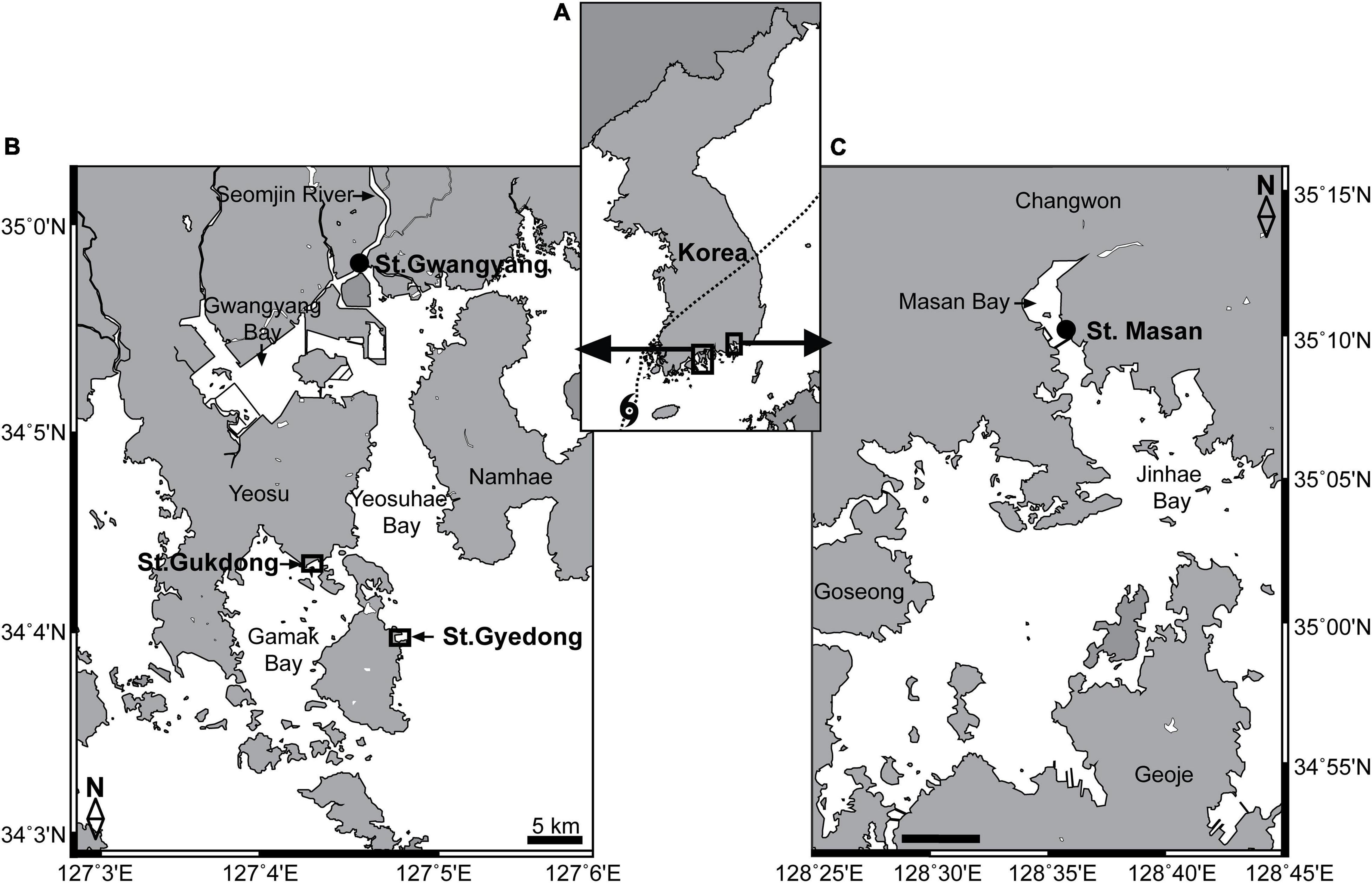
Figure 1. (A) Locations of the study areas in the South Sea of Korea. (B) Stations for seawater sample collection in Gamak Bay (St. Gukdong) and Yeosuhae Bay (St. Gyedong) and the station for automated seawater quality monitoring data acquisition in Gwangyang Bay (St. Gwangyang). (C) Station for the automated seawater quality monitoring data acquisition in Masan Bay (St. Masan). The dotted line in panel (A) indicates the path of the Danas typhoon on July 20, 2019.
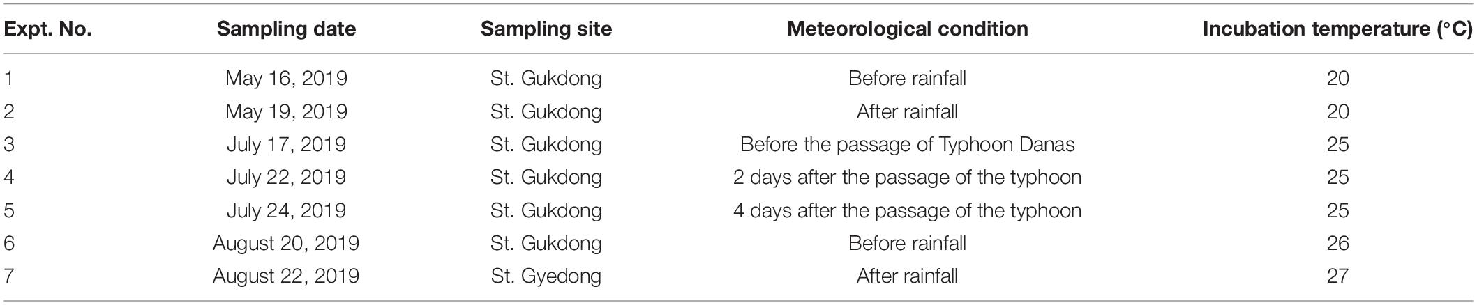
Table 1. Meteorological conditions when the seawater samples were collected from Station Gukdong and Station Gyedong in 2019 and their incubation conditions.
Experimental Procedures
Seawater collected on each sampling date was gently mixed and evenly distributed into 2 L polystyrene bottles (JetBiofiltration Co., Ltd, Guangzhou, China). All bottles incubated under each condition were set up in triplicates and placed in temperature-controlled chambers set to the ambient water temperature (±2°C; Table 1). These bottles were capped loosely and then incubated for 10 days at 100 μmol photons m–2 s–1 under a 14 h:10 h light:dark cycle using light-emitting diodes (LEDs; FS-075MU, 6500K; Suram Inc., Suwon, South Korea). Based on the light intensity at which the maximum growth rates of many phytoplankton occurred and the effects of photoinhibition on phytoplankton growth were minimized, a light intensity of 100 μmol photons m–2 s–1 was used. This ensured that light was not a limiting factor in this study. For example, the light intensities at which the maximum growth rates were observed were >10 μmol photons m–2 s–1 for the dinoflagellate Paragymnodinium shiwhaense (Jeong et al., 2018), >58 μmol photons m–2 s–1 for the dinoflagellate Alexandrium pohangense (Lim et al., 2019), >70 μmol photons m–2 s–1 for the diatom Leptocylindrus danicus (Verity, 1982), >80 μmol photons m–2 s–1 for the diatoms Skeletonema costatum, Thalassiosira minima, and Thalassiosira eccentrica, and the dinoflagellates Protodinium simplex, Scrippsiella sweeneyae, and Prorocentrum micans (Chan, 1978), and >90 μmol photons m–2 s–1 for the dinoflagellate Margalefidinium polykrikoides (Kim et al., 2004). Moreover, the light intensities at which the negative growth rates of phytoplankton due to photoinhibition occurred were >123 μmol photons m–2 s–1 for the dinoflagellate Karenia brevis (Magaña and Villareal, 2006), >135 μmol photons m–2 s–1 for the dinoflagellate Tripos furca (Nordli, 1957), >247 μmol photons m–2 s–1 for the dinoflagellate Takayama helix (Ok et al., 2019), and >317 μmol photons m–2 s–1 for the diatoms Ditylum brightwellii and Thalassiosira sp. (Brand and Guillard, 1981). Daylength in the study area from May to August is approximately 13–14.5 h (Sunrise-Sunset, 2021).4 Thus, this light condition can simulate the natural environment in the study area.
Subsampling and Component Analyses
Subsampling was conducted daily in all experimental seawaters except for the one collected on May 16, 2019 (every two days) to quantify the Chl-a and nutrient concentrations and the planktonic protist abundance.
For Chl-a analysis, a 20 mL aliquot taken from each bottle was filtered through a GF/F filter (Whatman Inc., Clifton, NJ, United States), and the filtered membrane was placed in a 15 mL conical tube and stored below −20°C. Then, 10 mL of 90% acetone was added to the conical tube containing the sample. The conical tubes were sonicated for 10 min, wrapped in aluminum foil to avoid light, stored in a 4°C chamber overnight, and centrifuged, and then 5 mL of the supernatant was taken from each tube and measured using a 10-AU Turner fluorometer (Turner Designs, Sunnyvale, CA, United States). For nutrient analysis, a 20 mL aliquot of the filtrate samples was stored in polyethylene vials below −20°C. The concentrations of nitrate plus nitrite (hereafter nitrate or NO3), ammonium (NH4), phosphate (PO4), and silicate (SiO2) in the seawater samples were measured using a 4-channel nutrient auto-analyzer (QuAAtro, SEAL Analytical GmbH, Norderstadt, Germany; Bran+Luebbe Analyzing Technologies, 2004a, b, 2005; SEAL Analytical GmbH, 2005).
To quantify the abundance of dominant planktonic protists, a 10 mL aliquot was taken from each bottle and fixed with 5% acidic Lugol’s solution (Sournia, 1978). Each dominant taxon was enumerated by counting >200 or all cells for each species in a Sedgewick-Rafter chamber using an inverted microscope (BX53, Olympus, Japan) at a magnification of ×100–200.
To convert the abundance (cells mL–1) of dominant planktonic protists to biomass (ng C mL–1), the cellular carbon content of each taxon was obtained from the literature or estimated from its biovolume according to Menden-Deuer and Lessard (2000). The biovolume of each taxon was calculated using Hillebrand et al. (1999) after measuring the cell length and width, or diameter and height of ≥5 cells of the taxon.
Data Analysis and Equation Development
The concentrations of NO3, NH4, PO4, SiO2, and Chl-a were measured every sampling day and dissolved inorganic nitrogen (NO3+NH4; DIN) was calculated from these data. When Chl-a increased, the magnitude of the Chl-a peak (i.e., the maximum Chl-a) and the time elapsed until the Chl-a peak occurred (Daypeak) were determined. When Chl-a decreased, the initial Chl-a was regarded as the Chl-a peak. Using the data, the ratio of the initial NO3 to Chl-a [μM (μg L–1)–1] was calculated by dividing the initial NO3 by the initial Chl-a for each incubated seawater sample. This value was also calculated as a unitless ratio, multiplied by the molecular weight of N (=14 g mol–1) to convert μmol L–1 (=μM) to μg L–1. The growth rate (μ, day–1) of the phytoplankton community was calculated as follows:
When the Chl-a decreased, the growth rate was allocated to zero.
To develop equations for the magnitude of the Chl-a peak of the phytoplankton community, four different simple linear regressions were analyzed: the Chl-a peak versus the initial NO3; the Chl-a peak versus the ratio of the initial NO3 to Chl-a; the ratio of the peak-to-initial Chl-a versus the initial NO3; and the ratio of the peak-to-initial Chl-a versus the ratio of the initial NO3 to Chl-a. Furthermore, to develop an equation for Daypeak, four different simple linear regressions were also analyzed: Daypeak versus the natural log of the initial NO3; Daypeak versus the natural log of the ratio of the initial NO3 to Chl-a; the growth rate versus the natural log of the initial NO3; and the growth rate versus the natural log of the ratio of the initial NO3 to Chl-a. The growth rate was used as a variable because the growth rate equation itself includes time. Similar analyses were conducted using NH4, DIN, PO4 and SiO2, as well as the ratio of the initial NO3 to PO4 and the ratio of the initial NO3 to SiO2. To apply this method at a species level, the peak abundance of Skeletonema costatum of each seawater sample during bottle incubation was determined. The goals were to develop equations for predicting bloom outbreaks of each species and to assess the contribution of each bloom species of interest to the phytoplankton community. The cellular chlorophyll-a content of S. costatum was obtained from Hitchcock (1980). The estimated Chl-a peak and Daypeak of S. costatum were determined using the analyses described above.
Linear regression equations were established by fitting the data using DeltaGraph (SPSS Inc., Chicago, IL, United States). These equations were solved to deduce the Chl-a peak and Daypeak.
Comparison of the Predicted and Field Data
To test whether the bloom prediction equations obtained from the present study (in sections “Correlations Between the Variables Related to the Chl-a Peak” and “Correlations Between Variables Related to the Timing of Chl-a Peaks”) can be used to predict bloom outbreaks in the field, in situ time-series data of the automated seawater quality monitoring system in the South Sea of Korea (St. Gwangyang and St. Masan; Figure 1) were obtained from the Marine Environment Information System (2021).5 Data from May to October in 2016–2019 were used because the water temperatures during this period were similar to those of our incubation experiments using the seawaters collected from St. Gukdong and St. Gyedong. The values of NO3, Chl-a, salinity, and water temperature measured at five-minute intervals in a day were each averaged to obtain the mean value of the day (Supplementary Table 1). Based on these monitored data, the following steps were conducted (Supplementary Figure 1). First, the Chl-a peak was found when the Chl-a exceeded 5 μg L–1 with an increasing trend, assuming the criterion of a phytoplankton bloom as 200 ng C mL–1 and a carbon to Chl-a ratio of 40 (Peterson and Festa, 1984; Jeong et al., 2013). Second, Chl-a and NO3 levels, prior to reaching the Chl-a peak, were selected. Third, the time elapsed until the Chl-a peak occurred (Daypeak) was counted. Fourth, using the selected NO3 and Chl-a data and the equations developed in this study (in Sections “Correlations Between the Variables Related to the Chl-a Peak” and “Correlations Between Variables Related to the Timing of Chl-a Peaks”), the predicted values were calculated for each date and then compared with the actual Chl-a peak or Daypeak using linear regression analyses. Data were not used when the daily average salinity changed by >2 because it indicated seawater with different nutrient conditions introduced from the river or large streams.
Statistical Analysis
Pearson’s correlation was used to examine the relationships between variables (Pearson, 1895). All statistical analyses were performed using SPSS (version 25.0; IBM Corp., Armonk, NY, United States). The significance criterion was set at 0.05.
Results
Physical and Chemical Properties of the Seawater Samples
During the study period in 2019, water temperature, precipitation, and salinity varied considerably whereas pH and dissolved oxygen (DO) did not (Figure 2): the water temperature ranged from 18.2°C on May 19 to 26.6°C on August 22 (Figure 2A); the precipitation summed for 7 days was 274.1 mm on July 22 and July 24 but <100 mm on the remaining dates (Figure 2B); the salinity was 24.36 and 29.10 on July 22 and July 24, respectively, but exceeded 29.9 on the remaining dates, with a maximum of 33.78 on May 16 (Figure 2C); the pH was 7.89 on July 22 but exceeded 7.90 on the remaining dates, with a maximum of 8.10 on August 22 (Figure 2D); and the DO was 5.01 mg L–1 on July 24 but exceeded 5.4 mg L–1 on the remaining dates with a maximum of 6.07 mg L–1 on May 16 (Figure 2E).
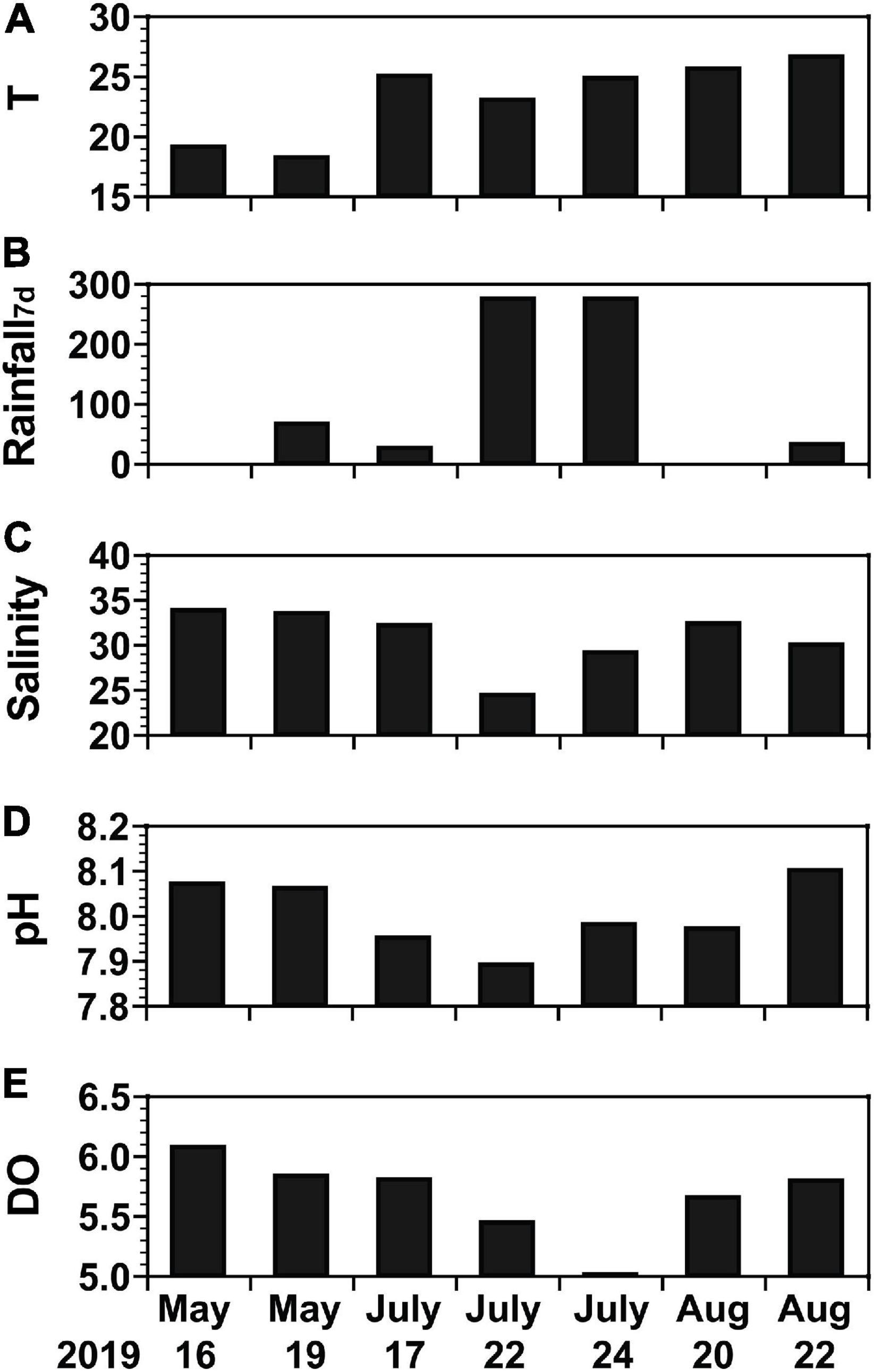
Figure 2. Background environmental conditions of water samples from May 16 to August 22, 2019. (A) Temperature (T, °C), (B) amount of rainfall for 7 days [Rainfall7d, mm (7 d)− 1], (C) salinity, (D) pH, and (E) dissolved oxygen (DO, mg L− 1).
There was 65.8 mm of rainfall between May 17 and May 18, 274.1 mm between July 17 and July 21, and 31.9 mm between August 21 and 22. Typhoon Danas passed through Korea and affected the study area on July 20 (Figure 1A). The maximum wind speed during the passage of the typhoon in the study area was 21.3 m s–1.
Dominant Protist Species at the Beginning of Incubation
At the beginning of each bottle incubation experiment, the most dominant planktonic protist species based on carbon biomass in chronological order was the diatom Cylindrotheca closterium on May 16, the photosynthetic dinoflagellate T. furca on May 19, the tintinnid ciliate Tintinnopsis sp. on July 17 and July 22, the diatoms Pseudo-nitzschia pungens on July 24 and Chaetoceros curvisetus on August 20, and the photosynthetic ciliate Mesodinium rubrum on August 22 (Figures 3A–G).
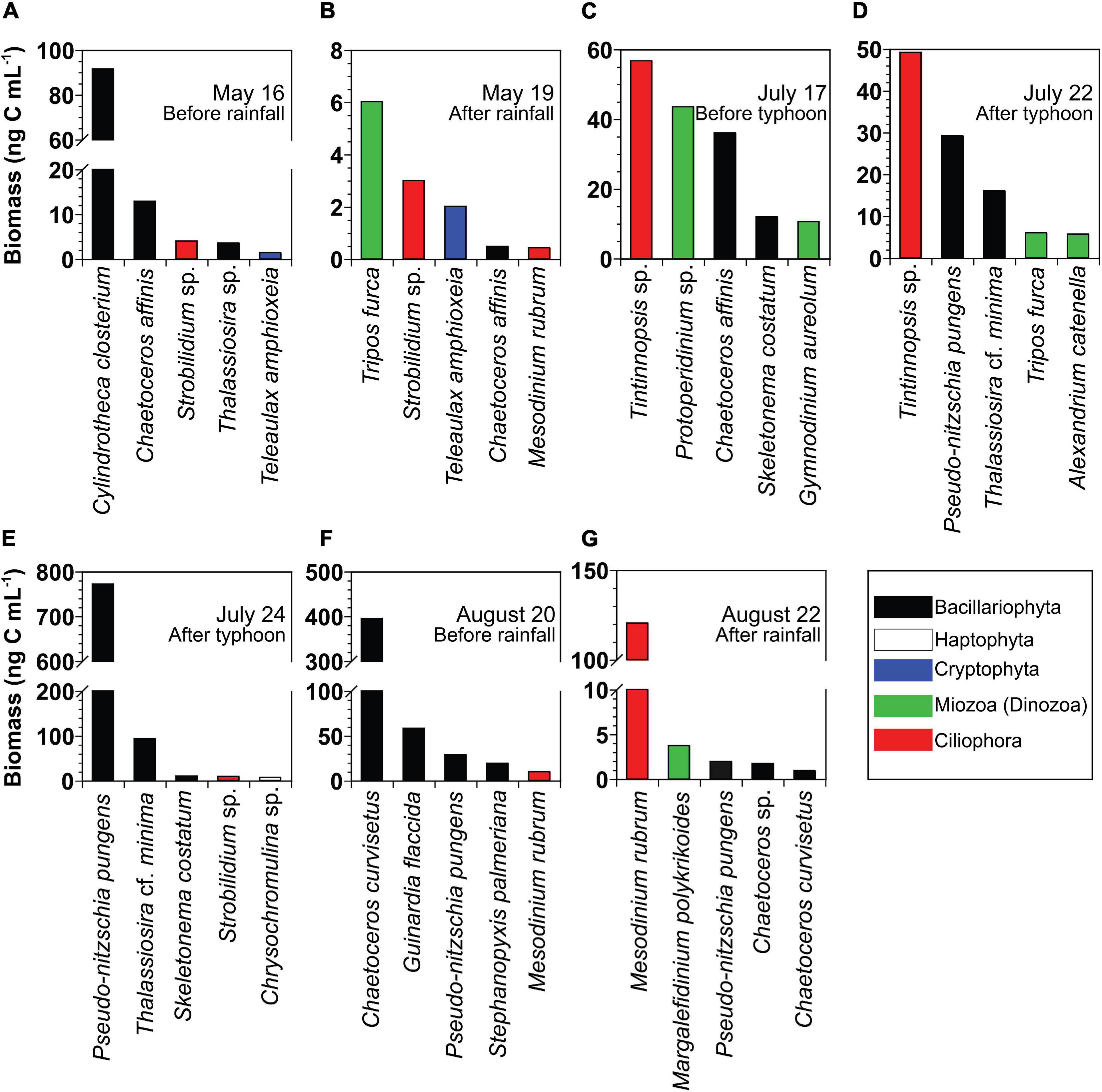
Figure 3. (A–G) Biomass of the five dominant planktonic protists at the beginning of the incubation of the seven different seawater samples collected from St. Gyedong (August 22) or St. Gukdong (the remaining dates) in 2019. To convert the unit from cell abundance to biomass, the cellular carbon content of each dominant species was obtained from Goldman (1993), Olenina et al. (2006), Yoo et al. (2010); Lee et al. (2014), Harrison et al. (2015), and Lim et al. (2019). The cellular carbon content of Alexandrium catenella was calculated from the equivalent spherical diameter in Kang et al. (2018). The cellular carbon contents of Chrysochromulina sp. (0.004 ng C cell− 1), Chaetoceros sp. (0.001 ng C cell− 1), Thalassiosira cf. minima (0.02 ng C cell− 1), Thalassiosira sp. (0.10 ng C cell− 1), Protoperidinium sp. (1.81 ng C cell− 1), Strobilidium sp. (1.00 ng C cell− 1), and Tintinnopsis sp. (3.78 ng C cell− 1) were calculated from the biovolume in this study.
Initial Nutrient and Chl-a Concentrations
The initial concentrations of NO3, NH4, and DIN of the experimental seawater ranged from 0.6 μM (August 20) to 39.7 μM (July 22), from 0.1 μM (July 17) to 10.2 μM (July 22), and from 1.5 μM (July 17) to 49.9 μM (July 22), respectively (Figures 4A–C). The initial PO4 concentrations ranged from 0.1 μM (July 24) to 1.1 μM (July 22; Figure 4D), while the initial SiO2 concentrations varied from 4.4 μM (August 20) to 93.4 μM (July 22; Figure 4E). The initial Chl-a concentrations ranged from 0.8 μg L–1 (May 19) to 24.5 μg L–1 (July 24; Figure 4F).
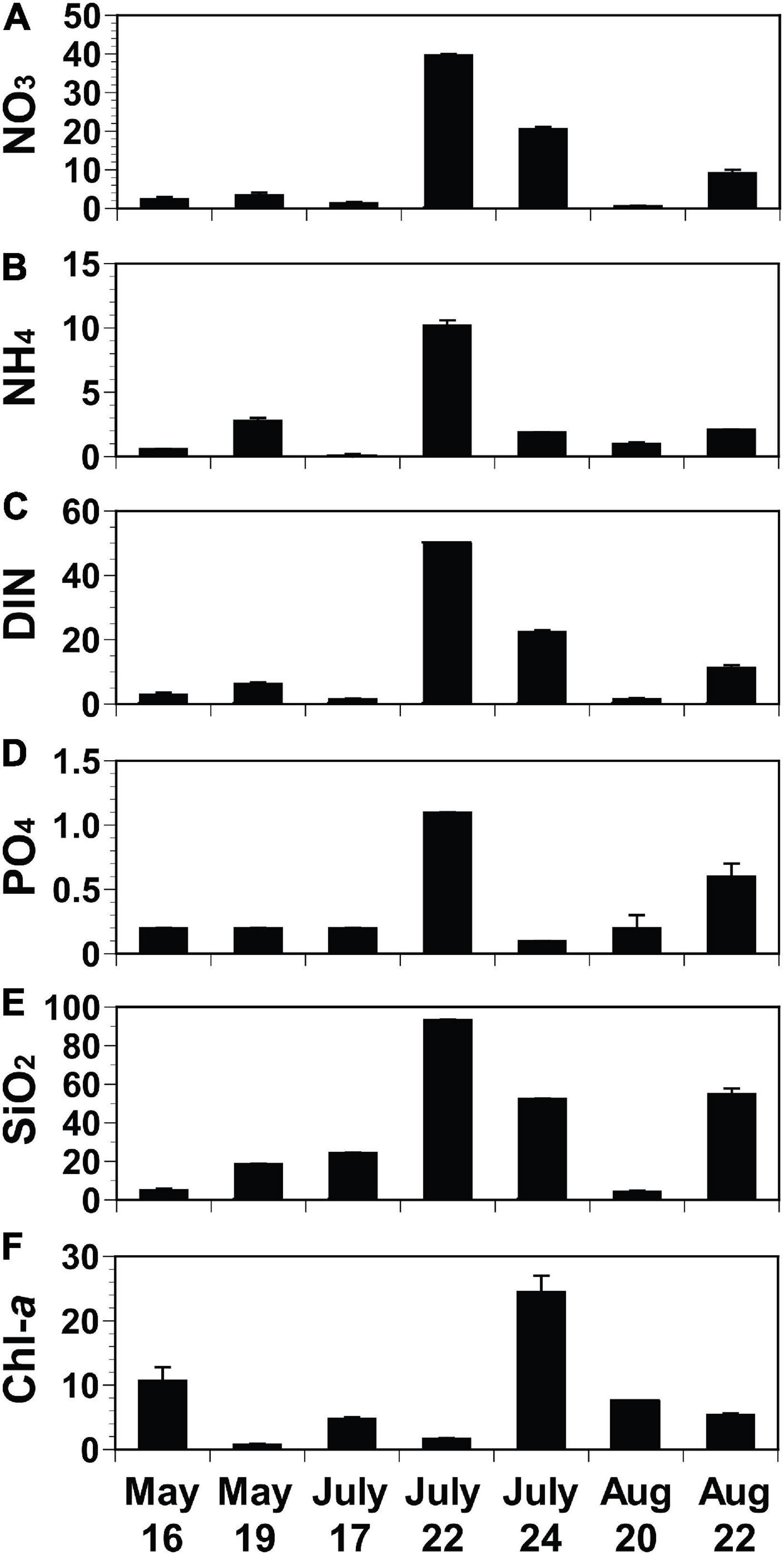
Figure 4. Initial concentrations of nutrients (A–E; NO3, NH4, DIN, PO4, and SiO2; μM) and chlorophyll-a (F; Chl-a; μg L− 1) of each seawater collected from St. Gyedong (August 22) or St. Gukdong (the rest dates) in 2019. Vertical symbols represent treatment means ± 1 SE.
Variations in Nutrient and Chl-a During Incubation
Chl-a showed two different patterns as incubation time progressed (Figures 5A–G); first, it decreased in the seawater samples from May 16, July 17, and August 20 (Figures 5A–C); second, it increased to a peak, but then decreased later in the rest of the samples as NO3, NH4, DIN, PO4, or SiO2 became depleted (Figures 5D–G).
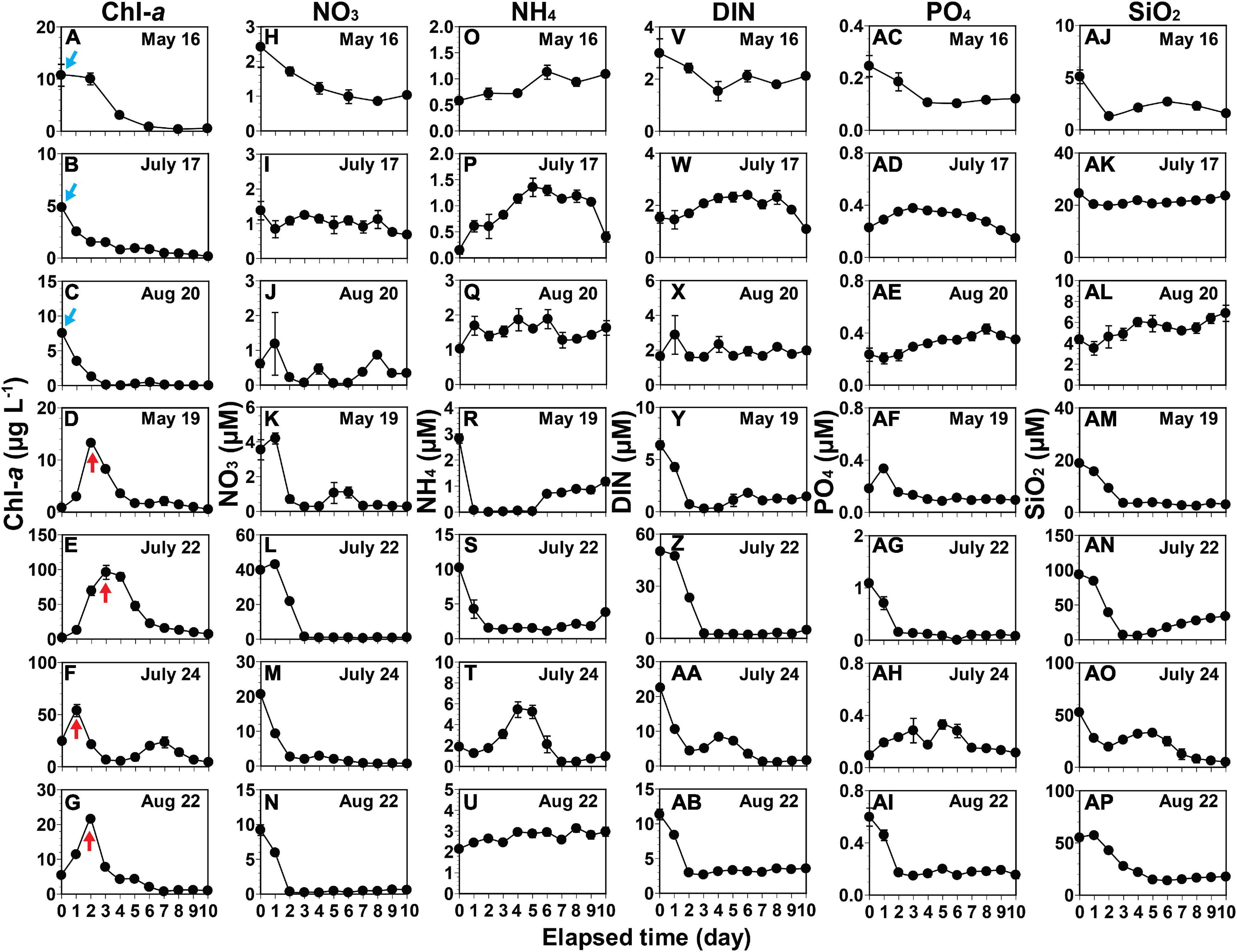
Figure 5. Variations in the concentrations of chlorophyll-a (Chl-a) and nutrients. Chl-a (A–G), nitrate (NO3) (H–N), ammonium (NH4) (O–U), dissolved inorganic nitrogen (DIN) (V–AB), phosphate (PO4) (AC–AI), and silicate (SiO2) (AJ–AP) during incubation of seawaters. A blue arrow indicates the highest Chl-a in the seawater where any increase in Chl-a did not occur during incubation. A red arrow indicates the Chl-a peak in the seawater where increases in Chl-a occurred during incubation. The date in each box indicates the sampling date of the seawater collected from St. Gyedong (August 22) or St. Gukdong (the remaining dates) in 2019. Vertical symbols represent treatment means ± 1 SE.
Chlorophyll-a decreased during incubation when the initial NO3 concentrations were ≤2.4 μM (Figures 5A–C,H–J and Supplementary Figure 2A). In contrast, Chl-a increased when the initial NO3 concentrations were ≥3.5 μM (Figures 5D–G,K–N and Supplementary Figure 2B). Chl-a decreased when the initial NH4 concentrations were ≤1.0 μM, while Chl-a increased when the concentrations were ≥2.1 μM (Figures 5O–Q,R–U). Furthermore, Chl-a decreased when the initial DIN concentrations were ≤3 μM but increased when the concentrations were ≥6.4 μM (Figure 5V–X,Y–AB). Chl-a decreased during incubation when the initial PO4 concentrations were ≤0.3 μM (Figures 5A–C,AC–AE) with one exception: Chl-a increased when the initial PO4 concentration was 0.1 μM in the seawater on July 24 (Figures 5F,AH). Chl-a also decreased when the initial SiO2 concentrations were ≤24.5 μM (Figures 5A–C,AJ–AL) with one exception: Chl-a increased when the initial SiO2 concentration was 18.7 μM in the seawater of May 19 (Figures 5D,AM).
Correlations Between the Variables Related to the Chl-a Peak
The Chl-a peak of the phytoplankton community was in between 4.6 and 114 μg L–1 (Figures 6A,B). The ratio of the peak-to-initial Chl-a of the phytoplankton community varied from 1.0 to 61.4 (Figures 6C,D). The ratio of the initial NO3 to Chl-a of the phytoplankton community ranged from 0.1 to 24.2 μM (μg L–1)–1 (equivalent to 0.8–339 in a unitless ratio, respectively; Figures 6B,D).
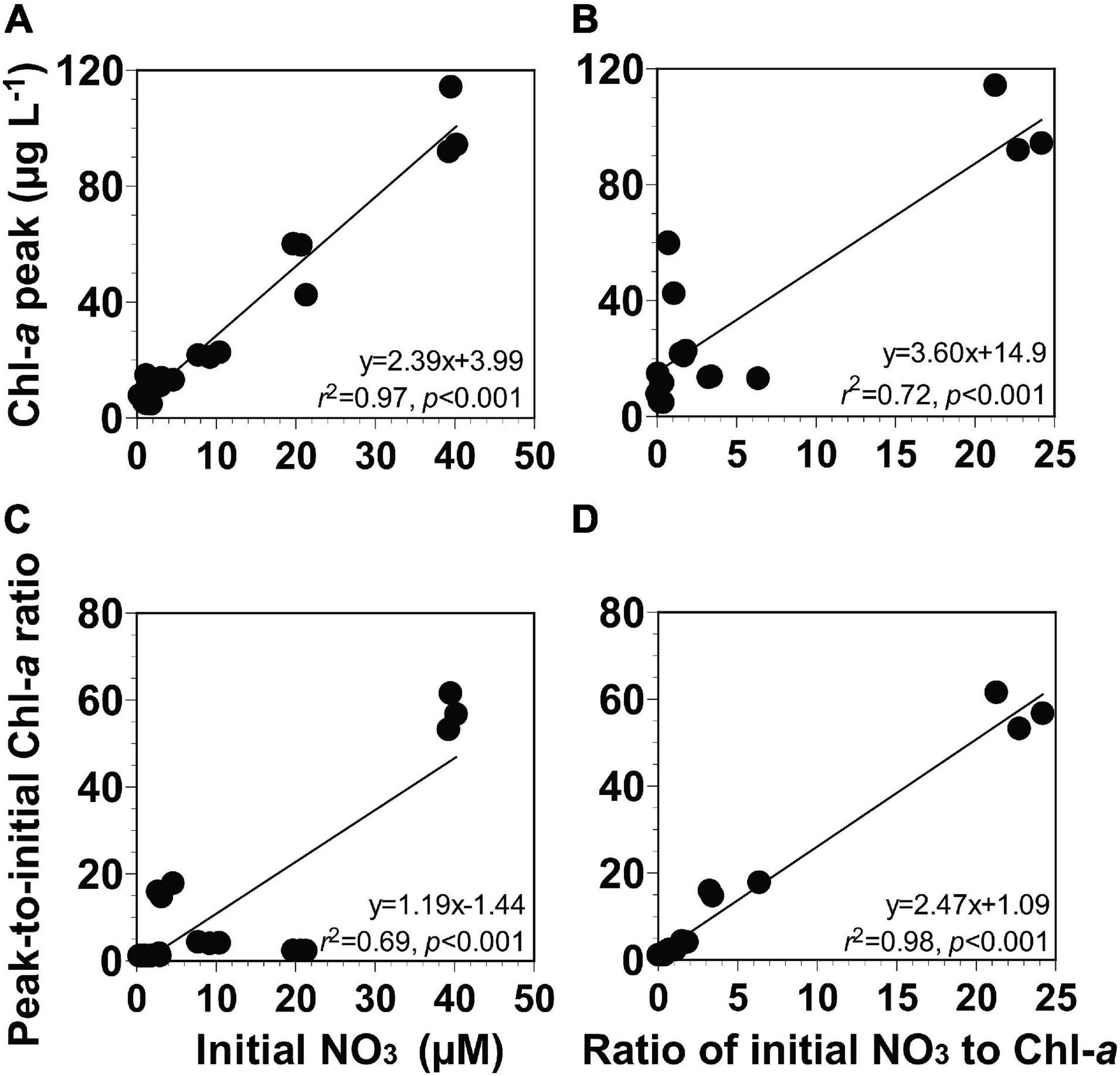
Figure 6. (A,B) Chl-a peak (μg L− 1) or (C,D) peak-to-initial Chl-a ratio of the phytoplankton community as a function of the initial NO3 (μM) or the ratio of initial NO3 to Chl-a [μM (μg L− 1)− 1]. The ratio of initial NO3 to Chl-a [μM (μg L− 1)− 1] in panels (B,D) can be described as a unitless ratio by multiplying it with 14. Data were obtained from the seven experiments incubating seawater samples collected from St. Gukdong and St. Gyedong in 2019.
To develop equations for the magnitude of the Chl-a peak using the initial NO3 or the ratio of the initial NO3 to Chl-a, four different linear regressions between two variables were analyzed (see section “Data Analysis and Equation Development”). The Chl-a peak of the phytoplankton community was significantly correlated with the initial NO3 concentration and the ratio of the initial NO3 to Chl-a (Figures 6A,B). The ratio of peak-to-initial Chl-a of the phytoplankton community was also significantly correlated with the initial NO3 and with the ratio of initial NO3 to Chl-a (Figures 6C,D). Equations (Eqs 1–4 in Table 2) for calculating the Chl-a peak of the phytoplankton community were obtained from linear regressions in Figure 6.
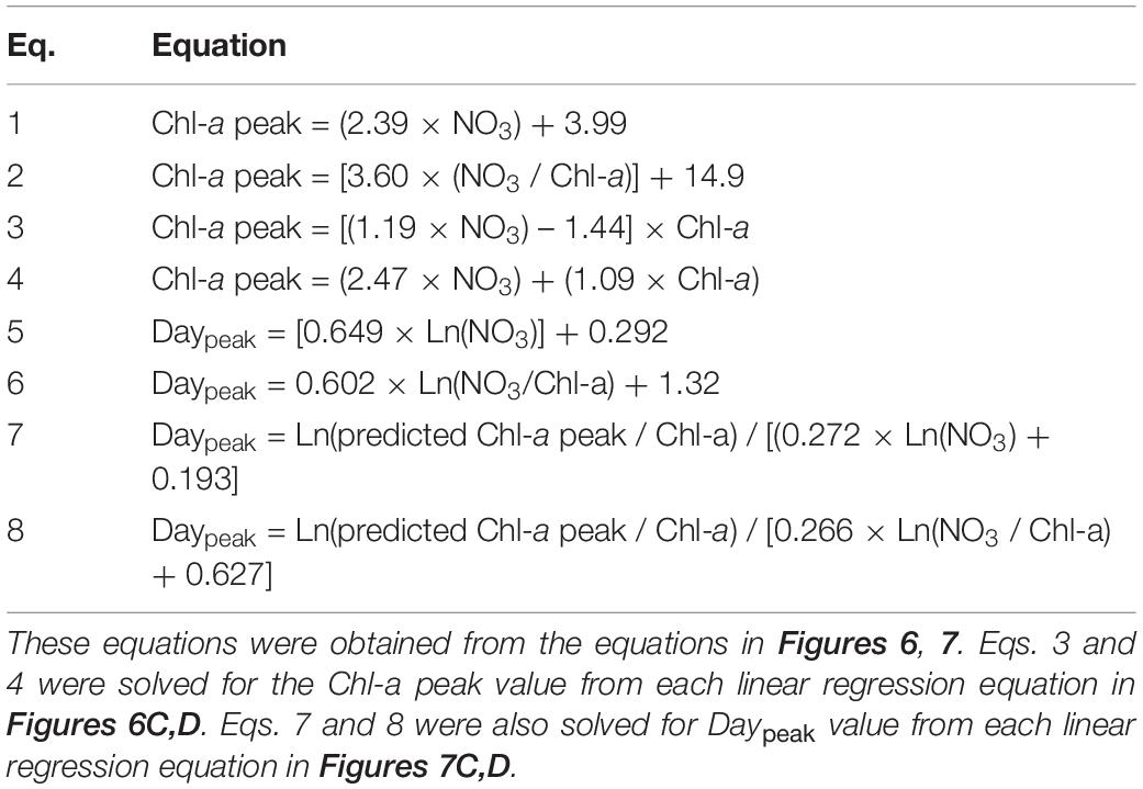
Table 2. Equations for calculating the peak chlorophyll-a concentration (Chl-a peak, μg L–1) of the phytoplankton community and the day elapsed until the Chl-a peak occurred (Daypeak; day).
These types of correlations were significant when NH4, DIN, PO4, and SiO2 were used (Supplementary Figures 3, 4). However, the Chl-a peak or the ratio of the peak-to-initial Chl-a of the phytoplankton community was not significantly correlated with the ratio of the initial NO3 to PO4 and the ratio of the initial NO3 to SiO2 (Supplementary Figure 5).
Correlations Between Variables Related to the Timing of Chl-a Peaks
In these incubation experiments, the elapsed day until the Chl-a peak of the phytoplankton community occurred (Daypeak) ranged from days 0 to 4, (Figures 7A,B). Furthermore, the growth rates of the phytoplankton community ranged from 0.0 to 1.4 day–1 (Figures 7C,D).
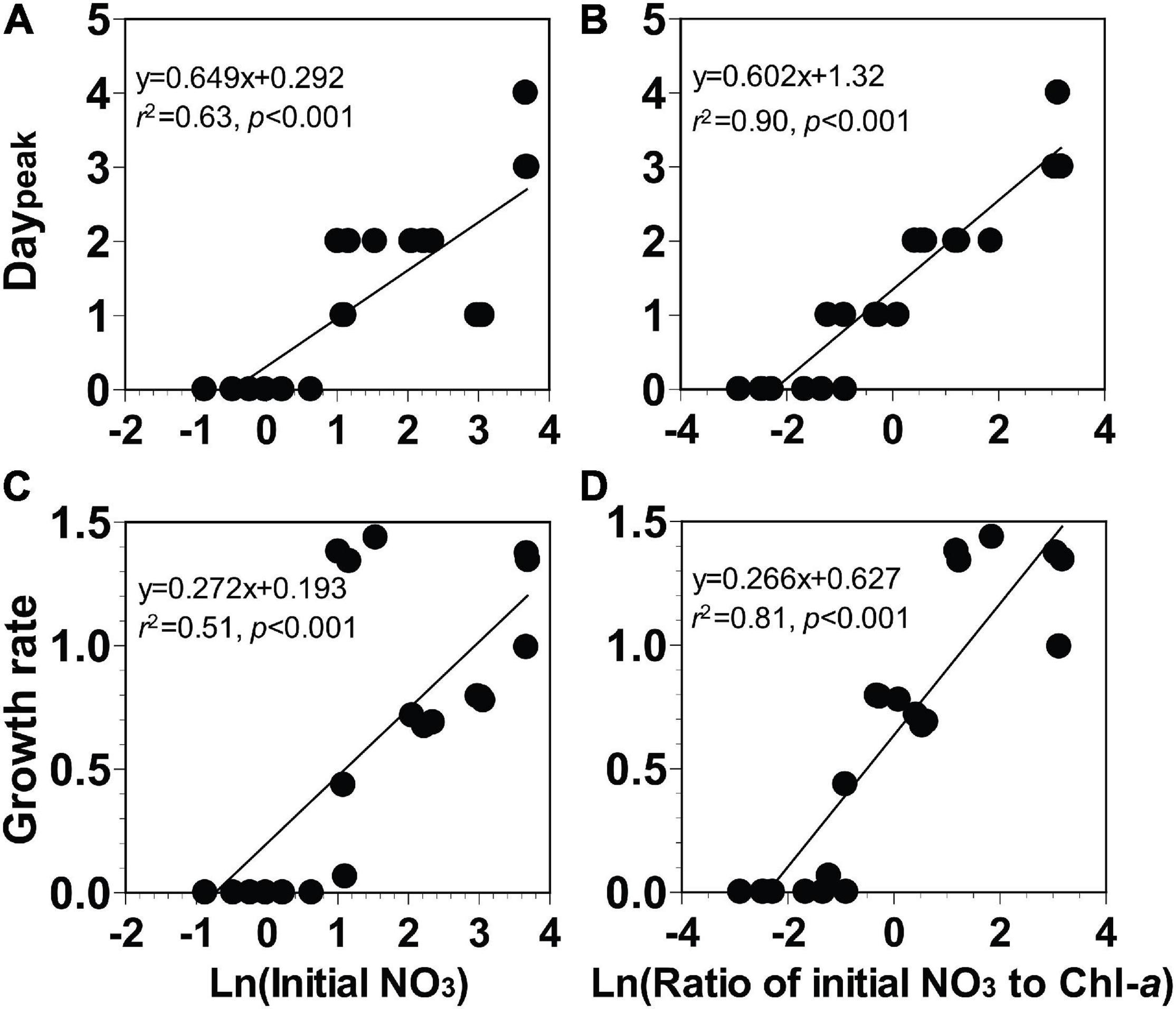
Figure 7. (A,B) The elapsed day until peak chlorophyll-a occurred (Daypeak, day) or (C,D) growth rate of the phytoplankton community (day− 1) as a function of the natural log of the initial NO3 (Ln μM) or the natural log of the ratio of the initial NO3 to Chl-a [Ln μM (μg L− 1)− 1]. Data were obtained from the seven experiments incubating seawater collected from St. Gukdong and St. Gyedong in 2019.
To develop equations for determining Daypeak using the natural log of the initial NO3 or the natural log of the ratio of initial NO3 to Chl-a, four different linear regressions between two variables were analyzed (see section “Data Analysis and Equation Development”). Daypeak of the phytoplankton community was significantly correlated with the natural log of the initial NO3 and with the natural log of the ratio of the initial NO3 to Chl-a (Figures 7A,B). The growth rate of the phytoplankton community was also significantly correlated with the natural log of the initial NO3 and with the natural log of the ratio of the initial NO3 to Chl-a (Figures 7C,D). Equations (Eqs 5–8 in Table 2) for calculating Daypeak were obtained from the equations of linear regressions in Figure 7.
These types of correlations were significant when NH4, DIN, and SiO2 were used, however, this was not always the case when PO4 was used (Supplementary Figures 6, 7). Moreover, Daypeak or growth rate of the phytoplankton community was significantly correlated with the natural log of the ratio of initial NO3 to PO4 but not with the ratio of the initial NO3 to SiO2 (Supplementary Figure 8).
Comparison of the Predicted and Field Values of Chl-a Peak and Daypeak
The ranges of the daily average values of the water temperature, salinity, NO3, and Chl-a in St. Gwangyang and St. Masan at the selected dates in 2016–2019 were different from those of St. Gukdong and St. Gyedong (Table 3 and Supplementary Table 1). The daily average water temperature ranges at St. Gwangyang (17.9–31.2°C) and St. Masan (16.5–30.6°C) were greater than those at St. Gukdong and St. Gyedong (18.2–26.6°C). The maximum values of the daily average salinity at each station were slightly different, but the minimum values at St. Gwangyang (5.1) and St. Masan (19.1) were much lower than those at St. Gukdong and St. Gyedong (24.4). The ranges of the daily average NO3 concentration at St. Gukdong and St. Gyedong (0.6–39.7 μM) were much greater than those at St. Gwangyang (0.6–16.1 μM) and St. Masan (0.1–7.7 μM). However, the ranges of the daily average Chl-a concentration at St. Gwangyang (1.1–49.5 μg L–1) and St. Masan (0.3–36.8 μg L–1) were much wider than those at St. Gukdong and St. Gyedong (0.8–24.5 μg L–1).
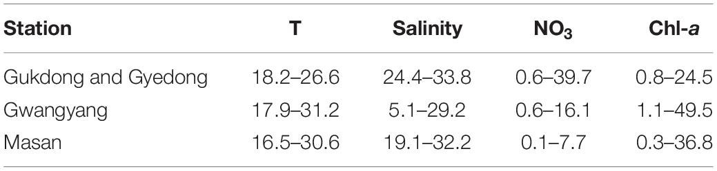
Table 3. Comparisons of water temperature (T, °C), salinity, NO3 (μM), and initial chlorophyll-a (Chl-a, μg L–1) in the seawater samples used for the incubation experiments (St. Gukdong and St. Gyedong) and the data obtained from the monitoring sites (St. Gwangyang and St. Masan) in the selected periods between 2016 and 2019 in the South Sea of Korea.
Applying Eqs 1–3 from Table 2, the actual peak Chl-a value measured at St. Gwangyang or St. Masan and the combined actual Chl-a peak values from both stations were not always significantly correlated with the predicted peak Chl-a value (Figures 8A–I). By contrast, using Eq. 4, the predicted values of Chl-a peak showed significant correlations with the actual Chl-a peak (Figures 8J–L). The root mean square errors (RMSE) were 10.6, 9.2, and 11.6 μg L–1 for St. Gwangyang, St. Masan, and the combined data of the two stations, respectively. Thus, Eq. 4 was chosen as a best-fit equation to predict the Chl-a peak in the field.
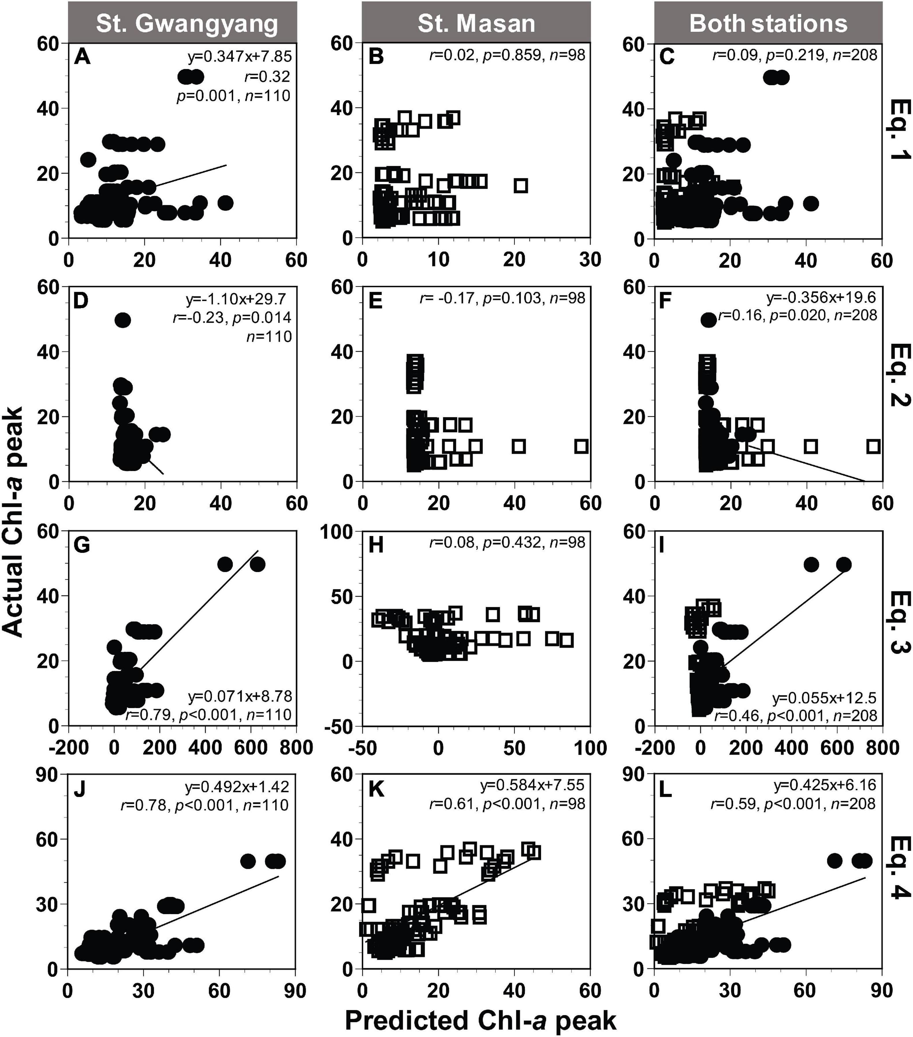
Figure 8. Comparison between the actual and predicted values of the Chl-a peak (μg L− 1) at St. Gwangyang (closed circle), St. Masan (open square), and both stations. The predicted Chl-a peak values calculated using concentrations of NO3 and Chl-a at each station and Eq. 1 (A–C), Eq. 2 (D–F), Eq. 3 (G–I), and Eq. 4 (J–L) in Table 2.
Based on Eqs 5, 7, and 8 from Table 2, the actual Daypeak data obtained from St. Gwangyang or St. Masan and the combined data of the two stations were not always significantly correlated with the predicted Daypeak (Figures 9A–C,G–L). On the other hand, with Eq. 6, the actual Daypeak data were significantly correlated with the predicted Daypeak (Figures 9D–F). The RMSE was all 1 day for St. Gwangyang, St. Masan, and the combined data of the two stations. Thus, Eq. 6 was selected as a best-fit equation to predict Daypeak in the field.
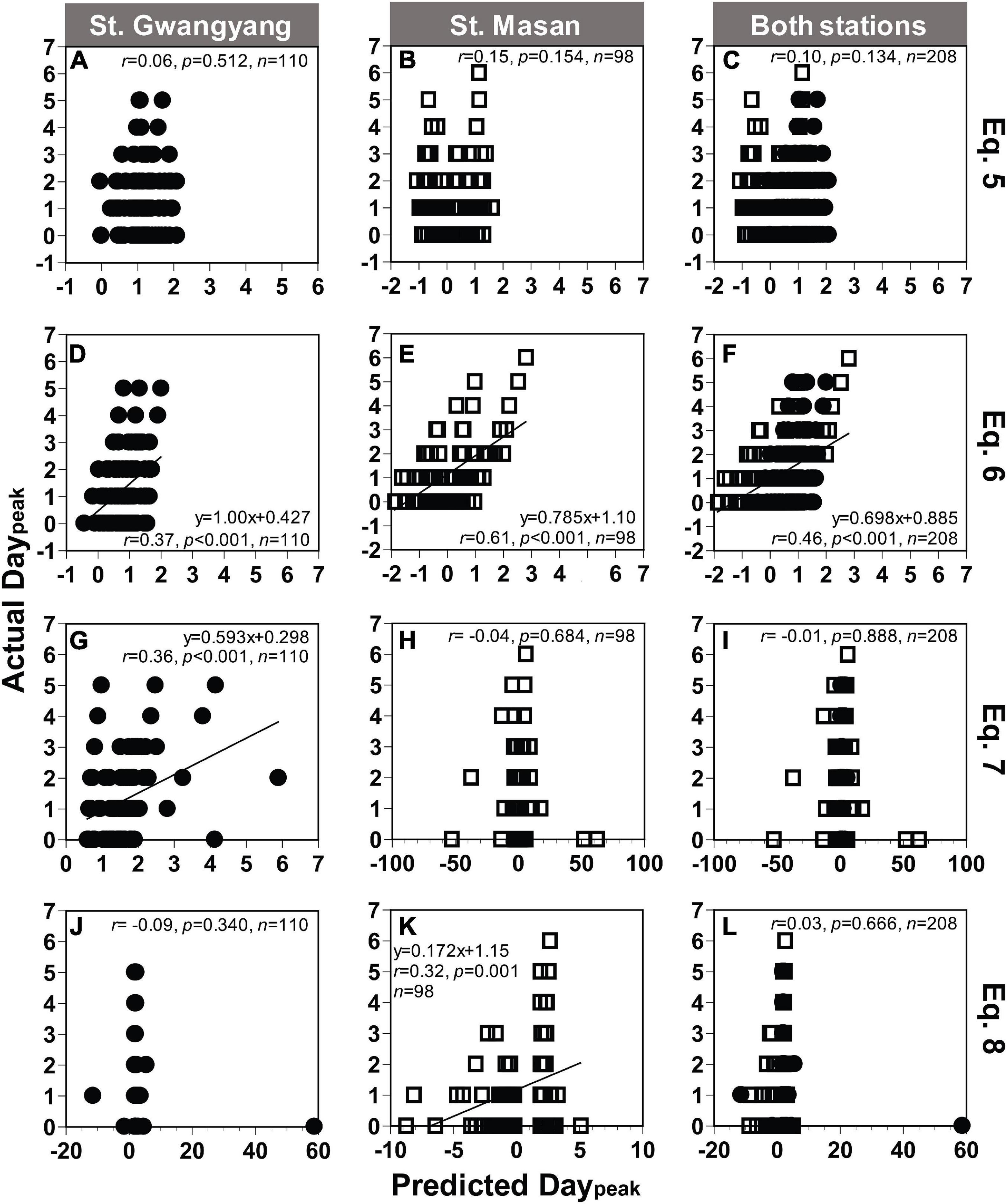
Figure 9. Comparison between the actual and predicted values of the day elapsed until the Chl-a peak occurred (Daypeak) at St. Gwangyang (closed circle), St. Masan (open square), and both stations. The predicted Daypeak values calculated using concentrations of NO3 and Chl-a at each station and Eq. 5 (A–C), Eq. 6 (D–F), Eq. 7 (G–I), and Eq. 8 (J–L) in Table 2. Predicted Daypeak in panels (G–L) were calculated using the predicted Chl-a peak from Eq. 4.
These comparisons were also made on Eqs 9–16 for in situ NH4 data and Eqs 17–24 for in situ DIN data (Supplementary Tables 1–3). The actual peak Chl-a values measured at St. Gwangyang or St. Masan and the combined actual peak Chl-a values from both stations were significantly correlated with the predicted values calculated using Eq. 11, 19, and 20 (Supplementary Figures 9, 10). The predicted Daypeak values were significantly correlated with the actual values when Eqs. 13 or 14 and Eqs. 21 or 22 were used (Supplementary Figures 11, 12). Therefore, any type of nitrogen data (NO3, NH4, or DIN concentrations) can be implemented to predict Daypeak values at St. Gwangyang or St. Masan.
Correlations Between Variables Related to the Magnitude and Timing of Skeletonema costatum
The Chl-a peak estimated for Skeletonema costatum ranged from 0.02 to 12.2 μg L–1 (Supplementary Figure 13A,B). The ratio of the peak-to-initial Chl-a estimated for S. costatum showed a spectrum of 1.0–90.4 (Supplementary Figures 13C,D). The ratio of the initial NO3 to Chl-a estimated for S. costatum had values in the range 2.7–1225.6 μM (μg L–1)–1 (equivalent to 38 and 17,158, in a unitless ratio, respectively; Supplementary Figures 13B,D).
Among the four types of linear regression (see section “Data Analysis and Equation Development”), there were significant correlations between the Chl-a peak estimated for S. costatum against the initial NO3 concentration and the ratio of the latter to the Chl-a concentration estimated for S. costatum against the ratio of the peak-to-initial Chl-a concentration estimated for S. costatum (Supplementary Figures 13A–D). These two correlations were always significant when NH4, DIN, PO4, or SiO2 were used (Supplementary Table 4). However, the Chl-a peak or the ratio of the peak-to-initial Chl-a concentration estimated for S. costatum was not significantly correlated with the ratio of initial NO3 to PO4 concentrations nor the ratio of initial NO3 to SiO2 concentrations (Supplementary Table 4).
In these incubation experiments, it took 0–4 days to reach the Chl-a peak (Supplementary Figures 13E,F). The growth rates of S. costatum ranged from 0.0 to 2.3 day–1 (Supplementary Figures 13G,H). Four different linear regressions between two variables were all significant when NO3, NH4, and DIN were applied (Supplementary Table 5 and Figures 13E–H). However, when PO4 was used, there were no significant correlations (Supplementary Table 5). Moreover, Daypeak or the growth rate of S. costatum was not always significantly correlated with the natural log of the ratio of initial NO3 to PO4 or initial NO3 to SiO2 (Supplementary Table 5).
Discussion
In this study, we successfully obtained equations to predict the magnitude and timing of peak phytoplankton blooms by following several critical steps: measuring daily fluctuations in the concentrations of nutrients and Chl-a in seawater enclosures; performing linear regression analyses between pairs of diverse variables described in section “Data Analysis and Equation Development.” The regression analyses led to the development of the eight equations for predicting the magnitude and timing of bloom peaks that are presented in this paper. Among these, Eq. 4 for magnitude and Eq. 6 for timing were significantly correlated with the observed actual data from St. Gwangyang and St. Masan. Thus, the magnitude and timing of bloom peaks can be easily identified a few days in advance. One week may be a critical time for aquafarmers to reduce economic losses due to red tides or harmful algal blooms. Moreover, NO3 and Chl-a in natural seawater samples can be evaluated in a few hours using a nutrient measuring instrument and a Chl-a sensor. Therefore, the method developed in this study is a quick way to predict the outbreaks of phytoplankton blooms.
The results of the present study showed that Chl-a decreased when the initial NO3 and NH4 concentrations were ≤2.4 and 1 μM (on May 16, July 17, and August 20), while it increased when the initial NO3 and NH4 concentrations were ≥3.5 and 2.1 μM (on the other dates), respectively. When NO3 concentration was ≤2.4 μM, the diatoms C. closterium (May 16) and C. curvisetus (August 20) most dominated the phytoplankton assemblages. The half-saturation constants of C. closterium and C. curvisetus for NO3 uptake are 0.4 and 0.6 μM, respectively (Anderson and Roels, 1981; Li et al., 2020). The half-saturation constant of C. closterium for NH4 uptake ranged from 0.1 to 0.3 μM, which was lower than the ambient NH4 concentration of 0.6 μM in the seawater where this diatom was dominant (May 16; Williams, 1964; Sunlu et al., 2006; Kingston, 2009). C. closterium and C. curvisetus were able to grow under these circumstances; however, the SiO2 concentrations on May 16 (5.1 μM) and August 22 (4.4 μM) were the lowest among the seawater samples collected during the study period. This meant that deficiencies in SiO2 concentration might be one of the reasons why these diatoms did not grow during incubation on those dates.
The dominant phototrophic protists in the seawaters used in this study, S. costatum, C. curvisetus, C. closterium, P. pungens, and T. furca, and the photosynthetic ciliate, M. rubrum, are commonly found in the seawater of many other regions (e.g., Tilstone et al., 1994; Marshall and Nesius, 1996; Zhang et al., 2015). Furthermore, they are known to often cause blooms in the study region and many other regions (e.g., Lips and Lips, 2017; Eom et al., 2021; Jeong et al., 2021). The naked ciliate Strobilidium spp. and the tintinnid ciliate Tintinnopsis spp. have also been reported to be common in the seawaters of many other regions (e.g., Dolan, 1991; Mironova et al., 2009). Thus, the results of the present study can be applied to other regions in which the dominant phototrophic and heterotrophic protists are similar to those of this study area. The method using the concentrations of nutrients and Chl-a, developed in this study, was able to predict the potential phytoplankton blooms even when microzooplankton such as Protoperidinium sp. and Tintinnopsis sp. were present in experimental seawaters. Moreover, although mesozooplankton might be removed through filtration of experimental seawaters, their grazing pressure on phytoplankton blooms has been reported to be low (Fiedler, 1982; Huntley, 1982; Stoecker and Sanders, 1985; Kim et al., 2013; Lee et al., 2017). Thus, grazing by mesozooplankton was not considered in this study.
The present study used a conversion factor of 14 to convert the unit from moles of nitrogen to gram because this factor has been most commonly used in previous studies (e.g., Baldock et al., 2004; Cosme et al., 2015). Some studies have empirically proved that 1 μM of nitrogen is equal to 1–2 μg L–1 of chlorophyll in Scottish coastal waters and San Francisco Bay Delta (Gowen et al., 1992; Glibert et al., 2014). Thus, 0.5–1 can also be used as a conversion factor to convert the unit depending on the region or the dominant phytoplankton species.
The reported growth rates of phytoplankton assemblages in temperate coastal waters showed a spectrum of 0.0–3.4 day–1 (Furnas, 1990 and references therein); the phytoplankton community growth rate in Loch Creran in Scotland (0.2–0.5 day–1), Celtic Sea (0.3–1.2 day–1), Southern California in US (0.3–1.3 day–1), Dabob Bay in US (0.0–0.9 day–1), and the east coast of the Izu Peninsula in Japan (0.9 day–1) were within the range of that of the present study (0.0–1.4 day–1). Moreover, the in situ growth rate of S. costatum in many other regions has been reported to have values between 1 and 4.1 day–1 (Furnas, 1990 and references therein); the in situ growth rates of this species in the Great Barrier Reef in Australia (2.2 day–1), Tampa Bay in US (1.0 day–1), and Trondhiem Fjord in Norway (1.0 day–1) were within the range of that in the present study (0.0–2.3 day–1). Thus, the method for predicting the timing of a bloom peak based on the growth rate can be used in regions where the growth rate of the phytoplankton community or S. costatum are similar.
In the present study, S. costatum was chosen as a representative species to determine Chl-a peaks and Daypeak at a species level. This species was present in all seawater samples collected during the study period. Furthermore, S. costatum is the most common red-tide diatom in the coastal waters of the countries that experience red tides (Jeong et al., 2021). Finally, S. costatum can inhibit the growth of the harmful dinoflagellate Margalefidinium polykrikoides, which has caused an annual economic loss of up to USD 60 million in Korea (Lim et al., 2014, 2015). Thus, if S. costatum blooms can be predicted accurately, the population dynamics of M. polykrikoides can also be determined. Taking this point into consideration, the initial nutrient-to-Chl-a ratio and the peak-to-initial Chl-a ratio of each species should be determined at the species level to develop methods for predicting blooms for each species. The range of the ratio of the initial NO3 to Chl-a estimated for S. costatum [2.7–1,226 μM (μg L–1)–1] was much wider than that of the total phytoplankton community [0.1–24.2 μM (μg L–1)–1]. This is because S. costatum was part of the phytoplankton community and diatoms such as S. costatum had lower concentrations of Chl-a than other types of phytoplankton (Hitchcock, 1982; Moal et al., 1987). Moreover, the range of peak-to-initial Chl-a ratio of S. costatum (1.0–90.4) was much wider than that of the phytoplankton community (1.0–61.4). This species grows faster than the other phytoplankton species that make up the phytoplankton community (Finenko and Krupatkina-Akinina, 1974).
The seawater samples for experiments collected from St. Gukdong and St. Gyedong had slightly different water temperature ranges than those at the validation sites (St. Gwangyang and St. Masan). However, the ranges of other environmental factors—such as salinity and Chl-a—were largely different between the sites for the experiments (St. Gukdong or St. Gyedong) and validation (St. Gwangyang or St. Masan). Moreover, interannual variations in diverse factors (e.g., salinity, temperature, mixing, or turbidity) were not considered in this study. Nevertheless, predictions of the magnitude and timing of the peaks of the blooms at the validation sites corresponded well with the actual measurements from May to October, for each year from 2016 to 2019. Thus, the method developed in this study can be used in other regions and periods having different ranges of environmental factors from those of the study sites.
Other types of nutrients (e.g., NH4, DIN, PO4, or SiO2) can also be used to predict peak bloom periods using the method described in this study, depending on the characteristics of the site of interest and the dominant bloom taxa. Some urbanized coastal and estuarine regions (e.g., Delaware Estuary, Neuse Estuary, San Fransico Estuary, Manila Bay, Scheldt Bay, Rhine Bay) or periods in a region, in particular, show high NH4 concentrations (Middelburg and Nieuwenhuize, 2000; Burkholder et al., 2006; Yoshiyama and Sharp, 2006; Chang et al., 2009; Parker et al., 2012a; Seeyave et al., 2013; Glibert et al., 2016). NH4 also contributes more to the growth of phytoplankton communities than NO3 in some regions (e.g., Dokai Bay, Santa Monica Bay, and Kaneohe Bay; Harvey and Caperon, 1976; Eppley et al., 1979; Tada et al., 2009), and many phytoplankton taxa that cause noxious blooms are associated with the reduced forms of nitrogen, including NH4 (Bates et al., 1993; Leong et al., 2004; Trainer et al., 2007; Seeyave et al., 2009; Killberg-Thoreson et al., 2014). In these cases, NH4 should be used as the main nutrient component to predict bloom peaks. The present study mainly used equations that were based on NO3 because DIN in seawater samples from the study area was dominated by NO3. Moreover, NO3 is a good indicator for predicting the magnitude and timing of algal bloom peaks for regions where diatoms are one of the most common species in regions like the sampling sites of this study because these species are preferentially NO3-users (Lomas and Glibert, 1999a, b, 2000; Kudela and Dugdale, 2000; Glibert et al., 2014, 2016).
Enclosure experiments have enabled the investigation of phytoplankton responses to environmental factors and the calculation of growth or nutrient uptake rates of phytoplankton, preventing physical mixing with surrounding waters (Pitcher et al., 1993; Kudela and Dugdale, 2000; Parker et al., 2012b; Lee et al., 2019b; Ferreira et al., 2020). However, results from the enclosure experiments are limited by differences in chemical (e.g., nutrients, dissolved gases), physical (e.g., wind-induced turbulence, light intensity), and biological variables (e.g., predators and prey) from nature, the so-called “bottle effects” (Veldhuis and Timmermans, 2007; Nogueira et al., 2014). The predicted Daypeak value may be lower than the actual Daypeak value because equations developed in this study may be affected by the absence of mixture or dilution in nature. Comparisons between the predicted and actual Daypeak values showed one-day differences at St. Gwangyang and St. Masan. Thus, a one-day time lag should be considered when using this equation (Eq. 6). Residence time is another important parameter for determining the timing of bloom outbreaks in nature, and it varies among regions (Delesalle and Sournia, 1992; De Sève, 1993; Phlips et al., 2012; Chen et al., 2013; Wan et al., 2013; Ralston et al., 2015; Glibert et al., 2018a). The residence time in Gamak Bay is approximately 11 days (Kim et al., 2016); this is greater than the highest Daypeak of 4 days obtained in the present study. Thus, residence time might not largely affect the equations derived from the results of the enclosure experiments in this study.
Models for predicting phytoplankton blooms have been developed using technological advances and knowledge accumulated over decades (McGillicuddy, 2010; Anderson et al., 2015; Franks, 2018; Zohdi and Abbaspour, 2019). However, there are still many challenges with this due to the complexity of the models involved and the difficulty of validating them; therefore, works combining laboratory and field studies are needed (Flynn and McGillicuddy, 2018). The present study combined laboratory and field work to improve the prediction of the magnitude and timing of phytoplankton blooms. Moreover, the main method used in this study was a simple linear regression analysis that has been successfully used to predict the magnitude of phytoplankton blooms in aquatic environments for decades (e.g., Blum et al., 2006; Phillips et al., 2008; Kahru et al., 2020). These simple models may help understand and interpret ecosystem dynamics, thereby demonstrating the relationship between two ecological variables (Glibert et al., 2010; Anderson et al., 2015). Thus, the equations developed in the present study only need two variables: the concentrations of Chl-a and the main nutrient source in a target region. This means that it can be used easily by those in the aquaculture industry to predict daily bloom peaks.
In summary, this study suggests the following method for predicting phytoplankton bloom dynamics. First, seawater from a target region should be incubated for ten days in a closed system; the concentrations of the main nutrients and Chl-a should be measured daily. Second, the linear regressions described in Figures 6, 7 should be used to analyze the data collected. Third, in situ Chl-a and nutrient concentrations have to be introduced into the linear regression equations to allow calculation of the predicted values for Chl-a peak and Daypeak. By demonstrating how this can be done, the present study could provide a basis for understanding phytoplankton bloom dynamics via the use of modeling to predict harmful algal blooms in various regions worldwide.
Data Availability Statement
The raw data supporting the conclusions of this article will be made available by the authors, without undue reservation.
Author Contributions
JO and HJ designed the study conception and drafted the manuscript. JO, HJ, JY, HK, SP, AL, SL, and SE obtained the data, conducted the experiments, and approved the final submitted manuscript. JO, HJ, and JY performed data analyses. All authors contributed to the article and approved the submitted version.
Funding
This research was supported by the Useful Dinoflagellate program of Korea Institute of Marine Science and Technology Promotion (KIMST) funded by the Ministry of Oceans and Fisheries (MOF) and the National Research Foundation (NRF) funded by the Ministry of Science and ICT (NRF-2017R1E1A1A01074419; NRF-2020M3F6A1110582) award to HJ.
Conflict of Interest
The authors declare that the research was conducted in the absence of any commercial or financial relationships that could be construed as a potential conflict of interest.
The handling editor declared a past co-authorship with one of the authors HJ.
Publisher’s Note
All claims expressed in this article are solely those of the authors and do not necessarily represent those of their affiliated organizations, or those of the publisher, the editors and the reviewers. Any product that may be evaluated in this article, or claim that may be made by its manufacturer, is not guaranteed or endorsed by the publisher.
Acknowledgments
We are grateful to Eun Chong Park for technical support. We also thank the editor and reviewers for their valuable comments.
Supplementary Material
The Supplementary Material for this article can be found online at: https://www.frontiersin.org/articles/10.3389/fmars.2021.681252/full#supplementary-material
Abbreviations
Daypeak, the time elapsed until the Chl-a peak occurred.
Footnotes
- ^ http://www.nifs.go.kr/redtideInfo
- ^ http://www.weather.go.kr/weather/climate/past_table.jsp?stn=168&yy=2019&obs=21&x=2&y=0
- ^ http://www.khoa.go.kr/oceangrid/koofs/eng/observation/obs_real.do
- ^ https://sunrise-sunset.org/search?location=yeosu
- ^ https://www.meis.go.kr/mei/observe/wemosensor.do
References
Anderson, C. R., Moore, S. K., Tomlinson, M. C., Silke, J., and Cusack, C. K. (2015). “Living with harmful algal blooms in a changing world: strategies for modeling and mitigating their effects in coastal marine ecosystems,” in Coastal and Marine Hazards, Risks, and Disasters, eds J. F. Shroder, J. T. Ellis, and D. J. Sherman (Amsterdam: Elsevier), 495–561. doi: 10.1016/B978-0-12-396483-0.00017-0
Anderson, D. M., Glibert, P. M., and Burkholder, J. M. (2002). Harmful algal blooms and eutrophication: nutrient sources, composition, and consequences. Estuaries 25, 704–726. doi: 10.1007/BF02804901
Anderson, S. M., and Roels, O. A. (1981). Effects of light intensity on nitrate and nitrite uptake and excretion by Chaetoceros curvisetus. Mar. Biol. 62, 257–261. doi: 10.1007/BF00397692
Armengol, L., Calbet, A., Franchy, G., Rodríguez-Santos, A., and Hernández-León, S. (2019). Planktonic food web structure and trophic transfer efficiency along a productivity gradient in the tropical and subtropical Atlantic Ocean. Sci. Rep. 9:2044. doi: 10.1038/s41598-019-38507-9
Baek, S. H., Shimode, S., Kim, H. C., Han, M. S., and Kikuchi, T. (2009). Strong bottom–up effects on phytoplankton community caused by a rainfall during spring and summer in Sagami Bay, Japan. J. Mar. Syst. 75, 253–264. doi: 10.1016/j.jmarsys.2008.10.005
Baldock, J. A., Masiello, C. A., Gelinas, Y., and Hedges, J. I. (2004). Cycling and composition of organic matter in terrestrial and marine ecosystems. Mar. Chem. 92, 39–64. doi: 10.1016/j.marchem.2004.06.016
Bates, S. S., Worms, J., and Smith, J. C. (1993). Effects of ammonium and nitrate on growth and domoic acid production by Nitzschia pungens in batch culture. Can. J. Fish. Aquat. Sci. 50, 1248–1254. doi: 10.1139/f93-141
Blum, I., Rao, D. S., Pan, Y., Swaminathan, S., and Adams, N. G. (2006). “Development of statistical models for prediction of the neurotoxin domoic acid levels in the pennate diatom Pseudo-nitzschia pungens f. multiseries utilizing data from cultures and natural blooms,” in Algal Cultures, Analogues of Blooms and Applications, ed. D. V. S. Rao (Enfield: Science Publishers), 891–916.
Bran+Luebbe Analyzing Technologies (2004a). Ammonia in Water and Seawater. Industrial Method No. Q-033-04 Rev. 2. Buffalo Grove: Bran+Luebbe Analyzing Technologies.
Bran+Luebbe Analyzing Technologies (2004b). Silicate in Water and Seawater. Industrial Method No. Q-038-04 Rev. 0. Buffalo Grove: Bran+Luebbe Analyzing Technologies.
Bran+Luebbe Analyzing Technologies (2005). Phosphate in Water and Seawater. Industrial Method No. Q-031-04 Rev. 1. Buffalo Grove: Bran+Luebbe Analyzing Technologies.
Brand, L. E., and Guillard, R. R. L. (1981). The effects of continuous light and light intensity on the reproduction rates of twenty-two species of marine phytoplankton. J. Exp. Mar. Biol. Ecol. 50, 119–132. doi: 10.1016/0022-0981(81)90045-9
Burkholder, J. M., Dickey, D. A., Kinder, C. A., Reed, R. E., Mallin, M. A., McIver, M. R., et al. (2006). Comprehensive trend analysis of nutrients and related variables in a large eutrophic estuary: a decadal study of anthropogenic and climatic influences. Limnol. Oceanogr. 51, 463–487. doi: 10.4319/lo.2006.51.1_part_2.0463
Buskey, E. J., Coulter, C. J., and Brown, S. L. (1994). Feeding, growth and bioluminescence of the heterotrophic dinoflagellate Protoperidinium huberi. Mar. Biol. 121, 373–380. doi: 10.1007/BF00346747
Calbet, A., and Landry, M. R. (2004). Phytoplankton growth, microzooplankton grazing, and carbon cycling in marine systems. Limnol. Oceanogr. 49, 51–57. doi: 10.4319/lo.2004.49.1.0051
Chan, A. T. (1978). Comparative physiological study of marine diatoms and dinoflagellates in relation to irradiance and cell size. I. Growth under continuous light. J. Phycol. 14, 396–402. doi: 10.1111/j.1529-8817.1978.tb02458.x
Chang, K. H., Amano, A., Miller, T. W., Isobe, T., Maneja, R., Siringan, F. P., et al. (2009). “Pollution study in Manila Bay: eutrophication and its impact on plankton community,” in Interdisciplinary Studies on Environmental Chemistry-Environmental Research in Asia, eds Y. Obayashi, T. Isobe, A. Subramanian, S. Suzuki, and S. Tanabe (Tokyo: Terrapub), 261–267.
Chen, X., Pan, D., Bai, Y., He, X., Chen, C. T. A., and Hao, Z. (2013). Episodic phytoplankton bloom events in the Bay of Bengal triggered by multiple forcings. Deep Sea Res. I Oceanogr. Res. Pap. 73, 17–30. doi: 10.1016/j.dsr.2012.11.011
Cloern, J. E. (1987). Turbidity as a control on phytoplankton biomass and productivity in estuaries. Cont. Shelf Res. 7, 1367–1381. doi: 10.1016/0278-4343(87)90042-2
Cole, B. E., and Cloern, J. E. (1984). Significance of biomass and light availability to phytoplankton productivity in San Francisco Bay. Mar. Ecol. Prog. Ser. 17, 15–24.
Cosme, N., Koski, M., and Hauschild, M. Z. (2015). Exposure factors for marine eutrophication impacts assessment based on a mechanistic biological model. Ecol. Modell. 317, 50–63. doi: 10.1016/j.ecolmodel.2015.09.005
De Sève, M. A. (1993). Diatom bloom in the tidal freshwater zone of a turbid and shallow estuary, Rupert Bay (James Bay, Canada). Hydrobiologia 269, 225–233. doi: 10.1007/BF00028021
Delesalle, B., and Sournia, A. (1992). Residence time of water and phytoplankton biomass in coral reef lagoons. Cont. Shelf Res. 12, 939–949. doi: 10.1016/0278-4343(92)90053-M
Dolan, J. R. (1991). Guilds of ciliate microzooplankton in the Chesapeake Bay. Estuar. Coast. Shelf Sci. 33, 137–152. doi: 10.1016/0272-7714(91)90003-T
Eom, S. H., Jeong, H. J., Ok, J. H., Park, S. A., Kang, H. C., You, J. H., et al. (2021). Interactions between common heterotrophic protists and the dinoflagellate Tripos furca: implication on the long duration of its red tides in the South Sea of Korea in 2020. Algae 36, 25–36. doi: 10.4490/algae.2021.36.2.22
Eppley, R. W., Render, E. H., Harrison, W. G., and Cullen, J. J. (1979). Ammonium distribution in southern California coastal waters and its role in the growth of phytoplankton. Limnol. Oceanogr. 24, 495–509. doi: 10.4319/lo.1979.24.3.0495
Feki-Sahnoun, W., Hamza, A., Njah, H., Barraj, N., Mahfoudi, M., Rebai, A., et al. (2017). A Bayesian network approach to determine environmental factors controlling Karenia selliformis occurrences and blooms in the Gulf of Gabès, Tunisia. Harmful Algae 63, 119–132. doi: 10.1016/j.hal.2017.01.013
Ferreira, A., Sa, C., Silva, N., Beltrán, C., Dias, A. M., and Brito, A. C. (2020). Phytoplankton response to nutrient pulses in an upwelling system assessed through a microcosm experiment (Algarrobo Bay, Chile). Ocean Coast. Manag. 190:105167. doi: 10.1016/j.ocecoaman.2020.105167
Fiedler, P. C. (1982). Zooplankton avoidance and reduced grazing responses to Gymnodinium splendens (Dinophyceae). Limnol. Oceanogr. 27, 961–965.
Field, C. B., Behrenfeld, M. J., Randerson, J. T., and Falkowski, P. (1998). Primary production of the biosphere: integrating terrestrial and oceanic components. Science 281, 237–240. doi: 10.1126/science.281.5374.237
Finenko, Z. Z., and Krupatkina-Akinina, D. K. (1974). Effect of inorganic phosphorus on the growth rate of diatoms. Mar. Biol. 26, 193–201. doi: 10.1007/BF00389251
Flynn, K. J., and McGillicuddy, D. J. (2018). “Modeling marine harmful algal blooms: current status and future prospects,” in Harmful Algal Blooms: A Compendium Desk Reference, eds S. E. Shumway, J. M. Burkholder, and S. L. Morton (New York, NY: Wiley Science Publishers), 115–134.
Franks, P. J. S. (2018). “Recent advances in modelling of harmful algal blooms,” in Global Ecology and Oceanography of Harmful Algal Blooms, eds P. M. Glibert, E. Berdalet, M. A. Burford, G. C. Pitcher, and M. Zhou (Cham: Springer International Publishing), 359–377.
Furnas, M. J. (1990). In situ growth rates of marine phytoplankton: approaches to measurement, community and species growth rates. J. Plankton Res. 12, 1117–1151. doi: 10.1093/plankt/12.6.1117
Glibert, P. M., Al-Azri, A., Allen, J. I., Bouwman, A. F., Beusen, A. H., Burford, M. A., et al. (2018a). “Key questions and recent research advances on harmful algal blooms in relation to nutrients and eutrophication,” in Global Ecology and Oceanography of Harmful Algal Blooms, eds P. M. Glibert, E. Berdalet, M. A. Burford, G. C. Pitcher, and M. Zhou (Cham: Springer International Publishing), 229–259.
Glibert, P. M., Allen, J. I., Bouwman, A. F., Brown, C. W., Flynn, K. J., Lewitus, A. J., et al. (2010). Modeling of HABs and eutrophication: status, advances, challenges. J. Mar. Syst. 83, 262–275. doi: 10.1016/j.jmarsys.2010.05.004
Glibert, P. M., Berdalet, E., Burford, M. A., Pitcher, G. C., and Zhou, M. (2018b). “Harmful algal blooms and the importance of understanding their ecology and oceanography,” in Global Ecology and Oceanography of Harmful Algal Blooms, eds P. M. Glibert, E. Berdalet, M. A. Burford, G. C. Pitcher, and M. Zhou (Cham: Springer International Publishing), 9–25.
Glibert, P. M., Wilkerson, F. P., Dugdale, R. C., Parker, A. E., Alexander, J., Blaser, S., et al. (2014). Phytoplankton communities from San Francisco Bay Delta respond differently to oxidized and reduced nitrogen substrates—even under conditions that would otherwise suggest nitrogen sufficiency. Front. Mar. Sci. 1:17. doi: 10.3389/fmars.2014.00017
Glibert, P. M., Wilkerson, F. P., Dugdale, R. C., Raven, J. A., Dupont, C. L., Leavitt, P. R., et al. (2016). Pluses and minuses of ammonium and nitrate uptake and assimilation by phytoplankton and implications for productivity and community composition, with emphasis on nitrogen-enriched conditions. Limnol. Oceanogr. 61, 165–197. doi: 10.1002/lno.10203
Gobler, C. J., Berry, D. L., Anderson, O. R., Burson, A., Koch, F., Rodgers, B. S., et al. (2008). Characterization, dynamics, and ecological impacts of harmful Cochlodinium polykrikoides blooms on eastern Long Island, NY, USA. Harmful Algae 7, 293–307. doi: 10.1016/j.hal.2007.12.006
Gobler, C. J., Burson, A., Koch, F., Tang, Y., and Mulholland, M. R. (2012). The role of nitrogenous nutrients in the occurrence of harmful algal blooms caused by Cochlodinium polykrikoides in New York estuaries (USA). Harmful Algae 17, 64–74. doi: 10.1016/j.hal.2012.03.001
Goldman, J. C. (1993). Potential role of large oceanic diatoms in new primary production. Deep Sea Res. I Oceanogr. Res. Pap. 40, 159–168. doi: 10.1016/0967-0637(93)90059-C
Gowen, R. J., Tett, P., and Jones, K. J. (1992). Predicting marine eutrophication: the yield of chlorophyll from nitrogen in Scottish coastal waters. Mar. Ecol. Prog. Ser. 85, 153–161. doi: 10.3354/meps085153
Gravinese, P. M., Saso, E., Lovko, V. J., Blum, P., Cole, C., and Pierce, R. H. (2019). Karenia brevis causes high mortality and impaired swimming behavior of Florida stone crab larvae. Harmful Algae 84, 188–194. doi: 10.1016/j.hal.2019.04.007
Hallegraeff, G. M. (2003). “Harmful algal blooms: a global overview,” in Manual on Harmful Marine Microalgae, eds G. M. Hallegraeff, D. M. Anderson, and A. D. Cembella (Paris: UNESCO publishing), 25–49.
Harrison, P. J., Zingone, A., Mickelson, M. J., Lehtinen, S., Ramaiah, N., Kraberg, A. C., et al. (2015). Cell volumes of marine phytoplankton from globally distributed coastal data sets. Estuar. Coast. Shelf Sci. 162, 130–142. doi: 10.1016/j.ecss.2015.05.026
Harvey, W. A., and Caperon, J. (1976). The rate of utilization of urea, ammonium, and nitrate by natural populations of marine phytoplankton in a eutrophic environment. Pac. Sci. 30, 329–340.
Hillebrand, H., Dürselen, C., Kirschtel, D., Pollingher, U., and Zohary, T. (1999). Biovolume calculation for pelagic and benthic microalgae. J. Phycol. 35, 403–424. doi: 10.1046/j.1529-8817.1999.3520403.x
Hitchcock, G. L. (1980). Diel variation in chlorophyll a, carbohydrate and protein content of the marine diatom Skeletonema costatum. Mar. Biol. 57, 271–278. doi: 10.1007/BF00387570
Hitchcock, G. L. (1982). A comparative study of the size-dependent organic composition of marine diatoms and dinoflagellates. J. Plankton Res. 4, 363–377. doi: 10.1093/plankt/4.2.363
Huntley, M. E. (1982). Yellow water in La Jolla bay, California, July 1980. II. Suppression of zooplankton grazing. J. Exp. Mar. Biol. Ecol. 63, 81–91. doi: 10.1016/0022-0981(82)90052-1
Jeong, H. J., Kang, H. C., Lim, A. S., Jang, S. H., Lee, K., Lee, S. Y., et al. (2021). Feeding diverse prey as an excellent strategy of mixotrophic dinoflagellates for global dominance. Sci. Adv. 7:eabe4214. doi: 10.1126/sciadv.abe4214
Jeong, H. J., Lee, K. H., Yoo, Y. D., Kang, N. S., Song, J. Y., Kim, T. H., et al. (2018). Effects of light intensity, temperature, and salinity on the growth and ingestion rates of the red-tide mixotrophic dinoflagellate Paragymnodinium shiwhaense. Harmful Algae 80, 46–54. doi: 10.1016/j.hal.2018.09.005
Jeong, H. J., Lim, A. S., Lee, K., Lee, M. J., Seong, K. A., Kang, N. S., et al. (2017). Ichthyotoxic Cochlodinium polykrikoides red tides offshore in the South Sea, Korea in 2014: I. Temporal variations in three-dimensional distributions of red-tide organisms and environmental factors. Algae 32, 101–130. doi: 10.4490/algae.2017.32.5.30
Jeong, H. J., Yoo, Y. D., Lee, K. H., Kim, T. H., Seong, K. A., Kang, N. S., et al. (2013). Red tides in Masan Bay, Korea in 2004–2005: I. Daily variations in the abundance of red-tide organisms and environmental factors. Harmful Algae 30, S75–S88. doi: 10.1016/j.hal.2013.10.008
Kahru, M., Elmgren, R., Kaiser, J., Wasmund, N., and Savchuk, O. (2020). Cyanobacterial blooms in the Baltic Sea: correlations with environmental factors. Harmful Algae 92:101739. doi: 10.1016/j.hal.2019.101739
Kang, H. C., Jeong, H. J., Kim, S. J., You, J. H., and Ok, J. H. (2018). Differential feeding by common heterotrophic protists on 12 different Alexandrium species. Harmful Algae 78, 106–117. doi: 10.1016/j.hal.2018.08.005
Killberg-Thoreson, L., Mulholland, M. R., Heil, C. A., Sanderson, M. P., O’Neil, J. M., and Bronk, D. A. (2014). Nitrogen uptake kinetics in field populations and cultured strains of Karenia brevis. Harmful Algae 38, 73–85. doi: 10.1016/j.hal.2014.04.008
Kim, D. I., Matsuyama, Y., Nagasoe, S., Yamaguchi, M., Yoon, Y. H., Oshima, Y., et al. (2004). Effects of temperature, salinity and irradiance on the growth of the harmful red tide dinoflagellate Cochlodinium polykrikoides Margalef (Dinophyceae). J. Plankton Res. 26, 61–66. doi: 10.1093/plankt/fbh001
Kim, J. H., Lee, W. C., Hong, S. J., Park, J. H., Kim, C. S., Jung, W. S., et al. (2016). A study on temporal-spatial water exchange characteristics in Gamak Bay using a method for calculating residence time and flushing time. J. Environ. Sci. Int. 25, 1087–1095. doi: 10.5322/JESI.2016.25.8.1087
Kim, J. S., Jeong, H. J., Du Yoo, Y., Kang, N. S., Kim, S. K., Song, J. Y., et al. (2013). Red tides in Masan Bay, Korea, in 2004–2005: III. Daily variations in the abundance of mesozooplankton and their grazing impacts on red-tide organisms. Harmful Algae 30, S102–S113. doi: 10.1016/j.hal.2013.10.010
Kingston, M. B. (2009). Growth and motility of the diatom Cylindrotheca closterium: implications for commercial applications. J. N. C. Acad. Sci. 125, 138–142.
Korea Hydrographic and Oceanographic Agency (2021). Real-Time Data. Available online at: http://www.khoa.go.kr/oceangrid/koofs/eng/observation/obs_real.do (assessed January 2, 2021).
Korea Meteorological Administration (2020). Historical Data. Available online at: http://www.weather.go.kr/weather/climate/past_table.jsp?stn=168&yy=2019&obs=21&x=2&y=0 (assessed December 8, 2020).
Kudela, R. M., and Dugdale, R. C. (2000). Nutrient regulation of phytoplankton productivity in Monterey Bay, California. Deep Sea Res. II Top. Stud. Oceanogr. 47, 1023–1053. doi: 10.1016/S0967-0645(99)00135-6
Lee, K. H., Jeong, H. J., Kang, H. C., Ok, J. H., You, J. H., and Park, S. A. (2019a). Growth rates and nitrate uptake of co-occurring red-tide dinoflagellates Alexandrium affine and A. fraterculus as a function of nitrate concentration under light-dark and continuous light conditions. Algae 34, 237–251. doi: 10.4490/algae.2019.34.8.28
Lee, K. H., Jeong, H. J., Lee, K., Franks, P. J. S., Seong, K. A., Lee, S. Y., et al. (2019b). Effects of warming and eutrophication on coastal phytoplankton production. Harmful Algae 81, 106–118. doi: 10.1016/j.hal.2018.11.017
Lee, K. H., Jeong, H. J., Yoon, E. Y., Jang, S. H., Kim, H. S., and Yih, W. (2014). Feeding by common heterotrophic dinoflagellates and a ciliate on the red-tide ciliate Mesodinium rubrum. Algae 29, 153–163. doi: 10.4490/algae.2014.29.2.153
Lee, M., Kim, B., Kwon, Y., and Kim, J. (2009). Characteristics of the marine environment and algal blooms in Gamak Bay. Fish. Sci. 75:401. doi: 10.1007/s12562-009-0056-6
Lee, M. J., Jeong, H. J., Kim, J. S., Jang, K. K., Kang, N. S., Jang, S. H., et al. (2017). Ichthyotoxic Cochlodinium polykrikoides red tides offshore in the South Sea, Korea in 2014: III. Metazooplankton and their grazing impacts on red-tide organisms and heterotrophic protists. Algae 32, 285–308. doi: 10.4490/algae.2017.32.11.28
Lee, Y. S., Kang, C. K., Kwon, K. Y., and Kim, S. Y. (2009). Organic and inorganic matter increase related to eutrophication in Gamak Bay, South Korea. J. Environ. Biol. 30, 373–380.
Leong, S. C. Y., Murata, A., Nagashima, Y., and Taguchi, S. (2004). Variability in toxicity of the dinoflagellate Alexandrium tamarense in response to different nitrogen sources and concentrations. Toxicon 43, 407–415. doi: 10.1016/j.toxicon.2004.01.015
Li, K., Li, M., He, Y., Gu, X., Pang, K., Ma, Y., et al. (2020). Effects of pH and nitrogen form on Nitzschia closterium growth by linking dynamic with enzyme activity. Chemosphere 249:126154. doi: 10.1016/j.chemosphere.2020.126154
Lim, A. S., Jeong, H. J., Jang, T. Y., Jang, S. H., and Franks, P. J. (2014). Inhibition of growth rate and swimming speed of the harmful dinoflagellate Cochlodinium polykrikoides by diatoms: implications for red tide formation. Harmful Algae 37, 53–61. doi: 10.1016/j.hal.2014.05.003
Lim, A. S., Jeong, H. J., Jang, T. Y., Kang, N. S., Jang, S. H., and Lee, M. J. (2015). Differential effects of typhoons on ichthyotoxic Cochlodinium polykrikoides red tides in the South Sea of Korea during 2012–2014. Harmful Algae 45, 26–32. doi: 10.1016/j.hal.2015.04.001
Lim, A. S., Jeong, H. J., Ok, J. H., You, J. H., Kang, H. C., and Kim, S. J. (2019). Effects of light intensity and temperature on growth and ingestion rates of the mixotrophic dinoflagellate Alexandrium pohangense. Mar. Biol. 166:8. doi: 10.1007/s00227-019-3546-9
Lin, C. H. M., Lyubchich, V., and Glibert, P. M. (2018). Time series models of decadal trends in the harmful algal species Karlodinium veneficum in Chesapeake Bay. Harmful Algae 73, 110–118. doi: 10.1016/j.hal.2018.02.002
Lips, I., and Lips, U. (2017). The importance of Mesodinium rubrum at post-spring bloom nutrient and phytoplankton dynamics in the vertically stratified Baltic Sea. Front. Mar. Sci. 4:407. doi: 10.3389/fmars.2017.00407
Litchman, E. (1998). Population and community responses of phytoplankton to fluctuating light. Oecologia 117, 247–257. doi: 10.1007/s004420050655
Lomas, M. W., and Glibert, P. M. (1999a). Interactions between NH4+ and NO3– uptake and assimilation: comparison of diatoms and dinoflagellates at several growth temperatures. Mar. Biol. 133, 541–551. doi: 10.1007/s002270050494
Lomas, M. W., and Glibert, P. M. (1999b). Temperature regulation of nitrate uptake: a novel hypothesis about nitrate uptake and reduction in cool-water diatoms. Limnol.Oceanogr. 44, 556–572. doi: 10.4319/lo.1999.44.3.0556
Lomas, M. W., and Glibert, P. M. (2000). Comparisons of nitrate uptake, storage, and reduction in marine diatoms and flagellates. J. Phycol. 36, 903–913. doi: 10.1046/j.1529-8817.2000.99029.x
Magaña, H. A., and Villareal, T. A. (2006). The effect of environmental factors on the growth rate of Karenia brevis (Davis) G. Hansen and Moestrup. Harmful Algae 5, 192–198. doi: 10.1016/j.hal.2005.07.003
Mahmudi, M., Serihollo, L. G., Herawati, E. Y., Lusiana, E. D., and Buwono, N. R. (2020). A count model approach on the occurrences of harmful algal blooms (HABs) in Ambon Bay. Egypt. J. Aquat. Res. 46, 347–353. doi: 10.1016/j.ejar.2020.08.002
Marine Environment Information System (2021). Information on the Automated Seawater Quality Monitoring. Available online at: https://www.meis.go.kr/mei/observe/wemosensor.do (February 2, 2021).
Marshall, H. G., and Nesius, K. K. (1996). Phytoplankton composition in relation to primary production in Chesapeake Bay. Mar. Biol. 125, 611–617. doi: 10.1007/BF00353272
McGillicuddy, D. J. (2010). Models of harmful algal blooms: conceptual, empirical, and numerical approaches. J. Mar. Syst. 83, 105–107. doi: 10.1016/j.jmarsys.2010.06.008
Menden-Deuer, S., and Lessard, E. J. (2000). Carbon to volume relationships for dinoflagellates, diatoms, and other protist plankton. Limnol. Oceanogr. 45, 569–579. doi: 10.4319/lo.2000.45.3.0569
Meng, P. J., Tew, K. S., Hsieh, H. Y., and Chen, C. C. (2017). Relationship between magnitude of phytoplankton blooms and rainfall in a hyper-eutrophic lagoon: a continuous monitoring approach. Mar. Pollut. Bull. 124, 897–902. doi: 10.1016/j.marpolbul.2016.12.040
Middelburg, J. J., and Nieuwenhuize, J. (2000). Uptake of dissolved inorganic nitrogen in turbid, tidal estuaries. Mar. Ecol. Prog. Ser. 192, 79–88. doi: 10.3354/meps192079
Mironova, E. I., Telesh, I. V., and Skarlato, S. O. (2009). Planktonic ciliates of the Baltic Sea (a review). Inland Water Biol. 2, 13–24. doi: 10.1134/S1995082909010039
Moal, J., Martin-Jezequel, V., Harris, R. P., Samain, J. F., and Poulet, S. A. (1987). Interspecific and intraspecific variability of the chemical-composition of marine-phytoplankton. Oceanol. Acta 10, 339–346.
Nagasoe, S., Shikata, T., Yamasaki, Y., Matsubara, T., Shimasaki, Y., Oshima, Y., et al. (2010). Effects of nutrients on growth of the red-tide dinoflagellate Gyrodinium instriatum Freudenthal et Lee and a possible link to blooms of this species. Hydrobiologia 651, 225–238. doi: 10.1007/s10750-010-0301-0
National Institute of Fisheries Science, Korea (2020). Forecast, Breaking News. Available online at: http://www.nifs.go.kr/redtideInfo (accessed December 01, 2020).
Nogueira, P., Domingues, R. B., and Barbosa, A. B. (2014). Are microcosm volume and sample pre-filtration relevant to evaluate phytoplankton growth? J. Exp. Mar. Biol. Ecol. 461, 323–330. doi: 10.1016/j.jembe.2014.09.006
Noh, I. H., Yoon, Y. H., Park, J. S., Kang, I. S., An, Y. K., and Kim, S. H. (2010). Seasonal fluctuations of marine environment and phytoplankton community in the southern part of Yeosu, Southern Sea of Korea. Korean Soc. Mar. Environ. Energy 13, 151–164.
Ok, J. H., Jeong, H. J., Lim, A. S., You, J. H., Kang, H. C., Kim, S. J., et al. (2019). Effects of light and temperature on the growth of Takayama helix (Dinophyceae): mixotrophy as a survival strategy against photoinhibition. J. Phycol. 55, 1181–1195. doi: 10.1111/jpy.12907
Olenina, I., Hajdu, S., Edler, L., Andersson, A., Wasmund, N., Busch, S., et al. (2006). Biovolumes and size-classes of phytoplankton in the Baltic Sea. HELCOM Balt. Sea Environ. Proc. 106, 1–144.
Onderka, M. (2007). Correlations between several environmental factors affecting the bloom events of cyanobacteria in Liptovska Mara reservoir (Slovakia)—a simple regression model. Ecol. Modell. 209, 412–416. doi: 10.1016/j.ecolmodel.2007.07.028
Park, T. G., Lim, W. A., Park, Y. T., Lee, C. K., and Jeong, H. J. (2013). Economic impact, management and mitigation of red tides in Korea. Harmful Algae 30, S131–S143. doi: 10.1016/j.hal.2013.10.012
Parker, A. E., Dugdale, R. C., and Wilkerson, F. P. (2012a). Elevated ammonium concentrations from wastewater discharge depress primary productivity in the Sacramento River and the Northern San Francisco Estuary. Mar. Pollut. Bull. 64, 574–586. doi: 10.1016/j.marpolbul.2011.12.016
Parker, A. E., Hogue, V. E., Wilkerson, F. P., and Dugdale, R. C. (2012b). The effect of inorganic nitrogen speciation on primary production in the San Francisco Estuary. Estuar. Coast. Shelf Sci. 104, 91–101. doi: 10.1016/j.ecss.2012.04.001
Pearson, K. (1895). VII. Note on regression and inheritance in the case of two parents. Proc. R. Soc. Lond. 58, 240–242.
Peterson, D. H., and Festa, J. F. (1984). Numerical simulation of phytoplankton productivity in partially mixed estuaries. Estuar. Coast. Shelf Sci. 19, 563–589. doi: 10.1016/0272-7714(84)90016-7
Phillips, G., Pietiläinen, O. P., Carvalho, L., Solimini, A., Solheim, A. L., and Cardoso, A. C. (2008). Chlorophyll–nutrient relationships of different lake types using a large European dataset. Aquat. Ecol. 42, 213–226. doi: 10.1007/s10452-008-9180-0
Phlips, E. J., Badylak, S., Hart, J., Haunert, D., Lockwood, J., O’Donnell, K., et al. (2012). Climatic influences on autochthonous and allochthonous phytoplankton blooms in a subtropical estuary, St. Lucie Estuary, Florida, USA. Estuaries Coasts 35, 335–352. doi: 10.1007/s12237-011-9442-2
Pinckney, J. L., Millie, D. F., Vinyard, B. T., and Paerl, H. W. (1997). Environmental controls of phytoplankton bloom dynamics in the Neuse River Estuary, North Carolina, USA. Can. J. Fish. Aquat. Sci. 54, 2491–2501.
Pitcher, G. C., Bolton, J. J., Brown, P. C., and Hutchings, L. (1993). The development of phytoplankton blooms in upwelled waters of the southern Benguela up welling system as determined by microcosm experiments. J. Exp. Mar. Biol. Ecol. 165, 171–189. doi: 10.1016/0022-0981(93)90104-V
Ralston, D. K., Brosnahan, M. L., Fox, S. E., Lee, K. D., and Anderson, D. M. (2015). Temperature and residence time controls on an estuarine harmful algal bloom: modeling hydrodynamics and Alexandrium fundyense in Nauset estuary. Estuaries Coasts 38, 2240–2258. doi: 10.1007/s12237-015-9949-z
SEAL Analytical GmbH (2005). Nitrate and Nitrite in Water and Seawater. Method No. Q-035-04. Rev. 4. Norderstedt: SEAL Analytical GmbH.
Seeyave, S., Probyn, T., Álvarez-Salgado, X. A., Figueiras, F. G., Purdie, D. A., Barton, E. D., et al. (2013). Nitrogen uptake of phytoplankton assemblages under contrasting upwelling and downwelling conditions: the Ría de Vigo, NW Iberia. Estuar. Coast. Shelf Sci. 124, 1–12. doi: 10.1016/j.ecss.2013.03.004
Seeyave, S., Probyn, T. A., Pitcher, G. C., Lucas, M. I., and Purdie, D. A. (2009). Nitrogen nutrition of Pseudo-nitzschia spp., Alexandrium catenella and Dinophysis acuminata dominated assemblages on the west coast of South Africa. Mar. Ecol. Prog. Ser. 379, 91–107. doi: 10.3354/meps07898
Sew, G., and Todd, P. (2020). Effects of salinity and suspended solids on tropical phytoplankton mesocosm communities. Trop. Conserv. Sci. 13, 1–11. doi: 10.1177/1940082920939760
Steinberg, D. K., and Landry, M. R. (2017). Zooplankton and the ocean carbon cycle. Ann. Rev. Mar. Sci. 9, 413–444. doi: 10.1146/annurev-marine-010814-015924
Stoecker, D. K., and Sanders, N. K. (1985). Differential grazing by Acartia tonsa on a dinoflagellate and a tintinnid. J. Plankton Res. 7, 85–100. doi: 10.1093/plankt/7.1.85
Sunlu, F. S., Buyukisik, B., Koray, T., and Sunlu, U. (2006). Growth kinetics of Cylindrotheca closterium (Ehrenberg) Reimann and Lewin isolated from Aegean Sea coastal water (Izmir Bay/Türkiye). Pak. J. Biol. Sci. 9, 15–21.
Sunrise-Sunset (2021). Sunrise and Sunset Times in Yeosu EXPO, Expo-daero, Gonghwa-dong, Yeosu-si, Jeollanam-do, 59723, South Korea. Available online at: https://sunrise-sunset.org/search?location=yeosu (accessed May 08, 2021).
Tada, K., Suksomjit, M., Ichimi, K., Funaki, Y., Montani, S., Yamada, M., et al. (2009). Diatoms grow faster using ammonium in rapidly flushed eutrophic Dokai Bay, Japan. J. Oceanogr. 65, 885–891. doi: 10.1007/s10872-009-0073-1
Tilstone, G. H., Figueiras, F. G., and Fraga, F. (1994). Upwelling-downwelling sequences in the generation of red tides in a coastal upwelling system. Mar. Ecol. Prog. Ser. 112, 241–253. doi: 10.3354/meps112241
Trainer, V. L., Adams, N. G., Bill, B. D., Anulacion, B. F., and Wekell, J. C. (1998). Concentration and dispersal of a Pseudo-nitzschia bloom in Penn Cove, Washington, USA. Nat. Toxins 6, 113–125. doi: 10.1002/(SICI)1522-7189(199805/08)6:3/4<113::AID-NT14<3.0.CO;2-B
Trainer, V. L., Cochlan, W. P., Erickson, A., Bill, B. D., Cox, F. H., Borchert, J. A., et al. (2007). Recent domoic acid closures of shellfish harvest areas in Washington State inland waterways. Harmful Algae 6, 449–459. doi: 10.1016/j.hal.2006.12.001
Turner, J. T., and Granéli, E. (2006). ““Top-down” predation control on marine harmful algae,” in Ecology of Harmful Algae, eds E. Granéli and J. T. Turner (Berlin: Springer-Verlag), 355–366. doi: 10.1007/978-3-540-32210-8_27
Veldhuis, M. J., and Timmermans, K. R. (2007). Phytoplankton dynamics during an in situ iron enrichment experiment (EisenEx) in the Southern Ocean: a comparative study of field and bottle incubation measurements. Aquat. Microb. Ecol. 47, 191–208. doi: 10.3354/ame047191
Verity, P. G. (1982). Effects of temperature, irradiance, and daylength on the marine diatom Leptocylindrus danicus Cleve. IV. Growth. J. Exp. Mar. Biol. Ecol. 60, 209–222. doi: 10.1016/0022-0981(82)90160-5
Wan, Y., Qiu, C., Doering, P., Ashton, M., Sun, D., and Coley, T. (2013). Modeling residence time with a three-dimensional hydrodynamic model: linkage with chlorophyll a in a subtropical estuary. Ecol. Modell. 268, 93–102. doi: 10.1016/j.ecolmodel.2013.08.008
Wetz, M. S., and Paerl, H. W. (2008). Estuarine phytoplankton responses to hurricanes and tropical storms with different characteristics (trajectory, rainfall, winds). Estuaries Coasts 31, 419–429. doi: 10.1007/s12237-008-9034-y
Williams, R. B. (1964). Division rates of salt marsh diatoms in relation to salinity and cell size. Ecology 45, 877–880. doi: 10.2307/1934940
Wynne, T., Meredith, A., Briggs, T., Litaker, W., and Stumpf, R. (2018). “Harmful algal bloom forecasting branch ocean color satellite imagery processing guidelines,” in Proceedings of the NOAA Technical Memorandum NOS NCCOS 252, Silver Spring, MD, 48. doi: 10.25923/twc0-f025
Yoo, Y. D., Jeong, H. J., Kang, N. S., Kim, J. S., Kim, T. H., and Yoon, E. Y. (2010). Ecology of Gymnodinium aureolum. II. Predation by common heterotrophic dinoflagellates and a ciliate. Aquat. Microb. Ecol. 59, 257–272. doi: 10.3354/ame01401
Yoshiyama, K., and Sharp, J. H. (2006). Phytoplankton response to nutrient enrichment in an urbanized estuary: apparent inhibition of primary production by overeutrophication. Limnol. Oceanogr. 51, 424–434. doi: 10.4319/lo.2006.51.1_part_2.0424
Young, D. L. K., and Barber, R. T. (1973). Effects of waste dumping in New York bight on the growth of natural populations of phytoplankton. Environ. Pollut. 5, 237–252. doi: 10.1016/0013-9327(73)90001-3
Zhang, Y., Yu, J., Jiang, Z., Wang, Q., and Wang, H. (2015). Variations of summer phytoplankton community related to environmental factors in a macro-tidal estuarine embayment, Hangzhou Bay, China. J. Ocean Univ. China 14, 1025–1033. doi: 10.1007/s11802-015-2483-6
Keywords: chlorophyll-a, coastal water, estuarine water, harmful algal bloom, marine ecosystem, nutrient, phytoplankton community, red tide
Citation: Ok JH, Jeong HJ, You JH, Kang HC, Park SA, Lim AS, Lee SY and Eom SH (2021) Phytoplankton Bloom Dynamics in Incubated Natural Seawater: Predicting Bloom Magnitude and Timing. Front. Mar. Sci. 8:681252. doi: 10.3389/fmars.2021.681252
Received: 16 March 2021; Accepted: 05 July 2021;
Published: 28 July 2021.
Edited by:
Patricia M. Glibert, University of Maryland Center for Environmental Science (UMCES), United StatesReviewed by:
JoAnn Burkholder, North Carolina State University, United StatesFrances P. Wilkerson, San Francisco State University, United States
Copyright © 2021 Ok, Jeong, You, Kang, Park, Lim, Lee and Eom. This is an open-access article distributed under the terms of the Creative Commons Attribution License (CC BY). The use, distribution or reproduction in other forums is permitted, provided the original author(s) and the copyright owner(s) are credited and that the original publication in this journal is cited, in accordance with accepted academic practice. No use, distribution or reproduction is permitted which does not comply with these terms.
*Correspondence: Hae Jin Jeong, aGpqZW9uZ0BzbnUuYWMua3I=