 Jamie Behan
 Bai Li
 Yong Chen
- 1School of Marine Science, University of Maine, Orono, ME, United States
- 2ECS Federal, LLC in support of NOAA Fisheries Office of Science and Technology, Silver Spring, MD, United States
The Gulf of Maine (GOM) is a highly complex environment and previous studies have suggested the need to account for spatial nonstationarity in species distribution models (SDMs) for the American lobster (Homarus americanus). To explore impacts of spatial nonstationarity on species distribution, we compared models with the following three assumptions : (1) large-scale and stationary relationships between species distributions and environmental variables; (2) meso-scale models where estimated relationships differ between eastern and western GOM, and (3) finer-scale models where estimated relationships vary across eastern, central, and western regions of the GOM. The spatial scales used in these models were largely determined by the GOM coastal currents. Lobster data were sourced from the Maine-New Hampshire Inshore Bottom Trawl Survey from years 2000–2019. We considered spatial and environmental variables including latitude and longitude, bottom temperature, bottom salinity, distance from shore, and sediment grain size in the study. We forecasted distributions for the period 2028–2055 using each of these models under the Representative Concentration Pathway (RCP) 8.5 “business as usual” climate warming scenario. We found that the model with the third assumption (i.e., finest scale) performed best. This suggests that accounting for spatial nonstationarity in the GOM leads to improved distribution estimates. Large-scale models revealed a tendency to estimate global relationships that better represented a specific location within the study area, rather than estimating relationships appropriate across all spatial areas. Forecasted distributions revealed that the largest scale models tended to comparatively overestimate most season × sex × size group lobster abundances in western GOM, underestimate in the western portion of central GOM, and overestimate in the eastern portion of central GOM, with slightly less consistent and patchy trends amongst groups in eastern GOM. The differences between model estimates were greatest between the largest and finest scale models, suggesting that fine-scale models may be useful for capturing effects of unique dependencies that may operate at localized scales. We demonstrate how estimates of season-, sex-, and size- specific American lobster spatial distribution would vary based on the spatial scale assumption of nonstationarity in the GOM. This information may help develop appropriate local adaptation measures in a region that is susceptible to climate change.
Introduction
American lobster (Homarus americanus) is the most valuable fishery in the United States [National Oceanographic and Atmospheric Administration (NOAA), 2018]. The American lobster fishery in the state of Maine was worth 486 million dollars in 2019, which comprised roughly 77.1% of the total worth of the entire lobster fishery on the Atlantic coast in that year (≅$630 million, ACCSP, 2019). The Gulf of Maine (GOM) and Georges Bank (GBK) stock contributes to more than 90% of the American lobster landings in the United States (ASMFC, 2020). Additionally, the GOM has been thought to be warming 99% faster than the global ocean (Pershing et al., 2015). Knowing that the American lobster fishery is the most valuable fishery and that species’ distributions commonly shift in pursuit of ideal habitat conditions (Pinsky et al., 2013; Greenan et al., 2019), it is important to understand and accurately estimate the spatial distribution of this species, especially in a rapidly changing environment.
Although the GOM/GBK lobster stock is not overfished and overfishing is not occurring (ASMFC, 2020), lobster abundance throughout the GOM is not uniformly or randomly distributed (Steneck and Wilson, 2001). Environmental factors contribute to the spatial distribution of lobster abundance, and evidence of temperature, salinity, and productivity gradients that range from northeast to southwest GOM have been observed (Lynch et al., 1997; Pettigrew et al., 1998; Chang et al., 2016). These gradients may be attributed in part by the Gulf of Maine Coastal Currents (GMCC), which form cyclonic currents across the GOM (Townsend et al., 2015; Chang et al., 2016). The GMCC can be further distinguished as two sub currents; the Eastern Maine Coastal Current (EMCC) and the Western Maine Coastal Current (WMCC), where the EMCC diverges offshore in the Penobscot Bay area and the WMCC begins along the coast (Xue et al., 2008; Chang et al., 2016). These currents can affect environmental variables as well as processes and interactions such as primary production levels, stock-recruitment relationships, and vertical mixing (Incze et al., 2010; Chang et al., 2016).
Species distribution models are widely used to estimate and predict organisms’ spatial and/or temporal distributions across the world (Bakka et al., 2016; Diarra et al., 2018; Becker et al., 2020). Spatial and/or temporal nonstationarity is often present in ecological systems when relationships between response and explanatory variables vary across space and/or time, which means that the association between response and explanatory variables decrease with increasing distance (Brunsdon et al., 1996; Fotheringham et al., 2002). Past literature has demonstrated evidence of spatial nonstationarity in the GOM region (Li et al., 2018; Staples et al., 2019). Accounting for nonstationarity in SDMs allows for the incorporation of spatial and/or temporal dependencies that cannot be explained by environmental variables alone (Bakka et al., 2016). However, past literature often have not compared differences in species distribution estimates between models applied at various spatial scales.
Generalized linear models (GLMs, Nelder and Wedderburn, 1972), generalized additive models (GAMs) (GAMs; Hastie and Tibshirani, 1986), and geographically weighted regression (GWR; Brunsdon et al., 1996) are a few commonly used models for estimating species distributions. Inherently, GLMs and GAMs are stationary models because they estimate global relationships between the response and explanatory variables that are applied to all locations. In contrast, GWR models can estimate unique parameters at each location across space, thus allowing for the assumption of spatial nonstationarity to be met (Charlton and Fotheringham, 2009). However, a limitation of GWR models is that they cannot be used to make estimations outside the study area (extrapolation) or for forecasting to novel periods, as doing so would violate the assumption of nonstationarity one is trying to meet (Osborne et al., 2007; Hothorn et al., 2011; Li et al., 2018). Since extrapolation and forecasted estimations are often desired when modeling species distributions, one recommended approach is to utilize multiple stationary models across a region of interest (Fotheringham et al., 2002; Windle et al., 2009). This approach will not only allow for extrapolation and forecasting procedures, but will also better account for assumptions of nonstationarity as using more than one model will result in multiple unique parameters estimated across localized areas.
Using American lobster in the GOM as a case study, we explore the effects of nonstationary modeling on lobster spatial distributions and compare the results to those of a stationary model. To test the effects of spatial nonstationarity, we develop season-, sex-, and size- specific models that predict the spatial distribution of American lobsters using GAMs of varying spatial scales and extents. Variation in spatial distribution between the models is evaluated and potential management implications are discussed.
Materials and Methods
Study Area and Data Sources
American lobster abundance data were sourced from the Maine-New Hampshire Inshore Bottom Trawl Survey. The Maine-New Hampshire Inshore Bottom Trawl Survey will be referenced as the bottom trawl survey. The bottom trawl survey is conducted by the Maine Department of Marine Resources (DMR) since the fall of 2000. This survey is semiannual, where separate surveys are conducted in the fall and spring seasons of each year. The bottom trawl survey spans 4,665 squared nautical miles (16000.5 km2) (Sherman et al., 2005) and is subdivided into five regions (Figure 1). The five regions include (1) New Hampshire and Southern Maine, (2) Mid-Coast Maine, (3) Penobscot Bay, (4) Mt. Desert Island, and (5) Downeast Maine (Figure 1).
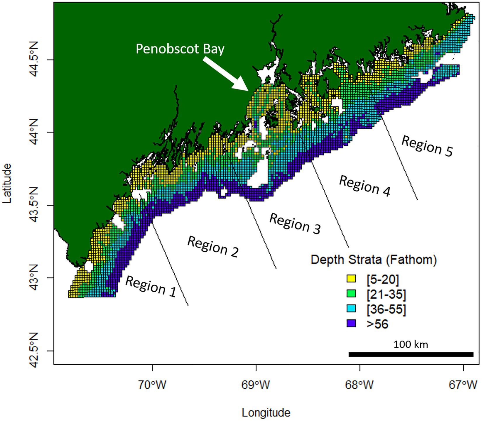
Figure 1. Maine-New Hampshire Inshore Bottom Trawl Survey regions and depth strata. This survey is subdivided into five regions which include (1) New Hampshire and Southern Maine, (2) Mid-Coast Maine, (3) Penobscot Bay, (4) Mt. Desert Island, and (5) Downeast Maine. Missing white areas within the 12-mile survey grid area are non-surveyable locations due to the topography of the ocean floor at those locations.
The survey area extends 12 nautical miles (22.22 km) offshore and is broken up into 4 different depth strata (Figure 1). A target of 115 stations is set for each survey, creating a sampling density of roughly one station for every 40 NM2 (137.20 km2). Random stations in this survey are chosen by dividing the survey area into a 1 NM2 (3.43 km2) grid, where cells are chosen at random using an Excel random number generator (Sherman et al., 2005). Each survey aims for a target tow of 20 min at a speed of 2.2–2.3 knots (4.1–4.3 km/h), which covers approximately 0.8 NM (1.48 km, Sherman et al., 2005). Data from 486,971 individual lobsters were included in this study. See Supplementary Figures 1, 2 for mean catch trends in the bottom trawl survey data by region.
This study utilizes data from the 2000–2019 bottom trawl surveys. Biological data taken on each lobster include carapace length (mm), sex, presence of eggs or v-notches, and if any noticeable damage is present. Lobsters are then sorted into baskets by sex and baskets are weighed once filled (Sherman et al., 2005). Data have been standardized to 20-min tows to ensure all catch, weight, and length frequency information is comparable. In addition to biological data, bottom water salinity, bottom water temperature, and depth data were collected during each tow by using a Sea-Bird ElectronicsTM 19plus SEACAT profiler, which was attached to the starboard door wire, turned on and lowered overboard (Sherman et al., 2005). Bottom trawl survey bottom temperature and bottom salinity data were recorded at a single point along each tow transect and do not represent an average across each tow length, The net used for this survey is a type of modified shrimp net that is used for “near-bottom dwelling species,” although not intended for any single species in particular (Sherman et al., 2005). More information about the Maine-New Hampshire Inshore Bottom Trawl survey procedures, protocols, or specifics can be found in Sherman et al. (2005). This survey has been found to yield informative data for studying lobster distributions and habitats in the GOM (Tanaka and Chen, 2016; Tanaka et al., 2019; Hodgdon et al., 2020).
Bottom water temperature, bottom water salinity, average depth, latitude, and longitude information from each tow were used from the bottom trawl survey to inform the models. Distance from shore and median sediment size were also estimated and included in the models. Distance from shore was estimated using the “distances” function from the package “distances” (Savje, 2019) in R, which finds the shortest distance between points, in this case, the distance between the midpoint latitude and longitude of a tow and the closest point on the coast. Sediment data were sourced from the East Coast Sediment Texture Database which is run by the United States Geological Survey (U.S. Geological Survey, 2014). This survey was last updated in 2014 and contains information such as location, description, texture, and size (phi, −log of grain size) taken by different marine sampling programs across various locations around the world. Both mean and median sediment size values are supplied in this dataset, but median sediment size was used over mean sediment size, as the former is more robust to outliers (Tůmová et al., 2019). The median grain size at each survey location was estimated using thin plate splines. These data can be found at https://woodshole.er.usgs.gov/openfile/of2005-1001/htmldocs/datacatalog.htm and more information about the East Coast Sediment Texture Database can be found in U.S. Geological Survey (2014).
Although models were built using bottom trawl survey bottom temperature and bottom salinity data, additional bottom temperature and bottom salinity data were needed to create interpolated distribution plots. These additional data were not used to inform the models, but rather served as data that the models used to be able to estimate lobster density at unsampled locations. Thus, bottom temperature and bottom salinity data throughout the study area were obtained by spatially interpolating Finite-Volume Community Ocean Model (FVCOM) data. The FVCOM is an advanced ocean circulation model that uses an unstructured grid format, making it highly applicable for use in regions with complex coastlines and bathymetry (Chen et al., 2006; Li et al., 2017). The FVCOM was developed by University of Massachusetts Dartmouth and Woods Hole Oceanographic Institution. More information about the FVCOM can be found in Chen et al. (2006).
Forecasted distributions were made for the period 2028–2055. The forecasted bottom temperature and bottom salinity data were sourced from the National Oceanic and Atmospheric Administration (NOAA) and represent an ensemble projection of all models used to create the Intergovernmental Panel on Climate Change’s (IPCC) Coupled Model Intercomparison Project Phase 5 (CMIP5) data (NOAA Physical Science Laboratory, n.d.). Data for the Representative Concentration Pathway (RCP) 8.5 “business as usual” scenario were used. These data are forecasted anomalies based on the reference time period 1956–2005 and are estimated for the period 2006–2055. These data are anomalies, and thus hindcasted bottom temperature and bottom salinity data must be used in tandem from the same reference period. The anomalies were added to the corresponding reference period FVCOM data. However, the earliest available FVCOM data begins in 1978 rather than 1956, limiting the available reference period in this study to 1978–2005. With the reference period reduced from 50 to 27 years, the CMIP5 forecasting period must also be reduced, respectively, from the initial 2006–2055 to 2028–2055 for this study. The forecasting period 2028–2055 is used because it represents the maximum amount of FVCOM data than can be used while also confidently applying IPCC forecasted anomalies. Delta downscaling methods were also applied so that forecasted anomalies could be applied to the same scale as the FVCOM data. Specifically, bivariate spline interpolation was applied using the package “akima” in R (Akima and Gebhardt, 2016).
Model Development
Lobster densities were standardized per tow and divided into eight groups based on season (fall and spring), sex (female and male), and size (adult and juvenile; Li et al., 2018; Chang et al., 2010). Juvenile lobsters were distinguished as lobsters with carapace lengths <50 mm due to differences in activity patterns (Lawton and Lavalli, 1995). Each of the eight groups were modeled independently under three different techniques: (1) a GAM that assumes stationary relationships between species distributions and environmental variables (GOM–GAM); (2) a GAM that assumes nonstationary relationships between eastern and western GOM (West-GAM, East1-GAM), and (3) a GAM that assumes nonstationary relationships between eastern, central, and western GOM (West-GAM, Central-GAM, and East2-GAM). Partitioning of data for these models can be visualized in Figure 2.
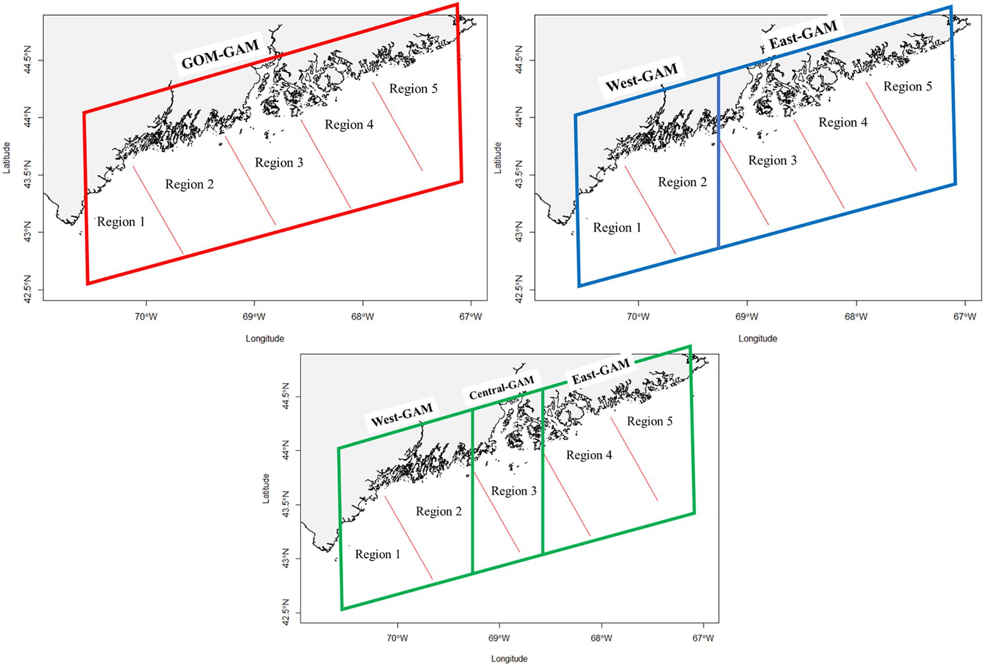
Figure 2. Visual representation of each model utilized in this study. Each colored quadrilateral represents a separate GAM that was ran on the observed data points contained within that area. Red lines designate bottom trawl survey regional boundaries.
Previous literature in the GOM have estimated species distributions using stationary models at a large spatial scale (Chang et al., 2010; Becker et al., 2020). This technique is represented in this study by the “GOM–GAM” model, which assumes no nonstationarity and is applied at the largest spatial scale. This technique also assumes that nonlinear (but stationary) relationships between lobster density and environmental factors are sufficient to accurately predict a species spatial distribution across an ecologically complex region. Other literature has highlighted differences in environment-abundance relationships between localized regions (Li et al., 2018; Liu et al., 2019). Thus, the bisected (comprized of West-GAM and East1-GAM) and trisected (comprized of West-GAM, Central-GAM, and East2-GAM) models were constructed at smaller spatial scales to capture evidence of these differences. The purpose of this study is to explore how spatial distribution predictions change under models with varying assumptions of nonstationarity (or lack thereof) in hindcasting and forecasting scenarios.
The first set of localized models (West-GAM and East1-GAM) broke up the data into east and west zones. The West-GAM used data that were west of −69.27457 degrees longitude. The East1-GAM was represented by data east of −69.27457 degrees longitude. The decision to split the data up along the −69.27457 degree longitude line was in part because regions one and two of the bottom trawl survey are west of the Penobscot Bay region and −69.27457 is the approximate longitudinal line where region two of the bottom trawl survey intersects the coastline. This decision was also driven by the GOM coastal currents and the supporting literature that states the southern extent of the EMCC includes the Penobscot Bay region (Xue et al., 2008; Chang et al., 2016).
Although some literature supports this decision, it is difficult to exactly pinpoint a fine line of where the EMCC diverges and the WMCC begins. Thus, another argument can be made in which the Penobscot Bay area (≅region three in the bottom trawl survey) could act as a potential buffer zone, in which this area of possible mixing between currents could throw off GAM relationship curves if the this area were to be included into a particular side. One previous study used a similar trisected approach to view relationships between initial intra-annual molts of American lobster and bottom temperatures in the GOM (Staples et al., 2019). Consequently, the second set of localized models (West-GAM, Central-GAM, and East2-GAM) are built in in such a way that the West-GAM is the same in spatial area and extent as previously described, but the Central-GAM is comprised of data between −69.27457 and −68.58246 degrees longitude, and the East2-GAM is comprised of data east of −68.58246 degrees longitude.
Prior to model construction, covariance matrices and variance inflation factor (VIF) tests were run to check for variable independence and multicollinearity. Running multiple covariance metrics showed a high dependence between distance from shore and average depth variables. Distance from shore was kept over average depth because distance from shore had a lower covariance value amongst the rest of the variables than average depth. VIFs quantify the multicollinearity amongst variables. Variables with VIF numbers >3 were excluded from the model (Zuur et al., 2009), supporting the decision to remove average depth as a variable when building the models. The following variables were shown to be significant in every GAM: latitude and longitude combined as an interaction term, and bottom temperature. Bottom salinity, distance from shore, and sediment size were found to be significant in some models, but not all. Significant variables and deviance explained for each group are summarized in Tables 1, 2, respectively.
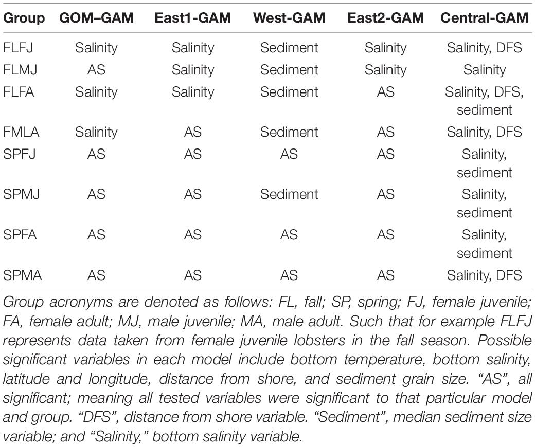
Table 1. Non-Significant variables for each model and group type.
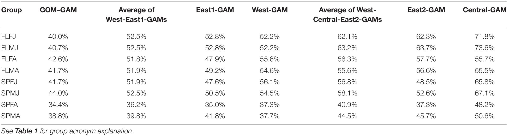
Table 2. Deviance explained for each model and group type.
Generalized Additive Models were used to evaluate the relationships between lobster abundance and environmental variables. A GAM is an extension of a generalized linear model, with a smoothing function added. GAMs follow the assumptions that the functions are additive, and the components of the functions are smooth (Guisan et al., 2002). A separate GAM was created for each group of lobsters that differs in season, sex, and size, based on the assumption that males, females, juveniles, and adults will all respond to environmental variables differently, and that seasons will also impact the relationships with the environment differently. We used a tweedie GAM to estimate lobster abundance (y). GAMs were built using a backward fitting technique based on covariate significance (p < 0.05; Chang et al., 2010). A GAM using all potential environmental variables can be written as:
where s is a spline smoother, La, Lo is an interaction term between latitude and longitude, Bt is bottom temperature (°C), BS is bottom salinity (PSU), DFS is distance from shore (decimal degrees), and Ss is median sediment size (phi).
Hindcasted distribution plots were created for each lobster season × sex × size group and for each model approach for the years 2000, 2006, 2012, and 2017 for a total of 96 plots. Although there are bottom trawl survey data available from 2000–2019 to inform the models, environmental FVCOM data used for interpolation are only available until 2017, limiting the most recent available hindcasting year that can be spatially interpolated to 2017. Additionally, these years were chosen because they are roughly evenly spaced throughout the hindcast period of interest, albeit these methods could be applied to any year(s) 2000–2017. Forecast distribution plots were also estimated for the 2028–2055 years period, for a total of 24 forecast distribution plots (eight lobster groups ×3 model approaches). Model fitting was accomplished by using all survey data between the years 2000–2019 and predictions were estimated for each tested year (2000, 2006, 2012, 2017, and the forecast period 2028–2055) separately, by using the corresponding annual FVCOM data. Differences between GOM–GAM and localized approaches were determined by calculating relative differences between density distribution estimates. Relative differences were estimated using the equation
where i is a location within the study area and “localized” represents the estimated lobster density at location i from a localized model (West-GAM, East2-GAM, etc.). Relative difference plots were generated for each lobster season × sex × size group and for the same years as the hindcast and forecast distribution plots. These plots demonstrate the magnitude and location of where the GOM–GAM models tend to over or under predict abundances in relation to the localized approaches. All distribution and relative difference plots were interpolated using bivariate splines using the package “akima” in R in order to achieve high resolution smooth distributions (Akima and Gebhardt, 2016).
Model Fitting and Validation
Root Mean Square Error (RMSE), Akaike Information Criterion (AIC), and Moran’s I were used to access model fit for all models. RMSE measures the differences between predicted and observed values where values closer to zero represent better model fit (Stow et al., 2009). AIC is another method to test goodness of fit and model complexity with a model having smaller returned AIC value being the better model (Zuur et al., 2009). Moran’s I tests for spatial autocorrelation in residuals where a significant Moran’s I of −1 signifies perfect clustering of dissimilar values, a significant Moran’s I value of 0 signifies no autocorrelation, and a significant Moran’s I of +1 signifies perfect clustering of similar values. If values are found to be spatially autocorrelated, this is an issue as it violates the assumption of independence of data (Zuur et al., 2009; Stephanie, 2016). Additionally, two-fold cross validation was performed by separating each of the eight groups’ (2 season × 2 sexes × 2 sizes) data into random training and a testing subset to calibrate the model and validate its predictions (Li et al., 2018). The percentage of data allocated for the testing portion was determined by the equation
where P is the number of predictor variables (Franklin, 2010; Li et al., 2018). Cross validation allows visualization of model performance to examine if model predictions are on average, over or under predicting abundance compared to observed values. 100 iterations of cross validation were repeated for each model group and average performance was estimated.
Results
Model Performance and Validation
Significant variables differed between model types and between groups. Under the GOM–GAM, only salinity was found to be non-significant in some groups, whereas both salinity and sediment size were found to be non-significant in some West-GAM and East1-GAM groups. Moreover, salinity, sediment, and distance from shore were found to be non-significant in some West-GAM, Central-GAM, and East2-GAM groups. Table 1 summarizes the non-significant variables which were not included in the final model for each group and spatial scale. The deviance explained for lobster abundance varied between 34.4 and 44.0% for each group of the GOM–GAM, 36.2–52.5% for the average West-GAM and East1-GAM group, and 40.9–63.2% for the average West-GAM, Central-GAM, and East2-GAM group. Full deviance explained for each specific group can be found in Table 2. Likewise, the RMSE, AIC and Moran’s I tests showed similar trends in model fit, with the GOM–GAM demonstrating the lowest model fit estimates, the West- and East1-GAM approach demonstrating intermediate model fits, and the West-, Central-, and East2-GAM approach demonstrating the greatest model fits (Table 3).
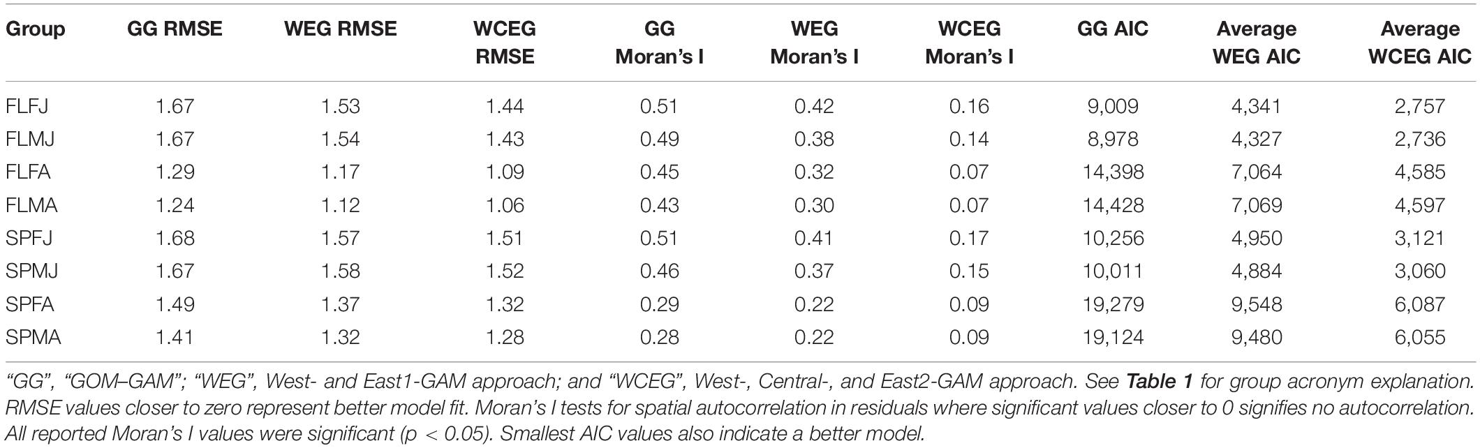
Table 3. RMSE, Moran’s I, and AIC values for each model and group type.
The two-fold cross validation results from 100 iterations revealed that the models had reasonable prediction skill, as the average between the 100 iterations was near the 1:1 prediction line for most groups and models. These tests revealed that most models tended to slightly underpredict abundance, with exception of the average spring female adult (SPFA) West- and East1-GAM approach which revealed average slight overpredictions. The West-, Central-, and East2-GAM approach cross validation results demonstrated more precision than West- and East1-GAM or GOM–GAM results. Results from the two-fold cross validation can be found in the Supplementary Material section (Supplementary Figures 1–3).
Environmental and Spatial Variables
Environmental and spatial variables were also explored via GAM response curves for each significant predictor variable. Latitude and longitude variables were combined as an interaction term in each model to help account for spatial autocorrelation (Siegel and Volk, 2019). Response curves varied greatly depending on independent variable, season, sex, size, and spatial scale of the model. For bottom temperature, highest partial effect on abundance was seen between 6 and 10°C in the spring and around 10–14°C in the fall for GOM–GAMs, and between 4 and 10°C in the spring and 10–14°C in the fall for the localized model approaches. For bottom salinity, highest abundance was seen between 31 and 33 psu for both spring and fall across all models. The relationship spring male adult (SPMA), spring female juvenile (SPFJ), and spring male juvenile (SPMJ) groups had with salinity was unique, compared to other groups. These group’s response curves demonstrated a higher partial effect on abundance at salinity levels >32 psu in the west. This may help explain the distinctive relative difference trends generally observed in western GOM for the SPMA group. This difference did not seem to affect the spring juvenile groups, as juvenile lobster tend to stay in more nearshore waters (Lawton and Lavalli, 1995), where FVCOM data has shown salinity levels are generally lower in western GOM. For distance offshore, highest partial effect on abundance was seen generally between 0.00 and 0.1 decimal degrees (≅0–6 nautical miles offshore), and then gradually declined with increasing distance from shore across most models. For sediment size, highest partial effect on abundance was seen between 2 and 6 phi (silt – medium grain sand) across most models. Some season, sex, and size group curves changed more in shape across spatial extents than others, but variation was apparent and supports evidence of spatial nonstationarity in this region. Figure 3 depicts the response curves between lobster abundance and bottom temperature for SPMAs (Figures 3A,B) and fall female juveniles (Figures 3C,D). These figures show how the response curves change, depending on the spatial scale and location of the testing data. These figure panels also show where estimated relationship curves overlap, if at all. For example, in Figure 3B, one can see high overlap between most model response curves between 5 and 7°C. However, at temperatures greater than 7°C, the relationship curve for the GOM–GAM more closely resembles that of the response curve for the East2-GAM than for the West- or Central-GAM. This suggests that if a large-scale model were used to represent SPMA lobster data, it would better represent eastern GOM data than central or western GOM data in that temperature range, and in a climate warming scenario, would underestimate western GOM abundances. In a region which is expected to continue experiencing warming temperatures, the implications of subordinate model spatial scale selection may increase. Many lobster groupings (season × sex × size) tended to show similar patterns, where the GOM–GAM response curve for a variable, more closely resembled the response curve of one localized region of the GOM more than the other regions.
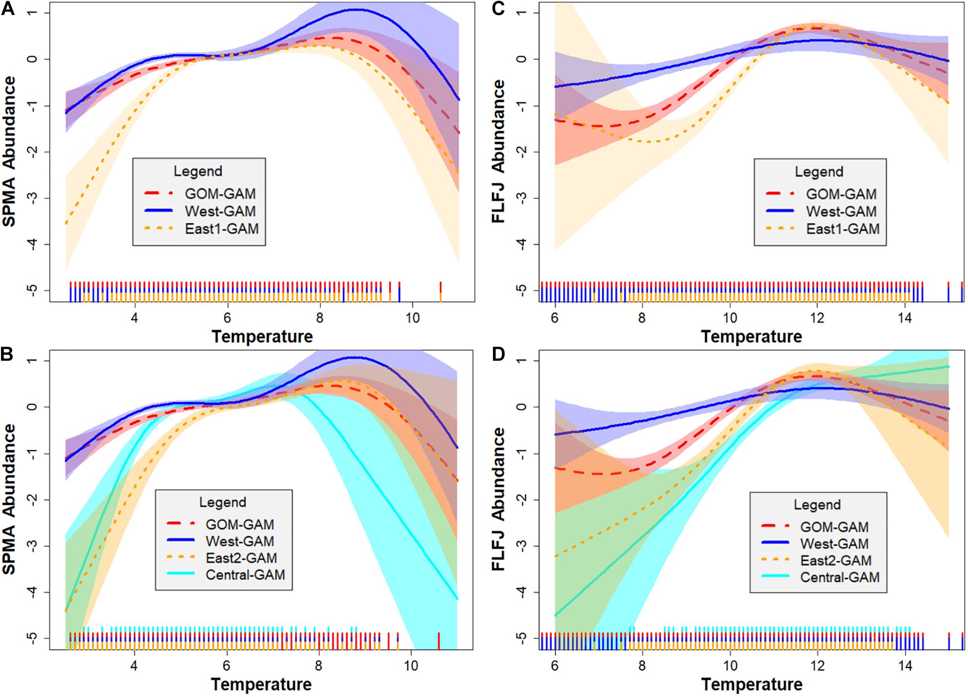
Figure 3. A comparison of spring male adult (SPMA) and fall female juvenile (FLFJ) lobster GAM bottom temperature response curves by spatial location in the GOM. Each plot shows the response curve of bottom temperature (°C) on the x-axis, against the partial effect of lobster density on the y-axis. Figures (A,C) compare response curves estimated for the GOM–GAM, West-GAM, and East1-GAM, while figures (B,D) compare response curves estimated for the GOM–GAM, West-GAM, Central-GAM, and East2-GAM. Shaded regions on either side of the response curve line indicate the standard error confidence intervals. Rug plot lines along the x-axis of each plot indicate distribution of the bottom temperature data. These response curves were estimated using 2000–2019 ME-NH Inshore Bottom Trawl survey data and are applicable to all years tested.
Model Prediction and Distribution Plots
Fall distribution plots showed greater abundance estimates than spring plots, which correlates with observations in raw trawl survey data. Raw fall trawl survey trends show slight declines in catch in regions three and four since 2015 and in region five since 2016 (Supplementary Figure 4), with trends of offshore catch increasing overtime. All three model estimates demonstrated offshore abundance estimates increasing from the 2012–2017 hindcasts, but only the East2-GAM showed indications of a slight decrease in eastern GOM abundance. Model estimates in central GOM were most distinctive between models. A trend emerged in all tested years which demonstrated that as model spatial scale became finer, clear “hot” and “cold” spots emerged within the Penobscot Bay area. The Central-GAM showed this pattern well, with a “hotspot” emerging along the southwest mouth of Penobscot Bay, and a “coldspot” in the northeast Penobscot Bay region (Figures 4–7). These patterns correlate well with American lobster settlement patterns found in Steneck and Wilson (2001).
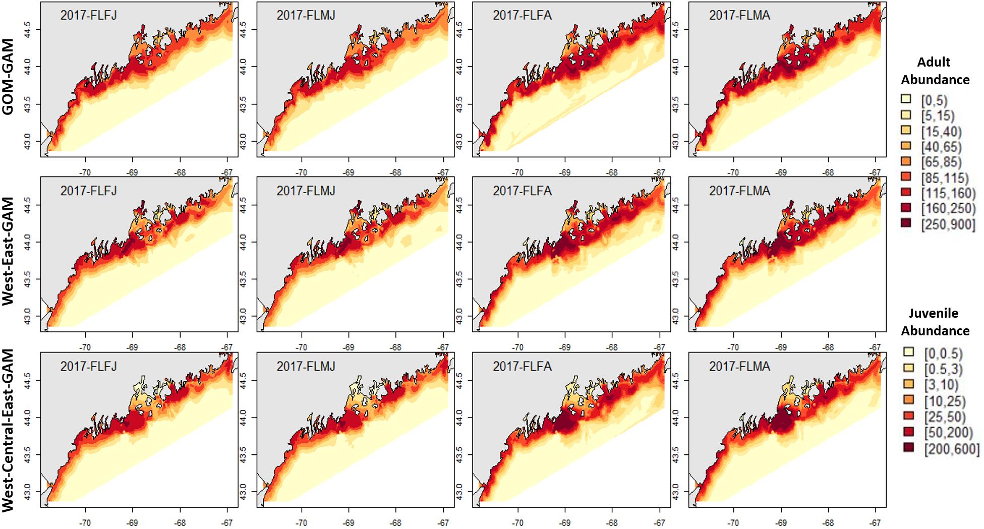
Figure 4. 2017 Fall American lobster estimated spatial distribution. Legend colors increase in abundance estimates from pale yellow to dark red. Each column represents a season × sex × size group. Each row represents the modeling approach used to generate the abundance estimations. Adult abundance legend corresponds with adult lobster group estimates. Juvenile abundance legend corresponds with juvenile lobster group estimates.
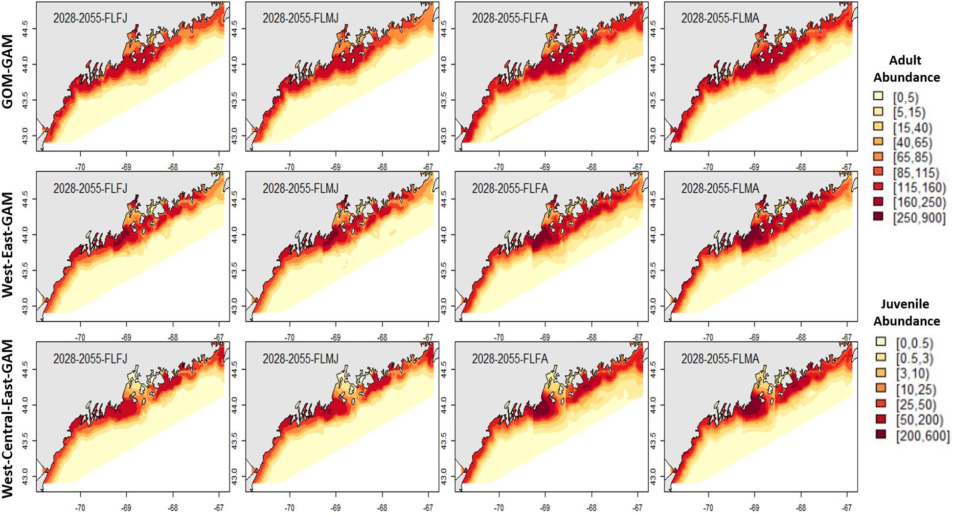
Figure 5. Forecasted fall American lobster estimated spatial distribution for the time period 2028–2055. See Figure 4 for figure details.
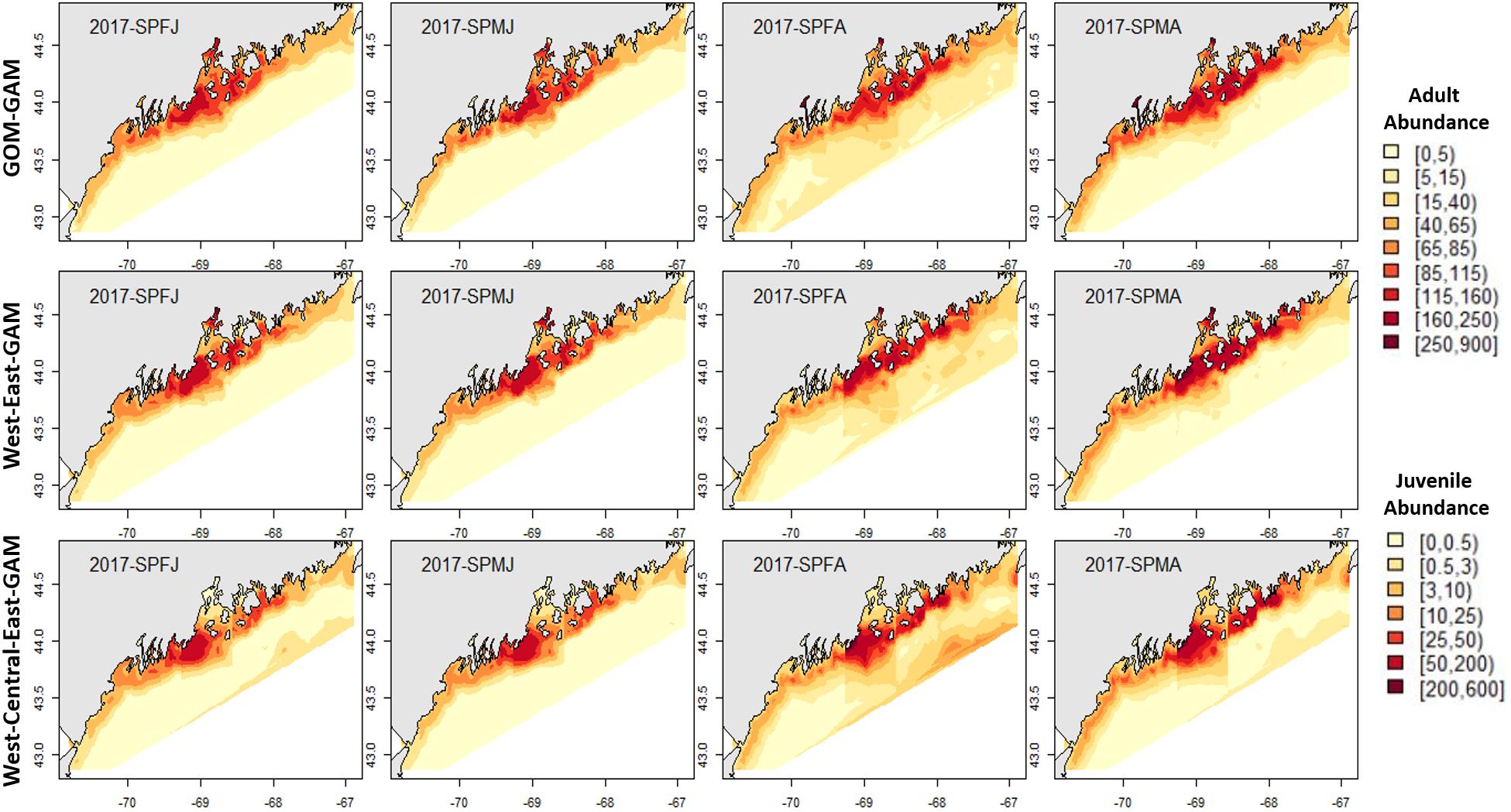
Figure 6. 2017 spring American lobster estimated spatial distribution. See Figure 4 for figure details.
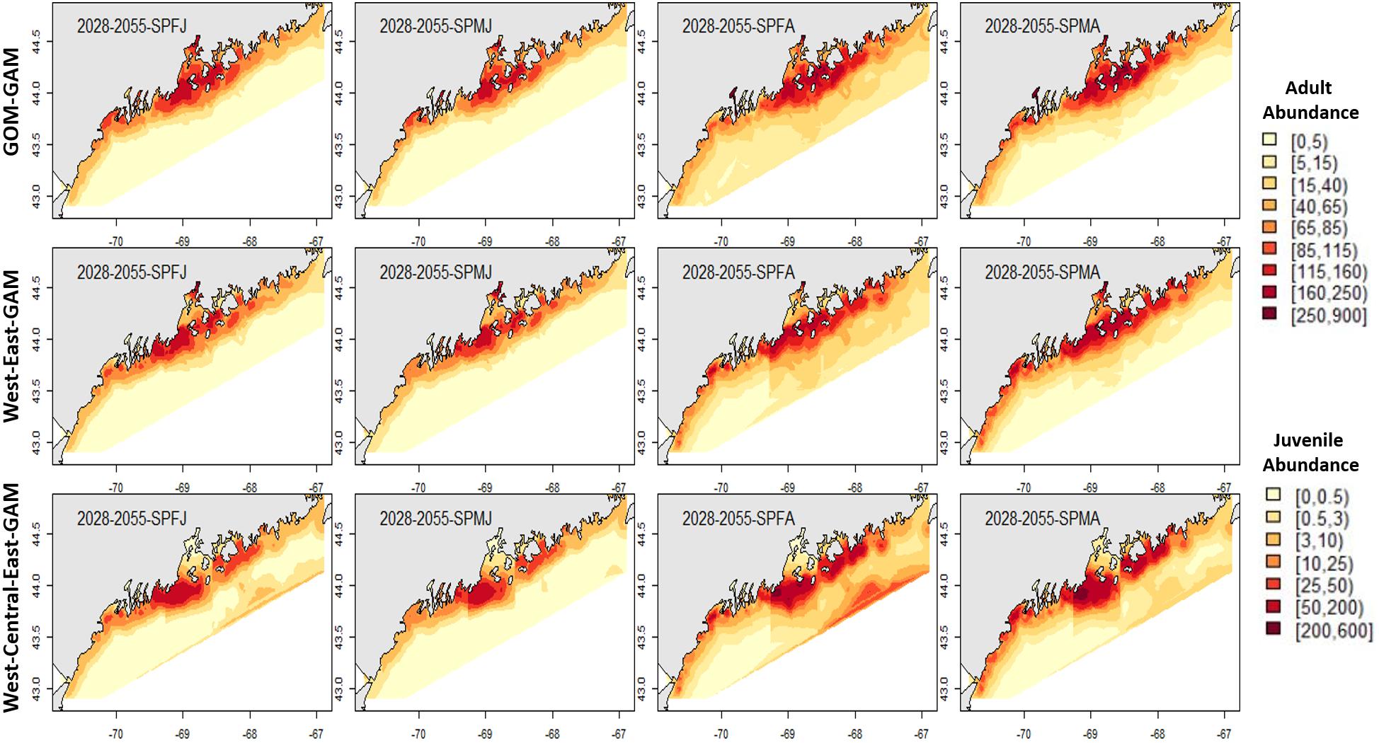
Figure 7. Forecasted spring American lobster estimated spatial distribution for the time period 2028–2055. See Figure 4 for figure details.
The GOM–GAM tended to overpredict the 2017 hindcast distributions in western GOM, apart from the SPMA group (Figure 8). In central GOM, the GOM–GAM models tended to comparatively underpredict in the western part of Penobscot Bay and overpredict in the eastern part of Penobscot Bay. This was evident across all years in both relative difference comparisons when the GOM–GAM estimates were compared to the West- and East1-GAM approach, as well as in the West-, Central-, and East2-GAM approach (Figure 8). In eastern GOM, many GOM–GAMs estimated less abundance approximately between −68.5° and −67.5° W, and higher abundance estimates between −67.5° and −67° W when compared to West- and East1-GAM approaches (Figures 8, 9). These trends were present across all tested years.
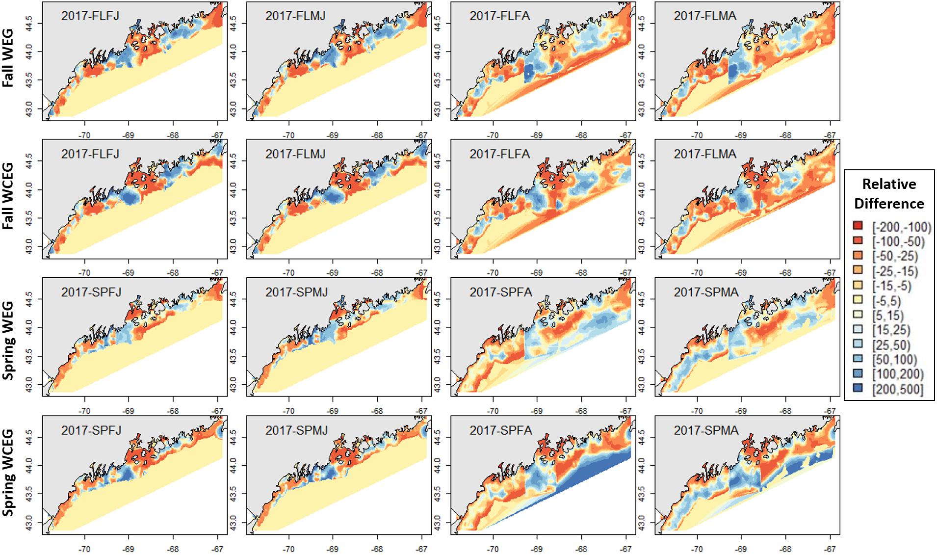
Figure 8. 2017 American lobster relative differences in model abundance estimates. Legend numbers represent relative differences (%) between either the West-East1-GAM (WEG) or the West-Central-East2-GAM (WCEG) approach and the GOM–GAM. Red legend colors indicate areas where the GOM–GAM is predicting higher lobster abundance than the model in comparison. Blue legend colors indicate areas where the GOM–GAM is predicting lower lobster abundance then the localized model approach in comparison. Pale yellow colors indicate similar abundance estimates between the GOM–GAM and localized models. Each column represents a lobster season × sex × size group. Each row represents the season and localized model approach compared to the corresponding GOM–GAM.
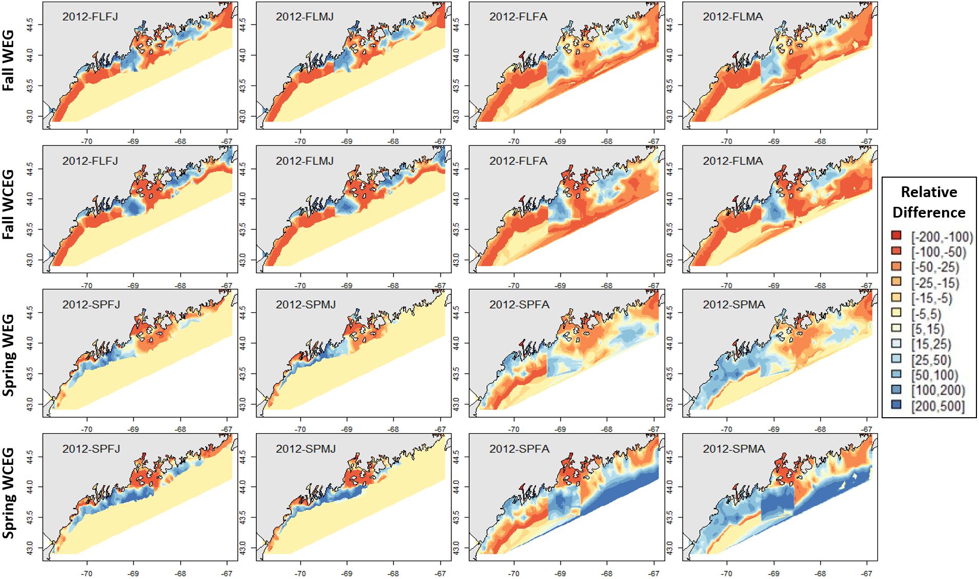
Figure 9. 2012 American lobster relative differences in model abundance estimates. See Figure 8 for figure details.
Estimates for the 2028–2055 period from localized and large-scale approaches exemplify similar spatial patterns seen in the corresponding distributions from 2000 to 2017. Some season × sex × size groups estimated abundances that extend further offshore than their hindcast counterparts (see Figures 4–7). Spring abundance estimates demonstrate an increase in central and eastern GOM from 2017 to 2028–2055, although this is more notable in the localized models than the GOM–GAMs (see Figures 6, 7). These forecasted estimates correlate with raw spring bottom trawl survey data thus far for regions 3–5, which have all demonstrated general increasing average catch rates (number/tow) from 2000–2019 (Supplementary Figure 5).
In general, relative differences between the GOM–GAM and the West-Central-East2-GAM approach resulted in larger differences when compared to the relative differences between the GOM–GAM and the West-East1-GAM approach. This trend was apparent across all tested years. These observations correlate with observations in model fit, as the West-Central-East2-GAM approach showed highest model fits, and the West-East1-GAM approach showed model fits more similar to that of the GOM–GAMs. Fall relative difference plots revealed that the GOM–GAMs were likely to estimate higher abundance in western GOM when compared to the West-GAM (Figure 10). In the spring, the GOM–GAM comparatively estimated lower abundance in western GOM for spring adult males in the 2028–2055 period (Figure 10). For adult females in both fall and spring, however, GOM–GAMs estimated higher abundance in western GOM than the West-GAMs did in that same region for the 2028–2055 period (Figure 10). Forecasted GOM–GAM abundance plots estimated lower abundance in the western portion of central GOM (≈−69.3 to −68.9° W) and estimated higher abundance in the eastern portion of central GOM (≈−68.9 to −68.1° W), when compared with distribution estimates derived from the East1-GAM in that same area (Figure 10). This trend was also apparent in GOM–GAM and Central-GAM forecasted relative difference plots, but differences were slightly more polarized. There were slightly less consistent and patchy trends in relative differences amongst groups in eastern GOM for the 2028–2055 forecasted period, where both higher and lower estimates were evident (Figure 10).
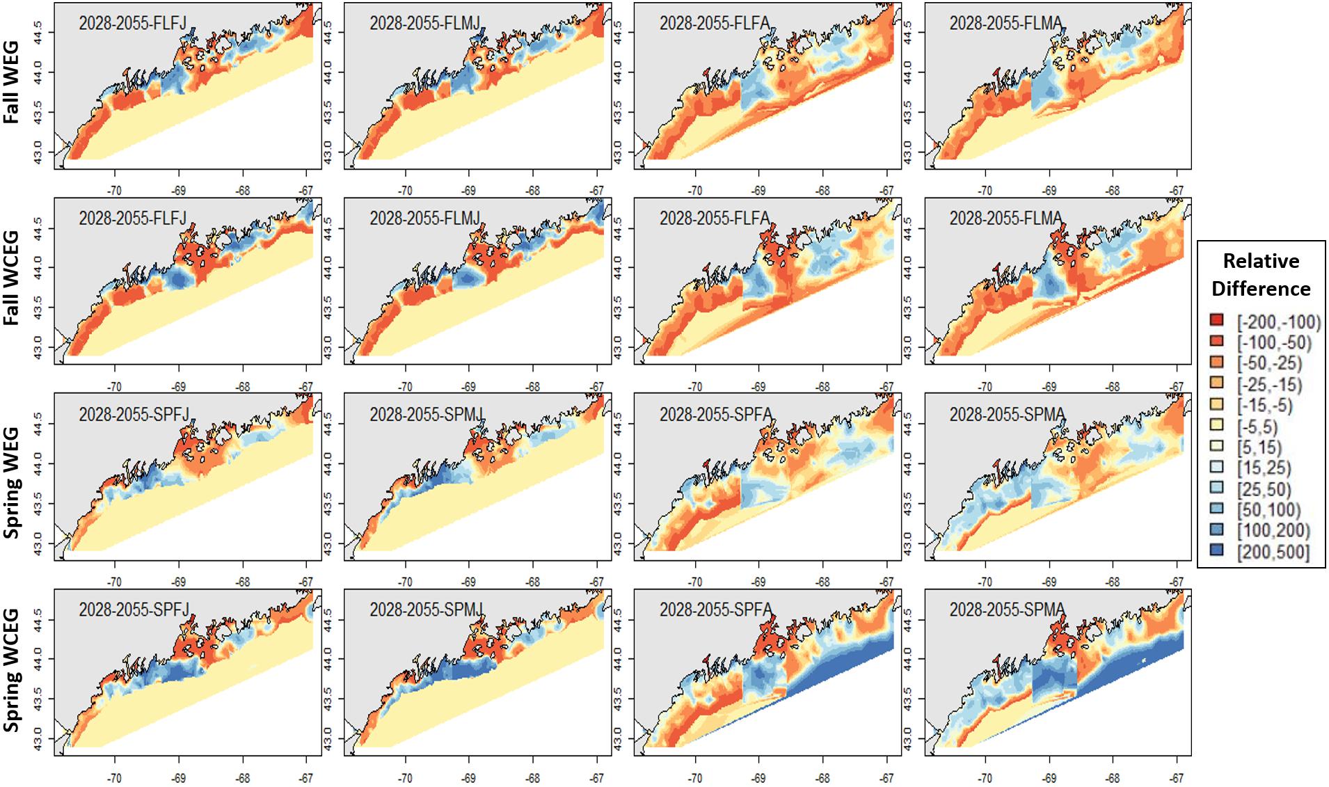
Figure 10. Forecasted American lobster relative differences in model abundance estimates for the period 2028–2055. Legend numbers represent relative differences (%) between the West-East1-GAM (WEG) approach or the West-Central-East2-GAM (WCEG) approach and the GOM–GAM. Red legend colors indicate areas where the GOM–GAM model is predicting higher lobster abundance than the localized model approach in comparison. Blue legend colors indicate areas where the GOM–GAM model is predicting lower lobster abundance then the localized model approach in comparison. Pale yellow colors indicate similar abundance estimates between the large-scale and localized models. Each column represents a lobster season × sex × size group. Each row represents the season and model type compared to the corresponding GOM–GAM.
Discussion
We developed a modeling approach to explore and demonstrate how estimates of season-, sex-, and size- specific American lobster spatial distribution and abundance would vary based on the spatial scale and extent of the area being modeled in the GOM. Validation tests run for each model type and season × sex × size group suggested reasonable predictive ability. Nonsignificant variables varied by model and spatial location. These results correspond with the notion that local patterns may get masked by global statistics, if stationary assumptions are made (Brunsdon et al., 1996; Windle et al., 2012). Stationary assumptions are likely to be violated in the GOM, where northeast to southwest gradients of bottom water temperature, salinity, and productivity have been observed (Lynch et al., 1997; Pettigrew et al., 1998; Chang et al., 2016), as well as spatial differences in American lobster stock-recruitment relationships (Chang et al., 2016), and spatially varying patterns in initial molt timing and suddenness (Staples et al., 2019).
A trend in model fit was observed in which as the spatial scale of models became more localized, model fit increased. The West-Central-East2-GAM approach demonstrated the greatest model fit to the bottom trawl survey data and showed the most correlation in abundance estimates with raw bottom trawl survey data, indicating greater distribution estimation capabilities. The West-East1-GAM approach demonstrated the next highest model fit and estimation capabilities, while the GOM–GAM model demonstrated the lowest model fit to the data. We speculate that the West-Central-East2-GAM approach shows the greatest model fit and potential predictive capabilities because of the modeling technique used on these data. By taking into consideration the oceanographic processes in the GOM to determine which localized areas are likely to be the most and least similar in relationships between American lobster abundance and environmental variables, the amount of data used for model estimation can be maximized, while limitations of large-scale models over a biologically complex region can be minimized. Out of the localized scale model approaches, the results of West-Central-East2-GAM approach suggest an improvement upon the West-East1-GAM approach. Although these approaches are similar, the evidence of the West-Central-East2-GAM approach being an improvement upon the West-East1-GAM approach suggests that enough nonstationary exists between central and eastern GOM to make the tripartite model subdivision worthwhile and that this technique may be more biologically reflective. Spatial distribution estimates of the West-Central-East2-GAM approach also seem to correlate well with raw bottom trawl survey data and past literature, especially in central GOM which has shown high increases in average catch over the course of the survey, and where localized “hot” and “cold” spots may be reflective of lobster settlement patterns observed in that region (Steneck and Wilson, 2001).
Most lobster groups demonstrated similar spatial patterns or temporal trends in model results and analysis, with the frequent exception of SPMA groups. We speculate the SPMA lobster groups often did not respond in the same way due to differences in both bottom temperature and bottom salinity response curves. Although each group had more than one significant environmental variable across model techniques, bottom temperature was a significant variable in all models, and spring adult (male and female) bottom temperature response curves were most distinct among groups. Most other season × sex × size groups displayed a relationship with bottom temperature was similar to that of the FLFJ group (Figure 3D), where the partial effect of bottom temperature on abundance generally increased then plateaued with increasing temperature. Spring adult lobster often did not follow this pattern, as exemplified in Figure 3C, where spring adult curves were typically domed-shaped. This dome-shaped pattern was present in both female and male spring adult groups, however, so it is likely that other influences, such as salinity, may be a potential factor. The relationship spring adult males had with salinity was unique, compared to spring adult females, which demonstrated a similar pattern to the other season, sex, and size groups. The spring adult male group response curve demonstrated a higher partial effect on abundance at salinity levels >32 psu in the west, which may explain why the GOM–GAMs were more likely to comparatively underestimate lobster abundance in that region.
The West-Central-East2-GAM approach demonstrated the greatest relative differences across all years when comparing its spatial abundance predictions to those of the GOM–GAM. This observation is the result of the multiple unique GAMs run on localized data, and thus assumptions of spatial nonstationarity are better satisfied. However, it is important to recognize that the largest difference from the GOM–GAM does not automatically equate to the best model, as it is difficult to determine the starting biological accuracy of the GOM–GAM. Results from the three modeling techniques at bottom trawl survey locations could be compared to raw bottom trawl data at those same locations to get a better understanding of how biologically accurate each technique is at producing estimates. However, between evidence of model fit and validation, distribution plot results, and correlation with raw survey data, we conclude that applying model techniques that better account for spatial nonstationarity will result in increased model performance.
While the West-Central-East2-GAM approach demonstrated the best model fit out of the tested models, it is important to acknowledge some of the limitations of this model and the techniques used. First, all models tested only included environmental variables. No biological variables were included in the models; thus, these models are working under the assumption that lobster abundance is dependent solely upon environmental variables and spatial scale. Future studies may benefit from including biological variables, such as predator and/or prey abundance, into the models to see how the results would differ. Secondly, the subdivision of data technique used for the localized models (West-East1 and West-Central-East2 GAMs) sometimes resulted in variegated or “patchwork” spatial distribution estimates. Such abrupt changes in abundance estimates along the model extent lines are not likely to be biologically representative of true American lobster spatial distributions in the GOM. Consequently, this piecewise, localized modeling approach should only be used to observe trends in spatial distribution estimates, and not for precise estimations of “true” abundance, especially near the model extent lines. Thirdly, future studies may also benefit from exploring how different ways of subdividing data can impact model results, and if model fit can be further improved with more data partitions. Lastly, it is likely that the relationships explored in this study do not only vary across space, but over time as well. This study only considers spatial nonstationarity in model development, as gradients in environmental conditions throughout the study area have been observed. We did not consider temporal autocorrelation in this study. Based on the results from this study, it is likely that accounting for temporal autocorrelation could impact species distribution results as well and that excluding temporal autocorrelation may have introduced biases into the forecasts. However, this is beyond the scope of this study.
This study indicates that SDM estimations are dependent upon spatial scale and assumptions of nonstationarity. Results from a model that implicitly assumes spatial stationarity would differ from results of a model that better accounts for spatial nonstationary processes. Thus, using results generated by large-scale, stationary models could lead to different, or potentially even ill-informed management decisions which may result in less effective management results. Moreover, accounting for localized processes may be essential when devising localized regulations, as indications of change or unique dependencies of a species may be masked when using global statistics. Management decisions informed by large-scale, stationary models could result in regulations being more effective in one local area and less in others, if the relationship curves that drive the predictions are more representative of a particular area of the study area, rather than well represented throughout. If the West-Central-East2-GAM model distribution estimates are more biologically realistic as the analyses suggest, then comparatively, under an RCP 8.5 “business as usual” climate scenario prediction for the years 2028–2055, large-scale, stationary models could overestimate lobster abundances in western GOM, with the exception of spring adult males. In such case, it is important local heterogeneity is considered in American lobster management in the GOM because false overestimations of abundance could lead to relaxed regulations or ill-informed biological reference point calculations, which could potentially lead to overfishing in western GOM.
Using large-scale, stationary modeling techniques to forecast American lobster spatial distribution could result in subordinate perceptions of where lobster populations will be spatially, and to what extent. More accurate predictions of American lobster spatial distributions will help stakeholders prepare and employ best practice measures to ensure the sustainability and longevity of the industry.
Data Availability Statement
The data analyzed in this study is subject to the following licenses/restrictions: Multiple datasets were utilized in this study. Most are publicly available, but the ME-NH Inshore Bottom Trawl Survey Data are not. Publicly available data have been compiled and can be found at https://github.com/Jamie-Behan/Nonstationary-Effects-on-Spatial-Distribution.git. Requests to access these datasets should be directed to Jamie Behan, amFtaWUuYmVoYW5AbWFpbmUuZWR1.
Author Contributions
YC drafted the project conception. BL supplied some foundational code. JB substantially contributed to the finalized code which was used. JB accomplished interpretation of data, with support from BL and YC. JB completed the manuscript drafting, with manuscript revisions by BL and YC. All authors drafted the project design, and approve the submitted manuscript.
Funding
This work was funded by the Maine Department of Marine Resources.
Conflict of Interest
BL was employed by ECS Federal, LLC.
The remaining authors declare that the research was conducted in the absence of any commercial or financial relationships that could be construed as a potential conflict of interest.
Acknowledgments
We thank the Maine Department of Marine Resources for funding this work and Rebecca Peters from the Maine Department of Marine Resources for providing Maine-New Hampshire Inshore Bottom Trawl Survey data and valuable comments. We would also like to thank Cameron Hodgdon and Mackenzie Mazur for their insight and assistance in problem troubleshooting.
Supplementary Material
The Supplementary Material for this article can be found online at: https://www.frontiersin.org/articles/10.3389/fmars.2021.680541/full#supplementary-material
Abbreviations
FLFA, fall female adults; FLMA, fall male adults; FLFJ, fall female juveniles; FLMJ, fall male juveniles; SPFA, spring female adults; SPMA, spring male adults; SPFJ, spring female juveniles; SPMJ, spring male juveniles.
References
ACCSP (2019). ACCSP Data Warehouse Non-Confidential Commercial Landings. Data Warehouse, Comprehensive Landings Data for the Atlantic Coast. Arlington, VA: Atlantic Coastal Cooperative Statistics Program.
Akima, H., and Gebhardt, A. (2016). akima: Interpolation of Irregularly and Regularly Spaced Data. (R package version 0.6-2) [Computer software].
ASMFC (2020). 2020 American Lobster Benchmark Stock Assessment ad Peer Review Report. Arlington, VA: Atlantic States Marine Fisheries Commission, 548.
Bakka, H., Vanhatalo, J., Illian, J., Simpson, D., and Rue, H. (2016). Accounting for physical barriers in species distribution modeling with non-stationary spatial random effects. arXiv: Appl. 1–21.
Becker, E. A., Carretta, J. V., Forney, K. A., Barlow, J., Brodie, S., Hoopes, R., et al. (2020). Performance evaluation of cetacean species distribution models developed using generalized additive models and boosted regression trees. Ecol. Evol. 10, 5759–5784. doi: 10.1002/ece3.6316
Brunsdon, C., Fotheringham, A. S., and Charlton, M. E. (1996). Geographically weighted regression: a method for exploring spatial nonstationarity. Geograph. Anal. 28, 281–298. doi: 10.1111/j.1538-4632.1996.tb00936.x
Chang, J.-H., Chen, Y., Halteman, W., and Wilson, C. (2016). Roles of spatial scale in quantifying stock-recruitment relationships for American lobsters in the inshore Gulf of Maine. Can. J. Fish. Aquat. Sci. 73, 885–909.
Chang, J.-H., Chen, Y., Holland, D., and Grabowski, J. (2010). Estimating spatial distribution of American lobster Homarus americanus using habitat variables. Mar. Ecol. Progress Ser. 420, 145–156. doi: 10.3354/meps08849
Charlton, M., and Fotheringham, A. S. (2009). Geographically Weighted Regression: White Paper. Dublin: Science Foundation Ireland.
Chen, C., Cowles, G., and Beardsley, R. (2006). An unstructured grid, finite-volume coastal ocean model (FVCOM) system. Oceanography 19, 78–89. doi: 10.5670/oceanog.2006.92
Diarra, M., Fall, M., Fall, A. G., Diop, A., Lancelot, R., Seck, M. T., et al. (2018). Spatial distribution modelling of Culicoides (Diptera: Ceratopogonidae) biting midges, potential vectors of African horse sickness and bluetongue viruses in Senegal. Parasit. Vectors 11:341.
Fotheringham, A. S., Brunsdon, C., and Charlton, M. (2002). Geographically Weighted Regression: The analysis of Spatially Varying Relationships. New York, NY: John Wiley & Sons, Ltd.
Franklin, J. (2010). Mapping Species Distributions: Spatial Inference and Prediction. Cambridge: Cambridge University Press, doi: 10.1017/CBO9780511810602
Greenan, B. J. W., Shackell, N. L., Ferguson, K., Greyson, P., Cogswell, A., Brickman, D., et al. (2019). Climate change vulnerability of american lobster fishing communities in Atlantic Canada. Front. Mar. Sci. 6:579. doi: 10.3389/fmars.2019.00579
Guisan, A., Edwards, T. C., and Hastie, T. (2002). Generalized linear and generalized additive models in studies of species distributions: setting the scene. Ecol. Modell. 157, 89–100. doi: 10.1016/S0304-3800(02)00204-1
Hodgdon, C. T., Tanaka, K. R., Runnebaum, J., Cao, J., and Chen, Y. (2020). A framework to incorporate environmental effects into stock assessments informed by fishery-independent surveys: a case study with American lobster (Homarus americanus). Can. J. Fish. Aquat. Sci. 77, 1700–1710. doi: 10.1139/cjfas-2020-0076
Hothorn, T., Müller, J., Schröder, B., Kneib, T., and Brandl, R. (2011). Decomposing environmental, spatial, and spatiotemporal components of species distributions. Ecol. Monogr. 81, 329–347. doi: 10.1890/10-0602.1
Incze, L., Xue, H., Wolff, N., Xu, D., Wilson, C., Steneck, R., et al. (2010). Connectivity of lobster (Homarus americanus) populations in the coastal Gulf of Maine: part II. coupled biophysical dynamics. Fish. Oceanogr. 19, 1–20. doi: 10.1111/j.1365-2419.2009.00522.x
Lawton, P., and Lavalli, K. L. (1995). “Postlarval, juvenile, adolescent, and adult ecology,” in Biology of the Lobster, ed. J. R. Factor (San Diego, CA: Academic Press), 47–88. doi: 10.1016/B978-012247570-2/50026-8
Li, B., Cao, J., Guan, L., Mazur, M., Chen, Y., and Wahle, R. A. (2018). Estimating spatial non-stationary environmental effects on the distribution of species: a case study from American lobster in the Gulf of Maine. ICES J. Mar. Sci. 75, 1473–1482. doi: 10.1093/icesjms/fsy024
Li, B., Tanaka, K. R., Chen, Y., Brady, D. C., and Thomas, A. C. (2017). Assessing the quality of bottom water temperatures from the finite-volume community ocean model (FVCOM) in the Northwest Atlantic shelf region. J. Mar. Syst. 173, 21–30. doi: 10.1016/j.jmarsys.2017.04.001
Liu, C., Liu, J., Jiao, Y., Tang, Y., and Reid, K. B. (2019). Exploring spatial nonstationary environmental effects on Yellow Perch distribution in Lake Erie. PeerJ 7:e7350. doi: 10.7717/peerj.7350
Lynch, D. R., Holboke, M. J., and Naimie, C. E. (1997). The maine coastal current: spring climatological circulation. Cont. Shelf Res. 17, 605–634. doi: 10.1016/S0278-4343(96)00055-6
National Oceanographic and Atmospheric Administration (NOAA) (2018). Fisheries of the United States. Silver Spring, MD: National Oceanographic and Atmospheric Administration.
Nelder, J. A., and Wedderburn, R. W. M. (1972). Generalized linear models. J. R. Stat. Soc. Ser. A (General) 135:370. doi: 10.2307/2344614
NOAA Physical Science Laboratory (n.d.). Climate Change Web Portal _ Maps MM: NOAA Physical Sciences Laboratory. Available online at: https://psl.noaa.gov/ipcc/ocn/ (accessed January 13, 2021).
Osborne, P. E., Foody, G. M., and Suárez-Seoane, S. (2007). Non-stationarity and local approaches to modelling the distributions of wildlife. Divers. Distrib. 13, 313–323. doi: 10.1111/j.1472-4642.2007.00344.x
Pershing, A. J., Alexander, M. A., Hernandez, C. M., Kerr, L. A., Le Bris, A., Mills, K. E., et al. (2015). Slow adaptation in the face of rapid warming leads to collapse of the Gulf of Maine cod fishery. Science 350, 809–812. doi: 10.1126/science.aac9819
Pettigrew, N., Townsend, D., Xue, H., Wallinga, J. P., Brickley, P. J., and Hetland, R. D. (1998). Observations of the eastern maine coastal current and its offshore extensions in 1994. J. Geophys. Res. Oceans 103:30623. doi: 10.1029/98JC01625
Pinsky, M. L., Worm, B., Fogarty, M. J., Sarmiento, J. L., and Levin, S. A. (2013). Marine taxa track local climate velocities. Science (American Association for the Advancement of Science) 341, 1239–1242. doi: 10.1126/science.1239352
Sherman, S., Stepanek, K., and Sowles, J. (2005). Maine-New Hampshire Inshore Groundfish Trawl Survey: Procedures and Protocols. Maine Department of Marine Resources. Available online at: https://www.maine.gov/dmr/science-research/projects/trawlsurvey/reports/documents/proceduresandprotocols.pdf (accessed June 24, 2020).
Siegel, J. E., and Volk, C. J. (2019). Accurate spatiotemporal predictions of daily stream temperature from statistical models accounting for interactions between climate and landscape. PeerJ 7:e7892. doi: 10.7717/peerj.7892
Staples, K. W., Chen, Y., Townsend, D. W., and Brady, D. C. (2019). Spatiotemporal variability in the phenology of the initial intra-annual molt of American lobster (Homarus americanus Milne Edwards, 1837) and its relationship with bottom temperatures in a changing Gulf of Maine. Fish. Oceanogr. 28, 468–485. doi: 10.1111/fog.12425
Steneck, R. S., and Wilson, C. J. (2001). Large-scale and long-term, spatial and temporal patterns in demography and landings of the American lobster, Homarus americanus, in Maine. Mar. Freshw. Res. 52, 1303–1319. doi: 10.1071/mf01173
Stephanie. (2016). Moran’s I: Definition, Examples. Statistics How To. Available online at: https://www.statisticshowto.com/morans-i/ (accessed August 25, 2016)
Stow, C., Jolliff, J., McGillicuddy, D. J., Doney, S. C., Allen, I., Friedrichs, M., et al. (2009). Skill Assessment For Coupled Biological/Physical Models of Marine Systems. OpenAIRE - Explore. Available online at: https://explore. openaire.eu//search/publication?articleId=od_______267::5c31b0c05a2508233 8dee4e62a910e70 (accessed October 20, 2020).
Tanaka, K., and Chen, Y. (2016). Modeling spatiotemporal variability of the bioclimate envelope of Homarus americanus in the coastal waters of Maine and New Hampshire. Fish. Res. 177, 137–152. doi: 10.1016/j.fishres.2016.01.010
Tanaka, K. R., Chang, J.-H., Xue, Y., Li, Z., Jacobson, L., and Chen, Y. (2019). Mesoscale climatic impacts on the distribution of Homarus americanus in the US inshore Gulf of Maine. Can. J. Fish. Aquat. Sci. 76, 608–625. doi: 10.1139/cjfas-2018-0075
Townsend, D. W., Pettigrew, N. R., Thomas, M. A., Neary, M. G., McGillicuddy, D. J., and O’Donnell, J. (2015). Water masses and nutrient sources to the gulf of maine. J. Mar. Res. 73, 93–122. doi: 10.1357/002224015815848811
Tůmová, Š, Hrubešová, D., Vorm, P., Hošek, M., and Grygar, T. M. (2019). Common flaws in the analysis of river sediments polluted by risk elements and how to avoid them: Case study in the Ploučnice River system, Czech Republic. J. Soils Sediments 19, 2020–2033. doi: 10.1007/s11368-018-2215-9
U.S. Geological Survey (2014). ECSTDB2014.SHP: U.S. Geological Survey East Coast Sediment Texture Database (2014) (No. 2005–1001). Reston, VA: U.S Geological Survey.
Windle, M. J. S., Rose, G. A., Devillers, R., and Fortin, M.-J. (2009). Exploring spatial non-stationarity of fisheries survey data using geographically weighted regression (GWR): an example from the Northwest Atlantic. ICES J. Mar. Sci. 67, 145–154. doi: 10.1093/icesjms/fsp224
Windle, M. J. S., Rose, G. A., Devillers, R., and Fortin, M.-J. (2012). Spatio-temporal variations in invertebrate–cod–environment relationships on the Newfoundland–Labrador Shelf, 1995–2009. Mar. Ecol. Progress Ser. 469, 263–278. doi: 10.3354/meps10026
Xue, H., Incze, L., Xu, D., Wolff, N., and Pettigrew, N. (2008). Connectivity of lobster populations in the coastal Gulf of Maine: part I: circulation and larval transport potential. Ecol. Modell. 210, 193–211. doi: 10.1016/j.ecolmodel.2007.07.024
Keywords: nonstationary, spatial distribution, American lobster, Gulf of Maine, scale-dependent, climate change, generalized additive models
Citation: Behan J, Li B and Chen Y (2021) Examining Scale Dependent Environmental Effects on American Lobster (Homarus americanus) Spatial Distribution in a Changing Gulf of Maine. Front. Mar. Sci. 8:680541. doi: 10.3389/fmars.2021.680541
Received: 14 March 2021; Accepted: 08 June 2021;
Published: 07 July 2021.
Edited by:
Mark J. Henderson, U.S. Geological Survey, United StatesReviewed by:
Yan Jiao, Virginia Tech, United StatesJohn Quinlan, Southeast Fisheries Science Center (NOAA), United States
Copyright © 2021 Behan, Li and Chen. This is an open-access article distributed under the terms of the Creative Commons Attribution License (CC BY). The use, distribution or reproduction in other forums is permitted, provided the original author(s) and the copyright owner(s) are credited and that the original publication in this journal is cited, in accordance with accepted academic practice. No use, distribution or reproduction is permitted which does not comply with these terms.
*Correspondence: Jamie Behan, SmFtaWUuYmVoYW5AbWFpbmUuZWR1