Coastal Flooding in the Balearic Islands During the Twenty-First Century Caused by Sea-Level Rise and Extreme Events

Sea-level rise induces a permanent loss of land with widespread ecological and economic impacts, most evident in urban and densely populated areas. Potential coastline retreat combined with waves and storm surges will result in more severe damages for coastal zones, especially over insular systems. In this paper, we quantify the effects of sea-level rise in terms of potential coastal flooding and potential beach erosion, along the coasts of the Balearic Islands (Western Mediterranean Sea), during the twenty-first century. We map projected flooded areas under two climate-change-driven mean sea-level rise scenarios (RCP4.5 and RCP8.5), together with the impact of an extreme event defined by the 100-year return level of joint storm surges and waves. We quantify shoreline retreat of sandy beaches forced by the sea-level rise (scenarios RCP4.5 and RCP8.5) and the continuous action of storm surges and waves (modeled by synthetic time series). We estimate touristic recreational services decrease of sandy beaches caused by the obtained shoreline retreat, in monetary terms. According to our calculations, permanent flooding by the end of our century will extend 7.8–27.7 km² under the RCP4.5 scenario (mean sea-level rise between 32 and 80 cm by 2100), and up to 10.9–36.5 km² under RCP8.5 (mean sea-level rise between 46 and 103 cm by 2100). Some beaches will lose more than 50% of their surface by the end of the century: 20–50% of them under RCP4.5 scenario and 25–60% under RCP8.5 one. Loss of touristic recreational services could represent a gross domestic product (GDP) loss up to 7.2% with respect to the 2019 GDP.

1. Introduction

Mean sea-level rise (MSLR) is one of the most certain consequences of human-driven climate change (Nicholls and Lowe, 2004). MSLR is quite relevant because of its potential impact over highly densely populated coastal zones, which also concentrate important natural and socioeconomic assets (Nicholls and Cazenave, 2010). It is expected that MSLR will partly submerge low-lying areas and increase coastal exposure to extreme events. According to projections, these changes will differ substantially among different regions due to the spatially varying mechanisms contributing to MSLR (such as ocean circulation and steric modifications, variations in the wind patterns, and water mass redistribution resulting from gravitational changes due to mass load variations) (Slangen et al., 2014).

The impacts of MSLR in the Mediterranean region are particularly worrisome since the population fraction living up to 10 m above mean sea level (MSL) reaches 34%, in contrast to 10% worldwide (Lionello et al., 2012). Moreover, the touristic boom experienced during the 1960s promoted an enormous population and urbanization boost on Mediterranean coastal areas, which continues nowadays. The phenomenon is more intense in sandy coastal environments, which provide the natural resource that attracts tourists to the region (Roig-Munar et al., 2019).

Beaches are among the most vulnerable ecosystems to MSLR (Vitousek et al., 2017; Vousdoukas et al., 2020), facing shoreline erosion and coastal flooding. Under natural conditions, beaches can adapt to MSLR by retreating, provided enough landward space and sediment supply are available (Cooper et al., 2020). Instead, most Mediterranean beaches lose width (i.e., backshore surface narrowing) due to the lack of accommodation space caused by heavy urbanization.

Beaches play an important role as natural coastal defenses, so their retreat and eventual disappearance increase the hazard vulnerability of the coastal region. Moreover, beach narrowing implies a loss in beach environmental services, which are critical to the economy of tourist destinations, since recreational services are dependent on the beach backshore functional surface for recreational activities (e.g., Valdemoro and Jiménez, 2006; Jiménez et al., 2007).

In this work, we assess the physical impacts of MSLR along the sandy coast of the Balearic Islands archipelago (Western Mediterranean sea), adopting a regional approach. Projections of MSLR, outputs of basin-scale wind waves and storm surge hindcasts, as well as local high-resolution topographic information, are combined to assess the long-term (up to 2100) flooding and erosion along 160 km of sandy beaches. Coastal flooding results are classified and quantified in terms of land use to aid the development of future adaptation mechanisms. The Balearic Islands are a well-known tourist destination dependent on sun-and-beach recreation activities. Furthermore, an economic assessment of the loss in recreational services is provided, based on shoreline retreat results. This assessment translates into monetary terms the effects of climate change over those beaches, which may lead to future exploration on how the Balearic Islands economy and society will be affected by climate change.

The paper is structured as follows. Section 2 presents the geographical context of the Balearic Islands, their coastal areas, and beaches. Section 3 describes the methodology used to obtain the necessary data and perform the flooding, erosion, and monetary analyzes. Sections 4, 5 present the obtained results. Finally, section 6 reviews the effects of coastal flooding over the different land uses, and section 7 quantifies the economic impact of beach erosion.

2. Study Site

The Balearic Islands (Western Mediterranean sea) form an archipelago composed of four major islands: Mallorca, Menorca, Eivissa, and Formentera; and some small unpopulated islets. They constitute a prolongation of the Baetic mountain range, more than 100 km away from the east coast of the Iberian Peninsula and oriented in a SW-NE distribution. Eivissa and Formentera constitute a differentiated subarchipelago known as the Pitiüses (Figure 1).

FIGURE 1

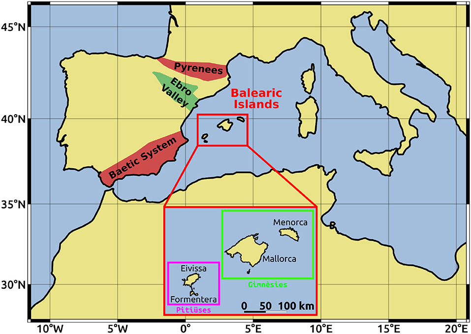
Figure 1. Map of the Western Mediterranean with some geographical features are highlighted. Inset showing the structure of the Balearic Islands. Made with Natural Earth and Open Street Map, © OpenStreetMap contributors.

The archipelago has about 1,700 km of coastline, where 867 beaches make up 10% of that length. The typical Balearic beach appears sparsely along the coast, accommodated in the space allowed by a physiographic control. It is short and narrow; presents features such as rocks, cliffs, and islets; and tends to be at the bottom of a wall-sided embayment. However, 2.4% of the Balearic beaches are longer than 1 km (Gómez-Pujol et al., 2019). According to Gómez-Pujol et al. (2019), who assessed regional shoreline change at the Balearic Islands from 2002 to 2012, 80% of beaches are stable, meaning they do not erode nor accrete more than 50 cm per year.

According to Wright and Short 1984 classification, approximately 20% of the Balearic Islands' beaches are enclosed and present reflective conditions; 42% of them are semi-enclosed, exhibiting intermediate but reflective-skewed conditions; 27% are exposed, non-protected beaches (Gómez-Pujol et al., 2007). The remaining 11% corresponds to anthropic or artificial beaches (generated by the presence of a groin or a dike).

Regarding beach sediment, most beaches are composed of sand, although more than 20% of them are mixed or bigger-sediment beaches. There is no substantial sediment fraction of fluvial origin since water streams in the Balearic Islands are ephemeral. Moreover, the connection to the mainland undergoes depths greater than 800 m, so sediment has a local origin. About 50–75% of sediment is bioclastic, although up to 10–30% of it can be of lithoclastic origin depending on the availability of cliff-detached material (Gómez-Pujol et al., 2007). The leading producer of biogenic material is the endemic seagrass Posidonia oceanica (Fornos and Ahr, 1997). It colonizes nearshore zones all around the Balearic Islands and provides housing to a variety of marine species. It also stabilizes submerged beach sediment and attenuates wave energy (Infantes et al., 2009).

Concerning marine forcings, the Balearic Islands' beaches are microtidal: the spring tidal range is smaller than 25 cm (Orfila et al., 2005). Regional winds are moderate and have a short fetch. As a result, they produce moderately short period waves: the typical significant wave height (H_s) range is 0.1–1 m and the associated periods are between 3 and 6 s (Alvarez-Ellacuria et al., 2011). The mean incoming wave direction is from the north and the north-west, caused by the Pyrenees and the Ebro valley (see Figure 1). The most energetic conditions occur between December and January, and the least ones during June and August (Cañellas et al., 2007). However, frontogenetic activity is very relevant in the basin (i.e., many atmospheric fronts are generated in the region), producing a large variability in wave regime (Morales-Márquez et al., 2020).

Beach morphodynamics is mainly controlled by wave climate: the cross-shore coordinate is controlled by wave height and wave period, while the alongshore also depends on wave energy flux. For the few cases with available data, beach planform is stable (meaning no significant changes occur in the wave energy flux direction) and presents a seasonal cross-shore variation, which consists of an aerial beach loss during severe storms and a gradual recovery during mild wave conditions (Enŕıquez et al., 2017; Morales-Márquez et al., 2018).

Beach tourism has a large impact on the economy of the Balearic Islands, accounting for a 35% of the total Gross Domestic Product (GDP) (Llompart et al., 2020). In 2019 the Balearic Islands received 16.4 million visitors, mostly seeking beach and recreation during summer. This quantity represents more than 10 times the amount of archipelago inhabitants and makes the Balearic Islands one of the most popular destinations in Europe (Llompart et al., 2020).

Regional coastal management has focused on providing leisure services and keeping the backshore functional for recreational uses, with activities such as terrain smoothing, mechanical cleaning, Posidonia oceanica beach wrack (Balestri et al., 2006) withdrawal, and sand nourishments (Roig-Munar et al., 2019).

In the following, we analyze beach erosion and coastal flooding associated with climate change over 192 beaches in Mallorca (ranging 56.9 km of coastline), 132 beaches in Menorca (ranging 21.5 km of coastline), and 140 beaches in the Pitiüuses (ranging 46.1 km of coastline). A complete list of beach names and locations is provided as Supplementary Material, as well as an image showing the distribution of the analyzed beaches (indicated as red dots in “beaches_and_reference_points_and_flooding_zones.png”).

3. Data and Methods

3.1. Regional Mean Sea Level, Storm Surges and Wind-Waves

The marine forcing around the Balearic Islands has been characterized under different scenarios at the regional scale. For flooding analysis, the magnitude of interest is the total water level, defined here as:

$\begin{array}{ll}\text{TWL}=\text{MSL}+\text{WS}+\text{SS}& (1)\end{array}$

where MSL is the mean sea level projected for the different scenarios considered, WS the component associated with the wave setup, and SS the storm surge. The latter two consist of 3-h time series, which add higher-frequency variability. Astronomic tides were omitted in this study. The portion of wave run-up not associated with wave setup was not considered because we focus on coastal extreme water levels that cause temporary flooding at time scales of hours to days. On the contrary, wave run-up acts on shorter time scales around a mean value of sea level.

MSL projections were obtained following Kopp et al. (2014). Figure 2 represents local MSLR projections for RCP4.5 and RCP8.5 climate scenarios. We considered the multi-model ensemble 17 and 83% probabilities, defining a central 67% probability interval (“likely” range in the IPCC report of Stocker et al., 2014).

FIGURE 2

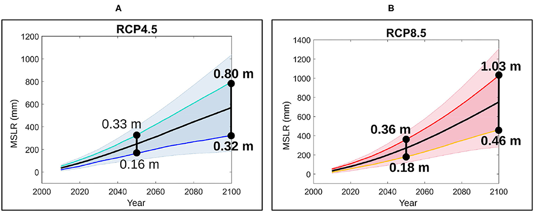
Figure 2. MSLR projections under RCP4.5 (A) and RCP8.5 (B) climate scenarios, calculated according to Kopp et al. (2014). Black lines indicate the multi-model ensemble median and shadowed regions indicate the 17–83% and the 5–95% probability intervals. The four colored lines indicate the MSLR evolutions considered for the analysis of beach erosion, while the six values labeled in bold indicate the MSLR cases considered for the analysis of coastal flooding.

For WS and SS, we used data from Mentaschi et al. (2017) to Vousdoukas et al. (2017), who computed waves with the wind-wave spectral model WaveWatch III (Tolman, 2002), and storm surges with the hydrodynamic model Delft3d-FLOW (Deltares, 2006), consistently forced by atmospheric pressure and surface wind fields from ERA-Interim reanalysis (hindcast spanning the period 1979–2014) and from 6 CMIP5 GCMs for the historical period (1970–1999) and future projections (2070–2099). The temporal sampling of the hindcast is 3 h for H_s and 6 h for SS.

Figure 3 shows the dynamic models' grid points around the Balearic Islands, depicting the differences in the 50-year return period of H_s and SS between the projections and the historical records. Multi-model mean differences for H_s are shown in panels Figure 3A (RCP4.5) and Figure 3C (RCP8.5), while multi-model standard deviations of the differences are shown in panels Figure 3B (RCP4.5) and Figure 3D (RCP8.5). The same information is provided for SS in panels Figures 3E–H. Results indicate that the dispersion of extreme values among the models is larger than the expected changes in most locations. Moreover, it is unlikely to extract a realistic uncertainty from such a limited number of models (the datasets we use for H_s and SS, from Vousdoukas et al. (2017), are obtained from 6 climate models: ACCESS1.0, ACCESS1.3, CSIRO-Mk3.6.0, EC-EARTH, GFDL-ESM2G, GFDL-ESM2M).

FIGURE 3

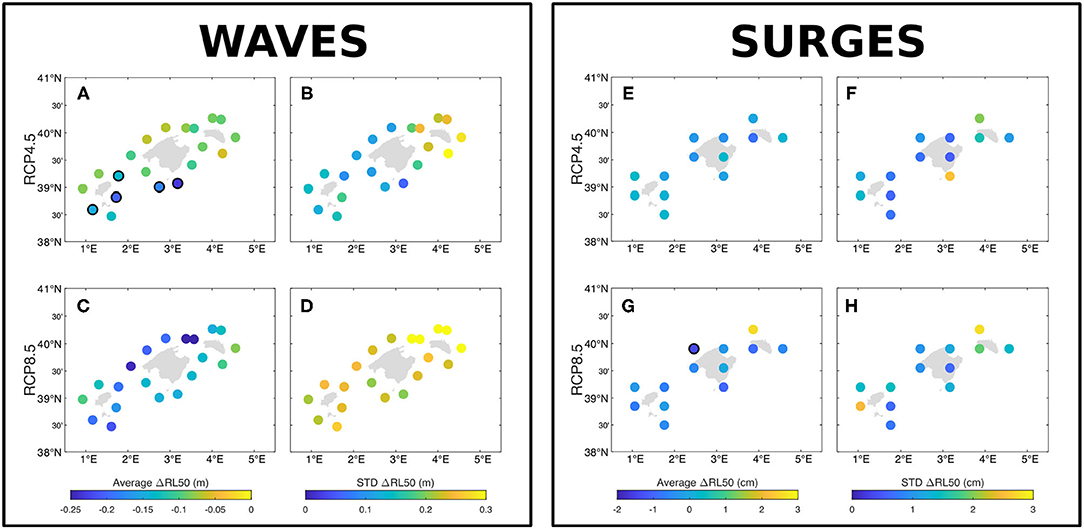
Figure 3. Multi-model mean differences in 50-year return levels between projections (2070–2099) and historical (1970–1999) runs of Hs are shown in panels (A) (RCP4.5) and (C) (RCP8.5), while multi-model standard deviations of the differences are shown in panels (B) (RCP4.5) and (D) (RCP8.5). The same information is provided for SS in panels (E), (F), (G), and (H). Grid points circled black indicate that projected changes are greater than the standard deviation between models.

Consequently, given the unclear tendency and magnitude of the potential change plus the lack of precision in the uncertainty characterization, we decided not to account for any projected change in sea-level extremes. In other words, we assume that wave climate and storm surges will remain unaltered in the future. Therefore, we only used the hindcast outputs for both waves and storm surges, even to compute extremes. This way, we focus on the largest uncertainty (that from mean sea-level projections) and do not consider the others, such as those from storm surges and waves, which is in agreement with a fraction of the existing studies (e.g., Toimil et al., 2017b; Sanuy et al., 2018).

3.2. Wave Propagation

We selected 11 points (virtual buoys) that face all islands' orientations from the wave hindcast described above (see Figure 4). Deepwater conditions of those virtual buoys were propagated up to a set of reference points located about 30 m in depth, considered as representative of nearshore conditions. A map with the reference points locations (indicated as purple stars) is provided as Supplementary Material.

FIGURE 4

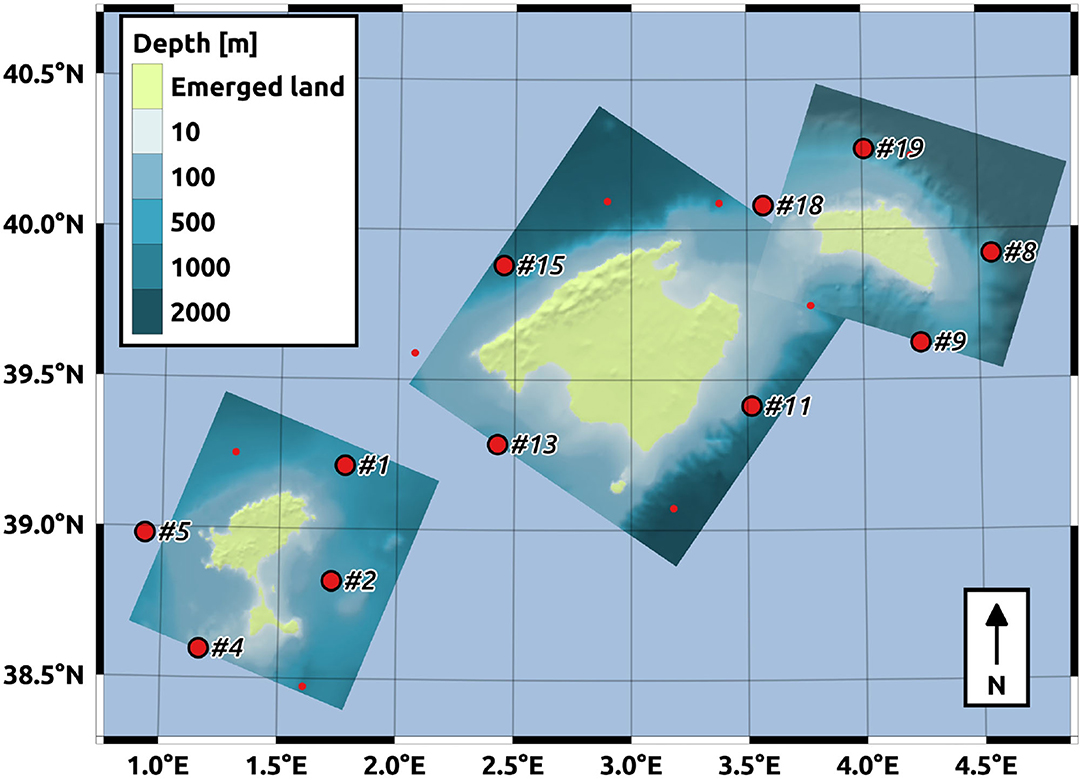
Figure 4. Computational meshes used for wave propagation. Red dots indicate wave hindcast data points (Vousdoukas et al., 2017). Bigger dots indicate the data points we used for propagation (virtual buoys). Meshes are colored according to the bathymetry.

Due to the high computational cost of the 3-h 36-year-long wave hindcast numerical propagation, linear wave theory was applied to build time series of nearshore waves, as described in detail in the following.

Considering a wave propagating over a slowly varying bathymetry, before breaking and in the absence of wind and diffraction, its wave height H_r at depth h_r (before breaking) is related to its deepwater wave height H₀ as Dean and Dalrymple (1991):

$\begin{array}{ll}{\text{H}}_{\text{r}}={\text{H}}_0{\text{K}}_{\text{s}}(\text{T},{\text{h}}_{\text{r}}){\text{K}}_{\text{r}}({\theta }_0)& (2)\end{array}$

where K_s is the shoaling coefficient (which depends on local depth and wave period), and K_r is the refraction coefficient (which depends on the bathymetry and the direction of the wave at deep waters, θ₀). The shoaling coefficient relating the variation in wave height from deep to intermediate waters is given by:

$\begin{array}{ll}{\text{K}}_{\text{s}}=\frac{\text{T}}{2\pi }\sqrt{\frac{\text{g}}{{\text{h}}_{\text{r}}}}\sqrt{\frac{{\text{k}}_{\text{r}}{\text{h}}_{\text{r}}}{1+{\xi }_{\text{r}}}}& (3)\end{array}$

where g is the acceleration of gravity, T is the wave period (which is not modified during propagation), h_r is the water depth at the propagation destination point, k_r is the wave wavelength, and ξ_r = 2k_rh_r/sinh 2k_rh_r. In order to solve Equation (2), it is necessary to infer K_r(θ₀) and, since this equation relates the change in wave height between two specific (though arbitrary) locations, we need to do so for each pair of virtual buoy and reference point. The process to obtain K_r is explained in the following paragraphs. Hereafter, we consider all wave heights as significant wave heights (H_s), all periods as peak periods, and all directions as peak directions.

We classified all hindcast sea states of each deepwater virtual buoy (red dots in Figure 4) in eight octants (waves coming from the N, NE, E, SE, S, SW, W, and NW). Each octant's monthly maximum wave height was propagated (with their corresponding period and direction) over 500 m resolution meshes (shown in Equation 4) using the action balance model SWAN (Booij et al., 1999), by forcing the described sea states along all the mesh side of that virtual buoy and neglecting the effects of wind. Propagations were conducted independently for Mallorca, Menorca, and the Pitiüses, defining a total of 42,528 propagations (3 domains × 4 deepwater points × 8 octants × 443 months). An example of the SWAN configuration file, the code used to generate SWAN forcing files, and the code used to order all SWAN runs are included as Supplementary Material.

For each reference point and deep water virtual buoy, we computed the ratio K_r = H_r/H₀ · 1/K_s relating the wave height at the virtual buoy and the reference point. K_r(θ₀) was estimated by polynomial fitting, using the computed ratios for wave height of all octants at the same time. After a trial and error process, we found a fitting of the form:

$\begin{array}{ll}{\text{K}}_{\text{r}}^{\text{fit}}({\theta }_0)\equiv {\text{p}}_1{\left(1-{\left(abs\left(\frac{{\theta }_0-{\text{p}}_2}{180}\right)\right)}^{{\text{p}}_3}\right)}^{{\text{p}}_4}& (4)\end{array}$

with p₁, p₂, p₃, and p₄ parameters to be adjusted, abs the absolute value and θ₀ (the virtual buoy peak direction) between –180° and +180°. Figure 5 shows an example of fitting, which is representative of the majority of wave propagations. Four time series of wave height for each reference point were obtained applying Equation (2) and the fitted K_r(θ₀). The final 3-h H_s time series, representative of beach wave conditions, was built as the timewise maximum of its four reference points H_s time series. The corresponding T series was defined as the peak period associated with the selected H_s at each time. In line with the regional approach, wave trains were assumed to reach the coast perpendicularly. For this reason, nearshore wave direction time series were not computed. Also, to facilitate the understanding of this explanation, a graphical summary of the wave propagation process is presented as Supplementary Material.

FIGURE 5

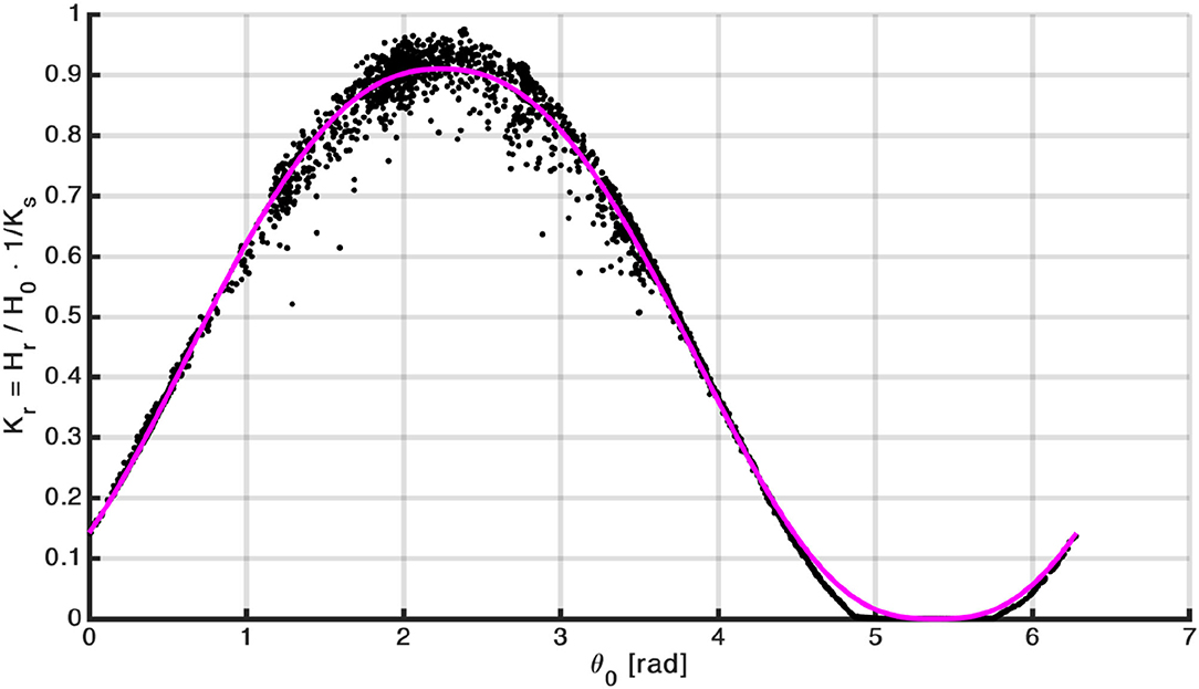
Figure 5. Black dots represent refraction coefficients K_r = H_r/H₀ · 1/K_s computed for one pair of deep water point (virtual buoy) and one reference point vs. virtual buoy peak wave direction (θ₀) for each case. Magenta line indicates the polynomial fitting [Equation (4)] performed over those points.

Many studied beaches receive wave trains from multiple deep-water points (especially those oriented toward the computational domain vertices). However, wave trains that impact an island on one side should not affect the opposite side. We could manually decide which deep-water points should be considered for each beach, but this procedure is subjective and arbitrary. Instead, we assumed that wave trains with any direction coming from any deep-water point could reach (potentially) all beaches and thus we computed all the associated K_r fittings. For the cases where the bulk of and island blocks wave train propagation, the obtained K_r fitting presents small values (near to zero), and the resulting nearshore wave heights associated with those wave trains (computed with Equation 2) are negligible. Since the final nearshore wave height is the maximum among the four propagated waves from deep-water points, our model accounts for shadowing intrinsically.

Regarding diffraction, SWAN does not solve diffraction directly but uses a phase-decoupled approach. This method provides the qualitative behavior of diffraction processes for a restricted set of conditions listed in the technical manual of SWAN (the SWAN team, 2019a). In principle, features large enough to be represented in the 500 m computational meshes induce diffraction in the SWAN model (which can be captured by Equation (2), since K_r is adjusted considering SWAN outputs). However, SWAN needs a grid size five to ten times smaller than the wavelength of a wave train to compute its diffraction adequately (Kim et al., 2017; the SWAN team, 2019b). On the contrary, smaller features are not represented in the computational meshes, and thus their diffraction can not be estimated. Unfortunately, high resolution bathymetries are only available for specific locations. Considering all these reasons, we did not use the diffraction option of SWAN (DIFFRAC). Handling of diffractive obstacles is out of the scope of our regional approximation and is left to future, local studies.

In order to validate the reference points' H_s, we compared our time series with the available in situ data at three coastal locations. The root mean square error at these locations ranges 0.20–0.28 m for H_s and 1.04–1.54 s for T, while the bias (generated time series with respect to measures) takes values between –0.16 and –0.05 m for H_s and between –0.29 and 0.01 s for T. The results and details of the comparison process, as well as the definition of the metrics used, are contained in Appendix A.

3.3. Computation of the Coastal Flooding Extent

Flooding is conducted over multiple zones, selected by considering the beaches under study and the topography, using terrain with high elevation as boundaries. A map with the location of all the flooding zones is provided as Supplementary Material. We employed the topography of “Servei d'Informació Territorial de les Illes Balears” (SITIBSA), as given by its 2 m resolution Digital Surface Model (DSM). The DSM is derived from LiDAR data of 0.5 points/m² point density and whose vertical RMSE is at most 20 cm. It can be consulted at (https://www.caib.es/sites/sitibsa/es/n/mdt-70457/).

3.3.1. Permanent Flooding Induced by MSLR

The values of MSLR used to quantify the permanently flooded coastal areas in 2050 and 2100 were the 17th and 83rd percentiles of both RCP4.5 and RCP8.5 multi-model ensemble spreads (Figure 2).

Permanent flooding was modeled using a bathtub method. Classical bathtub models consider all areas with an elevation below a given MSL as flooded (Yunus et al., 2016; Teng et al., 2017), being computationally cheap and thus suitable for regional assessments. However, they usually neglect physical processes, hence reporting greater flooding extents (Seenath et al., 2016). Aiming to diminish those undesired effects, we performed a multi-step correction over the bathtub results.

The application of our bathtub approach is as follows. First, we use the DSM to create a binary mask under each MSL value, where each DSM pixel is classified as flooded or not flooded depending on whether its elevation is lower or higher than the MSL considered, respectively. This binary map is then manually corrected to ensure surface hydrological connectivity, characterizing those elements misrepresented in the DSM (irrigation channels, thin walls, etc.). Afterward, we identify which binary flooding mask pixels are connected to the sea through a flood-filling algorithm. Flood-filling algorithms take an input point and find all pixels presenting the same value of a certain variable (what is called the region of that pixel), surrounded exclusively by pixels that present a different value on that variable (Rogers, 1998). Here, the initial point is an arbitrary pixel over the open sea, while the region comprises those flooded pixels connected to the initial one by a path made entirely of flooded pixels. After flood-filling, all pixels outside the region are marked as not flooded. Finally, small isolated groups of non-flooded pixels were also classified as flooded since they usually indicate undesired effects over the elevation map. Specifically, we reclassified groups of ≤50 pixels (≤200 m²) if their elevation was lower than 20 cm above the MSL considered, and groups o of ≤100 pixels (≤400 m²) otherwise. For each MSL case, we defined a new coastline as all non-flooded pixels connected with flooded pixels. This coastline was the one considered during the temporary flooding simulations. The whole modified bathtub process is summarized in the Supplementary Material.

3.3.2. Temporary Flooding Induced by Coastal Extreme Sea Levels and MSLR

Coastal extreme sea levels arise from the combination of storm surges (SS) and wave setup (WS), i.e., WS + SS, over the corresponding MSL. The spatial extent of coastal flooding induced by coastal extreme sea levels was simulated, at each flooding zone, with the LISFLOOD-FP model (version 7.0.6, http://www.bristol.ac.uk/geography/research/hydrology/models/lisflood/), which is based on the shallow-water equations (Vreugdenhil, 1994). We performed 1-day simulations over the DSM described above, using the acceleration mode (i.e., neglecting convective acceleration but keeping the local acceleration term in the shallow-water equations), a constant Manning parameter of 0.06, and the default diffusion controlling weighting factor of 0.9 (which modifies the discharge time derivative to incorporate information about the discharge in surrounding cells in such a way that diffusive effects appear, thus reducing numerical instabilities) (de Almeida et al., 2012). An instantaneous sea-level time series was used to force the model along the coastline defined for every MSL value (the ones resulting from our permanent flooding estimation). To apply LISFLOOD-FP over the totality of each flooding zone (this is, including the regions between the beaches of the flooding zone), a single WS + SS time series was forced within each flooding zone, defined as the weighted mean of WS + SS from all the beaches inside this flooding zone, where the weights are the alongshore sizes of each beach. Following Stockdon et al. (2006), the WS of each beach can be estimated as:

$\begin{array}{ll}\text{WS}=0.35{\beta }_{\text{f}}\sqrt{{\text{H}}_0{\text{L}}_0}=0.35{\beta }_{\text{f}}\text{T}\sqrt{\frac{\text{g}}{2\pi }{\text{H}}_0}& (5)\end{array}$

with β_f being the foreshore slope of the beach, and L₀ the peak wavelength at deep waters. The value 0.35 is a constant calibrated using experimental data. We remark that for the second equality of Equation (5) we have assumed deep water conditions. Here, we propose a modification of this equation as:

$\begin{array}{ll}\text{WS}=\alpha {\beta }_{\text{f}}\text{T}\sqrt{\frac{\text{g}}{2\pi }{\text{H}}_{\text{r}}}& (6)\end{array}$

i.e., incorporating reference point's significant wave height (H_r), where α is a factor to be calibrated. H_r is used instead of H₀ to remove those deepwater conditions that do not reach the coast due to their propagation direction. Factor α is obtained by dividing Equation (5) by Equation (6) and using a characteristic value for the ratio H_r/H₀ according to the results of the numerical wave propagation (the value corresponding to the average angle of the H_r/H₀ slopes bigger than 0.05). Foreshore slope β_f is estimated using the distance between the coastline and the –10 m isobath, obtained from the nautical charts of the “Instituto Hidrográfico de la Marina” (this isobath is the shallowest one reported for the set of studied beaches in those nautical charts). We used a different β_f value for each beach, and within each beach we used the same value for all the studied cases (i.e., we assumed that β_f does not change with time or with MSLR).

Extreme values from the weighted WS + SS time series were characterized by fitting a Generalized Pareto Distribution to its exceedances over the 99th percentile. Independence among events was ensured by declustering with a time window of 72 h. The magnitude of the extreme water level event was defined as the fitted Generalized Pareto Distribution 100-year return level and its duration as the median duration of the exceedances (events exceeding the 99th percentile).

Finally, the time series forced over the flooding zone coastline was constructed as a triangular pulse over the corresponding MSL with an intensity and a duration as defined above (we keep sea level at the corresponding MSL after the end of the triangular pulse, until the simulation ends). The decision to use a triangular shape for the forcing is justified in Appendix B. An example of the LISFLOOD configuration for one of the flooding zones is provided as Supplementary Material.

Note that our LISFLOOD setup was not validated in the flooding zones studied due to the lack of measurements. Instead, we performed a sensitivity analysis in one flooding zone (the one presented in of the Supplementary Material). In our case, the only free parameter is the Manning coefficient (since all the other inputs are study design decisions that have been already discussed: mean sea level; extreme event shape, duration, and intensity). The Manning coefficient was varied from 0.006 to 0.6 with a change in the flooding extent lower than 0.04% for MSLR=0; 0.1% for MSLR=18 cm; 5.9% for MSLR=32 cm; 6.9% for MSLR=36 cm; 23.6% for MSLR=46 cm; 4.6% for MSLR=80 cm; and 0.36% for MSLR=103 cm (all of them with respect to the original simulations with Manning coefficient of 0.06). Changes are small except for the case of MSLR=46 cm, coinciding with a big area presenting an elevation near to this value and thus being more sensitive to the Manning coefficient.

3.3.3. Filtering of Water Bodies

Flooding masks were combined with the 2018 Corine Land Cover database, available through Copernicus services (https://land.copernicus.eu/pan-european/corine-land-cover/clc2018). The categories considered were “artificial surfaces” (LU-ART, which include urban areas), “agricultural areas” (LU-AGR), “seminatural areas and forests” (LU-SAF), and “wetlands” (LU-W). We omitted the areas categorized as “water bodies” (LU-WB).

Total flooded areas reported in this manuscript are the sum of the flooding extents categorized as one of the four land-uses we considered. Inner water bodies are not well characterized in the DSM because they are not identified as such. Moreover, interpolation errors occur over them. By removing the areas marked as LU-WB in the Corine database those effects are reduced, since those areas currently flooded (permanently or periodically) are not included in the results.

3.4. Computation of Beach Erosion

Balearic Islands beach sediment has a biogenic origin, without river income. Thus, all the sediment involved in beach erosion and accretion is already within the system. Under these conditions, morphodynamic variability can be split in the cross-shore and alongshore directions. Beaches accommodate maximizing wave energy dissipation, rotating until its alongshore direction is normal to the mean wave energy flux at the breaking point. Cross-shore variability (i. e., beach profiles) is the response to waves (shorter time scales) and to MSL (longer time scales).

That being said, the most accurate way to evaluate a specific beach is to perform a whole 3D simulation taking into account all changes inherent to the different scenarios. However, that is not affordable, neither for a specific beach (up to the 2100 horizon) nor for the regional approach we adopted. Therefore, we were forced to assume some simplifications to the problem.

In the first place, as stated in section 2, only 27% of the Balearic Islands' beaches are open (and thus can freely exchange sediment with its surroundings). Accordingly, we neglected the alongshore transport between the beach and its surroundings. In the second place, generalized information about wave energy flux does not exist, so beach planform changes can not be assessed; moreover, beach planform is stable for the few cases where this information is available. Therefore, alongshore averaged cross-shore beach width was used. In the third place, the number of recreational activities occurring at beaches depends directly on the aerial beach surface, equivalent through the alongshore beach size to the average cross-shore beach width. Since we focused on an alongshore-averaged magnitude, internal alongshore transport (i.e., occurring between the beach and itself).

Because of these reasons, we quantified beach erosion as the average cross-shore beach width recession. Classically, the Bruun Rule (Bruun, 1962) has been used for this purpose. It indicates that the beach tends to an equilibrium state whose changes in shoreline can be described (in the form presented by Dean, 1991) as:

$\begin{array}{ll}\Delta \text{y}=-{\text{W}}_{*}·\frac{\text{S}}{\text{B}+{\text{h}}_{*}}& (7)\end{array}$

where Δy is the (seawards) change in equilibrium beach shoreline position with respect to a reference sea level, S indicates the elevation of sea level with respect to that reference, B is the berm height, h_* is the breaking depth, and W^* is the active profile width, computed as ${\text{W}}^{*}={({\text{h}}_{*}/\text{A})}^{3/2}$ (Dean, 1991), where $\text{A}=0.067{\omega }_s^{0.44}$, with ω_s being the settling velocity of mean sand diameter (D50) (van Rijn, 1984). According to similarity theory, the following relation holds at the breaking point: H_b/h_* = κ, where H_b the wave height over breaking depth, and κ is the breaker index (which we assumed to be 0.71).

As stated in section 2, most of the Balearic Islands' beaches lack accommodation space, either because of heavy urbanization or because of natural physiographic controls (pocket beaches in front of cliff walls). In line with our regional approximation, we assumed the backshore of all beaches would remain fixed, so shoreline position changes equal to cross-shore beach width changes (Δy = Δw). Taking this into consideration, using the current mean sea level (MSL₀) as the sea-level reference, and neglecting changes in sea level other than MSLR, Equation (7) can be rewritten as:

$\begin{array}{ll}\Delta \text{w}=\text{w}-{\text{w}}_0=-{\left(\frac{{\text{H}}_{\text{b}}}{\kappa \text{A}}\right)}^{3/2}·\frac{\text{MSL}-{\text{MSL}}_0}{\text{B}+{\text{H}}_{\text{b}}/\kappa }& (8)\end{array}$

w₀ is the equilibrium beach width for the case MSL = MSL₀ and w the equilibium beach width for a MSLR equal to MSL − MSL₀.

Bruun's Rule has some limitations since it assumes a constant wave climate, a constant sediment budget, and the existence of a depth of closure, and also neglects the effect of longshore sediment transport gradients. However, given the nature, dynamics and physiography of the analyzed beaches, as well as the regional context of the study, Bruun's Rule provides an acceptable first approach to the expected beach width changes.

Regarding to the rest of variables needed, according to Gómez-Pujol et al. (2019) beaches in the Balearic Islands are in equilibrium, and so we assumed w₀ as the one measured by the most recent orthographic aerial photographs. For each beach, we estimated a single B value considering the LiDAR point cloud used to generate SITIBSA's DSM. Wave height was computed at different depths by propagating the wave height time series of the beach reference point (H_r), first to deep waters and then to the desired depth. We accomplished that using Equation (2) and assuming K_r equal to one.

Following Toimil et al. (2017a), we applied Equation (8) to a set of multiple synthetic time series of H_b, thus producing multiple potential realizations of beach width evolution. Our synthetic H_b time series are statistically consistent with the corresponding reference point time series at every site (i. e., they have the same statistics but with a different chronology). Since the set of synthetic time series generated is representative of the potential future conditions, the resulting realizations of beach width time series can be used to estimate the statistics of the future beach width evolution. The details of the synthetic time series generation process and its validation are described in Appendix C.

For each beach, we generated 500 synthetic H_b time series and inputted them into Equation (8), in combination with the projected evolutions of MSLR corresponding to the 17 and 83% of RCP4.5 and RCP8.5, obtaining 500 time series of w for each MSLR evolution, from which mean beach width evolution and standard deviation were computed. Since both metrics presented a strong seasonality, resulting time series were filtered with a 5-year running average.

3.5. Beach Recreational Services Monetary Valuation

Beach narrowing due to erosion resulting from our analyzes was used to estimate the decrease or loss of beach recreational services in monetary terms. We adopted the results presented in Enríquez and Bujosa Bestard (2020), who measured the economic impact of beach loss on beach tourism through choice experiments focused on the Balearic Islands. Other works also assessed the recreational services provided by beaches at the Balearic Islands (Pérez-López and Roig-Munar, 2007; Riera et al., 2007), but their surveys were not focused on climate change impacts or on the tourists that comprise the largest portion of yearly beach users in the entire archipelago. Enríquez and Bujosa Bestard (2020) specifically assessed tourists' willingness to pay for the introduction of policies aimed at reducing climate change impacts.

Choice experiment methodology is a stated preference non-market valuation methodology based on experimental surveys. In these surveys respondents are presented with different scenarios describing specific changes in the levels of the good under valuation (in this case the surface of aerial beach) and are asked to choose the scenario providing the highest level of well-being. This is a standard method to assess economic impacts of climate change (Shoyama et al., 2013; Andreopoulos et al., 2015; Remoundou et al., 2015; Rodrigues et al., 2016; Chaikaew et al., 2017; Torres et al., 2017; Faccioli et al., 2019).

In their assessment, they estimated that tourists are willing to pay 1.23 €/day of stay (on average) to recover one meter of beach shoreline to compensate beach retreat due to MSLR. Using this value we estimated the loss of beach recreational value in monetary terms. In this regard, we combined the data obtained in section 3.4 with the Enríquez and Bujosa Bestard (2020) results, as well as with different attributes of each beach (beach location, type, accessibility, etc.) to determine the beach recreational economic value loss (BREV) as follows:

$\begin{array}{l}{\text{BREV}}_{\text{n}}\left(\frac{\text{€}}{\text{yr}}\right)=\frac{{\text{WEBS}}_{\text{n}}({\text{m}}^2)}{{\displaystyle {\sum }_{\text{n}}}{\text{WEBS}}_{\text{n}}\left({\text{m}}^2\right)}·{\text{TOUR}}_{\text{n}}(\text{tourists})\\ ·\text{WTPV}\left(\frac{\text{€}}{\text{m }·\text{ yr}}\right)·{\text{ER}}_{\text{n}}(\text{m})& (9)\end{array}$

where BREV_n is the loss of beach recreational economic value for a specific beach, WEBS_n is the weighted effective beach surface for a specific beach, TOUR_n is the number of tourists (corresponding to the 2019 official estimate of the Balearic Islands Institute of Statistics, IBESTAT), WTPV is the amount of money each tourist is willing to pay in constant monetary units for an individual day of stay considering the average stay length of 6 days (Llompart et al., 2020), and ER_n is the averaged shoreline retreat for each beach obtained in section 3.4.

Beaches in the Balearic Islands tend to be high-frequented (Mas Parera and Blázquez-Salom, 2005; Roig-Munar et al., 2020). In a small island (as each one of the Balearics, with travel times from one side to another lower than 1 h) tourists move from one beach to another. For this reason, the number of users is mainly related to the available dry beach surface. The articles cited above also indicate that the most frequented beaches are those that are in front of tourist stations and also those iconic virgin beaches publicized in touristic guides and brochures. Therefore, according to this descriptive data, we obtain the weighted effective beach surface for a specific beach by means of:

$\begin{array}{ll}{\text{WEBS}}_{\text{n}}({\text{m}}^2)={\text{S}}_{\text{n}}({\text{m}}^2)·{\text{F}}_{\text{type}}·{\text{F}}_{\text{access}}& (10)\end{array}$

where S_n is the beach surface for a specific beach; F_type is a correction factor that introduces the typology of beach that, ranging from 0.5 for isolated beaches to 1 for urban beaches and isolated iconic beaches (Table 1), as the two latter ones comprise most of the demand (Roig-Munar et al., 2020); F_access is a correction factor related with the beach accessibility (access, public transport, parking facilities) and beach recreation services (beach cleaning, sun huts, lifeguards.), creating a variation from 0.05 to 1 according to Table 1.

TABLE 1

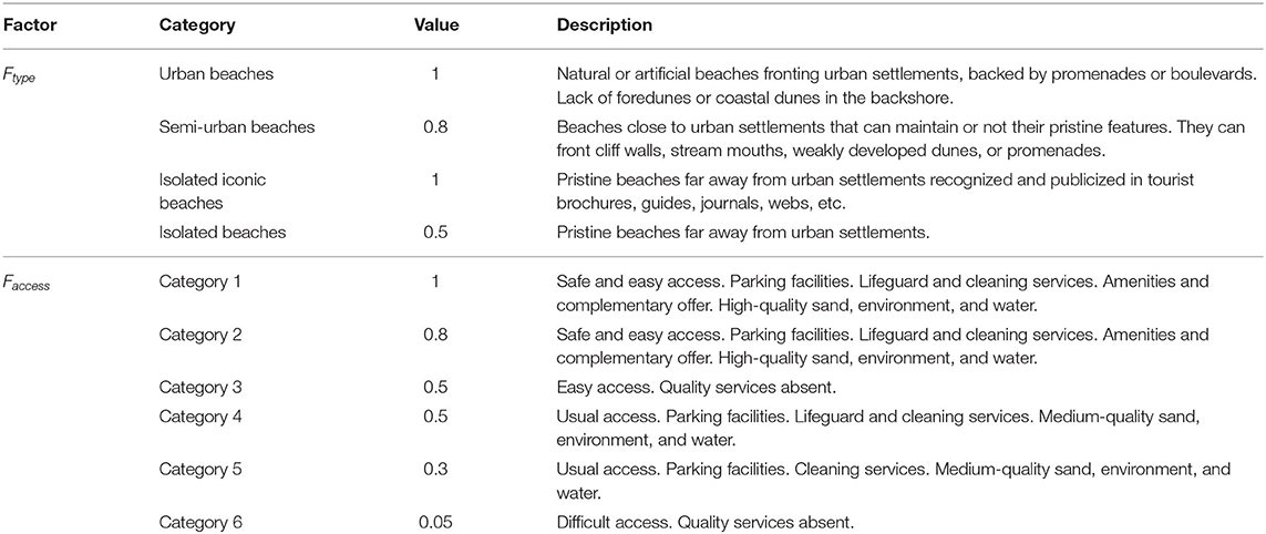
Table 1. Location-based beach correction factor typologies and correction factors derived from beach accessibility and quality services.

4. Results for Coastal Flooding

The results of areas permanently and temporarily flooded due to MSLR combined with storm surges and extreme waves are summarized in Table 2, separately for each region, and classified by its land use. Note that temporary flooding due to extreme events is indicated as increases with respect to permanent flooding induced by MSLR only. Total extent of flooding in the case of extreme events is the addition of the two. Also, note that results are listed in terms of increases in MSL rather than in time horizons. All values reported in the table correspond to either mid or late twenty-first century (see Figure 2 for the equivalence between timing and value of MSLR). The complete set of flooding extent masks can be consulted online at https://ideib.caib.es/impactes_costa_canvi_climatic/. Finally, note that those are estimates for the case that no action is taken. Figure 6 shows the permanent flooding extent for a MSLR of 103 cm over the entire archipelago, classified by municipalities.

TABLE 2

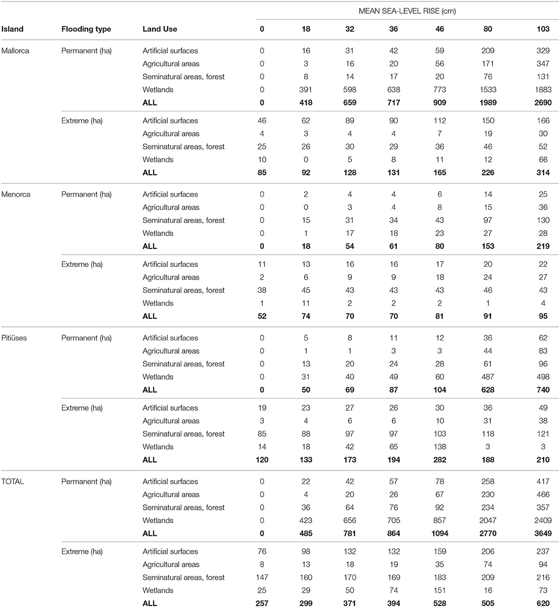
Table 2. Coastal flooding extent (in hectares) resulting from the permanent and temporary flooding analysis.

FIGURE 6

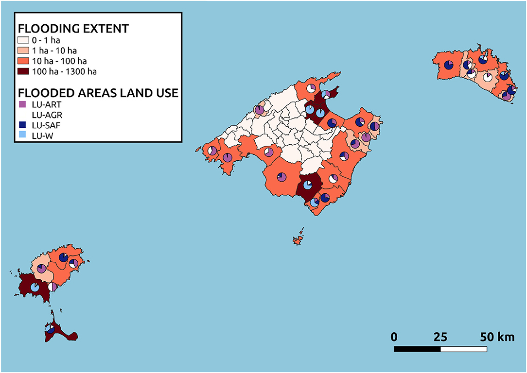
Figure 6. Permanent flooding extent (classified by municipality) for the case of 103 cm of MSLR, with information on land use of flooded areas. Each municipality polygon is colored according to its flooding extent, and has a circular symbol containing the fractions of land use composing that extent (LU-ART, LU-AGR, LU-SAF, LU-W; see Section 3.3.3 for the land use classification).

The area permanently flooded increases linearly with MSLR. Namely, in Mallorca flooding extent changes 24 ha/cm of MSLR (R² of 0.977), in Menorca 2 ha/cm of MSLR (R² of 0.975) and at the Pitiüses the rate reaches 33 ha/cm of MSLR (R² of 0.956). Due to the different coastal lengths, absolute values of flooded extents are clearly dissimilar, ranging between areas up to thousands of hectares in Mallorca to a few hundreds of hectares in Menorca and Pitiüses, for MSLR above 0.5 m. Temporary flooding caused by coastal extreme sea levels increases mostly in Mallorca and Pitiüses (100–300 ha) and is smaller in Menorca, due to the more elevated coastal land.

In terms of relative impacts of flooding, by mid-century and under RCP8.5 (MSL between 18 and 36 cm), permanent flooding reaches between 4.9 and 8.6 km² (0.10–0.17% of the archipelago surface), while extreme flooding adds an extra loss of 0.06 –0.07% to the archipelago land surface. This represents an increase of 16–53% with respect to the flooding extent of an extreme event occurring today. We expect these quantities to be very similar to those of RCP4.5 for the same time horizon.

Likewise, by the end of the century, under the RCP4.5 scenario (MSLR between 32 cm and 80 cm), the permanent flooding extent would fall between 7.8 and 27.7 km² (0.16–0.56% of the archipelago surface). Extreme flooding represents an extra 0.07–0.10% of archipelago surface, which is 44–96% bigger than the extreme flooding extent of the present. Under RCP8.5 scenario (46 cm and 103 cm limits) permanent flooding can extend up to 10.9–36.5 km² (0.20–0.70% of the archipelago surface) and extreme flooding adds 0.11–0.12%, an increase of 105–141% with respect to the extreme flooding that may occur nowadays.

5. Results for Beach Erosion

A compilation of the results for all the beaches is represented in Figure 7 as the CDF of the relative widths with respect to their present state for mid and late twenty-first century. Note that those are estimates for the case that no action is taken.

FIGURE 7

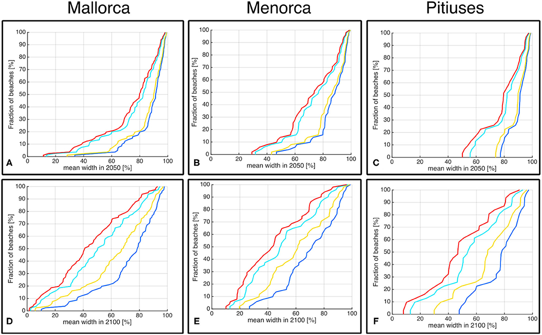
Figure 7. Cumulative density functions (CDF) of beach relative mean width (referred to nowadays width), computed from the time averaged mean evolutions of each beach according to the MSL forcing of the RCP4.5 and RCP8.5 scenarios (lower and upper bounds). Each panel line corresponds to a MSL evolution, using the color code presented in Figure 2. (A–C) Use data extracted from year 2050, and (D–F) Use data from 2100. CDFs are computed for beaches of Mallorca (A,D), Menorca (B,E) and the Pitiüses (C,F).

Around 2050, beach width distributions obtained for the lower and upper limits of RCP4.5 and RCP8.5 are similar. In Mallorca and Menorca around 3–15% of beaches are projected to lose half of their current surface, 0% in the Pitiüses. Between 25 and 55% of the beaches are projected to reduce their present area by less than 10%. Changes are significantly larger by the end of the century. Under the RCP4.5 scenario up to 10% of the Balearic Islands' beaches will lose 90% of the current area. 20–50% of the beaches in Mallorca, 15–50% in Menorca and 5–40% in the Pitiüses are projected to reduce their current size by half. In the worst-case scenario, under RCP8.5 by 2100, up to 15% of the archipelago beaches are expected to lose more than 90% of their surface, while 25–60% of beaches in Mallorca, 35–65% of beaches in Menorca and 23 –60% of beaches in the Pitiüses will lose more than 50% of their current surface. In order to illustrate the spatial distribution of beach erosion, Figure 8 shows the beach surface loss between the present and the 2100 RCP8.5 upper limit of MSLR projection classified by municipality.

FIGURE 8

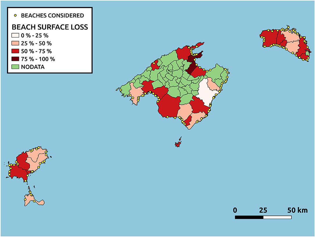
Figure 8. Aerial beach surface loss by 2100 under the RCP8.5 upper limit of MSLR, relative to that of today, classified by municipality. Beaches considered are also shown.

6. Coastal Flooding Impacts on Land Use

The classification of the extent of flooded areas by their land use, according to Corine 2018, is listed in Table 2. Note that those are estimates for the case that no action is taken. Our analyzes demonstrate that wetlands are disproportionally affected by coastal flooding in the Balearic Islands, being clearly dominant in Mallorca and Pitiüses. Overall, these areas represent 65–85% of the total permanently flooded surface. In Menorca, semi-natural areas and forests are the most impacted. Flooding of coastal wetlands increases fast as MSL rises up to 0.5 m, due to their typical low elevation gradient. Above this value these impacts stabilize, indicating that the totality of coastal wetlands is lost. It must be mentioned that we have neglected the dynamic response of coastal wetlands, which may accrete in response to mean sea-level changes, depending on the rising rate and the space availability for sediment accumulation (Schuerch et al., 2018). The latter is rather limited in our case studies, though, but still our estimates should be considered as an upper bound for the given MSLR values.

The areas most affected by coastal flooding, coinciding with the low-lying regions, are formed essentially by lagoons and salt evaporation ponds. There are five flooding zones that account for 85% of the extent of total permanent flooding in the worst-case scenario (MSLR of 103 cm). These are concentrated in the North of Mallorca Island (Alcúdia, Pollença), the South of Mallorca (es Trenc), and parts of Eivissa and Formentera. Therefore, coastal flooding impacts are unevenly distributed around the archipelago. These results are relevant for public policies regarding the prioritization of most vulnerable coastal areas to MSLR.

Frequently, large areas are projected to be flooded because of the presence of a narrow connection to the sea, such as channels, torrents, or salt work entrances. This is illustrated in Figures 9A,B, where Port of Alcúdia flooding zone is the most paradigmatic example: the vast majority of its streets and multiple channels allow flooding of the urban nucleus and the wetland area due to MSLR. The city of Eivissa (Figures 9C,D) includes a good example of an artificially guided torrent.

FIGURE 9

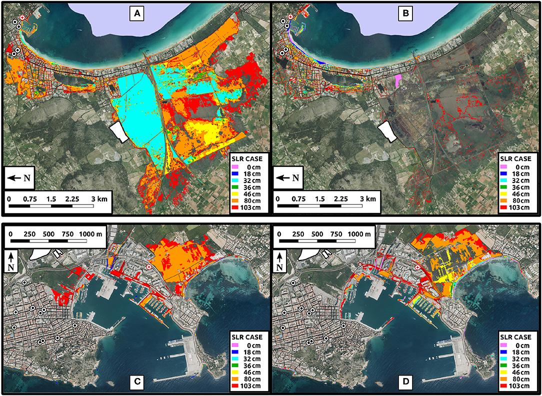
Figure 9. Permanent and extreme flooding extent over the Alcúdia wetland (A,B) and city of Eivissa (C,D). Roads and streets are marked using black lines. Education facilities are indicated as black dots, sanitary buildings as red crosses, and energy production plants as white polygons.

In these maps, public facilities such as schools, sanitary buildings as well as energy infrastructure are marked to illustrate the utility of the assessment to identify critical infrastructures at risk. Major impacts on infrastructures and equipment affect streets, secondary roads, and tracking pathways. This is quite evident in Figures 9A,B, where urban streets at tourist stations and rural secondary roads communications become flooded, especially for MSLR larger than 40 cm. Municipalities are the administration in charge of the most affected communication and transport infrastructure. The power plant at the Alcúdia Bay (Figure 9A) or the Eivissa airport are not affected by MSLR, neither by the associated extreme events, but they will be resting closer to the shoreline. Permanent and eventual floods do not affect any sanitary equipment (Figure 9), while some educational equipment may be damaged at Alcúdia bay (1 school and 1 institute, Figures 9A,B) and Eivissa (1 school, Figures 9C,D) if MSLR surpasses 46 cm.

Figure 6 shows the fraction of permanent flooding extent associated to each land use considered, by municipalities, for the case of 103 cm of MSLR, for the entire archipelago.

7. Loss of Recreational Value Due to Beach Erosion

The estimated losses of recreational value in the beaches of the Balearic Islands are shown in Table 3 for each island separately and for the entire archipelago. Note that those are estimates for the case that no action is taken. The loss ranges from 415 to 827 million euros under RCP4.5 for 2050, from 481 to 932 million euros under RCP8.5 for 2050, from 1,000 to 2,067 million euros under RCP4.5 for 2100, and from 1,421 to 2,428 million euros under RCP8.5 for 2100.

TABLE 3

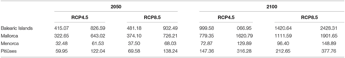
Table 3. Loss of beach recreational services in monetary value (millions of euros) under RCP4.5 and RCP8.5 climate change scenarios for 2050 and 2100.

Under the RCP8.5 scenario, beach recreational services loss by 2050 could represent between 1.4 and 2.8% of the 2019 Balearic Islands GDP, while by 2100 it represents between 4 and 7% of the 2019 Balearic Islands GDP. The Balearic Islands GDP is estimated at 33,800 million euros for 2019.

It should be noticed that this economic value refers to services provided for tourism recreation, not including the local population. Otherwise, beaches provide other additional environmental services, such as coastal protection. In monetary terms, the most damaged beaches of the archipelago under the RCP8.5 scenario in 2100 correspond with the largest beaches located in the major coastal basins of the island: Alcúdia beach in the northern coast of Mallorca and “s'Arenal” in the southern coast of Mallorca, with 574 and 169 million euros of recreational services loss, respectively. In Eivissa, “Platja d'en Bossa” is the most affected beach, with a loss of recreational services equivalent to 147 million euros, whereas the rest of the beaches of the island remain one order of magnitude below this value. The impact on Menorca beaches, in terms of recreational economic value, is lower than in the rest of the islands. The largest impact belongs to Son Bou beach (southern Menorca) with a recreational service loss equivalent to 38 million euros for 2100 under the RCP8.5 scenario.

8. Concluding Remarks

In this work, we estimated the extent of coastal flooding and beach erosion along sandy coastlines in the Balearic Islands as a result of projected MSLR during the twenty-first century. These coastal impacts were quantified for two climate change scenarios, namely RCP4.5 and RCP8.5, combining regional projected MSLR and marine extreme events caused by waves and storm surges. Our analysis constitutes the first study of mean sea-level rise impacts in the Balearic Islands at the regional scale, comprising all sandy coasts. Due to the size of the study site, the analysis was conducted as a regional approach, meaning that we considered a series of methodological approximations. Most of these approximations are related to beach erosion. We assumed that shoreline retreat was equivalent to beach width loss, while those beaches without an urbanized backshore will just displace landwards, as stated by Cooper et al. (2020). Also, we used Bruun's Rule for the computation of beach shoreline evolution which, although provides an acceptable first approach to the expected beach width changes, possess many limitations. For this reason, we believe future studies using more advanced models, such as that of McCarroll et al. (2021), should be conducted.

The approach permitted to identify the potentially most affected areas in the region: the wetlands of Alcúdia, Pollença and es Trenc in Mallorca, and the saltworks of Eivissa (accounting for 85% of the 103 cm of MSLR permanent flooding); as well as the number of beaches undergoing a critical state of erosion: up to 60% of beaches in the region may erode more than a 50% of its current width for a MSLR of 103 cm. Thus, our results can be used to inform the regional and national administrators about the most critical zones in order to prioritize their actuation.

The estimated loss of recreational value for the considered beaches is estimated between 1.4 and 2.8% of 2019 Balearic Islands GDP by 2050 and between 4.2 and 7.2% by 2100, under the worst-case scenario. Importantly, these values do not include the value provided by other beach services such as its role in coastal protection.

Data Availability Statement

The raw data supporting the conclusions of this article will be made available by the authors, without undue reservation.

Author Contributions

LG-P, MM, and AO conceived the idea of the study with the support of PL. PL, LG-P, MM, and AO developed the methodology. PL produced the results with the support of LG-P, MM, and AO. All authors analyzed the results and equally contributed to writing the manuscript.

Funding

This study was supported by PIMA ADAPTA-Balears Project funded by Conselleria de Transició Energética, Sectors Productius i Memòria Democràtica, Govern Balear, and by the FEDER/Ministerio de Ciencia, Innovación y Universidades - Agencia Estatal de Investigación through the MOCCA project (RTI2018-093941-B-C31 MINECO-AEI-UE-FEDER). LG-P is also funded by the CGL2016-79246-P MINECO-AEI-UE-FEDER project. PL was supported by the FPU19/03081 grant from Ministerio de Ciencia, Innovación y Universidades of Spain.

Conflict of Interest

The authors declare that the research was conducted in the absence of any commercial or financial relationships that could be construed as a potential conflict of interest.

The reviewer DI declared a past co-authorship with one of the authors, MM, to the handling editor.

Publisher's Note

All claims expressed in this article are solely those of the authors and do not necessarily represent those of their affiliated organizations, or those of the publisher, the editors and the reviewers. Any product that may be evaluated in this article, or claim that may be made by its manufacturer, is not guaranteed or endorsed by the publisher.

Acknowledgments

We want to thank the Balearic Islands Coastal Observing and Forecasting System (SOCIB), who shared their data and collaborated collectively during the development of this project. We are grateful to Jeffrey Neal from the University of Bristol for sharing the latest version of LISFLOOD-FP. Comments from our three referees are greatly appreciated.

Supplementary Material

The Supplementary Material for this article can be found online at: https://www.frontiersin.org/articles/10.3389/fmars.2021.676452/full#supplementary-material

References

Alvarez-Ellacuria, A., Orfila, A., Gómez-Pujol, L., Simarro, G., and Obregon, N. (2011). Decoupling spatial and temporal patterns in short-term beach shoreline response to wave climate. Geomorphology 128, 199–208. doi: 10.1016/j.geomorph.2011.01.008

CrossRef Full Text | Google Scholar

Andreopoulos, D., Damigos, D., Comiti, F., and Fischer, C. (2015). Estimating the non-market benefits of climate change adaptation of river ecosystem services: a choice experiment application in the aoos basin, greece. Environ. Sci. Policy 45, 92–103. doi: 10.1016/j.envsci.2014.10.003

CrossRef Full Text | Google Scholar

Balestri, E., Vallerini, F., and Lardicci, C. (2006). A qualitative and quantitative assessment of the reproductive litter from posidonia oceanica accumulated on a sand beach following a storm. Estuarine Coastal Shelf Sci. 66, 30–34. doi: 10.1016/j.ecss.2005.07.017

CrossRef Full Text | Google Scholar

Booij, N., Ris, R. C., and Holthuijsen, L. H. (1999). A third-generation wave model for coastal regions: 1. Model description and validation. J. Geophys. Res. 104, 7649–7666. doi: 10.1029/98JC02622

CrossRef Full Text | Google Scholar

Bruun, P. (1962). Sea-level rise as a cause of shore erosion. J. Waterways Harbors Div. 88, 117–130. doi: 10.1061/JWHEAU.0000252

CrossRef Full Text | Google Scholar

Cañnellas, B., Orfila, A., Méndez, F. J., Menéndez, M., Gómez-Pujol, L., and Tintoré, J. (2007). Application of a POT model to estimate the extreme significant wave height levels around the Balearic Sea (Western Mediterranean). J. Coastal Res. 50, 329–333.

Google Scholar

Chaikaew, P., Hodges, A. W., and Grunwald, S. (2017). Estimating the value of ecosystem services in a mixed-use watershed: a choice experiment approach. Ecosyst. Serv. 23, 228–237. doi: 10.1016/j.ecoser.2016.12.015

CrossRef Full Text | Google Scholar

Cooper, J. A. G., Masselink, G., Coco, G., Short, A. D., Castelle, B., Rogers, K., et al. (2020). Sandy beaches can survive sea-level rise. Nat. Clim. Chang 10, 993–995. doi: 10.1038/s41558-020-00934-2

CrossRef Full Text | Google Scholar

de Almeida, G. A. M., Bates, P., Freer, J. E., and Souvignet, M. (2012). Improving the stability of a simple formulation of the shallow water equations for 2-D flood modeling. Water Resour Res. 48:W05528. doi: 10.1029/2011WR011570

CrossRef Full Text | Google Scholar

Dean, R. G. (1991). Equilibrium beach profiles: characteristics and applications. J. Coastal Res. 7, 53–84.

Google Scholar

Dean, R. G., and Dalrymple, R. A. (1991). Water Wave Mechanics for Engineers and Scientists, Vol. 2 of Advanced Series on Ocean Engineering. World Scientific.

Google Scholar

Deltares (2006). Simulation of Multi-Dimensional Hydrodynamic Flows and Transport Phenomena, Including Sediments. Delft: Deltares.

Google Scholar

Enríquez, A. R., and Bujosa Bestard, A. (2020). Measuring the economic impact of climate-induced environmental changes on sun-and-beach tourism. Clim Change 160, 203–217. doi: 10.1007/s10584-020-02682-w

CrossRef Full Text | Google Scholar

Enríquez, A. R., Marcos, M., Álvarez-Ellacuría, A., Orfila, A., and Gomis, D. (2017). Changes in beach shoreline due to sea level rise and waves under climate change scenarios: application to the Balearic Islands (Western Mediterranean). Natural Hazards Earth Syst. Sci. 17, 1075–1089. doi: 10.5194/nhess-17-1075-2017

CrossRef Full Text | Google Scholar

Faccioli, M., Kuhfuss, L., and Czajkowski, M. (2019). Stated preferences for conservation policies under uncertainty: insights on the effect of individuals' risk attitudes in the environmental domain. Environ. Resour. Econ. 73, 627–659. doi: 10.1007/s10640-018-0276-2

CrossRef Full Text | Google Scholar

Fornos, J. J., and Ahr, W. M. (1997). Temperate carbonates on a modern, low-energy, isolated ramp: the Balearic Platform, Spain. SEPM J. Sediment. Res. Vol. 67. doi: 10.1306/D4268572-2B26-11D7-8648000102C1865D

CrossRef Full Text | Google Scholar

Gómez-Pujol, L., Orfila, A., Ca nellas, B., Alvarez-Ellacuria, A., Méndez, F. J., Medina, R., et al. (2007). Morphodynamic classification of sandy beaches in low energetic marine environment. Mar. Geol. 242, 235–246. doi: 10.1016/j.margeo.2007.03.008

CrossRef Full Text | Google Scholar

Gómez-Pujol, L., Orfila, A., Morales-Márquez, V., Compa, M., Pereda, L., Fornós, J. J., et al. (2019). “Beach systems of Balearic Islands: nature, distribution and processes,” in The Spanish Coastal Systems: Dynamic Processes, Sediments and Management, ed J. A. Morales (Cham: Springer International Publishing), 269–287.

Google Scholar

Infantes, E., Terrados, J., Orfila, A., Canellas, B., and Alvarez-Ellacuria, A. (2009). Wave energy and the upper depth limit distribution of Posidonia oceanica. Bot. Mar. 52, 419–427. doi: 10.1515/BOT.2009.050

CrossRef Full Text | Google Scholar

Jiménez, J., Osorio, A., Marino-Tapia, I., Davidson, M., Medina, R., Kroon, A., et al. (2007). Beach recreation planning using video-derived coastal state indicators. Coastal Eng. 54, 507–521. doi: 10.1016/j.coastaleng.2007.01.012

CrossRef Full Text | Google Scholar

Kay, S. M. (1993). Fundamentals of Statistical Signal Processing. Prentice Hall Signal Processing Series. Prentice-Hall PTR.

Google Scholar

Kim, G. H., Jho, M. H., and Yoon, S. B. (2017). Improving the performance of swan modelling to simulate diffraction of waves behind structures. J. Coastal Res. 79, 349–353. doi: 10.2112/SI79-071.1

CrossRef Full Text | Google Scholar

Kopp, R. E., Horton, R. M., Little, C. M., Mitrovica, J. X., Oppenheimer, M., Rasmussen, D. J., et al. (2014). Probabilistic 21st and 22nd century sea level projections at a global network of tide-gauge sites. Earths Future 2, 383–406. doi: 10.1002/2014EF000239

CrossRef Full Text | Google Scholar

Lionello, P., Abrantes, F., Congedi, L., Dulac, F., Gacic, M., Gomis, D., et al. (2012). Introduction: Mediterranean Climate—Background Information. Oxford: Elsevier, XXXV–XC.

Google Scholar

Llompart, M., Sergio, B., Díaz, J. G., Lora, S., Montejano, S., and Navinés, F. (2020). Memòria del Consell Econòmic i Social de les Illes Balears sobre l'economia, el treball i la societat de les Illes Balears 2019. Technical Report 2019, Consell Econòmic i Social de les Illes Balears, Palma, Spain.

Google Scholar

Mas Parera, L., and Blázquez-Salom, M. (2005). Anàlisi de la freqüentaciò d'ús a les platges i estudi de paràmetres de sostenibilitat associats. Doc. Anàl. Geogr. 45, 15–40.

Google Scholar

McCarroll, R. J., Masselink, G., Valiente, N. G., Scott, T., Wiggins, M., Kirby, J.-A., et al. (2021). A rules-based shoreface translation and sediment budgeting tool for estimating coastal change: shoretrans. Ma.r Geol. 435:106466. doi: 10.1016/j.margeo.2021.106466

CrossRef Full Text | Google Scholar

Mentaschi, L., Vousdoukas, M. I., Voukouvalas, E., Dosio, A., and Feyen, L. (2017). Global changes of extreme coastal wave energy fluxes triggered by intensified teleconnection patterns. Geophys. Res. Lett. 44, 2416–2426. doi: 10.1002/2016GL072488

CrossRef Full Text | Google Scholar

Morales-Márquez, V., Orfila, A., Simarro, G., Gómez-Pujol, L., Álvarez-Ellacuría, A., Conti, D., et al. (2018). Numerical and remote techniques for operational beach management under storm group forcing. Natural Hazards Earth Syst. Sci. 18, 3211–3223. doi: 10.5194/nhess-18-3211-2018

CrossRef Full Text | Google Scholar

Morales-Márquez, V., Orfila, A., Simarro, G., and Marcos, M. (2020). Extreme waves and climatic patterns of variability in the eastern north atlantic and mediterranean basins. Ocean Sci. 16, 1385–1398. doi: 10.5194/os-16-1385-2020

CrossRef Full Text | Google Scholar

Nicholls, R. J., and Cazenave, A. (2010). Sea-level rise and its impact on coastal zones. Science 328, 1517–1520. doi: 10.1126/science.1185782

PubMed Abstract | CrossRef Full Text | Google Scholar

Nicholls, R. J., and Lowe, J. A. (2004). Benefits of mitigation of climate change for coastal areas. Glob. Environ. Change 14, 229–244. doi: 10.1016/j.gloenvcha.2004.04.005

CrossRef Full Text | Google Scholar

Orfila, A., Jordi, A., Basterretxea, G., Vizoso, G., Marbà, N., Duarte, C., et al. (2005). Residence time and Posidonia oceanica in Cabrera Archipelago National Park, Spain. Cont. Shelf Res. 25, 1339–1352. doi: 10.1016/j.csr.2005.01.004

CrossRef Full Text | Google Scholar

Pérez-López, M., and Roig-Munar, F. (2007). “Valoraci0́n económica de los sistemas arenosos de Menorca: una contribución a la revalorización de la geomorfología litoral,” in Investigaciones Recientes (2005-2007) en Geomorfología Litoral, eds L. Gómez-Pujol and J. Fornós (Palma: UIB, IMEDEA, SHNB, SEG), 123–127.

Google Scholar

Purvis, M. J., Bates, P. D., and Hayes, C. M. (2008). A probabilistic methodology to estimate future coastal flood risk due to sea level rise. Coastal Eng. 55, 1062–1073. doi: 10.1016/j.coastaleng.2008.04.008

CrossRef Full Text | Google Scholar

Remoundou, K., Diaz-Simal, P., Koundouri, P., and Rulleau, B. (2015). Valuing climate change mitigation: a choice experiment on a coastal and marine ecosystem. Ecosyst. Serv. 11, 87–94. doi: 10.1016/j.ecoser.2014.11.003

CrossRef Full Text | Google Scholar

Riera, A., Álvarez Díaz, M., Crespía, R., and Gómez-Pujol, L. (2007). El valor d'ús recreatiu de la badia de Santa Ponça (Calvià). Cojuntura 20, 66–71.

Google Scholar

Rodrigues, L. C., van den Bergh, J. C. J. M., Loureiro, M. L., Nunes, P. A. L. D., and Rossi, S. (2016). The cost of mediterranean sea warming and acidification: a choice experiment among scuba divers at medes islands, Spain. Environ. Resour. Econ. 63, 289–311. doi: 10.1007/s10640-015-9935-8

CrossRef Full Text | Google Scholar

Rogers, D. (1998). Procedural Elements for Computer Graphics. Boston, MA: WCB/McGraw-Hill.

Google Scholar

Roig-Munar, F. X., Pintó, J., Garcia-Lozano, C., Martín-Prieto, J. A., and Rodríguez-Perea, A. (2020). Análisis de los patrones de uso y frecuentación (2000-2017) en las playas de la isla de Menorca (Islas Baleares). Cuad. Geogr. 59, 171–195. doi: 10.30827/cuadgeo.v59i1.8761

CrossRef Full Text | Google Scholar

Roig-Munar, F. X., Prieto, J. Á. M, Pintó, J., Rodríguez-Perea, A., and Gelabert, B. (2019). “Coastal management in the Balearic islands,” in The Spanish Coastal Systems: Dynamic Processes, Sediments and Management, ed J. A. Morales (Cham: Springer International Publishing), 765–787.

Google Scholar

Sanuy, M., Duo, E., Jäger, W. S., Ciavola, P., and Jiménez, J. A. (2018). Linking source with consequences of coastal storm impacts for climate change and risk reduction scenarios for mediterranean sandy beaches. Natural Hazards Earth Syst. Sci. 18, 1825–1847. doi: 10.5194/nhess-18-1825-2018

CrossRef Full Text | Google Scholar

Schuerch, M., Spencer, T., Temmerman, S., Kirwan, M. L., Wolff, C., Lincke, D., et al. (2018). Future response of global coastal wetlands to sea-level rise. Nature 561, 231–234. doi: 10.1038/s41586-018-0476-5

PubMed Abstract | CrossRef Full Text | Google Scholar

Seenath, A., Wilson, M., and Miller, K. (2016). Hydrodynamic versus GIS modelling for coastal flood vulnerability assessment: which is better for guiding coastal management? Ocean Coastal Manag. 120, 99–109. doi: 10.1016/j.ocecoaman.2015.11.019

CrossRef Full Text | Google Scholar

Shoyama, K., Managi, S., and Yamagata, Y. (2013). Public preferences for biodiversity conservation and climate-change mitigation: a choice experiment using ecosystem services indicators. Land Use Policy 34, 282–293. doi: 10.1016/j.landusepol.2013.04.003

CrossRef Full Text | Google Scholar

Slangen, A. B. A., Carson, M., Katsman, C. A., van de Wal, R. S. W., Köhl, A., Vermeersen, L. L. A., et al. (2014). Projecting twenty-first century regional sea-level changes. Clim. Change 124, 327–332. doi: 10.1007/s10584-014-1080-9

CrossRef Full Text | Google Scholar

Soares, C. G., Ferreira, A. M., and Cunha, C. (1996). Linear models of the time series of significant wave height on the Southwest coast of Portugal. Coastal Eng. 29, 149–167. doi: 10.1016/S0378-3839(96)00022-1

CrossRef Full Text | Google Scholar

Stockdon, H. F., Holman, R. A., Howd, P. A., and Sallenger, A. H. (2006). Empirical parameterization of setup, swash, and runup. Coastal Eng. 53, 573–588. doi: 10.1016/j.coastaleng.2005.12.005

CrossRef Full Text | Google Scholar

Stocker, T. F., Qin, D., Plattner, G.-K., Tignor, M. M., Allen, S. K., Boschung, J., (eds.). (2014). Climate Change 2013-The Physical Science Basis: Working Group I Contribution to the Fifth Assessment Report of the Intergovernmental Panel on Climate Change. Cambridge: Cambridge University Press.

Google Scholar

Teng, J., Jakeman, A., Vaze, J., Croke, B., Dutta, D., and Kim, S. (2017). Flood inundation modelling: a review of methods, recent advances and uncertainty analysis. Environ. Model. Softw. 90, 201–216. doi: 10.1016/j.envsoft.2017.01.006

CrossRef Full Text | Google Scholar

The SWAN Team (2019a). Swan scientific and technical documentation, swan cycle iii version 41.20ab. Technical University of Delft. Available online at: http://swanmodel.sourceforge.net/ (accessed July 20, 2021).

Google Scholar

The SWAN Team (2019b). Swan user manual, swan cycle iii version 41.20ab. Technical University of Delft. Available online at: http://swanmodel.sourceforge.net/ (accessed July 20, 2021).

Google Scholar

Toimil, A., Losada, I. J., Camus, P., and Díaz-Simal, P. (2017a). Managing coastal erosion under climate change at the regional scale. Coastal Eng. 128, 106–122. doi: 10.1016/j.coastaleng.2017.08.004

CrossRef Full Text | Google Scholar

Toimil, A., Losada, I. J., Díaz-Simal, P., Izaguirre, C., and Camus, P. (2017b). Multi-sectoral, high-resolution assessment of climate change consequences of coastal flooding. Clim. Change 145, 431–444. doi: 10.1007/s10584-017-2104-z

CrossRef Full Text | Google Scholar

Tolman, H. L. (2002). User Manual and System Documentation of Wavewatch-III Version 2.22. Technical report, Technical Note, US Department of Commerce, NOAA, NWS, NCEP, Washington, DC.

Google Scholar

Torres, C., Faccioli, M., and Riera Font, A. (2017). Waiting or acting now? the effect on willingness-to-pay of delivering inherent uncertainty information in choice experiments. Ecol. Econ. 131, 231–240. doi: 10.1016/j.ecolecon.2016.09.001

CrossRef Full Text | Google Scholar

Valdemoro, H. I., and Jiménez, J. A. (2006). The influence of shoreline dynamics on the use and exploitation of Mediterranean tourist beaches. Coastal Manag. 34, 405–423. doi: 10.1080/08920750600860324

CrossRef Full Text | Google Scholar

van Rijn, L. C. (1984). Sediment transport, part II: suspended load transport. J. Hydraulic Eng. 110, 1613–1641. doi: 10.1061/(ASCE)0733-9429(1984)110:11(1613)

CrossRef Full Text | Google Scholar

Vitousek, S., Barnard, P. L., and Limber, P. (2017). Can beaches survive climate change? J. Geophys. Res. Earth Surf. 122, 1060–1067. doi: 10.1002/2017JF004308

CrossRef Full Text | Google Scholar

Vousdoukas, M. I., Mentaschi, L., Voukouvalas, E., Verlaan, M., and Feyen, L. (2017). Extreme sea levels on the rise along Europe's coasts. Earths Future 5, 304–323. doi: 10.1002/2016EF000505

CrossRef Full Text | Google Scholar

Vousdoukas, M. I., Ranasinghe, R., Mentaschi, L., Plomaritis, T. A., Athanasiou, P., Luijendijk, A., et al. (2020). Sandy coastlines under threat of erosion. Nat. Clim. Chang 10, 260–263. doi: 10.1038/s41558-020-0697-0

CrossRef Full Text | Google Scholar

Vreugdenhil, C. B. (1994). Numerical Methods for Shallow-Water Flow. Water Science and Technology Library. Dordrecht: Kluwer Academic Publishers.

Google Scholar

Yunus, A., Avtar, R., Kraines, S., Yamamuro, M., Lindberg, F., and Grimmond, C. (2016). Uncertainties in tidally adjusted estimates of sea level rise flooding (bathtub model) for the Greater London. Remote Sens. 8, 366. doi: 10.3390/rs8050366

CrossRef Full Text | Google Scholar

Appendix

A. Wave Propagation Validation

This appendix describes the instrumental data and the method used to validate the wave time series. The instrumental data consists of the available nearshore wave time series, which comprises data from three study sites: Cala Millor in the East of Mallorca, Platja de Palma in the Southwest of Mallorca, and Son Bou in the South of Menorca. Data was acquired using in situ Acoustic Wave and Current meters (AWACs) deployed at coordinates listed in Table A1 and 18 m depth, managed by SOCIB. The AWAC configurations can be consulted on the SOCIB webpage.

TABLE A1

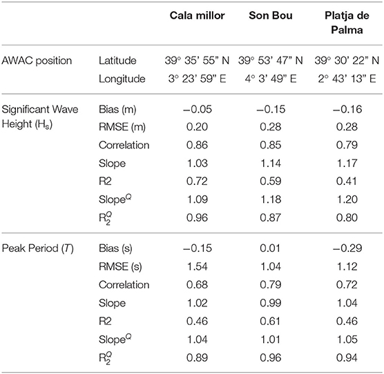
Table A1. Coordinates of the AWACs used for the validation of wave propagations and metrics resulting from the comparison between the instrumental and the propagated time series.

Pairs of simultaneous measured and synthetic H_s and T as well as the quantiles (q_n) associated with the percentiles (0,1,2,.,99,100) of each time series are considered to compute the following metrics:

$\begin{array}{ll}\text{Bias}=\overline{x^m}-\overline{x^s}& (\mathrm{A1})\end{array}$

$\begin{array}{ll}\text{RMSE}=\sqrt{\frac{1}{N}{\displaystyle \sum _{i=1}^N}{(x_i^m-x_i^s)}^2}& (\mathrm{A2})\end{array}$

$\begin{array}{ll}\text{Correlation}=\frac{{\displaystyle {\sum }_{i=1}^N}(x_i^s-\overline{x^s})(x_i^m-\overline{x^m})}{{\sigma }_{x^s}{\sigma }_{x^m}}& (\mathrm{A3})\end{array}$

$\begin{array}{ll}\text{Slope}=\frac{{\displaystyle {\sum }_{i=1}^N}{x}_i^s{x}_i^m}{{\displaystyle {\sum }_{i=1}^N}{x}_i^s{x}_i^s}& (\mathrm{A4})\end{array}$

$\begin{array}{ll}{\text{R}}_2=1-\frac{{\displaystyle {\sum }_{i=1}^N}{(x_i^m-x_i^s)}^2}{{\displaystyle {\sum }_{i=1}^N}{(x_i^m-\overline{x^m})}^2}& (\mathrm{A5})\end{array}$

$\begin{array}{ll}{\text{Slope}}^Q=\frac{{\displaystyle {\sum }_{n=1}^{101}}{q}_n^s{q}_n^m}{{\displaystyle {\sum }_{n=1}^{101}}{q}_n^s{q}_n^s}& (\mathrm{A6})\end{array}$

$\begin{array}{ll}{\text{R}}_2^Q=1-\frac{{\displaystyle {\sum }_{n=1}^{101}}{(q_n^m-q_n^s)}^2}{{\displaystyle {\sum }_{n=1}^{101}}{(q_n^m-\overline{q^m})}^2}& (\mathrm{A7})\end{array}$

where x symbolizes H_s or T; N is the number of time series samples considered for the analysis; $x_i^m$, $\overline{x^m}$ and ${\sigma }_{x^m}$ refer to the i^th sample, the mean and the standard deviation of the instrumental time series, respectively; while $x_i^s$, $\overline{x^s}$ and ${\sigma }_{x^s}$ refer to the i^th sample, the mean and the standard deviation of the synthetic time series, respectively. Also, $q_n^s$ and $q_n^m$ are the quantiles of the percentile n, for synthetic and measured time series, respectively (both for H_s and T); while $\overline{q^s}$ and $\overline{q^m}$ stand for the mean of the quantiles of the synthetic and measured time series, respectively. The results of the seven metrics described are listed in Table A1. Figure A1 shows scatter plots and QQ-plots for these data pairs.

FIGURE A1

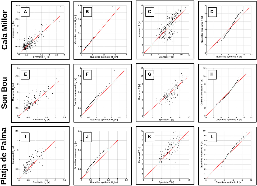
Figure A1. Comparison of in situ and synthetic time series (unitary slope lines indicated in red). (A,E,I) Show H_s scatter plots. (B,F,J) Show H_s QQ-plots. (C,G,K) Show T scatter plots. (D,H,L) Show T QQ-plots. (A–D) Correspond to Cala Millor data; (E–H) to Son Bou data; (I–L) to Platja de Palma data.

B. Justification of the Triangular Flooding Forcing

In order to define the form for the forcing of the temporary flooding, the WS + SS exceedances of all the flooding zones were considered. A prior visual inspection indicated that the shape of the exceedances tends to be triangular-like, at least at the sampling rate used.

A more quantitative analysis of the exceedances shape was conducted, consisting of the following. First, the time series were upsampled by a factor of 100 using linear interpolation, in order to capture the complete shape of each exceedance. Then, the exceedances were split in the rising and the falling parts (i.e., the part of the exceedances between the threshold up-crossing and the exceedance peak, and between the exceedance peak and the threshold down-crossing, respectively). The exceedance rises and falls were normalized to give values between zero and one, both in time and intensity. Later, the exceedance rises and falls were interpolated to a common grid, in order to compare the shape between all the exceedance rises and falls. Also, the ratios between the exceedance rise durations and the complete exceedance durations were computed.

The distribution of the exceedance rise and exceedance fall shapes, as well as the distribution of the ratio between the exceedance rise duration and the complete exceedance duration, are provided as Supplementary Material (“exceedance_shape_statistics.png”). The results shown in that image allow us to conclude that the most plausible shape for the temporary flooding (that indicated by the 50^th percentile) is somewhat more concave than a triangular pulse. Also, the histogram of the ratio between the exceedance rise duration and the complete exceedance duration indicates that the rise duration should be equal to the fall duration. Since the most plausible shape is close to a triangular shape, which is easier to generate and which has used before in the Literature (e.g., Purvis et al., 2008), we decided to use a triangular shape, with the same duration for the rise and the fall.

C. Synthetic Storm Surge and Significant Breaking Wave Height Time Series Generation

To characterize the statistics of H_b time series, it is necessary to consider the intensity of their samples, as well as the time distribution and persistence of storms, which in this case are defined as the events where the intensity of the forcing exceeds some threshold during a certain time, called persistence of the event (Toimil et al., 2017a). Once the statistics of the forcings are known, it is possible to generate synthetic time series that are statistically consistent with the original one, but with a different chronology, in this case based on Soares et al. (1996). These can be used to generate an estimation of the beach width time evolutions probability distribution, by means of a Monte Carlo method (by using Equation (7). We characterize the logarithm of H_b (clipped below -2) instead of H_b itself.

The forcing time series present annual stationarity. Thus, instead of characterizing the statistics of the whole time series, we classified their samples depending on their position inside the seasonal period and used the fragments of time series corresponding to each season (December, January, and February; March, April, and May; June, July, and August; September, October, and November).

For each group, we estimated its cumulative density function (CDF). For the logarithm of H_b we used a piecewise function with two intervals, where the range below the 99.9^th quantile was computed by linear interpolation, and the interval above that threshold was computed as 1 − (1 − 0.999) · (1 − CDF_GPD), where CDF_GPD is a Generalized Pareto distribution CDF, fitted by least squares.

Once the CDF of each group was estimated, we applied the inverse transformation method (Soares et al., 1996) to made each group's data follow a Gaussian distribution. Then, we computed and solved the Yule-Walker equations associated with each group's gaussianized data, obtaining an autoregressive filter for each group (Kay, 1993).

To obtain synthetic time series we generated Gaussian white noise and filtered it using the previously calibrated autoregressive filter (the output of the filter presents the same time correlation as the data used to calibrate the filter, though it follows a gaussian distribution). Afterward, the inverse transformation method was applied to obtain a time series presenting both the same time correlation and marginal distribution as the original data. Finally, in order to mimic the seasonality of the forcings, the filter and CDF of each season were switched periodically between the ones of the different groups. A comparison between the original and multiple synthesized time series for one beach is summarized in Figure A2 in the form of different statistics.

FIGURE A2

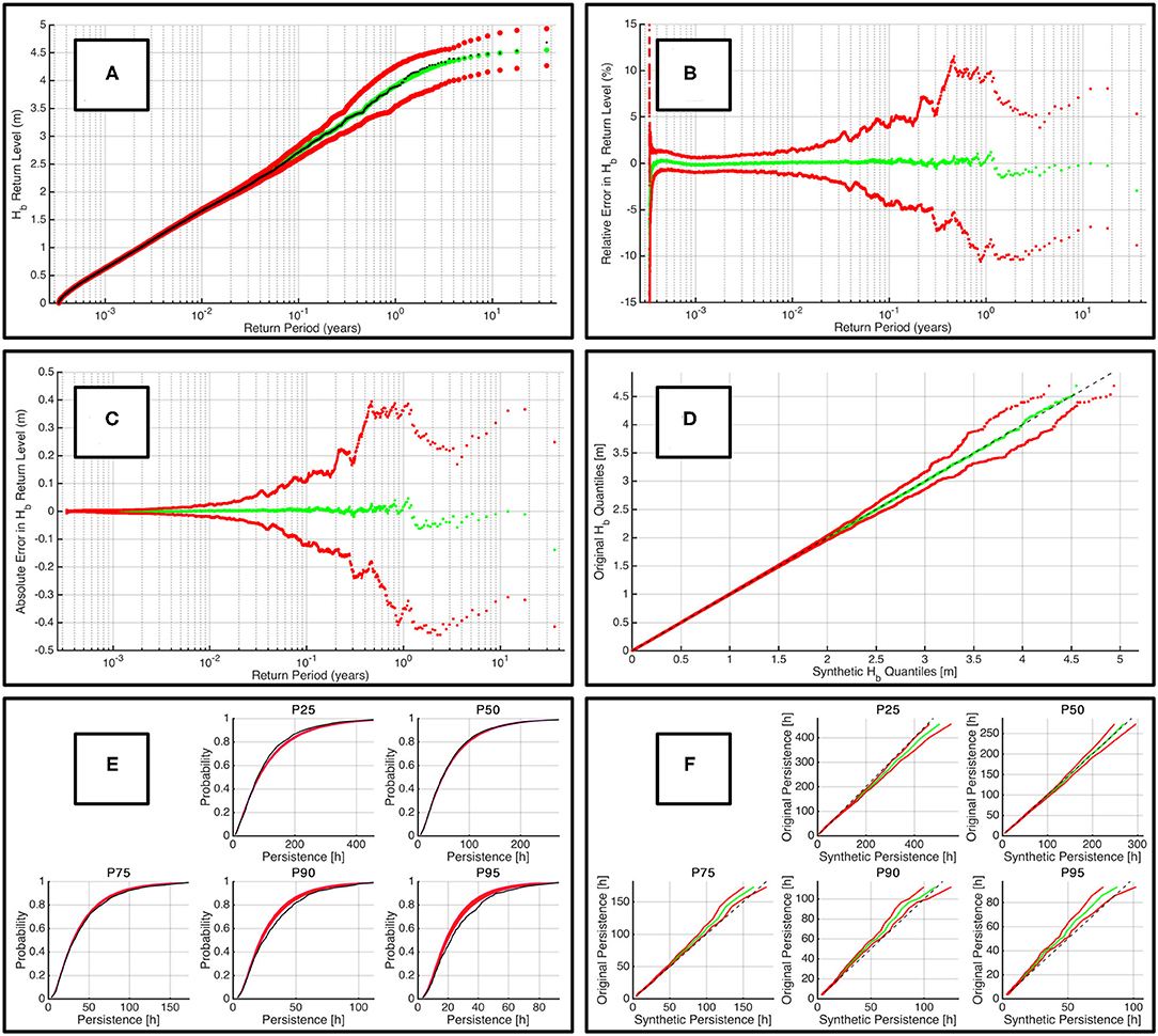
Figure A2. Comparison between the statistics of the original and 1000 synthetic time series of H_b for one beach. In all panels, black dots (or lines) indicate the values computed using the original time series; while the lower red dots, central green dots, and upper red dots (or lines) indicate the 5, 50, and 95th percentiles of the values computed from the synthetic time series. (A) Shows the return plots. (B) Shows the error of the synthetic time series return plots with respect to the original time series return plot, while (C) depicts the same but in terms of relative error. (D) Shows the QQ-plots between the original and the synthetic time series. (E) Shows the cumulative density functions of the persistence over different thresholds (defined as the original time series percentiles, marked above each subpanel), both for the original time series (black dots) and the range between the 5 and 95th percentiles of the synthetic time series (red shaded areas). (F) Shows the QQ-plots of the persistence over different thresholds (defined as the original time series percentiles) between the original and the synthetic time series.