 Lauriane Ribas-Deulofeu
 Pierre-Alexandre Château
 Vianney Denis
 Chaolun Allen Chen
- 1Biodiversity Research Center, Academia Sinica, Taipei, Taiwan
- 2Taiwan International Graduate Program-Biodiversity, Academia Sinica, Taipei, Taiwan
- 3Department of Life Science, National Taiwan Normal University, Taipei, Taiwan
- 4Department of Marine Environment and Engineering, National Sun Yat-sen University, Kaohsiung, Taiwan
- 5Institute of Oceanography, National Taiwan University, Taipei, Taiwan
- 6Department of Life Science, Tunghai University, Taichung, Taiwan
Structural complexity is an important feature to understand reef resilience abilities, through its role in mediating predator-prey interactions, regulating competition, and promoting recruitment. Most of the current methods used to measure reef structural complexity fail to quantify the contributions of fine and coarse scales of rugosity simultaneously, while other methods require heavy data computation. In this study, we propose estimating reef structural complexity based on high-resolution depth profiles to quantify the contributions of both fine and coarse rugosities. We adapted the root mean square of the deviation from the assessed surface profile (Rq) with polynomials. The efficiency of the proposed method was tested on nine theoretical cases and 50 in situ transects from South Taiwan, and compared to both the chain method and the visual rugosity index commonly employed to characterize reef structural complexity. The Rq indices proposed as rugosity estimators in this study consider multiple levels of reef rugosity, which the chain method and the visual rugosity index fail to apprehend. Furthermore, relationships were found between Rq scores and specific functional groups in the benthic community. Indeed, the fine scale rugosity of the South Taiwan reefs mainly comes from biotic components such as hard corals, while their coarse scale rugosity is essentially provided by the topographic variations that reflect the geological context of the reefs. This approach allows identifying the component of the rugosity that could be managed and which could, ultimately, improve strategies designed for conservation.
Introduction
Climate Change and Its Impacts on Reef Structural Complexity
Climate change and anthropogenic pressures transform ecosystems and jeopardize the services they provide, especially in coral reefs (Vergés et al., 2014; Hughes et al., 2017; Pecl et al., 2017). Coral reefs are affected from the physiological to ecosystem levels (Pendleton et al., 2016; Richmond et al., 2018) by increasing sea surface temperatures (SST), ocean acidification, and typhoons, along with a plethora of additional anthropogenic threats (Wilkinson, 1999; Hoegh-Guldberg et al., 2007; Carpenter et al., 2008; Carilli et al., 2009; Rogers et al., 2014; Darling et al., 2019; Ribas-Deulofeu et al., 2021). Reefs must show increasing capacities to resist and recover from stressors in order to persist (Hughes et al., 2003, 2010, 2011). In this context, structural complexity has been identified as a critical factor to understand reef resilience abilities (Graham et al., 2015; Maynard et al., 2017). A growing body of literature on reef rugosity has highlighted the losses in reefs’ structural complexities together with an erosion of resilience capacities (Syms and Jones, 2000; Chong-Seng et al., 2012; Graham and Nash, 2013; González-Rivero et al., 2014; Rogers et al., 2014). Mechanical damages and reduced growth rates of corals have led to a consequential loss in reef structural complexity over the past decades (Young et al., 2012; Bozec et al., 2015; Hoegh-Guldberg et al., 2017; Mollica et al., 2018).
Historical Background on Reef Rugosity Investigations
Measurements of reef structural complexity were first performed by Risk in the 1970s (Risk, 1972), and were later adapted by Luckhurst and Luckhurst (1978) into the “rugosity index,” also referred to as the chain method, which measures the difference between the distance covered by a fine-link chain closely laid over a substrate and its known linear distance. Since then, the rugosity parameter has remained the most widely used measure of reef structural complexity, and multiple methods to estimate it have been proposed (e.g., Polunin and Roberts, 1993; Dustan et al., 2013; Young et al., 2017; Lazarus and Belmaker, 2021). In the 1990s, the visual rugosity index emerged to estimate larger scales of rugosity (Polunin and Roberts, 1993). This proposed index was based on a six-point scale ranging from zero—no vertical relief observed along the transect—to five—an exceptionally complex substrate relief with numerous caves and overhangs characterizing the transect (Polunin and Roberts, 1993; Wilson et al., 2007).
Since then, improvements in underwater techniques and other technological advances have allowed researchers to develop new methods and metrics to assess reef rugosity more accurately (Figueira et al., 2015; Ferrari et al., 2016; Young et al., 2017; Lazarus and Belmaker, 2021). Yet, even with enhanced tridimensional models, most of the recent studies have used linear-rugosity (chain method) or fractal dimensions to quantify reef rugosity (Ferrari et al., 2016; Young et al., 2017; Magel et al., 2019). In addition, most recent methods have been impeded by either their restricted resolution (e.g., satellite imagery) or their operational capacities in underwater ecosystems (e.g., Structure from Motion (SfM) photogrammetry), reducing the range of reefs in which researchers could implement them (Friedman et al., 2012; Knudby et al., 2014; Burns et al., 2015; Figueira et al., 2015; Ferrari et al., 2016; Yanovski et al., 2017). On the other hand, despite the broad acceptance of the traditional chain method, its in situ deployment remains laborious, time consuming, and inaccurate compared to techniques such as SfM photogrammetry (Risk, 1972; Luckhurst and Luckhurst, 1978; Knudby and LeDrew, 2007). In parallel, visual estimations of habitat complexity (Polunin and Roberts, 1993) have been widely used and praised for their correlations with the fish communities (Wilson et al., 2007). However, visual census approaches show limited relationships with benthic composition and yield observer bias, making the studies that use them difficult to replicate (Bayley et al., 2019). The more recent development of the Digital Reef Rugosity (DRR) method by Dustan et al. (2013) offers a good compromise between data resolution and field implementation difficulties. Yet, as suggested by the authors themselves, other statistics on depth profiles might yield better rugosity estimations than what they proposed (Dustan et al., 2013). Consequently, none of the existing methods or metrics led to a consensus on how reef rugosity should be measured or estimated (Knudby and LeDrew, 2007; Graham and Nash, 2013; Yanovski et al., 2017; Lazarus and Belmaker, 2021).
The Influence of Types of Rugosity on Ecosystem Functioning
Coral reef rugosity is based essentially on the physical characteristics of the inhabiting organisms, and this structure can be measured from the micro scale (from millimeters to decimeters) to the macro scale (e.g., based on larger organisms such as massive Porites colonies, which can reach over a meter in scale) (Graham and Nash, 2013; Darling et al., 2017). In addition, the geological context of the studied reef also contributes to its rugosity, especially to its macro-rugosity (Kleypas et al., 2001; Graham and Nash, 2013; Darling et al., 2017). Numerous fish and other mobile reef organisms have been shown to prefer specific structural scales (Chong-Seng et al., 2012; Graham and Nash, 2013; Richardson et al., 2017). In the Indo-Pacific, studies showed that micro-rugosity, such as that provided by branching corals, tends to favor smaller fishes, such as Pomacentridae, as it offers them many potential refuges (e.g., Wilson et al., 2008; Graham and Nash, 2013), while large and medium-sized fishes show stronger relationships with macro-rugosity (Wilson et al., 2008; Dustan et al., 2013). Consequently, it is crucial to quantify the contributions of the different scales of rugosity to the overall reef rugosity, along with the contributions from biotic (reef organisms) and abiotic (geological features) parameters, since reef organisms constitute the primary targets of management strategies (Harborne et al., 2012; Graham et al., 2015; Darling et al., 2017). The chain method and SfM photogrammetry describe the finer scale of habitat variability (Knudby and LeDrew, 2007; Dustan et al., 2013; Magel et al., 2019) and most remote-sensing methods describe larger scale factors such as bathymetric variations (Purkis et al., 2008; Friedman et al., 2012; Dustan et al., 2013; Graham and Nash, 2013). Missing finer- or broader-scale rugosities may result in only a partial understanding of the relationship between structural complexity and reef composition and, ultimately, lead to inadequate reef management strategies (Friedman et al., 2012; Graham et al., 2015; Maynard et al., 2017).
Consequently, in this study, we propose a framework that combines fine-scale depth profiles with fast computations to accurately quantify reef rugosity, but more importantly to measure the relative contributions of fine and coarse rugosities (decimeter to meters) into the overall rugosity of the reef ecosystems. We present nine theoretical cases to demonstrate our method. We further tested the feasibility and performance of our method on 50 fine-scale depth profiles from South Taiwan coral reefs.
Materials and Methods
Rugosity Estimations
Reef rugosity estimations were based on high-resolution depth profiles from theoretical and in situ line-transects. Our calculations (Supplementary File 1) used the roughness index Rq, developed for engineering purposes to estimate the surface roughness profile of materials (Posey, 1946). Rq (also called R.M.S. in certain studies) represents the Root Mean Squared deviation from the assessed surface profile. To discriminate between the contributions of fine and coarse scales of rugosity on the total rugosity profile, we adapted the Rq index (Equation 1) as followed:
with l = ; in this study, l = 20m.
Rugosity profiles were then plotted along with a first-degree polynomial function to represent the total rugosity of each transect (fine and coarse scales rugosity, Rq1). Successive estimations of Rq were performed from the first order of polynomial up to the twelfth order. As the orders of polynomials increased, the fit we obtained improved, and thus the remaining rugosity decreased, allowing us to move along a continuum from coarse to fine scale rugosity. Rq1 represents the overall rugosity of our line-transects, while Rq12 corresponds to the fine scale rugosity contribution. To estimate the proportion of coarse scale rugosity in our transects, we subtracted the fine scale rugosity Rq12 from the overall rugosity Rq1 of the transect. From here on, we refer to the contribution of coarse scale rugosity to the transects as Rq1–Rq12.
To compare our method with commonly used rugosity methods, we computed the expected rugosity of our transects with the chain method. Our “virtual chain index” (Equation 2) was calculated as followed:
with virtual chain link size corresponding to the depth profile resolution of the transects, since .
In addition, to mimic diving conditions, two observers used videos to visually categorize the structural complexity of our in situ transects using the six-point scale proposed by Polunin and Roberts (1993). Zero, the first level, corresponded to no vertical relief observed along the transect. Levels one and two corresponded to sites with low structural complexity, and sparse and widespread relief, respectively. Level three was for moderately complex sites, while level four was for very complex sites with numerous caves and fissures. Finally, level five corresponded to sites with exceptional complexity, including numerous caves and overhangs (Polunin and Roberts, 1993; Wilson et al., 2007).
Datasets
Theoretical Cases
To demonstrate our method, nine 20-m long theoretical transects were generated (Supplementary File 2). Resolution between two depth measurements on our theoretical cases was set to 12.50 cm. Three levels of coarse scale rugosity were defined: low for the transects Theo1, Theo2, and Theo3; medium for Theo4, Theo5, and Theo6; and high for Theo7, Theo8, and Theo9 (Figure 1). Three levels of fine scale rugosity were also defined to represent all possible combinations of fine and coarse scale rugosity levels. Indeed, Theo1, Theo4, and Theo7 were classified as low fine scale rugosity; Theo2, Theo5, and Theo8 as medium fine scale rugosity; and Theo3, Theo6, and Theo9 as high fine scale rugosity (Figure 1). The nine theoretical transects defined in this study allowed us to test how well our rugosity indices discriminated transects with known gradients of fine and coarse scale rugosity (Figure 1).
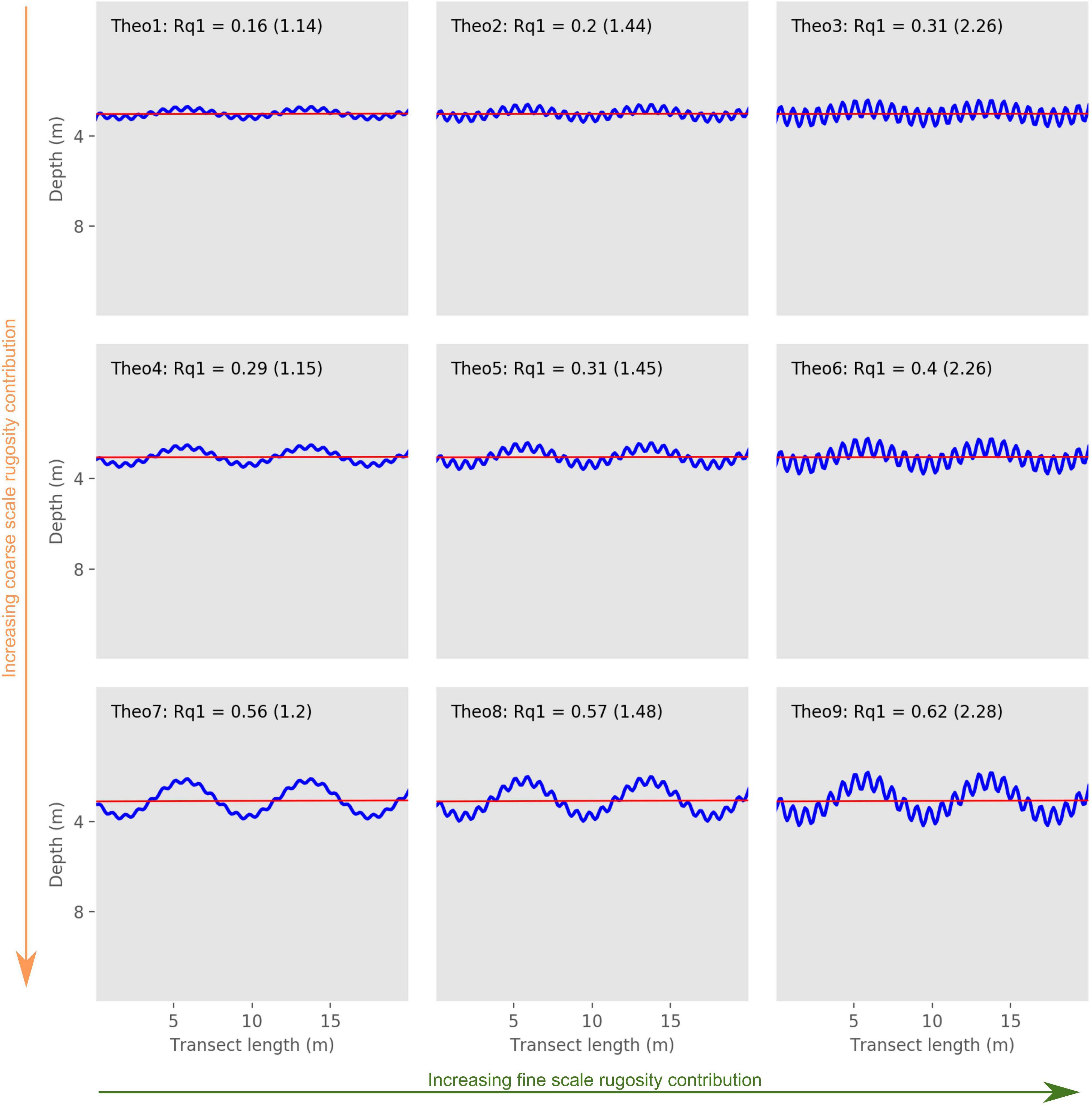
Figure 1. Theoretical depth profiles. Rows and columns represent cases with the same level of coarse and fine scale rugosity, respectively. The orange and green arrows represent the increasing gradient of coarse and fine scale rugosity, respectively. The blue lines represent the actual depth profiles of the nine theoretical transects and the red lines represent the first order of polynomial. Rq1 value is reported for each transect, along with its chain index score in parentheses.
Field Survey
Fifty field transects were surveyed at 10 locations (Supplementary File 3) in Kenting National Park (KNP), at the southern tip of Taiwan (21.90°N, 120.79°E), to test the performances of our method (Figure 2 and Table 1). Transects were positioned around 5 m in depth, with a minimum depth of 1.8 m and a maximum one of 10.1 m. The field data presented in this study were collected in July and August 2015.
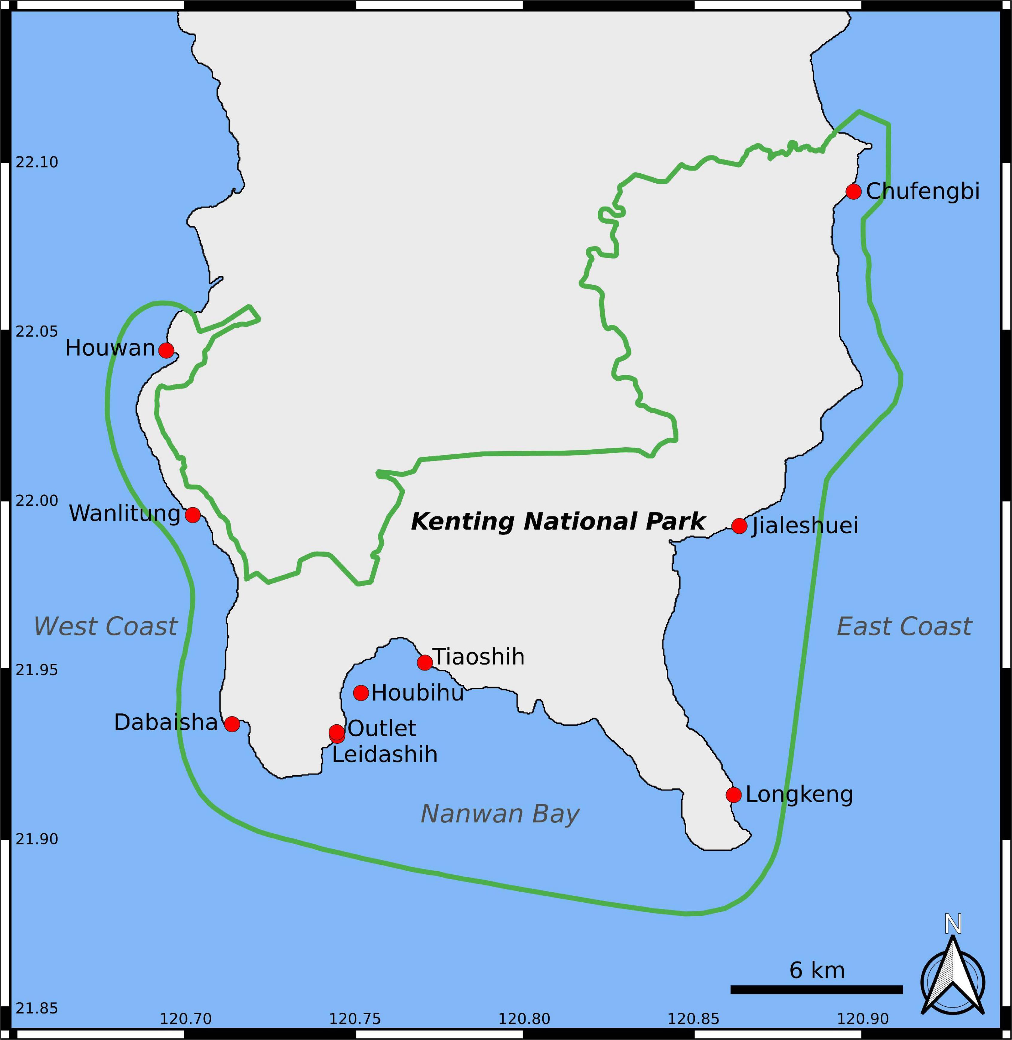
Figure 2. Study area. Green line represents the limits of KNP, while red dots represent surveyed sites.
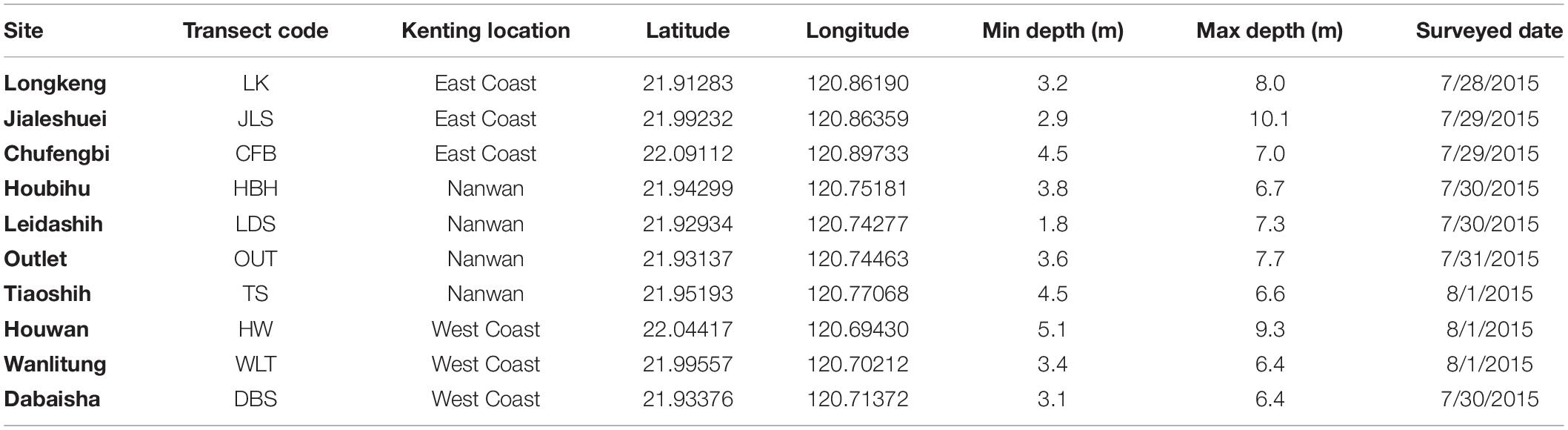
Table 1. Information on the locations surveyed.
Fine resolution depth profiles were recorded following the method proposed by Dustan et al. (2013). At each site, water pressure data along five 20-m-long line transects was measured using a titanium HOBO water level logger (U20-001-03-TI) pre-programmed to start at the specific hour of the onset of our surveys. In our case, pressure records were set at 2-s intervals to sustain battery life for survey of 10 sites. For reference, with temperature disabled, the logger offers up to 50 h of continuous recording. According to the focus of the survey (individuals, communities, seascape), we would recommend to adjust measurement interval to capture the resolution of interest (here colony scale—decimeter). Once set, barometric pressure variations were recorded pre-dive at sea-level for over 5 min. Wave height variations were estimated by keeping the logger still at the sea-bottom for 2–4 min, as recommended by Dustan et al. (2013). To record the actual transect depth profile, the diver progressed slowly at a constant horizontal speed along the transect following as closely as possible, but carefully, the reef topography, while paying extra attention to not damage the reef (Dustan et al., 2013).
Starting and ending times of sea-level and sea-bottom recordings along with the beginning and end times of each transect recordings were noted. In addition, time synchronization between diving computer and the computer used to download the data from the logger were checked prior to the field survey, in order to accurately identify and subset the useful data from the raw file extracted from the logger (Dustan et al., 2013). Pressure data were subset by transect and converted into depth profiles using the formula recommended by Fofonoff and Millard (1983). Their formula (Equation 3) resolves the inconsistency in the pressure/depth conversion caused by gravitational variations through latitudinal and depth gradients (Fofonoff and Millard, 1983), allowing our technique to be replicated at any location or depth around the globe.
with p (pressure) measured in decibars (hPa/10) and .
The resolution of the 50 depth profiles was one measurement every 15.73 ± 1.50 cm on average. The lowest resolution for those profiles was one measurement every 19.41 cm (LK3 on the East Coast) and the highest was one measurement every 12.58 cm (HBH4 in Nanwan).
Rugosity indices were calculated for both theoretical and in situ transects. To identify transects with similar rugosity patterns, principal component analyses (PCA) using the overall, fine and coarse scale rugosity indices (Rq1, Rq12 along with Rq1–Rq12) were performed on the 50 surveyed transects and the nine theoretical ones. Rq indices and Rq1–Rq12 were standardized prior to the PCA.
Relationships Between Rugosity Patterns and Benthic Composition
Benthic composition data were collected along the same transects as the field rugosity data. Photo-quadrats (0.5 m × 0.5 m) were captured every meter along the 20-m-long line transects following the method described in Ribas-Deulofeu et al. (2016). In each photograph (50 random points/photograph), the benthic organisms were identified using 133 Operational Taxonomic Units (OTUs), in the CPCe v4.0 software (Kohler and Gill, 2006). The detailed benthic dataset is available in Ribas-Deulofeu et al. (2021). The relationships between rugosity patterns (Rq1, Rq12, and Rq1–Rq12) and benthic composition were investigated using transformation-based redundancy analysis (tb-RDA) (Legendre and Legendre, 2012). Tb-RDA analysis was performed on Hellinger-transformed benthic cover, while rugosity indices were standardized. In the benthic composition dataset, the major categories that contributed to less than 5% in any transect were excluded in the tb-RDA analysis (McCune and Grace, 2002). Collinearity between the remaining 12 benthic categories was tested using the variance-inflation factors. Variables scoring over 10 (Borcard et al., 2018) in the variance-inflation factors of variables were excluded from the tb-RDA analysis.
All data were analyzed in Python (2.7) and R (v3.5.1) using packages vegan (Oksanen, 2018) and ggvegan (functions available at https://github.com/gavinsimpson/ggvegan/).
Results
Rq1, Rq12, and Rq1–Rq12 Performances
Theoretical Cases
Rq1 was lowest for Theo1 (0.16), which is consistent with the characteristic established for our theoretical transects, as Theo1 had the lowest coarse and fine scale rugosity levels, and consequently the lowest overall rugosity (Figure 1 and Table 2). On the other hand, Theo9 had the highest Rq1 score (0.62), which is also consistent with the theoretical transects characteristics, as this transect represents the highest level of coarse and fine scale rugosity and is consequently expected to represent the highest overall rugosity among our theoretical transects (Figure 1 and Table 2). Theo1, Theo4, and Theo7 had the lowest Rq12 score (0.07), as they are characterized by the lowest fine scale rugosity level, while Theo3, Theo6, and Theo9 had the highest Rq12 score (0.28), as they represented the highest level of fine scale rugosity in our theoretical set (Figure 3 and Table 2). The coarse scale rugosity gradient was also confirmed by our Rq1–Rq12 index: Theo1, Theo2, and Theo3 had the lowest score (0.03–0.08); Theo4, Theo5, and Theo6 had an intermediary score (0.11–0.21); and Theo7, Theo8, and Theo9 had the highest score (0.34–0.49; Figure 1 and Table 2).
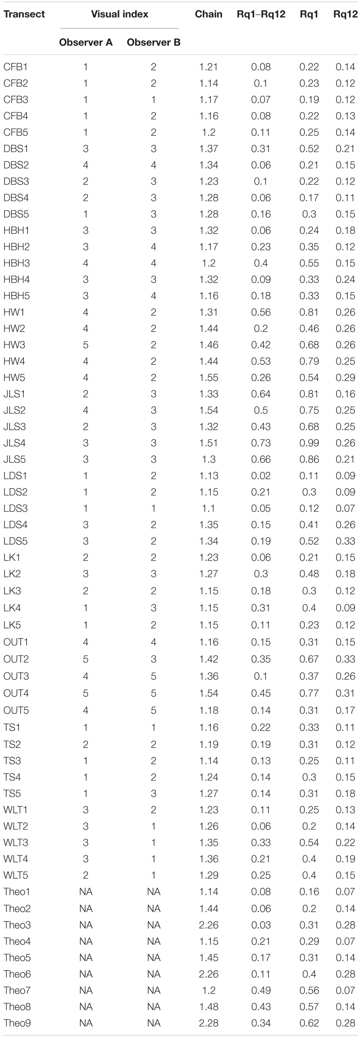
Table 2. Rugosity indices for all theoretical and in situ transects.
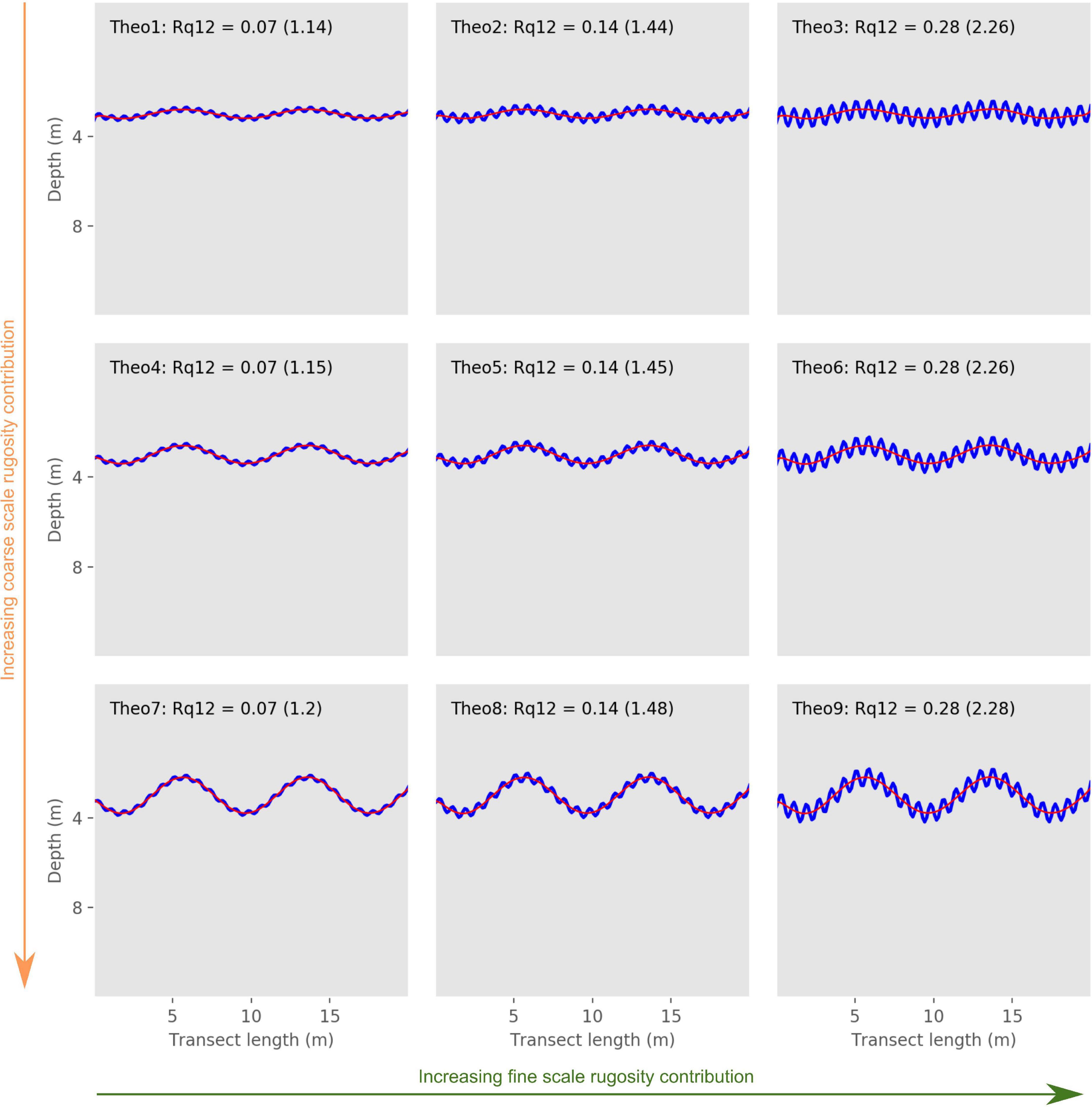
Figure 3. Depth profiles of the theoretical transects along with their twelfth order of polynomial. Elevation profiles (blue lines) for each transect. Red lines represent the twelfth order polynomials. Chain index results are reported in parentheses; the orange and green arrows represent the increasing gradients of coarse and fine scale rugosity, respectively, between transects.
Our Rq12 and Rq1–Rq12 indices correctly estimated the coarse and fine scale rugosity gradients established for our theoretical transects (Figures 1, 3, Table 2, and Supplementary Figure 1). Rq1 allowed us to compare transects with different levels of coarse and fine scale rugosity and surmise which cases represent high overall rugosity.
In situ Cases
Horizontally, intervals between two depth measurements in the in situ transects ranged from 12.58 cm (HBH4) to 19.41 cm (LK3). Vertically, the minimum and maximum deviations observed between the depth profiles and their fitted polynomial functions were 0.00 cm (twelfth-degree polynomial, CFB2), and 227.56 cm (first-degree polynomial, JLS4), respectively.
The highest Rq1 scores were observed in JLS4 (0.99), followed by JLS5 (0.86) and HW1 and JLS1 (0.81 for both) (Figure 4, Table 2, and Supplementary Figure 2). These transects presented the highest Rq1–Rq12 scores (0.56–0.73). However, while they did not have the highest Rq12, they did score fairly high (0.16–0.26, Figure 5, Table 2, and Supplementary Figure 2). Among the entire data set, the four highest Rq12 scores were 0.29–0.33.
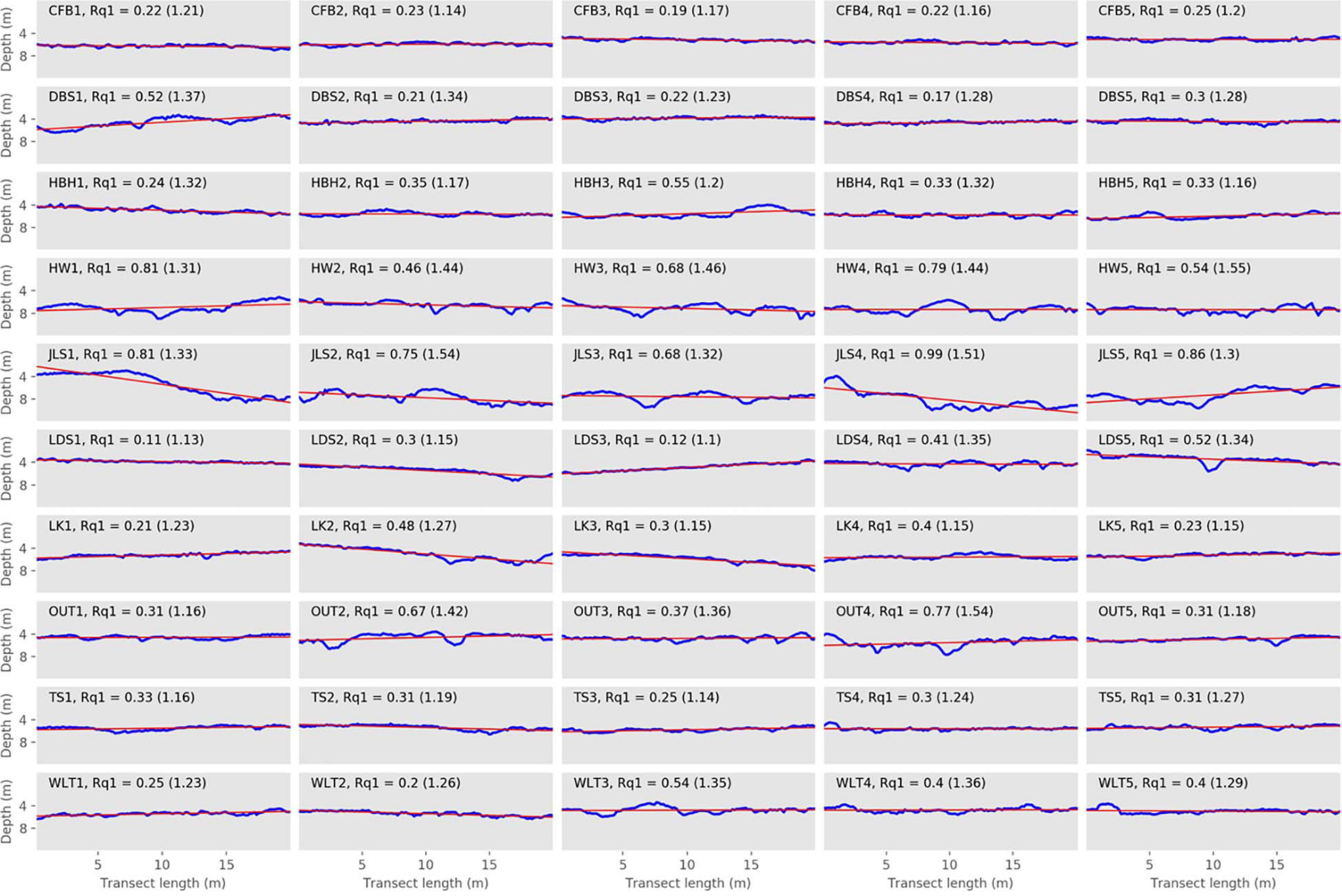
Figure 4. Depth profiles of the surveyed transects along with their first order of polynomial. Elevation profiles (blue lines) for each transect from the 10 surveyed sites in 2015. Red lines represent the first order polynomials. Chain index results are reported in parentheses.
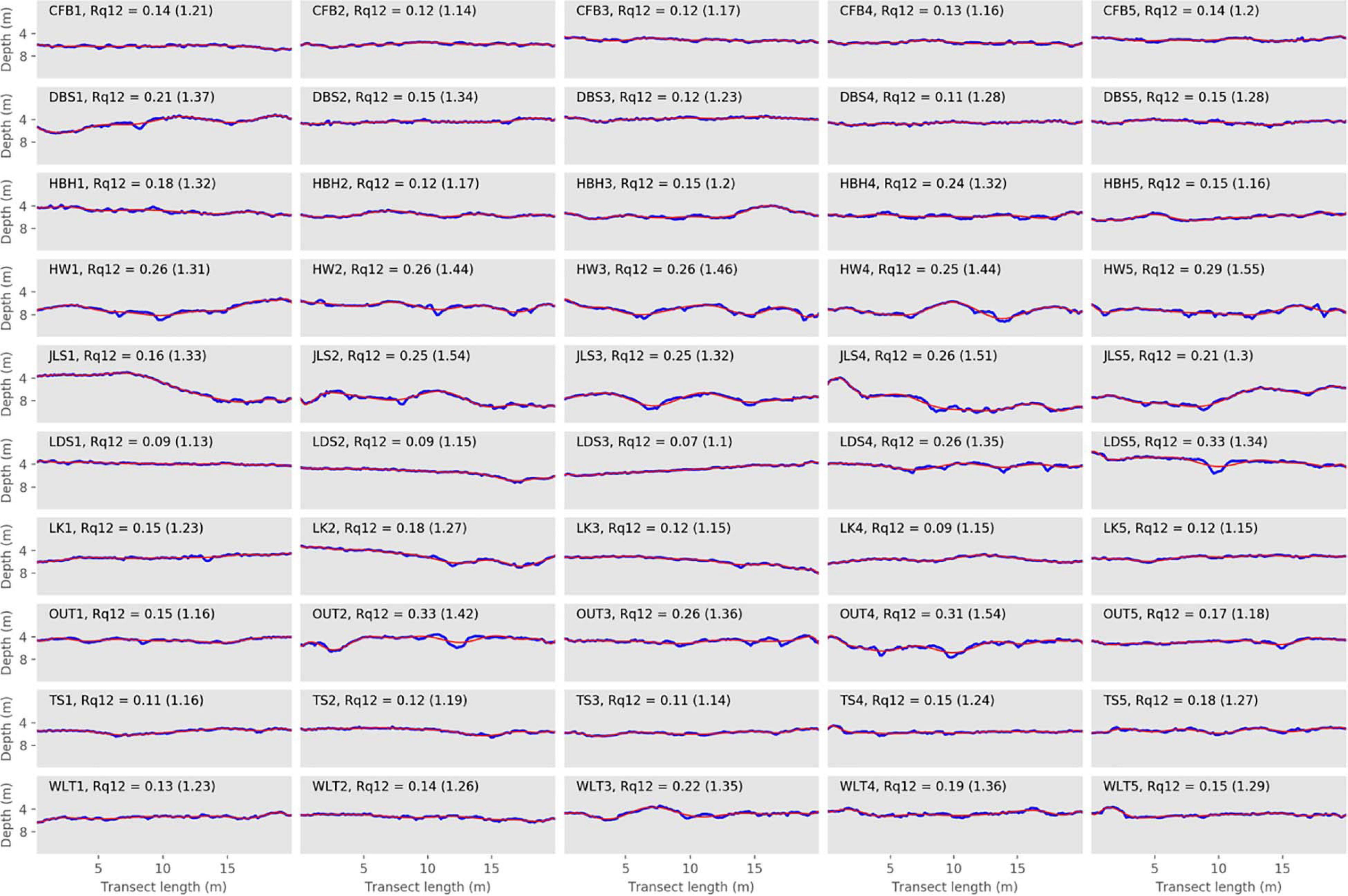
Figure 5. Depth profiles of the surveyed transects along with their twelfth order of polynomial. Elevation profiles (blue lines) for each transect from the 10 surveyed sites in 2015. Red lines represent the twelfth order polynomials. Chain index results are reported in parentheses.
On the other hand, the lowest Rq1 occurred in LDS1 (0.11), LDS3 (0.12), DBS4 (0.17), and CFB3 (0.19) (Figure 4 and Table 2). LDS1, LDS3, and DBS4 were also among the transects with the lowest Rq1–Rq12 (0.02, 0.06, and 0.7, respectively), along with DBS2, HBH1, LK1, and WLT2 (0.06 for each). Furthermore, three of these transects—LDS3, LDS1, and DBS4—also presented the lowest Rq12 observed among our field transects (0.07, 0.09, and 0.11, respectively); LK4 and LDS2 (0.09 for both) and TS1 and TS3 Rq12 scores were equal to DBS4 (0.11) (Figure 5, Table 2, and Supplementary Figure 2).
Comparison With the Chain Index
Theoretical Cases
Our theoretical transects had chain index values between 1.14 and 2.28 (Table 2). The chain index was lowest for the transect Theo1 (1.14), which was the theoretical case in our theoretical transects with the lowest overall rugosity and low coarse and fine scale rugosity levels (Figure 2). In addition, the chain index was indeed the highest for our Theo9 case, which had the highest overall rugosity and high coarse and fine scale rugosity levels (Figure 1 and Table 2). However, increases in chain index values were negligible when coarse scale rugosity proportions were increased between transects (e.g., 1.14 for Theo1, 1.15 for Theo4, and 1.2 for Theo7, where Theo1, Theo4, and Theo7 are characterized by the same fine scale rugosity but an increasing coarse scale rugosity). This highlighted the poor ability of the chain index to capture coarse scale rugosity (due to small chain link size), whereas chain index scores increased with increasing fine scale rugosity levels (e.g., 1.14 for Theo1, 1.44 for Theo2, and 2.26 for Theo3, where Theo1, Theo2, and Theo3 are characterized by the same coarse scale rugosity but increasing fine scale rugosities).
In situ Cases
For the transects scoring the same chain index with at least one other transect (34 transects), 79.4% of them (27 transects) showed different rugosity patterns (Table 2). For example, LDS5 and DBS2 were both 1.34. However, these two presented very different Rq1, Rq1–Rq12, and Rq12 (Figures 4, 5 and Table 2). Indeed, their Rq1 values were 0.52 and 0.21, Rq1–Rq12 were 0.19 and 0.06, and Rq12 were 0.33 and 0.15, respectively. A similar situation was observed with HW2 and HW4 (Figures 4, 5 and Table 2): although their chain index scores were the same (1.44) and Rq12 values were very similar (0.26 and 0.25, respectively), the two transects showed different Rq1–Rq12 levels, with HW4 (0.53) having more than twice the value as HW2 (0.20). This, in turn, resulted in a large difference in the two’s Rq1 values (0.46 and 0.79, respectively).
Comparison With the Visual Rugosity Index
The visual rugosity index has been estimated for the 50 in situ transects by two observers. The observers only agreed on rugosity estimations for 16 of these transects. For most transects (22 out of 50), their rugosity estimations only differed by 1 level (e.g., 4 of the 5 transects from Chufengbi were ranked level 1 by one observer and level 2 by the other). For 12 of the 50 transects, the estimations differed by at least 2 levels (e.g., WLT2 to WLT4 were ranked level 3 by one observer and level 1 by the other). The greatest difference between the observers was 3 levels.
There was variability in the chain index and Rq indices among transects that had equal visual rugosity index scores. For example, the chain indices of the six transects ranked level 3 by both observers (DBS1, HBH1, HBH4, JLS4, JLS5, and LK2) ranged from 1.27 to 1.51. Similarly, for these transects, Rq1 ranged from 0.24 to 0.99, Rq1–Rq12 ranged from 0.06 to 0.73, and Rq12 ranged from 0.18 to 0.26.
Multivariate Analysis of Rugosity Indices
Theoretical Cases
The first axis (PCA1, 56.19% of the variance explained) of the PCA based on the theoretical transects only (n = 9) mainly represented the fine scale rugosity gradient, as Rq12 was −0.99 (Figure 6, note that in the figure, inverse of PCA1 and PCA2 are used for visualization purpose), while Rq1 was −0.16 and Rq1–Rq12 was 0.47. The second axis (PCA2; 43.81%) mainly represented the overall rugosity and coarse scale rugosity gradient, with Rq1 and Rq1–Rq12 of −1.62 and −1.04, respectively, and a Rq12 of −0.22 (Figure 6). Pearson correlation tests were performed between variables. Rq1–Rq12 and Rq1 showed strong correlation [r(7) = 0.85, p-value = 0.004]. However, Rq1 and Rq12, as well as, Rq1–Rq12 and Rq12 showed moderate, but non-significant, correlations [r(7) = 0.29, p-value = 0.44, and r(7) = −0.26, p-value = 0.5, respectively].
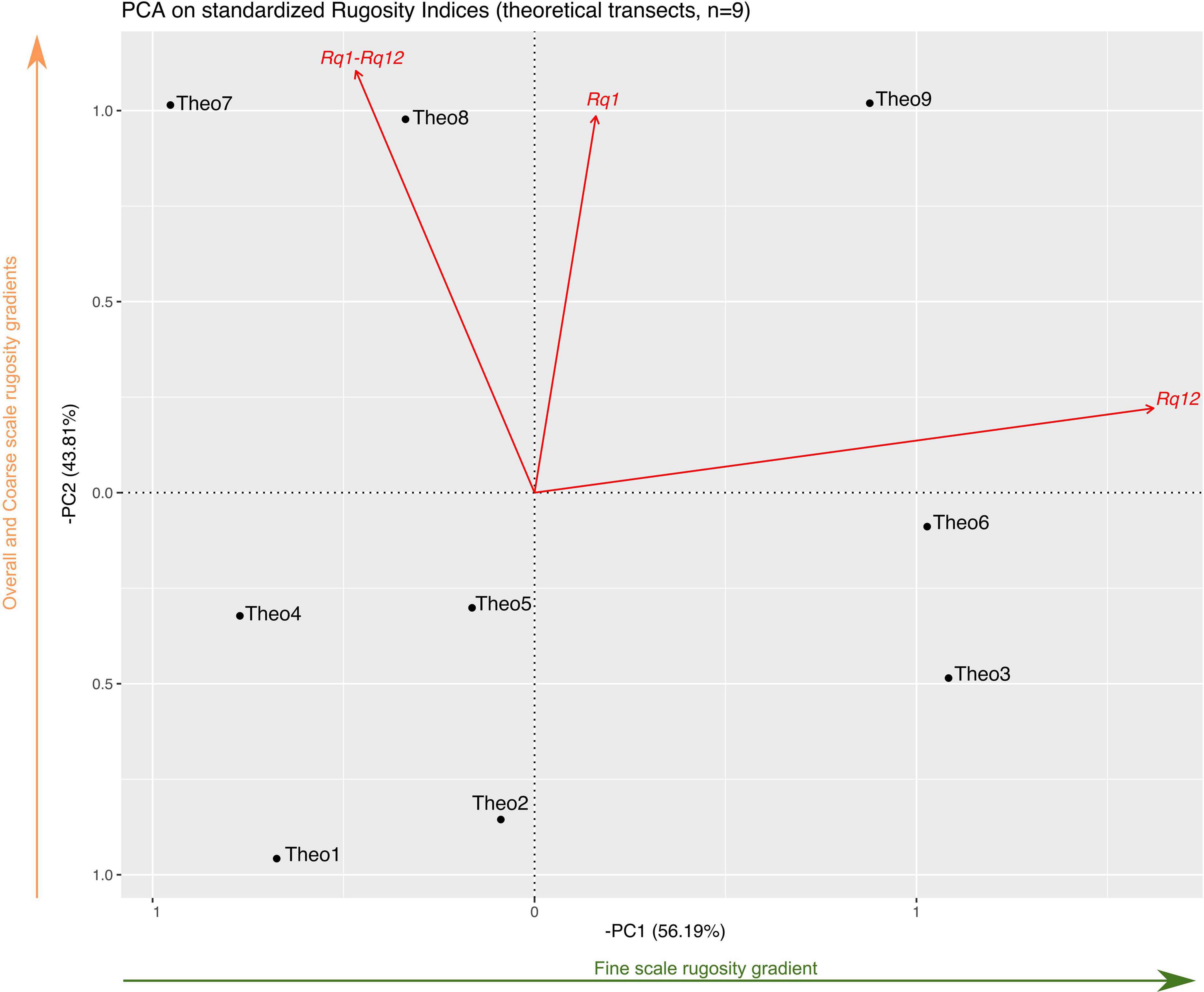
Figure 6. PCA representation of rugosity indices for the nine theoretical transects. PCA axes are displayed as their inverse to better visualize rugosity gradients; this did not influence the relative position between transects. Scores reported in the text are the exact scores obtained by the PCA analysis without inversion of the x- and y-axes. Red arrows represent the variables’ vectors, the green arrow under the x-axis illustrates the fine scale rugosity gradient between transects, and the orange arrow beside the y-axis represents the overall and coarse scale rugosity gradients.
Rugosity gradients were well illustrated by the position of the theoretical transects in the PCA (Figure 6). Transects with the same Rq12 but increasing Rq1–Rq12 followed increasing gradients along PCA2 (from Theo1 to Theo4 and Theo7, Theo2 to Theo5 and Theo8, and Theo3 to Theo6 and Theo9; these three transect trios are characterized by the same respective Rq12). On the other hand, transects with similar Rq1–Rq12 but increasing Rq12 (Theo1 with Theo2 and Theo3, Theo4 with Theo5 and Theo6, and Theo7 with Theo8 and Theo9) followed an increasing gradient of Rq12, as PCA1 is mainly explained by fine scale rugosity (Figure 6).
In situ Cases
The first axis of the PCA (PCA1, 83.64% of the variance explained) considering only the in situ transects (n = 50) mainly represented the overall-rugosity gradient, as Rq1 was 2.08 (Figure 7), Rq12 was 1.48, and Rq1–Rq12 was 1.91. The second axis (PCA2; 16.36%) mainly represented the opposing coarse and fine scale rugosity gradients, with Rq12 and Rq1–Rq12 scoring −1.20 and 0.72, respectively, and Rq1 scoring 0.19 (Figure 7). Note that Rq1–Rq12 and Rq1 were strongly correlated [Pearson correlation: r(48) = 0.96, p-value <0.001], Rq1 and Rq12 showed high correlation [r(48) = 0.72, p-value < 0.001], and a moderate correlation was found between Rq1–Rq12 and Rq12 [r(48) = 0.51, p-value < 0.001].
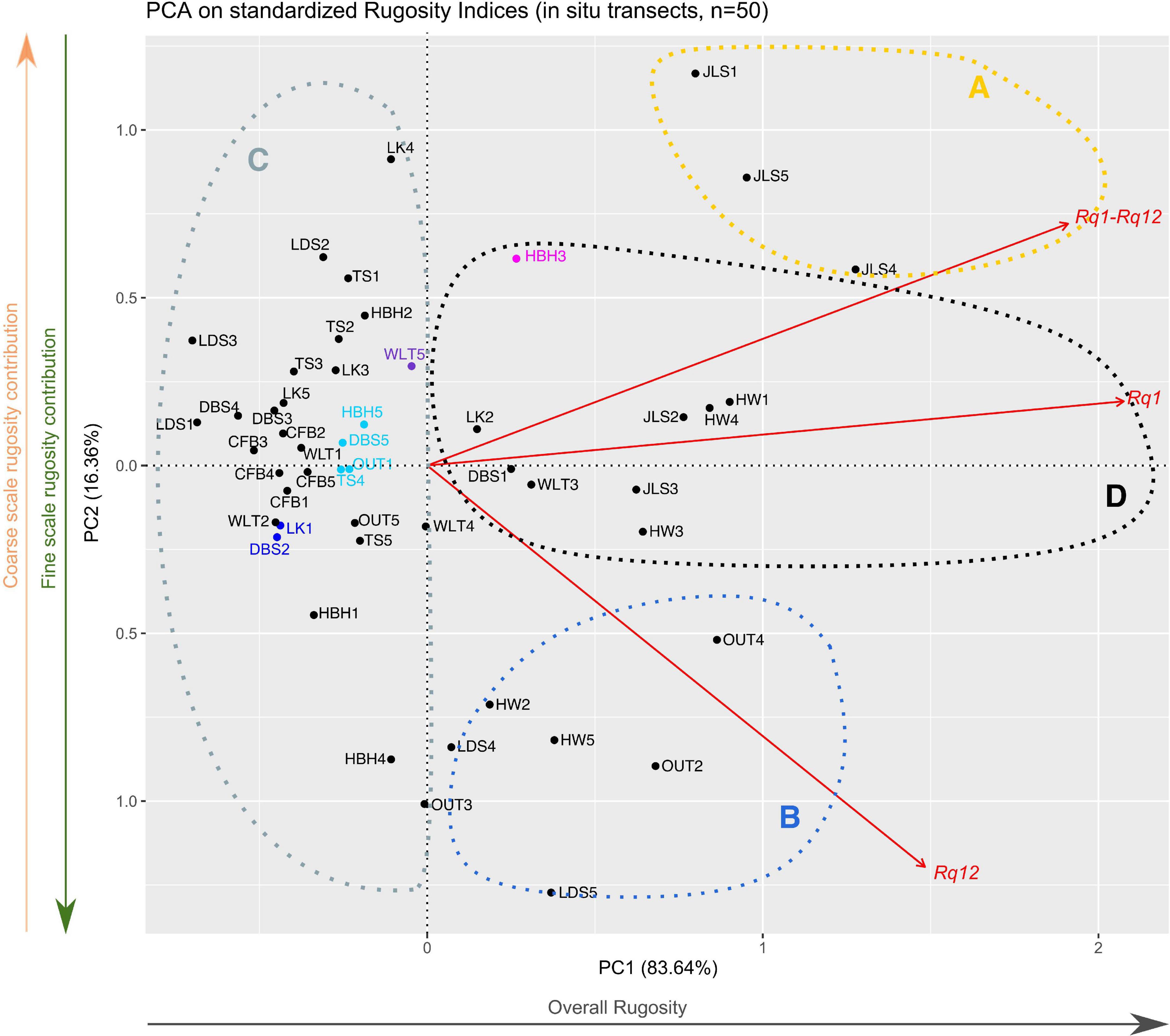
Figure 7. PCA representation of rugosity indices for the 50 in situ ones. Red vectors represent the contribution of the rugosity indices to the PCA, while black and colored dots represented the transects used in this study. The eight colored dots (navy blue, cyan, purple, and fuchsia) represent transects that were used as examples in the “Results” section (Importance of Using Multiple Rugosity Indices and Distinguishing Among Types of Rugosity). The gray arrow under the x-axis illustrates the overall rugosity gradient between transects, while the green and orange arrows besides the y-axis represented the fine and coarse scale rugosity gradients, respectively. Dashed circles represent the proposed target transects used to illustrate potential management strategies in the discussion.
Importance of Using Multiple Rugosity Indices and Distinguishing Among Types of Rugosity
In our set of in situ transects, some presented equal Rq scores for a given polynomial level. However, those same transects showed different patterns when depth profiles or other Rq levels were investigated. To illustrate this type of situation, we detail below the case in which eight of our transects (DBS2, DBS5, HBH3, HBH5, LK1, OUT1, TS4, and WLT5; colored transects on Figures 7, 8) had the same Rq12 scores, indicating that they had similar fine scale rugosity levels (Rq12 = 0.15). Despite equal Rq12 scores, they presented contrasted geological features, as highlighted by their topographic profiles (Figure 4) and Rq1 and Rq1–Rq12 scores (Table 2 and Supplementary Figure 2). These eight transects presented Rq1 scores of 0.21–0.55, and Rq1–Rq12 of 0.06–0.40. By using Rq1, Rq12, and Rq1–Rq12 together, we determined that DBS2 and LK1 transects’ rugosities were mainly composed of fine scale rugosity (navy blue in Figures 7, 8), as demonstrated by the low contribution of Rq1–Rq12 (0.06), which, in turn, induced a lower Rq1 (0.21, Figure 7 and Table 2). On the other hand, WLT5 and HBH3 (purple and fuchsia, respectively, in Figures 7, 8) had higher Rq1 (0.40 and 0.55, respectively) than did the other transects. This was characterized by a higher Rq1–Rq12 (0.25 and 0.40, respectively) than in the other transects of this example (Rq1–Rq12 0.06–0.16). Finally, TS4, OUT1, DBS5, and HBH5 represented intermediate situations, characterized by almost equal contributions of Rq1–Rq12 (0.14–0.18) and Rq12 (0.15). The Rq1 values of these transects (0.30 and 0.33, cyan in Figures 7, 8) constitute an intermediate situation compared to the other transects from this example. In conclusion, if we considered Rq12 alone, we would have simply concluded that these transects presented the same rugosity pattern. By considering different levels, we determined that the transects actually differed in terms of overall and coarse scale rugosity, but converged in terms of fine scale rugosity.
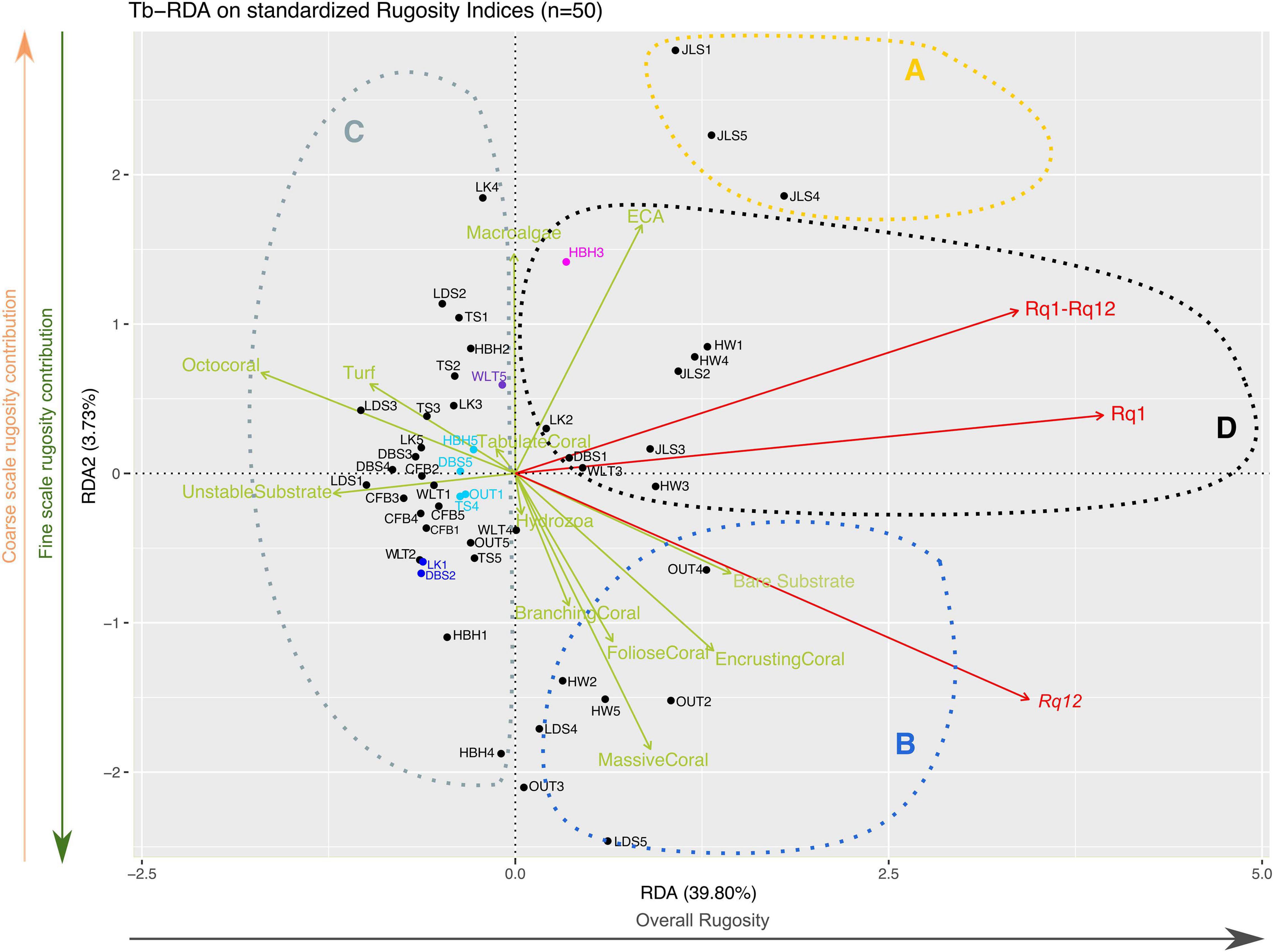
Figure 8. Constrained tb-RDA of transects’ rugosity with their benthic compositions. Red vectors represent the contributions of the rugosity indices to the tb-RDA, while the green vectors represent the benthic categories constraining the tb-RDA. The gray arrow under the x-axis illustrates the overall rugosity gradient between transects, while the green and orange arrows beside the y-axis represent the fine and coarse scale rugosity gradients, respectively. Dashed circles represent the proposed target transect groups used to illustrate potential management strategies in the discussion.
Relationships Between Rugosity Patterns and Benthic Composition
Redundancy analysis (tb-RDA, Figure 8) was performed on standardized rugosity indices constrained by the benthic composition dataset minus the categories that never contributed for more than 5% in any transect. The constrained tb-RDA model containing the 12 remaining benthic categories was significant (ANOVA, F = 2.38, p = 0.007). Values from the variance-inflation factors analysis (vif.cca) ranged from 2.18 (hydrozoa) to 6.54 (encrusting corals). None of the benthic categories had scores over 10, so they were all kept in the final tb-RDA analysis. The adjusted R2 of the global model of the tb-RDA was 25.23%. The first constrained axis (RDA1) explained 39.80% of the total variance explained by the model (3.01), and the second (RDA2) accounted for 3.73%. For comparison purposes, the first two unconstrained axes (PCA1 and PCA2) explained 44.69% and 11.77%, respectively. The RDA1 axis mainly represents the overall rugosity gradient, as Rq1 was 1.39 (Figure 8), Rq12 was 1.22, and Rq1–Rq12 was 1.19. RDA2 mainly represented a decreasing gradient of fine scale rugosity and an increasing gradient of coarse scale rugosity, with a Rq12 of −0.54, Rq1–Rq12 of 0.39, and Rq1 of 0.14 (Figure 8).
Among the constrained variables, four (encrusting, massive, branching, and foliose corals) of the five scleractinian categories had positive scores on the first tb-RDA axis—ranging from 0.47 (encrusting corals) to 0.13 (branching corals)—and negatively on RDA2 (−0.58 to −0.30). Those four categories of corals were more abundant on transects with higher fine scale rugosity contribution (Figure 8). On those same transects, macro-algae cover was also among the lowest observed in our dataset, which is consistent with macro-algae scoring almost perpendicularly to RDA1 (RDA1 = 0.003 and RDA2 = 0.52). The last coral category, tabulate corals, had a negative score on RDA1 but represented a small weight on both RDA1 (−0.04) and RDA2 (0.06). Octocoral had a negative score on RDA1 (−0.60), as did unstable substrate (−0.43) and turf (−0.34). Octocoral, turf, and unstable substrate are characteristic of transects with lower overall rugosities (Figure 8).
Discussion
In this study, we proposed an alternative numerical approach to improve reef rugosity estimations based on high-resolution depth profiles. We recorded depth profiles using the method that Dustan et al. (2013) developed. Dustan’s method made field data collection relatively straightforward and rapid compared to the chain method, photogrammetry, and other 3D modeling field collection methods (Dustan et al., 2013). Yet, our method can be used on any type of depth profile. We adapted the root mean square of the deviation from the assessed surface profile (Rq) with polynomials to estimate different levels of rugosity. Our approach allows researchers to quantify the contributions of coarse and fine rugosity into the overall reef complexity, and allow reef ecologists to estimate rugosity without concern about bathymetric variations throughout the surveyed location, since sea landscape complexity can be estimated as coarse scale rugosity contribution with our method.
Improvements in Rugosity Estimations
Similarly to Wilson et al. (2007) and Young et al. (2017), we found an important observer bias in the qualitative rugosity estimation methods such as the visual rugosity index proposed by Polunin and Roberts (1993). Using visual indices to estimate reef rugosity is neither costly nor time intensive, but this method is subject to observer bias (Young et al., 2017; Bayley et al., 2019). Our study stresses the need to move away from visual estimations of reef rugosity if we want to accurately estimate the role of a reef’s complexity in its resilience capacities and relationship to the benthic and fish communities, and adequately track changes in this parameter over time or geographic ranges.
Chain and rugosity estimations from our theoretical and in situ transects suggested that the chain index poorly accounts for coarse scale rugosity (Table 2). This is a known consequence of the size of the chain link (Knudby and LeDrew, 2007; Friedman et al., 2012)—in our “virtual chain” case, the chain link corresponds to the resolution of the considered transect, which is comprised in our dataset between 12.5 and 19.4 cm. The inaccurate estimations of coarse scale rugosity by the chain method could be detrimental to specific reef organisms, such as large fishes (Wilson et al., 2008; Dustan et al., 2013; Graham and Nash, 2013). We recommend using Rq indices to better estimate reef rugosity and the relationship between rugosity and reef resilience capacity in the face of disturbances.
Importance of Using Multiple Rugosity Indices and Distinguishing Rugosity Types
Using a single rugosity index to estimate reef structural complexity could lead to transects with different rugosity patterns and sources being assigned equal rugosity scores. This is true for the chain index (Knudby and LeDrew, 2007) and the rugosity indices presented in the present study. Indeed, when a single Rq level is considered, transects with different rugosity patterns could yield the same Rq scores for a given polynomial order. Instead of looking at a single Rq level, we recommend looking at three key Rq levels simultaneously: Rq1, which illustrates the overall rugosity of the surveyed profiles; Rq12, which represents the fine scale rugosity of the profiles; and Rq1–Rq12, an estimate of a profile’s coarse scale rugosity.
Multivariate Analyses of Rugosity Indices and Their Potential Uses in Reef Management
Our constrained multivariate analysis highlighted interesting relationships between certain rugosity levels and the main benthic contributors of the transects examined. Indeed, we observed that transects with higher coarse than fine scale rugosity contribution had a larger contribution of macro-algae, but did not necessarily present higher overall rugosity, which is consistent with the expectations in the literature (Chong-Seng et al., 2012), as macro-algae often provide a more flexible structure of the habitat and reduced the fine scale rugosity via space competition between coral and macro-algae (McCook et al., 2001; Chong-Seng et al., 2012). On the other hand, it was surprising that tabulate corals had a negative score on the first RDA axis; this might be caused by our fine scale rugosity size class. Indeed, in our dataset the average interval between two measurements was 15.73 ± 1.50 cm, therefore, our depth profiles might have only recorded the general morphology of the tabulate corals and not its smallest structural variations on their surface (≤ centimeter scale). However, it could also be a consequence of the low abundance of tabulate corals throughout KNP, as highlighted by Ribas-Deulofeu et al. (2021) (average tabulate coral cover in 2015: 2.55 ± 2.01%).
PCA analyses allowed us to visually identify transects with similar patterns of overall, coarse and fine scale rugosity altogether, as they were plotted close together in our multivariate representations (Figures 7, 8), giving us a relative ranking for the transects based on our three major rugosity levels. Eventually, those visualizations could be used to identify clusters of transects or sites that are particularly consequential for specific reef organisms or management strategies (as illustrated for our study case by dashed circles on Figures 7, 8). However, the interpretation of those results and their transcriptions into management strategies will have to be adapted to the studied depth profile resolution and the captured size ranges. For example, with the resolution of our dataset (decimeter to meter), if managers are seeking areas that will be more favorable to larger herbivorous fishes, then they should prioritize transects and sites with higher coarse scale rugosity (Wilson et al., 2008; Dustan et al., 2013), which in our case means the transects in the upper right-hand side of the PCA visualizations—i.e., JLS1, JLS4 or JLS5 (illustrated by the yellow dashed circle A in Figures 7, 8). Alternatively, if managers are seeking to restore or maintain global structural reef complexity, then transects aggregating on the left side of our PCA (illustrated by the gray dashed circle C in Figures 7, 8) could represent high-priority areas for their management strategy, as these transects globally present a low structural complexity at both fine and coarse scales, due to either specific environmental conditions or harmful anthropogenic activities. The lower left-hand sides of our Figures 7, 8 represent transects with higher fine scale rugosity, which are more favorable to small reef-associated organisms such as damselfishes (blue dashed B circle in Figures 7, 8; Wilson et al., 2008; Graham and Nash, 2013; Rogers et al., 2014). Transects in the black dashed D circle have good overall rugosity with good contributions from both coarse and fine scale rugosity, which could be favorable to both larger and smaller reef organisms (Figures 7, 8). In addition, tb-RDA analysis (Figure 8) allows us to identify the functional groups responsible for the key levels of rugosity that managers might seek to improve. Going a step further, linking our Rq indices with the benthic composition of the surveyed transects can allow reef managers to identify the proportion of the overall rugosity they can manage. Indeed, specific management strategies will influence different types of reef organisms and are unlikely to modify the abiotic components of reef rugosity, such as the bathymetric gradient or the geological features of the surveyed locations. Consequently, relative contribution of fine and coarse scale rugosity provided by inhabiting organisms will better inform reef managers of the extent to which they can improve the rugosity of their targeted reefs.
Future Improvements
Our indices allow the distinction of rugosity at a variety of scales. However, size ranges captured by them are constrained by the resolution of the depth profiles, which can be adjusted according to the targeted ecological process. For example, an interest in coral recruitment will probably need a resolution from the millimeter to the decimeter, defining the limits of the fine and coarse rugosities, respectively. In contrast and following the same definition, decimeter to kilometer scales will better respond to the requirements in seascape ecology. In our case, a resolution from the decimeter to the meter better fitted with our focus on benthic community dynamics, which can be translated by the increase/decrease of benthic taxa’s covers and link to our Rq indices via constrained redundancy analysis.
Despite certain similarities between our Rq indices and fractal dimension approaches, such as reflecting rugosity contributions across different scales (Young et al., 2017), the use of polynomial functions in our indices does not allow for a pre-set of size categories for each Rq, but only a post-calculation of the size ranges captured by them. This could constitute the main weakness of our approach and should be the object of further developments to address it. Yet, the strengths of our approach remain in its wide application to various purposes, along with its relative simplicity in both application and computation [in comparison with other approaches (e.g., fractal dimension)].
Conclusion
Overall, our method facilitates the estimation and interpretation of reef rugosity. The joint use of Rq1, Rq12, and Rq1–Rq12 allows researchers to efficiently and quantitatively estimate overall rugosity, fine and coarse scale rugosity, respectively. Estimating both coarse and fine scale rugosities—and not overall reef rugosity alone—is crucial to better understand the relationship between the structural complexity of reefs and their capacity to resist or recover after specific disturbances. Our indices can be used on any depth profiles, from satellite data to fine-scale 3D models, with various resolution scales depending on the researchers’ aims. Our method could also play an important role in reef management by allowing managers to customize their strategies to targeted species or ecosystem functions.
Data Availability Statement
The datasets and python program used for this study can be found as Supplementary Files S1–S3.
Author Contributions
LR-D performed the field investigation, the data analysis, and wrote the initial draft. P-AC and VD helped develop the statistical framework and compute the data. CAC provided financial support and supervised LR-D. All co-authors actively helped LR-D to revise the current manuscript.
Funding
LR-D was the recipient of a fellowship from the Taiwan International Graduate Program, Academia Sinica. P-AC and VD received postdoctoral fellowships from Academia Sinica. VD was the recipient of a grant from the Ministry of Science and Technology of Taiwan (108-2611-M-002-013). This work was funded by the Center for Sustainability Science, Academia Sinica (AS-104-SS-A03) to CAC.
Conflict of Interest
The authors declare that the research was conducted in the absence of any commercial or financial relationships that could be construed as a potential conflict of interest.
Publisher’s Note
All claims expressed in this article are solely those of the authors and do not necessarily represent those of their affiliated organizations, or those of the publisher, the editors and the reviewers. Any product that may be evaluated in this article, or claim that may be made by its manufacturer, is not guaranteed or endorsed by the publisher.
Acknowledgments
We are grateful to Rainer Wunderlich, Derek Soto, and Stephane De Palmas for the fruitful discussion on rugosity. We also thank Éadaoin Close for her help editing the manuscript. Thanks also to Wei-Chieh and Sophie Cheng for their help during the fieldwork, and Aichi Chung for her help with visual estimations of rugosity.
Supplementary Material
The Supplementary Material for this article can be found online at: https://www.frontiersin.org/articles/10.3389/fmars.2021.675853/full#supplementary-material
Supplementary Figure 1 | Theoretical transect profiles with successive polynomial levels fitted.
Supplementary Figure 2 | In situ transect profiles with successive polynomial levels fitted.
Supplementary File 1 | Python program—rugosity calculations.
Supplementary File 2 | Data—depth profiles of the nine theoretical transects.
Supplementary File 3 | Data—depth profiles of the 50 in situ transects.
References
Bayley, D. T. I., Mogg, A. O. M., Koldewey, H., and Purvis, A. (2019). Capturing complexity: field-testing the use of “structure from motion” derived virtual models to replicate standard measures of reef physical structure. PeerJ 7:e6540. doi: 10.7717/peerj.6540
Borcard, D., Gillet, F., and Legendre, P. (2018). Numerical Ecology With R. Cham: Springer. doi: 10.1007/978-3-319-71404-2
Bozec, Y. M., Alvarez-Filip, L., and Mumby, P. J. (2015). The dynamics of architectural complexity on coral reefs under climate change. Glob. Chang. Biol. 21, 223–235. doi: 10.1111/gcb.12698
Burns, J. H. R., Delparte, D., Gates, R. D., and Takabayashi, M. (2015). Utilizing underwater three-dimensional modeling to enhance ecological and biological studies of coral reefs. ISPRS Int. Arch. Photogramm. Remote Sens. Spat. Inf. Sci. XL-5/W5, 61–66. doi: 10.5194/isprsarchives-XL-5-W5-61-2015
Carilli, J. E., Norris, R. D., Black, B. A., Walsh, S. M., and McField, M. (2009). Local stressors reduce coral resilience to bleaching. PLoS One 4:e6324. doi: 10.1371/journal.pone.0006324
Carpenter, K. E., Abrar, M., Aeby, G., Aronson, R. B., Banks, S., Bruckner, A., et al. (2008). One-third of reef-building corals face elevated extinction risk from climate change and local impacts. Science 321, 560–563. doi: 10.1126/science.1159196
Chong-Seng, K. M., Mannering, T. D., Pratchett, M. S., Bellwood, D. R., and Graham, N. A. J. (2012). The influence of coral reef benthic condition on associated fish assemblages. PLoS One 7:e42167. doi: 10.1371/journal.pone.0042167
Darling, E. S., Graham, N. A. J., Januchowski-Hartley, F. A., Nash, K. L., Pratchett, M. S., and Wilson, S. K. (2017). Relationships between structural complexity, coral traits, and reef fish assemblages. Coral Reefs 36, 561–575. doi: 10.1007/s00338-017-1539-z
Darling, E. S., McClanahan, T. R., Maina, J., Gurney, G. G., Graham, N. A. J., Januchowski-Hartley, F., et al. (2019). Social–environmental drivers inform strategic management of coral reefs in the Anthropocene. Nat. Ecol. Evol. 3, 1341–1350. doi: 10.1038/s41559-019-0953-8
Dustan, P., Doherty, O., and Pardede, S. (2013). Digital reef rugosity estimates coral reef habitat complexity. PLoS One 8:e57386. doi: 10.1371/journal.pone.0057386
Ferrari, R., Bryson, M., Bridge, T., Hustache, J., Williams, S. B., Byrne, M., et al. (2016). Quantifying the response of structural complexity and community composition to environmental change in marine communities. Glob. Chang. Biol. 22, 1965–1975. doi: 10.1111/gcb.13197
Figueira, W., Ferrari, R., Weatherby, E., Porter, A., Hawes, S., and Byrne, M. (2015). Accuracy and precision of habitat structural complexity metrics derived from underwater photogrammetry. Remote Sens. 7, 16883–16900. doi: 10.3390/rs71215859
Fofonoff, N. P., and Millard, R. C. (1983). Algorithms for Computation of Fundamental Properties of Seawater. UNESCO. Available online at: https://development.oceanbestpractices.net/handle/11329/109 (accessed October 14, 2019).
Friedman, A., Pizarro, O., Williams, S. B., and Johnson-Roberson, M. (2012). Multi-scale measures of rugosity, slope and aspect from benthic stereo image reconstructions. PLoS One 7:e50440. doi: 10.1371/journal.pone.0050440
González-Rivero, M., Bongaerts, P., Beijbom, O., Pizarro, O., Friedman, A., Rodriguez-Ramirez, A., et al. (2014). The catlin seaview survey kilometre-scale seascape assessment, and monitoring of coral reef ecosystems. Aquat. Conserv. Mar. Freshw. Ecosyst. 24, 184–198. doi: 10.1002/aqc.2505
Graham, N. A. J., and Nash, K. L. (2013). The importance of structural complexity in coral reef ecosystems. Coral Reefs 32, 315–326. doi: 10.1007/s00338-012-0984-y
Graham, N. A. J., Jennings, S., MacNeil, M. A., Mouillot, D., and Wilson, S. K. (2015). Predicting climate-driven regime shifts versus rebound potential in coral reefs. Nature 518, 94–97. doi: 10.1038/nature14140
Harborne, A. R., Mumby, P. J., and Ferrari, R. (2012). The effectiveness of different meso-scale rugosity metrics for predicting intra-habitat variation in coral-reef fish assemblages. Environ. Biol. Fishes 94, 431–442. doi: 10.1007/s10641-011-9956-2
Hoegh-Guldberg, O., Mumby, P. J., Hooten, A. J., Steneck, R. S., Greenfield, P., Gomez, E., et al. (2007). Coral reefs under rapid climate change and ocean acidification. Science 318, 1737–1742. doi: 10.1126/science.1152509
Hoegh-Guldberg, O., Poloczanska, E. S., Skirving, W., and Dove, S. (2017). Coral reef ecosystems under climate change and ocean acidification. Front. Mar. Sci. 4:158. doi: 10.3389/fmars.2017.00158
Hughes, T. P., Baird, A. H., Bellwood, D. R., Card, M., Connolly, S. R., Folke, C., et al. (2003). Climate change, human impacts, and the resilience of coral reefs. Science 301, 929–933. doi: 10.1126/science.1085046
Hughes, T. P., Barnes, M. L., Bellwood, D. R., Cinner, J. E., Cumming, G. S., Jackson, J. B. C., et al. (2017). Coral reefs in the anthropocene. Nature 546, 82–90. doi: 10.1038/nature22901
Hughes, T. P., Bellwood, D. R., Baird, A. H., Brodie, J., Bruno, J. F., and Pandolfi, J. M. (2011). Shifting base-lines, declining coral cover, and the erosion of reef resilience: comment on Sweatman et al. (2011). Coral Reefs 30, 653–660. doi: 10.1007/s00338-011-0787-6
Hughes, T. P., Graham, N. A. J., Jackson, J. B. C., Mumby, P. J., and Steneck, R. S. (2010). Rising to the challenge of sustaining coral reef resilience. Trends Ecol. Evol. 25, 633–642. doi: 10.1016/j.tree.2010.07.011
Kleypas, J. A., Buddemeier, R. W., and Gattuso, J.-P. (2001). The future of coral reefs in an age of global change. Int. J. Earth Sci. 90, 426–437. doi: 10.1007/s005310000125
Knudby, A., and LeDrew, E. (2007). “Measuring structural complexity on coral reefs,” in Proceedings of the American Academy of Underwater Science (AAUS) 26th Symposium, eds N. W. Pollock and J. M. Godfrey, 181–188.
Knudby, A., Pittman, S. J., Maina, J., and Rowlands, G. (2014). “Remote sensing and modeling of coral reef resilience,” in Remote Sensing and Modeling: Advances in Coastal and Marine Resource, eds C. Makowski and C. W. Finkl (Springer), 103–134. doi: 10.1007/978-3-319-06326-3_5
Kohler, K. E., and Gill, S. M. (2006). Coral point count with excel extensions (CPCe): a visual basic program for the determination of coral and substrate coverage using random point count methodology. Comput. Geosci. 32, 1259–1269. doi: 10.1016/J.CAGEO.2005.11.009
Lazarus, M., and Belmaker, J. (2021). A review of seascape complexity indices and their performance in coral and rocky reefs. Methods Ecol. Evol. 12:13557. doi: 10.1111/2041-210x.13557
Legendre, P., and Legendre, L. (2012). Canonical analysis. Dev. Environ. Mod. 24, 625–710. doi: 10.1016/B978-0-444-53868-0.50011-3
Luckhurst, B. E., and Luckhurst, K. (1978). Analysis of the influence of substrate variables on coral reef fish communities. Mar. Biol. 49, 317–323. doi: 10.1007/BF00455026
Magel, J. M. T. T., Burns, J. H. R. R., Gates, R. D., and Baum, J. K. (2019). Effects of bleaching-associated mass coral mortality on reef structural complexity across a gradient of local disturbance. Sci. Rep. 9:2512. doi: 10.1038/s41598-018-37713-1
Maynard, J., Marshall, P., Parker, B., Mcleod, E., Ahmadia, G., van Hooidonk, R., et al. (2017). A Guide to Assessing Coral Reef Resilience for Decision Support. Available online at: www.reefecologic.org (accessed February 24, 2020)
McCook, L., Jompa, J., and Diaz-Pulido, G. (2001). Competition between corals and algae on coral reefs: a review of evidence and mechanisms. Coral Reefs 19, 400–417. doi: 10.1007/s003380000129
McCune, B., and Grace, J. (2002). Analysis of ecological communities. J. Exp. Mari. Biol. Ecol. 289, 91–101. doi: 10.1016/s0022-0981(03)00091-1
Mollica, N. R., Guo, W., Cohen, A. L., Huang, K. F., Foster, G. L., Donald, H. K., et al. (2018). Ocean acidification affects coral growth by reducing skeletal density. Proc. Natl. Acad. Sci. U.S.A. 115, 1754–1759. doi: 10.1073/pnas.1712806115
Pecl, G. T., Araújo, M. B., Bell, J. D., Blanchard, J., Bonebrake, T. C., Chen, I. C., et al. (2017). Biodiversity redistribution under climate change: impacts on ecosystems and human well-being. Science 355:eaai9214. doi: 10.1126/science.aai9214
Pendleton, L. H., Hoegh-Guldberg, O., Langdon, C., and Comte, A. (2016). Multiple stressors and ecological complexity require a new approach to coral reef research. Front. Mar. Sci. 3:36. doi: 10.3389/fmars.2016.00036
Polunin, N. V. C., and Roberts, C. M. (1993). Greater biomass and value of target coral-reef fishes in two small Caribbean marine reserves. Mar. Ecol. Prog. Ser. 100, 167–176. doi: 10.3354/meps100167
Purkis, S. J., Graham, N. A. J., and Riegl, B. M. (2008). Predictability of reef fish diversity and abundance using remote sensing data in Diego Garcia (Chagos Archipelago). Coral Reefs 27, 167–178. doi: 10.1007/s00338-007-0306-y
Ribas-Deulofeu, L., Denis, V., Château, P.-A., and Chen, C. A. (2021). Impacts of heat stress and storm events on the benthic communities of Kenting National Park (Taiwan). PeerJ 9:e11744. doi: 10.7717/peerj.11744
Ribas-Deulofeu, L., Denis, V., De Palmas, S., Kuo, C. Y., Hsieh, H. J., and Chen, C. A. (2016). Structure of benthic communities along the Taiwan latitudinal gradient. PLoS One 11:e0160601. doi: 10.1371/journal.pone.0160601
Richardson, L. E., Graham, N. A. J., Pratchett, M. S., and Hoey, A. S. (2017). Structural complexity mediates functional structure of reef fish assemblages among coral habitats. Environ. Biol. Fishes 100, 193–207. doi: 10.1007/s10641-016-0571-0
Richmond, R. H., Tisthammer, K. H., and Spies, N. P. (2018). The effects of anthropogenic stressors on reproduction and recruitment of corals and reef organisms. Front. Mar. Sci. 5:226. doi: 10.3389/fmars.2018.00226
Risk, M. J. (1972). Fish diversity on a coral reef in the Virgin Islands. Atoll Res. Bull. 153, 1–4. doi: 10.5479/si.00775630.153.1
Rogers, A., Blanchard, J. L., and Mumby, P. J. (2014). Vulnerability of coral reef fisheries to a loss of structural complexity. Curr. Biol. 24, 1000–1005. doi: 10.1016/j.cub.2014.03.026
Syms, C., and Jones, G. P. (2000). Disturbance, habitat structure, and the dynamics of a coral-reef fish community. Ecology 81, 2714–2729.
Vergés, A., Steinberg, P. D., Hay, M. E., Poore, A. G. B., Campbell, A. H., Ballesteros, E., et al. (2014). The tropicalization of temperate marine ecosystems: climate-mediated changes in herbivory and community phase shifts. Proc. R. Soc. B Biol. Sci. 281:20140846. doi: 10.1098/rspb.2014.0846
Wilkinson, C. R. (1999). Global and local threats to coral reef functioning and existence: review and predictions. Mar. Freshw. Res. 50, 867–878. doi: 10.1071/MF99121
Wilson, S. K., Fisher, R., Pratchett, M. S., Graham, N. A. J., Dulvy, N. K., Turner, R. A., et al. (2008). Exploitation and habitat degradation as agents of change within coral reef fish communities. Glob. Chang. Biol. 14, 2796–2809. doi: 10.1111/j.1365-2486.2008.01696.x
Wilson, S. K., Graham, N. A. J., and Polunin, N. V. C. (2007). Appraisal of visual assessments of habitat complexity and benthic composition on coral reefs. Mar. Biol. 151, 1069–1076. doi: 10.1007/s00227-006-0538-3
Yanovski, R., Nelson, P. A., and Abelson, A. (2017). Structural complexity in coral reefs: examination of a novel evaluation tool on different spatial scales. Front. Ecol. Evol. 5:27. doi: 10.3389/fevo.2017.00027
Young, C., Schopmeyer, S., and Lirman, D. (2012). A review of reef restoration and coral propagation using the threatened genus Acropora in the Caribbean and Western Atlantic. Bull. Mar. Sci. 88, 1075–1098. doi: 10.5343/bms.2011.1143
Keywords: structural complexity, rugosity, coral reef, resilience, Taiwan
Citation: Ribas-Deulofeu L, Château P-A, Denis V and Chen CA (2021) Portraying Gradients of Structural Complexity in Coral Reefs Using Fine-Scale Depth Profiles. Front. Mar. Sci. 8:675853. doi: 10.3389/fmars.2021.675853
Received: 04 March 2021; Accepted: 20 July 2021;
Published: 13 August 2021.
Edited by:
Eric Jeremy Hochberg, Bermuda Institute of Ocean Sciences, BermudaReviewed by:
Susana Enríquez, National Autonomous University of Mexico, MexicoDaniel Pech, The South Border College (ECOSUR), Mexico
Copyright © 2021 Ribas-Deulofeu, Château, Denis and Chen. This is an open-access article distributed under the terms of the Creative Commons Attribution License (CC BY). The use, distribution or reproduction in other forums is permitted, provided the original author(s) and the copyright owner(s) are credited and that the original publication in this journal is cited, in accordance with accepted academic practice. No use, distribution or reproduction is permitted which does not comply with these terms.
*Correspondence: Chaolun Allen Chen, Y2FjQGdhdGUuc2luaWNhLmVkdS50dw==
†Present address: Lauriane Ribas-Deulofeu, Institute of Oceanography, National Taiwan University, Taipei, Taiwan