Novel Method for the Estimation of Vertical Temperature Profiles Using a Coastal Acoustic Tomography System

Systems based on remote sensing technology, which use reciprocal acoustic signals to continuously monitor changes in the coastal oceanic environment, are referred to as coastal acoustic tomography (CAT) systems. These systems have been applied in regions in which heavy ship traffics, fishing and marine aquaculture activities make it difficult to establish in situ oceanic sensor moorings. Conventionally, CAT measurements were used to successfully produce horizontal maps of the depth-averaged current velocity and temperature in these coastal regions without attempting to produce a vertical temperature profile. This prompted us to propose a new method for vertical temperature profile estimation (VTPE) from CAT data using the available sea surface temperature (SST), near-bottom temperature (NBT), and water depth. The VTPE method was validated using data-assimilated and tide-included high-resolution ocean model outputs, including tide data, by comparing the estimated and simulated temperatures. Measurements were performed in the southern coastal region of Korea, where two CAT stations were moored to establish a continuous coastal ocean monitoring system. The validation results revealed that the algorithm performed well across all seasons. Sensitivity tests of the VTPE method with reasonable realistic random errors in the SST, NBT, and acoustic travel time measurements demonstrate that the method is applicable to CAT observation data because the monthly mean root-mean-squared difference (RMSD) for the vertical profiles for February, May, August, and November were 0.23, 0.30, 0.50, and 0.24°C, respectively. The VTPE method was applied to the CAT observation datasets acquired in February and August. The transceivers at the CAT stations were at depths 11 and 6 m on average. The RMSD between the estimated and observed temperatures in the middle layer (∼3 m depth) between two stations in February and August were 0.08 and 0.60°C, respectively, the accuracy of which is sufficient in largely time-varying coastal environments. We provide a novel method for continuous coastal subsurface environmental monitoring without interrupting maritime traffic, fishing, and marine aquaculture activities.

Introduction

Sudden temperature changes in coastal marine environments have an unexpected adverse impact on coastal fisheries and the aquaculture industry (Lee et al., 2007; Choi et al., 2009; Kim and Kim, 2010). Recent progress in sea state monitoring systems has enabled us to obtain continuous high-resolution sea surface temperature (SST) fields from satellite remote sensing (Donlon et al., 2012; JPL Our Ocean Project, 2013). However, it is difficult to obtain continuous subsurface temperature measurements without in situ measuring equipment, and it is also challenging to maintain such equipment owing to extensive movements of maritime traffic, the high cost involved, and/or fishing and marine aquaculture activities in coastal seas. Therefore, a remote sensing measurement system that uses acoustic signals and is known as coastal acoustic tomography (CAT) has been suggested (e.g., Kaneko et al., 2020).

The CAT system is an innovative oceanographic technology that can continuously monitor changes in the coastal oceanic environment using reciprocal acoustic signals, regardless of the amount of maritime traffic, and fishing activities. The CAT system was developed on the basis of ocean acoustic tomography, introduced by Munk and Wunsch (1979). Both acoustic tomography systems measure one-way or reciprocally transmitted travel times between sites. In particular, CAT has demonstrated its ability to monitor coastal environmental changes in regions where direct in situ measurements are difficult (Zheng et al., 1997; Park and Kaneko, 2000, 2001; Yamaoka et al., 2002; Taniguchi et al., 2013; Zhu et al., 2013; Zhang et al., 2015; Syamsudin et al., 2017). Acoustic instruments measure sound speed structures in three dimensions between acoustic stations and can produce current and temperature fields. Nevertheless, the outputs of CAT measurements are mainly depth-averaged horizontal temperature and current velocity fields, which are difficult to obtain with traditional estimation methods.

In this study, we introduce a novel method for vertical temperature profile estimation (VTPE) based on the acoustic travel time (ATT) between CAT stations and use additionally available in situ measurements of SST, near-bottom temperature (NBT), and water depth. Using the output of the high-resolution tide-included ocean model, we first validated the performance of the VTPE method using data collected during all four seasons. This entailed comparing the simulated and estimated temperatures for the southern coastal region of Korea, where two CAT experimental points were set up to establish a continuous coastal ocean monitoring system (Figure 1). Then, the VTPE method was applied to the data recorded in situ by the CAT observation system, and the accuracy of the method was verified against independent temperature measurements collected in the middle layer between the CAT stations.

FIGURE 1

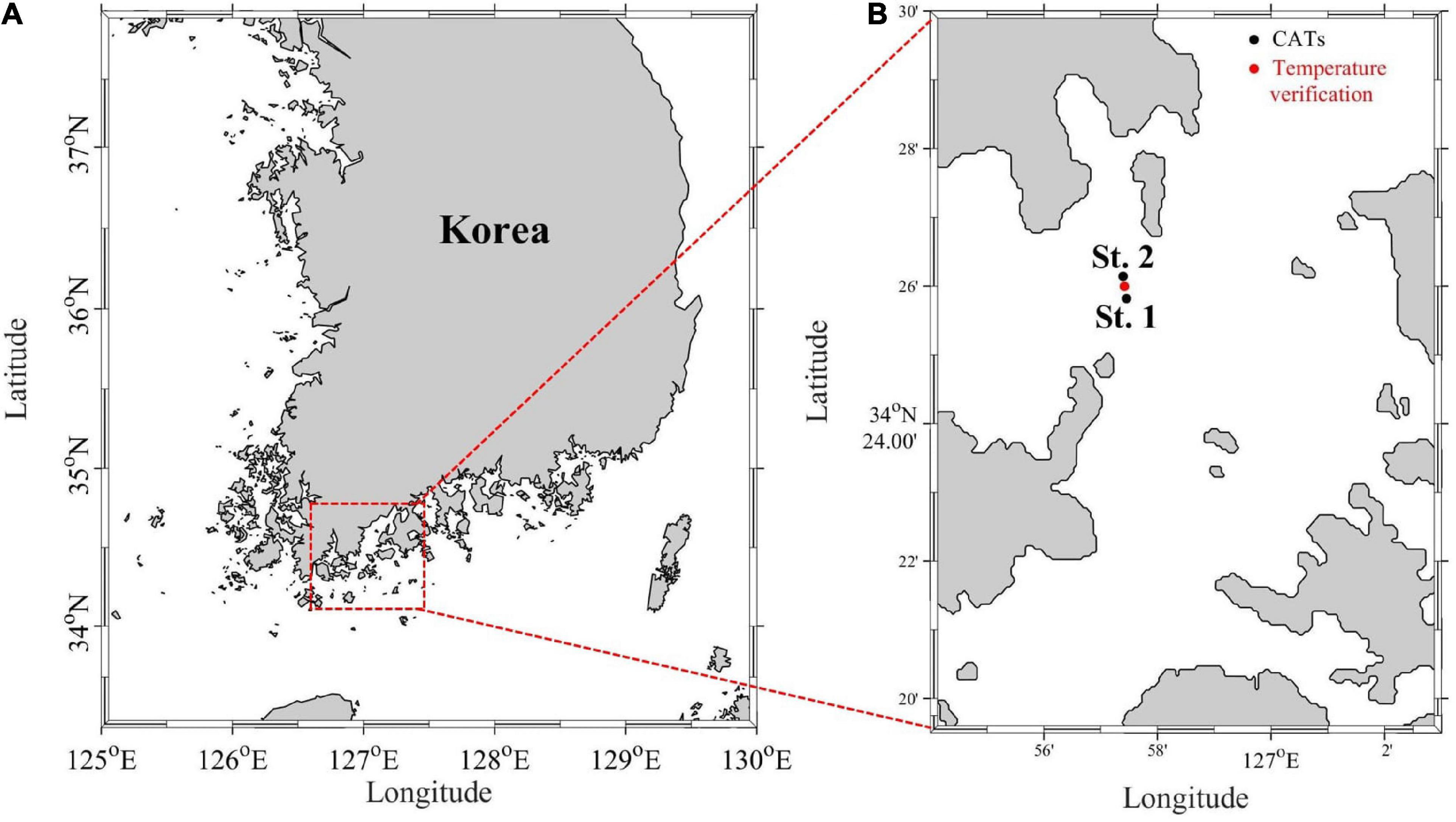
Figure 1. (A) Locations of the two stations used in the CAT field experiment. Station 1 is deeper than Station 2. Temperatures between the estimated and the observed were compared at the location marked by the red dot in (B).

VTPE Procedure

The VTPE method uses the ATT, water depth, SST, and NBT as its inputs. A schematic flowchart of the VTPE method is presented in Figure 2. The method aims to select a plausible vertical temperature profile among the intended vertical temperature profiles based on the fixed water depth, SST, NBT, and measured ATT. The details of the VTPE procedure are as follows.

FIGURE 2

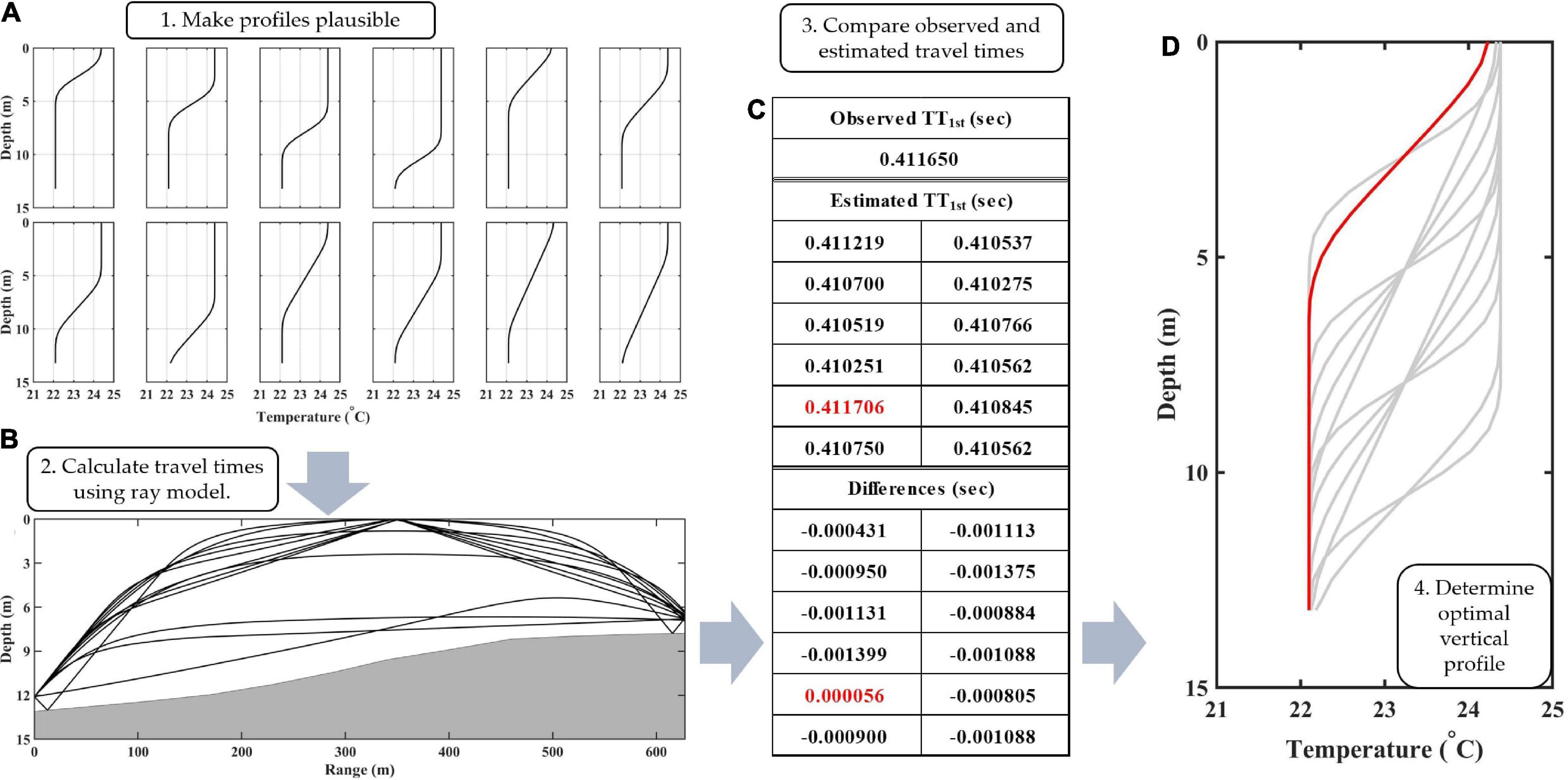
Figure 2. (A) Temperature profiles created using water depth, SST, and NBT. (B) Eigenrays of the ATT_1st in each of the temperature profiles. (C) Example of comparison between observed ATT_1st and calculated ATT_1st. The value of ATT_1st closest to the observed value is displayed in red. (D) The determined optimal profile is plotted as the red line. SST, Sea surface temperature; NBT, Near-bottom temperature; and ATT, Acoustic travel time.

The first step is to create plausible temperature profiles based on the water depth, SST, and NBT. The temperature profiles were set by modifying the thickness and depth of the seasonal thermocline with the fixed water depth, SST, and NBT from the measurements. The thickness and depth of the thermocline were varied in the range of 20, 40, 60, and 80% of the total depth; thus, a pair of SST and NBT values consists of 12 profiles (Figure 2A). The number of profiles is 12 instead of 16 because the thermocline can extend beyond the sea surface or sea bottom when the thickness of thermocline is 60 or 80% and the depth of thermocline is 20 or 80%. Note that all profiles are identical when the SST and NBT are the same.

The second step is to calculate the ATT using each predicted temperature profile. The temperature profiles were converted to sound speed profiles using the equation of Mackenzie (1981) with a fixed salinity of 33 psu, which is the annual mean in the study area. The Bellhop ray-tracing model (Hovem and Dong, 2019), designed to perform two-dimensional acoustic ray-tracing for a given sound speed profile in ocean waveguides with range-dependent bathymetry, is used to estimate the eigenrays associated with ATTs (Figure 2B).

The third step is to determine an optimal temperature profile by comparing the observed ATT with the ATTs calculated using the ray-tracing simulations (Figure 2C). If only the first-arrival acoustic travel time (ATT_1st) is detected in the observation, the algorithm finds the optimal profile with the least difference between the estimated and observed values of ATT_1st (Figure 2D). When the optimal ATT_1st with the least difference is not unique, an optimal vertical profile is produced by averaging the two closest predicted profiles. If both the ATT_1st and second-arrival acoustic travel time (ATT_2nd) are detected during an observation, preferentially, we select the second-arrival acoustic ray among multiple rays in ray-tracing simulations with each plausible profile based on the difference between the measured ATT_1st and ATT_2nd. Then, the optimal temperature profile is determined among profiles when the sum of the differences between the observed and estimated values of ATT_1st and ATT_2nd reaches a minimum.

Validation of VTPE Method

Numerical Ocean Model

The VTPE method was verified by utilizing data from four individual months (February, May, August, and November) in 2016 from data-assimilated three-dimensional fine-resolution numerical ocean model outputs. These outputs were used for the real-time ocean forecast system covering East Asian marginal seas¹. The real-time forecast system has a horizontal resolution of 1/12° in longitude and 1/15° in latitude (Hirose et al., 2013) and is based on the RIAM Ocean Model (RIAMOM), a free-surface primitive general circulation model developed by the Research Institute for Applied Mechanics (RIAM) of Kyushu University (Lee, 1996; Lee et al., 2003). RIAMOM is a three-dimensional z-coordinate model that assumes hydrostatic balance and the Boussinesq approximation. The model uses 40 vertical levels of which the thickness increases with depth, from 1 m at the surface to 880 m near the bottom. The upper six layers are defined at depths of 1, 3, 5, 6.5, 10, 15, and 22 m; thus, the model can represent successive vertical temperature changes in shallow coastal regions. The model includes tides and ocean general circulation and is forced by 6-hourly atmospheric forcings. The gridded SST data (MGDSST) of the Japan Meteorological Agency were used for surface relaxation with a time scale of 3 days. The along-track sea surface height of AVISO was assimilated into the model using a reduced-order Kalman filter. More details about the model configurations appear in the paper by Hirose et al. (2013).

Evaluation of VTPE

The temperature profiles estimated with the use of the VTPE method were compared with those generated by the model for February, May, August, and November to investigate the performance of the method in all four seasons. Figure 3 compares the timeseries of the temperature profiles obtained with the model with those estimated using the VTPE method. For February, the temperature profile was vertically homogeneous. The results obtained with the VTPE method were in good agreement with the output of the model (Figures 3A–C). The monthly mean root-mean-squared difference (RMSD) for the vertical temperature profiles is less than 0.01°C. During May, the seasonal thermocline gradually develops and becomes warmer over time (Figure 3D). The results of the VTPE method were in good agreement with the temperature profiles from the ocean model (Figures 3D,E). The absolute errors in Figure 3F are less than 0.5°C overall, and the monthly mean RMSD for the vertical profiles is approximately 0.05°C. In August, a seasonal thermocline developed, and diurnal and semidiurnal internal fluctuations were evident in early- and mid-August (Figure 3G). These patterns are well reflected in the VTPE-estimated temperature timeseries (Figure 3H). The absolute errors were the largest in August, and most of the errors were distributed in the middle layer, when the seasonal thermocline well developed during the first half of the month (Figure 3I). The monthly mean RMSD for the vertical profiles is 0.18°C. In November, the stratification almost disappeared, similar to February (Figure 3J). The VTPE results corresponded well with the temperature profiles produced as model outputs (Figure 3K). The absolute errors are relatively small; hence, the monthly mean RMSD for the vertical profiles is ∼0.01°C (Figure 3L). The vertical distribution of mean-squared difference (MSD) in the water column at 1-m intervals [(°C)²] was described in histograms on the right of Figures 3C,F,I,L. Overall, the MSD was relatively small at or near the sea surface and sea bottom but increased in the middle layer, particularly when the stratification developed.

FIGURE 3

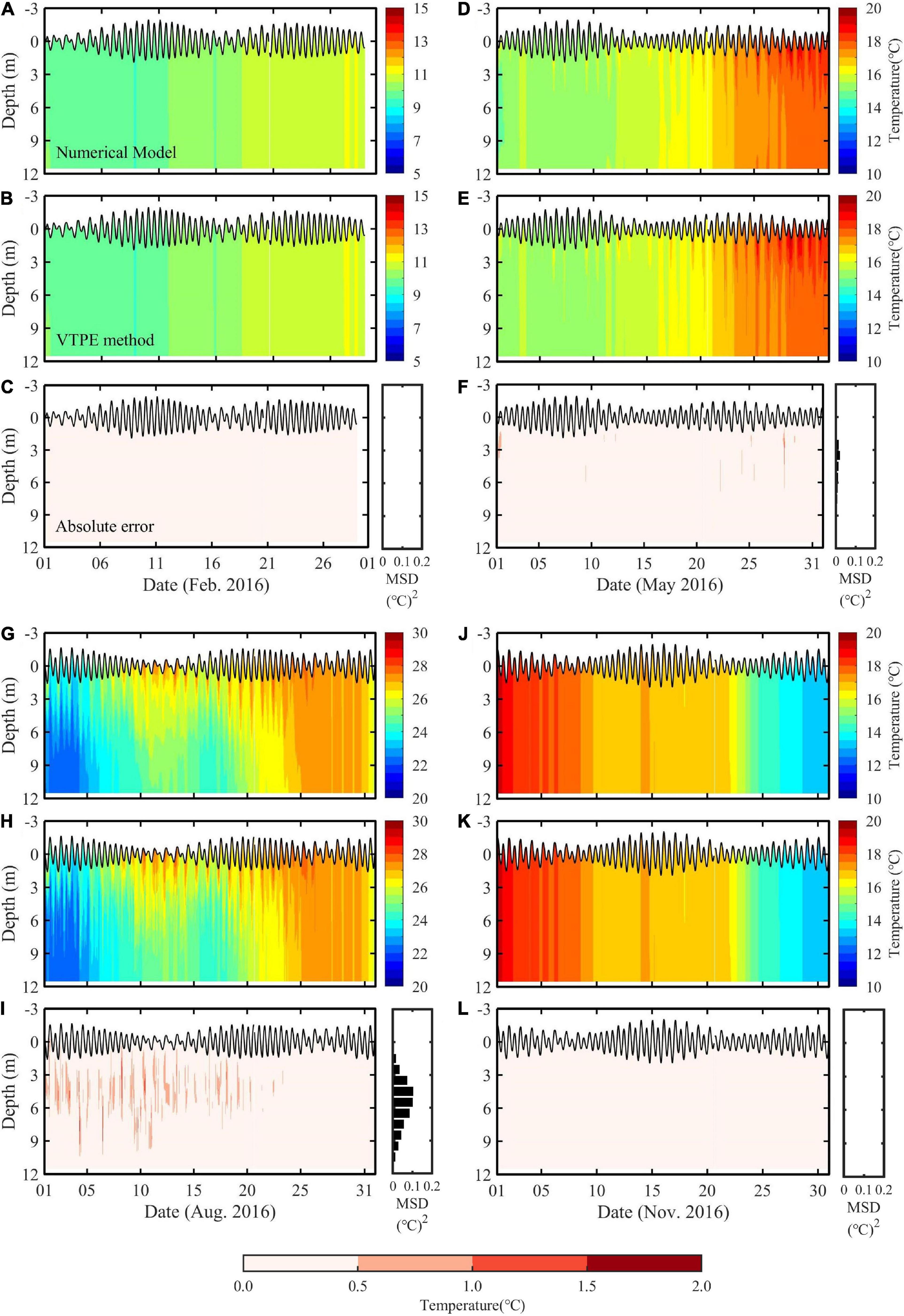
Figure 3. (A,D,G,J) Timeseries of temperature profiles obtained as output of the numerical model for February, May, August, and November 2016 together with the sea level modulations. (B,E,H,K) Timeseries of temperature profile estimated from the VTPE method. (C,F,I,L) Absolute errors in temperature between the output of the numerical model and VTPE results. The colorbar for absolute errors is shown at the bottom. Histograms on the right of (C,F,I,L) represent the vertical distribution of MSD [(°C)²] in the water column at 1-m intervals.

Effects of Tides and Seasonal Thermocline on Ray-Tracing

In general, the tide can significantly impact the sea-level modulations in coastal regions. At our CAT stations, the tidal range had a maximum of ∼4 m, which is sufficiently large compared to the average depth of ∼9 m between the two CAT stations. We conducted ray-tracing simulations using the same temperature profiles (same SST, NBT, and thermocline structure), except for the water depth during the highest and lowest tides, to estimate the influence of tide-induced sea level changes on the propagation of acoustic signals. The 2 months of August and November were selected to investigate the impacts of the tide and seasonal thermocline on the propagation of acoustic signals and ATTs.

Ray-tracing simulations of the propagation of acoustic signals using temperature profiles on August 1, when the difference in SST and NBT was the largest, showed that the acoustic rays differed significantly between the highest and lowest tides in terms of their propagation distance, refraction, and reflection (Figures 4A,B). The simultaneous effects of the tidal elevation and seasonal thermocline complicate the behavior of the acoustic rays, which becomes nonlinear. For example, the first-arrival acoustic rays represented by the red line have different reflection times from the sea surface or sea floor between the highest (three times) and lowest (five times) tides. In November, because the seasonal thermocline almost disappears, only the effect of tidal elevation is predominant (Figures 4C,D); thus, all acoustic rays calculated using temperature profiles recorded on November 23, when the difference between SST and NBT was the smallest, became simpler and more straightforward. The propagation distance of the first-arrival acoustic rays is obviously longer during the highest tides but it is linear. Quantitatively, tidal elevation results in significant differences in ATT_1st with a range of RMSD of 0.53 and 0.12 ms in August and November, respectively, which is sufficiently large to miscalculate the temperature profiles. Hence, the seasonal thermocline and tides in the coastal regions would need to be considered to accurately estimate the temperature profiles from CAT data.

FIGURE 4

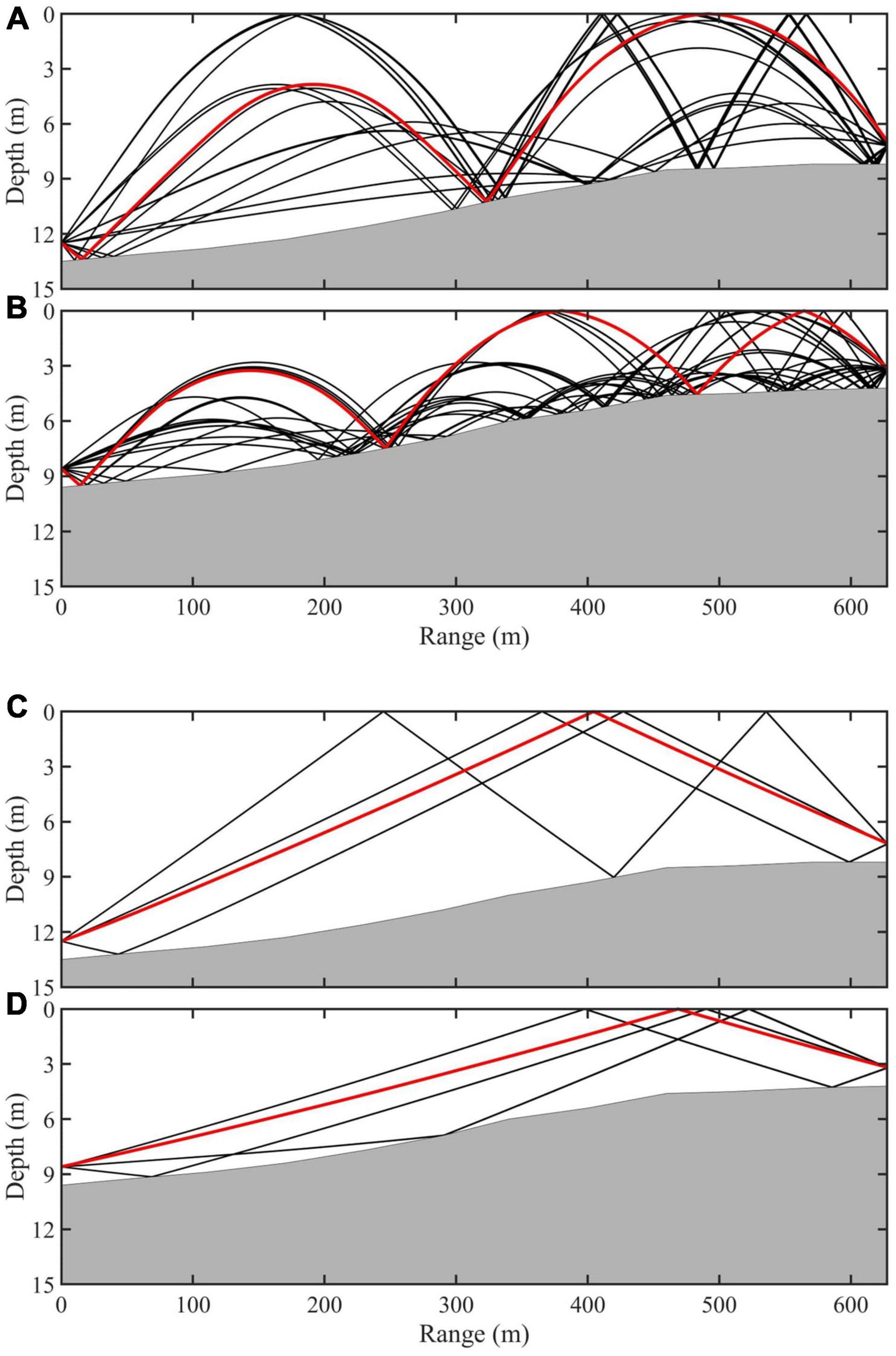
Figure 4. Eigenrays for the (A,C) highest and (B,D) lowest tides in (A,B) August and (C,D) November. The red and black curves indicate the first acoustic ray and those that subsequently arrived, respectively.

Sensitivity Test of VTPE Method

Application of the VTPE method to real ocean measurements could be affected by various measurement errors in SST, NBT, and ATT (first and second ATT measurements in the case of our CAT observation). Sensitivity tests of the VTPE method were carried out by conducting ray-tracing simulations including reasonable observational errors. Four experiments were conducted, one in each of the four seasons: Cases 1 and 2 adopted random errors within ±0.5°C for SST and NBT, respectively. Case 3 added errors of ±0.5% to the ATT, the error of which includes time-varying location of transducers as it is floated in the water, and Case 4 includes all the random errors of Cases 1–3.

The monthly mean RMSD for the vertical profiles was calculated by comparing the temperature that was estimated with the error-included pseudo-observations and those obtained as an output of the numerical model (Table 1). Among the four cases, the RMSDs were similar in Cases 1 and 2 for each of the 4 months: a decrease in the homogenous period (February and November) and an increase in the well-stratified period (May and August). In Case 3, the RMSD differed distinctly between the two periods; the RMSD reached 0.4°C in August, but 0.01°C in February and November. The behavior of the acoustic rays during homogenous months is straightforward compared with that in August and May; hence, ATT errors can have significant impacts on VTPE in well-stratified time.

TABLE 1

Table 1. Sensitivity tests with reasonable random errors in each case.

The results of Case 4 demonstrate an obvious increase in noisy deviation owing to the random errors added (Figure 5). Overall, the differences are smaller at the surface and in layers near the bottom than in the middle layer. For February, the effect of the errors was smaller than in the other months. The estimated temperature profiles appeared noisy but were in good agreement with the model outputs with a monthly mean RMSD for the vertical temperature profiles of 0.23°C. For May, the timeseries of the temperature profiles present more noise than for February, especially after the 25th when the seasonal thermocline developed; hence, the monthly mean RMSD increases to 0.30°C. For August, the absolute errors were the largest among the 4 months with a monthly mean RMSD of 0.50°C. For November, the temperature profiles correspond well with the model outputs with an RMSD of 0.24°C (Table 1).

FIGURE 5

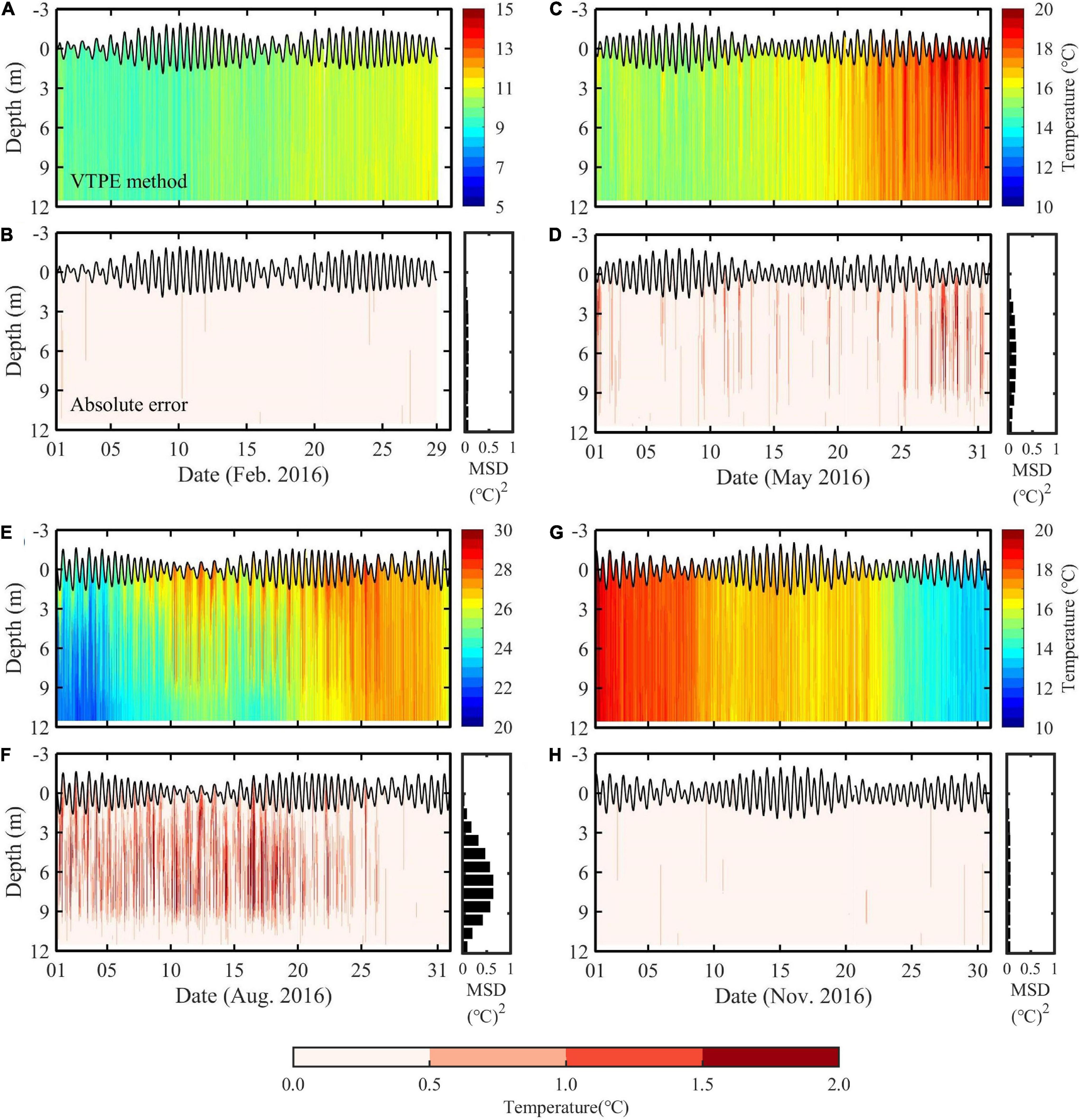
Figure 5. (A,C,E,G) Timeseries of temperature profile estimated with the VTPE method by including the random-error data and (B,D,F,H) absolute errors of the temperature between the output of the numerical model and the VTPE results in (A,B) February, (C,D) May, (E,F) August, and (G,H) November 2016. The colorbar for absolute errors is shown at the bottom. Histograms on the right of (B,D,F,H) represent the vertical distribution of the MSD [(°C)²] in the water column at 1-m intervals.

The vertical distribution of MSD [(°C)²] in the water column at 1-m intervals in case of all random errors included was described in histograms on the right of 5B, 5D, 5F, and 5H. The MSD was relatively small at or near the sea surface and sea bottom but increased in the middle layer, particularly in May and August when the stratification developed.

Application of VTPE Method for in situ Observation

In situ Observations and Distance Correction

For sustainable real-time coastal ocean monitoring, a pilot CAT experiment was carried out near Noryeok Island on the southern coast of Korea in February and August 2019 for 14 and 9 days, respectively (see Figure 1). The transceiver (SonoTube 008/D13) at each of the two stations, separated by ∼630 m, was located ∼1 m above the sea floor, approximate average depths were 11 and 6 m at station 1 and 2, respectively. The transceiver transmitted 10 kHz acoustic signals reciprocally. Their phases were modulated by one period [(2⁸–1) digits] of an eigth-order M-sequence, and the ATT_1st and ATT_2nd were recorded in 1-min intervals. The resolution of ATT measurement is 0.025 ms (=0.000025 s) which is sufficient to differentiate plausible sound-speed and temperature profiles. The pressure at the bottom of the ocean was measured with OMNI instruments (PTM/N/RS485), and temperature sensors (RBRduet³ T.D) were moored at the sea surface, middle layer, and sea floor at three sites: station 1, station 2, and between the two stations (Figure 1B). All data were transmitted instantly to the onshore storage server at the Gwangju Institute of Science and Technology. The VTPE calculations were conducted by using the in situ SST, NBT, and bottom pressure measurements recorded at station 1 (deeper station) and the ATTs. The middle layer (∼3 m depth) temperature was separately measured between stations 1 and 2 to validate the VTPE results.

Temperature estimation using acoustic tomography is very sensitive to the distance between acoustic transceivers (Munk et al., 1995). In our field experiment, the transceiver is moored near the sea floor and connected to a surface barge with a global positioning system (GPS) sensor via a slack mooring cable. Because it was difficult to obtain accurate GPS coordinates of the transceiver from the GPS sensor, we used the following procedure to reduce the distance error. We calculated the mean distance (S), $S=C\overline{\mathrm{\tau }}$, where C is the sound speed computed using NBT, and $\overline{\mathrm{\tau }}$ is the bidirectionally averaged ATT_1st. The distance was then corrected in the acoustic ray-tracing simulations in the second step of the VTPE method.

Application of the VTPE Method to in situ Observations

The temperature profiles for February and August were successfully constructed using the VTPE method. The estimated vertical temperature profile during February 12–26 (with 15 h missing on February 20) is shown in Figure 6. The temperature fluctuates within a range of ±1.5°C from the mean temperature of ∼8°C and represents the typical pattern of a vertically homogeneous temperature change in February. The semidiurnal and diurnal fluctuations in temperature seem to be caused by tidal variability. To verify the VTPE result, the middle-layer temperature was compared to the in situ temperature measured at the site between the two CAT stations (Figure 6B). The timeseries of the in situ measured and the estimated temperatures were in good agreement, and the average RMSD in the middle layer (∼3 m depth) was 0.08°C (Figure 6C).

FIGURE 6

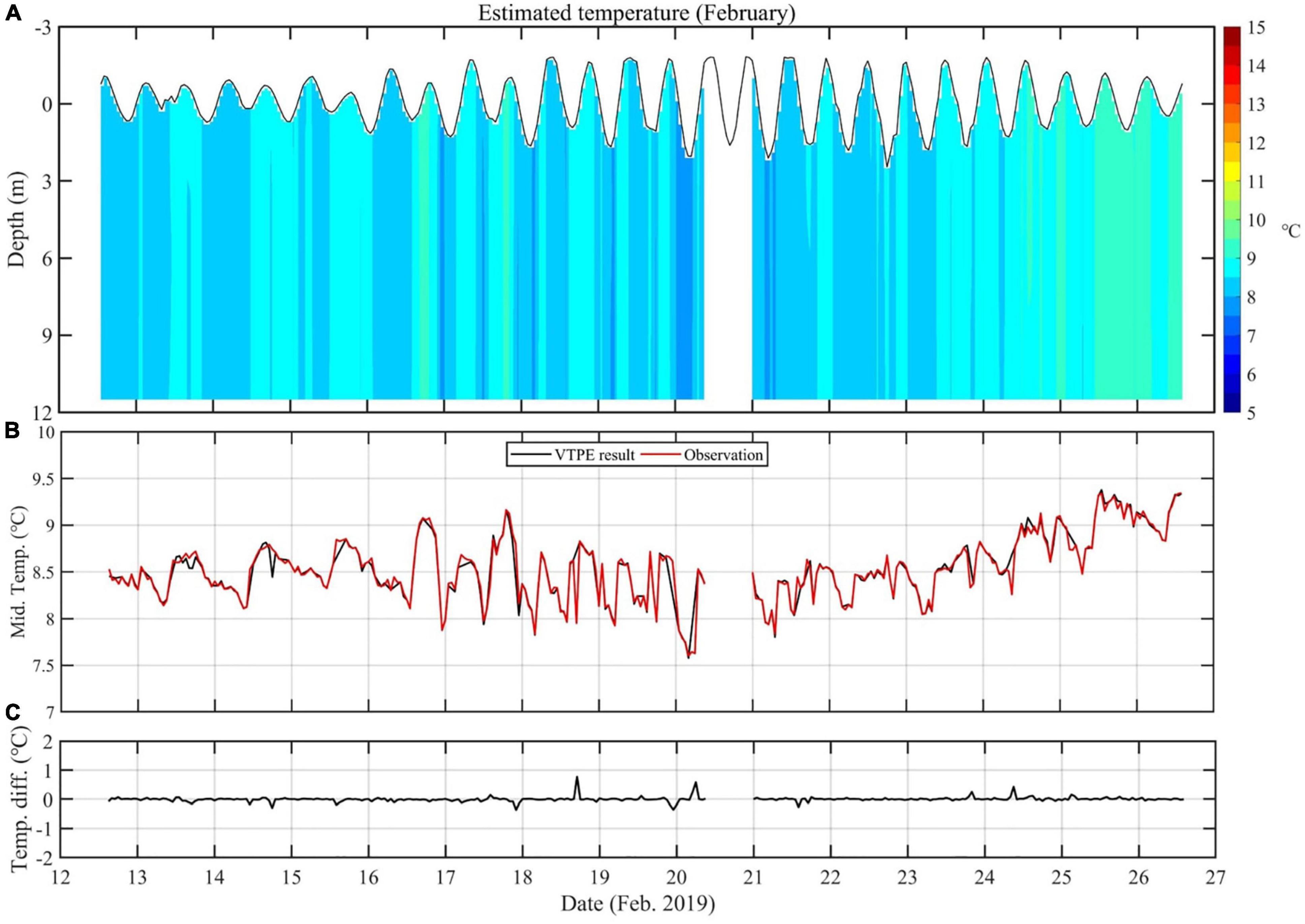
Figure 6. (A) Timeseries of temperature profiles estimated with the VTPE method using the field observation data of February 2019. Note that the SST observation failed for 15 h on February 20. (B) Comparison of the middle-layer temperatures that were estimated and measured in situ at the site between the two CAT stations. (C) Difference between the two timeseries of temperatures shown in (B).

The timeseries of the estimated vertical temperature profile for the period August 1–9 is shown in Figure 7A. The temperature profile describes a stratified water column, a typical structure that is observed in August, and the development of a seasonal thermocline on August 8–9. The overall temporal variability in the temperature seems to be associated with semidiurnal and diurnal tides, although surface tides of semidiurnal frequency are weak. The estimated middle-layer temperature was compared with that measured in situ at the site between the two CAT stations (Figure 7B). The temperature estimated using the VTPE method is in good correspondence with that measured in situ, including the increasing tendency on August 7–9. The average RMSD between the estimated and measured temperatures in the middle layer is 0.60°C, which is satisfactory considering the highly fluctuating conditions in coastal regions (Figure 7C).

FIGURE 7

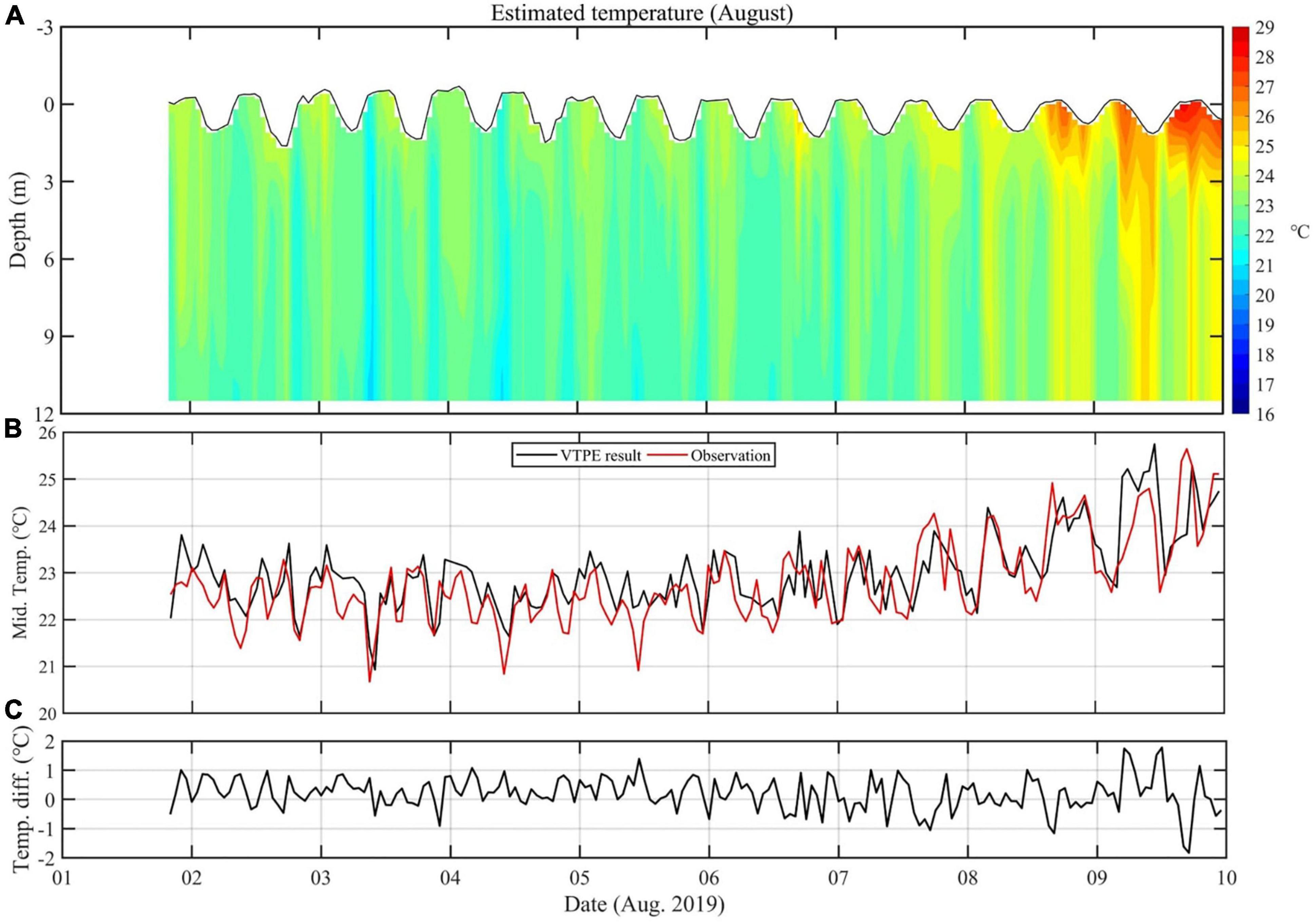
Figure 7. (A) Timeseries of temperature profiles estimated from the VTPE method using the field observation data gathered in August 2019. (B) Comparison of middle-layer temperatures between the estimated and the in situ measurement at a site between the two CAT stations. (C) Difference of the two timeseries of temperatures shown in (B).

In addition, we compared the performance of the VTPE method with existing widely used regularized inverse method (Zhu et al., 2013; Zhang et al., 2015; Syamsudin et al., 2017) with and without the distance correction, though the inverse method has not been used to produce vertical temperature profile in previous studies. The middle-layer temperature RMSD of 6.21, 0.96, and 0.60°C was obtained from the inverse method without and with the distance correction, and from the VTPE method with the distance correction, respectively (see Supplementary Material), indicating that the VTPE method and the distance correction suggested here should be valid and practical for the CAT data obtained from non-fixed transceivers.

Summary and Conclusion

We propose a novel method for VTPE from CAT systems using additional available data, such as SST, NBT, and water depth. The proposed VTPE method is validated using data-assimilated and tide-included high-resolution ocean model outputs by comparing the estimated and model-simulated temperatures in the southern coastal region of Korea, where the CAT stations have been moored to establish a continuous coastal ocean monitoring system. Our novel VTPE method was then applied to the in situ observation data.

The validation of the VTPE method using the numerical ocean model outputs reveals that the algorithm delivers good performance for all seasons, with monthly mean RMSD for the vertical profiles of 0.01, 0.05, 0.18, and 0.01°C in February, May, August, and November, respectively. Sensitivity tests with reasonable random errors added to SST, NBT, and ATT demonstrate that the method can reproduce accurate temperature profiles with somewhat increased monthly mean RMSD for the vertical profiles of 0.23, 0.30, 0.50, and 0.24°C in February, May, August, and November, respectively. The VTPE method was applied to in situ observation data for 15 days in February and 9 days in August. The VTPE results realistically reproduce the seasonality and high-frequency variabilities of temperature. Comparisons of middle-layer temperature between the VTPE-estimated and the observed temperature in February and August revealed mean RMSDs of 0.08 and 0.60°C, respectively, which is satisfactory for coastal ocean monitoring.

Although the data from the two CAT stations enabled the estimation of a one-dimensional temperature profile, the VTPE method proposed in this study can pave the way for continuous monitoring of two- and three-dimensional temperature fields by combining multiple CAT stations. The VTPE method, monitoring subsurface temperature profile, will help crisis managements in coastal fisheries and the aquaculture industries due to impacts of warming climate and marine heat wave (Caputi et al., 2016; Rogers et al., 2021).

The estimated temperature profile using two CAT stations produces spatially averaged range-independent temperature profiles between two stations. Estimation of the range-dependent vertical profiles considering spatial scales of oceanic phenomena would be important for high-resolution coastal monitoring. Also, the effect of salinity on the VTPE method was not considered in this study; however, it could have an impact on ATTs when events such as fresh water discharge or intrusion and heavy precipitation occur. Lastly, the VTPE method might have a limitation in regions where the stratification is very complicated due to such as significant temperature inversion. Therefore, these problems would need to be addressed in future to improve the VTPE method.

Data Availability Statement

The raw data supporting the conclusions of this article will be made available by the authors, without undue reservation.

Author Contributions

YP: primary writing and calculation. CJ: writing and discussion. HS, YC, J-YC, and E-JL: data collection and discussion. JSK: in situ observation and data management. J-HP: overall coordination and discussion. All authors modify the manuscript.

Funding

This research was supported by the “Development of Ocean Acoustic Echo Sounders and Hydro-Physical Properties Monitoring System” project and “Development of 3-D Ocean Current Observation Technology for Efficient Response to Maritime Distress” project (20210642), funded by the Ministry of Ocean and Fisheries, South Korea.

Conflict of Interest

YP and YC were employed by the companies Underwater Survey Technology 21 and the Geosystem Research Corporation, respectively.

The remaining authors declare that the research was conducted in the absence of any commercial or financial relationships that could be construed as a potential conflict of interest.

Publisher’s Note

All claims expressed in this article are solely those of the authors and do not necessarily represent those of their affiliated organizations, or those of the publisher, the editors and the reviewers. Any product that may be evaluated in this article, or claim that may be made by its manufacturer, is not guaranteed or endorsed by the publisher.

Supplementary Material

The Supplementary Material for this article can be found online at: https://www.frontiersin.org/articles/10.3389/fmars.2021.675456/full#supplementary-material

Footnotes

1. ^ http://dreams-c1.riam.kyushu-u.ac.jp/vwp/

References

Caputi, N., Kangas, M., Denham, A., Feng, M., Pearce, A., Hetzel, Y., et al. (2016). Management adaptation of invertebrate fisheries to an extreme marine heat wave event at a global warming hot spot. Ecol. Evol. 6, 3583–3593. doi: 10.1002/ece3.2137

PubMed Abstract | CrossRef Full Text | Google Scholar

Choi, H.-S., Myoung, J.-I., Park, M.-A., and Cho, M.-Y. (2009). A study on the summer mortality of Korean rockfish Sebastes schlegeli in Korea. J. Fish Pathol. 22, 155–162.

Google Scholar

Donlon, C. J., Martin, M., Stark, J., Roberts-Jones, J., Fiedler, E., and Wimmer, W. (2012). The operational sea surface temperature and sea ice analysis (OSTIA) system. Remote Sens. Environ. 116, 140–158. doi: 10.1016/j.rse.2010.10.017

CrossRef Full Text | Google Scholar

Hirose, N., Takayama, K., Moon, J.-H., Watanabe, T., and Nishida, Y. (2013). Regional data assimilation system extended to the East Asian marginal seas. Sea Sky 89, 43–51.

Google Scholar

Hovem, J. M., and Dong, H. (2019). Understanding ocean acoustics by eigenray analysis. J. Mar. Sci. Eng. 7:118. doi: 10.3390/jmse7040118

CrossRef Full Text | Google Scholar

JPL Our Ocean Project (2013). GHRSST Level 4 G1SST Global Foundation Sea Surface Temperature Analysis. Pasadena, CA: PO.DAAC. doi: 10.5067/GHG1S-4FP01

CrossRef Full Text | Google Scholar

Kaneko, A., Zhu, X.-H., and Lin, J. (2020). Coastal Acoustic Tomography. Amsterdam: Elsevier, 347.

Google Scholar

Kim, S.-H., and Kim, D.-S. (2010). Effect of temperature on catches of anchovy and sea mustard (Undaria pinnatifida) in southern part of east sea of Korea. J. Korean Soc. Mar. Environ. Saf. 16, 153–159.

Google Scholar

Lee, H. C. (1996). A Numerical Simulation for the Water Masses and Circulations of the Yellow Sea and the East China Sea, Ph.D. thesis. Fukuoka: Kyushu University.

Google Scholar

Lee, H.-J., Yoon, J.-H., Kawamura, H., and Kang, H.-W. (2003). Comparison of RIAMOM and MOM in modeling the East Sea/Japan Sea circulation. Ocean Polar Res. 25, 287–302. doi: 10.4217/OPR.2003.25.3.287

CrossRef Full Text | Google Scholar

Lee, Y.-H., Shim, J.-M., Kim, Y.-S., Hwang, J.-D., Yoon, S.-H., Lee, C., et al. (2007). The variation of water temperature and the mass mortalities of sea squirt, Halocynthia roretzi along Gyeongbuk coasts of the east sea in summer, 2006. J. Korean Soc. Mar. Environ. Saf. 13, 15–19.

Google Scholar

Mackenzie, K. V. (1981). Nine-term equation for sound speed in the oceans. J. Acoust. Soc. Am. 70, 807–812. doi: 10.1121/1.386920

CrossRef Full Text | Google Scholar

Munk, W., Worcester, P., and Wunsch, C. (1995). Ocean Acoustic Tomography. Cambridge, MA: Cambridge University Press, 212.

Google Scholar

Munk, W., and Wunsch, C. (1979). Ocean acoustic tomography: a scheme for large scale monitoring. Deep Sea Res. A Oceanogr. Res. Pap. 26, 123–161. doi: 10.1016/0198-0149(79)90073-6

CrossRef Full Text | Google Scholar

Park, J.-H., and Kaneko, A. (2000). Assimilation of coastal acoustic tomography data into a barotropic ocean model. Geophys. Res. Lett. 27, 3373–3376.

Google Scholar

Park, J.-H., and Kaneko, A. (2001). Computer simulation of coastal acoustic tomography by a two-dimensional vortex model. J. Oceanogr. 57, 593–602.

Google Scholar

Rogers, L. A., Wilson, M. T., Duffy-Anderson, J. T., Kimmel, D. G., and Lamb, J. F. (2021). Pollock and “the Blob”: impacts of a marine heatwave on walleye pollock early life stages. Fish. Oceanogr. 30, 142–158. doi: 10.1111/fog.12508

CrossRef Full Text | Google Scholar

Syamsudin, F., Chen, M., Kaneko, A., Adityawarman, Y., Zheng, H., Mutsuda, H., et al. (2017). Profiling measurement of internal tides in Bali Strait by reciprocal sound transmission. Acoust. Sci. Technol. 38, 246–253. doi: 10.1250/ast.38.246

CrossRef Full Text | Google Scholar

Taniguchi, N., Huang, C.-F., Kaneko, A., Liu, C.-T., Howe, B. M., Wang, Y.-H., et al. (2013). Measuring the Kuroshio current with ocean acoustic tomography. J. Acoust. Soc. Am. 134, 3272–3281. doi: 10.1121/1.4818842

CrossRef Full Text | Google Scholar

Yamaoka, H., Kaneko, A., Park, J.-H., Zheng, H., Gohda, N., Takano, T., et al. (2002). Coastal acoustic tomography system and its field application. IEEE J. Ocean. Eng. 27, 283–295.

Google Scholar

Zhang, C., Kaneko, A., Zhu, X., and Gohda, N. (2015). Tomographic mapping of a coastal upwelling and the associated diurnal internal tides in Hiroshima Bay, Japan. J. Geophys. Res. Oceans 120, 4288–4305. doi: 10.1002/2014JC010676

CrossRef Full Text | Google Scholar

Zheng, H., Gohda, N., Noguchi, H., Ito, T., Yamaoka, H., Tamura, T., et al. (1997). Reciprocal sound transmission experiment for current measurement in the Seto Inland Sea, Japan. J. Oceanogr. 53, 117–127.

Google Scholar

Zhu, X.-H., Kaneko, A., Wu, Q., Zhang, C., Taniguchi, N., and Gohda, N. (2013). Mapping tidal current structures in Zhitouyang Bay, China, using coastal acoustic tomography. IEEE J. Ocean. Eng. 38, 285–296. doi: 10.1109/JOE.2012.2223911

CrossRef Full Text | Google Scholar