Impact of Thermohaline Conditions on Vertical Variability of Optical Properties in the Gulf of Finland (Baltic Sea): Implications for Water Quality Remote Sensing

Vertical variability of inherent optical properties (IOPs) affect the water quality retrievals from remote sensing data. Here, we studied the vertical variability of IOPs and simulated apparent optical properties (AOPs) in the Gulf of Finland (Baltic Sea) under three characteristic (non)stratification conditions. In the case of mixed water column, the vertical variability of optically significant constituents (OSC) and IOPs was relatively small. While in case of stratified water column the IOPs of surface layer were three times higher compared to the IOPs below the thermocline and the IOPs were strongly correlated with the physical parameters (temperature, salinity). Measurements of IOPs in stratified water column showed that the ratio of scattering (b(440)) to absorption (a(440)) changed under the thermocline (b(440)/a(440) < 1) i.e., absorption became the dominant component of attenuation under thermocline while the opposite is true for the upper layer. Simulated (from IOPs) spectral irradiance reflectance (R(λ)) and spectral diffuse attenuation coefficient (K_d(λ)) from deeper layers (below thermocline) have significantly smaller magnitude and smoother shape. This becomes relevant during upwelling events—a common process in the coastal Baltic Sea. We quantified the effect of upwelling on surface water properties using simulated AOPs. The simulated AOPs (from IOPs measurements) showed a decrease of the signal up to 68.8% and an increase of optical depth (z₉₀(λ)) from 2.3 to 4.3 m in the green part of the spectrum in case upwelled water mass reaches the surface. In the coastal waters a vertical decrease of K_d(λ) in the PAR region (400–700 nm) by 6.8% (surface to 20 m depth) was observed, while vertical decrease of chlorophyll-a (Chl-a) and total suspended matter (TSM) was 31.7 and 42.1%, respectively. The ratio R(490)/R(560)≥0.77 indicates also the upwelled water mass. The study showed that upwelling is a process that, in addition to biological activity, horizontal transport of OSC, and temperature changes, alters the optical signal of surface water measured by a remote sensor. Knowledge about the vertical variability of IOPs and AOPs relation to upwelling can help the parametrisation of remote sensing algorithms for retrieving water quality estimates in the coastal regions.

Introduction

The remote sensing of ocean colour is a valuable tool for synoptic regional- and global-scale water-quality data estimation [e.g., the concentration of chlorophyll-a (Chl-a) and total suspended matter (TSM)]. Continuous monitoring of the optical quality of water bodies helps to understand different natural processes better, as well as to detect environmental threats such as eutrophication and harmful algal blooms (Ritchie et al., 2003; Glasgow et al., 2004). However, the interpretation of data from passive optical remote sensing is sometimes complicated, not only because of the disturbing influence of the atmospheric effects but also because of some specific characteristics of the object under investigation—the upper layer of the ocean. This is particularly true in the case of marginal seas and inland waters. These waters are optically complex and commonly known as Case 2 waters (Morel and Prieur, 1977), being a function of at least three optically significant constituents (OSC) [phytoplankton pigments, coloured dissolved organic matter (CDOM), and total suspended matter], which may vary independently of one another.

In the Baltic Sea, the composition and concentrations of OSC are highly variable over short spatial scales. Hence, standard remote sensing algorithms developed for Case 2 waters often fail inthis area (e.g., Attila et al., 2013, 2018; Toming et al., 2017). In open and coastal waters of the Baltic Sea, CDOM is the dominant optical component (Kirk, 1984; Kowalczuk et al., 2006; Kratzer and Tett, 2009; Kratzer and Moore, 2018). For instance, according to Kratzer and Moore (2018), the CDOM absorption values range between 0.6 and 1.2 m^–1 (Gulf of Finland), 1.5 and 13.0 m^–1 (Gulf of Riga), and 0.2 and 0.3 m^–1 (Bornholm Sea). In the coastal areas, there are also significant loads of TSM, which increase with proximity to the coast (Kratzer and Tett, 2009). Additionally, Kyryliuk and Kratzer (2019) showed that the Gulf of Gdańsk and Gulf of Riga, which are shallow coastal basins of the Baltic Sea, have a large variability of TSM concentrations, compared to the other basins. The mean values (±standard deviation) over a 3-year period (summer) were 2.80 ± 3.90 g m^–3 and 1.56 ± 2.00 g m^–3, respectively. In addition to spatial variability OSC also show great seasonal variation in the Baltic Sea. The phytoplankton distribution is strongly influenced by the temperature of surface water and the availability of specific nutrients (nitrate, phosphate). Diatoms and dinoflagellates dominate the spring bloom occurring after ice melt and cyanobacteria dominate during summer and early autumn (Wasmund, 1994; Gasinaite et al., 2005; Kownacka et al., 2018; Hjerne et al., 2019). In this case, the optical properties of these phytoplankton groups are so different that some studies have indicated that seasonal remote sensing algorithms are needed (Ligi et al., 2017; Simis et al., 2017). According to the review by Kratzer and Moore (2018) the Chl-a variability in the Baltic Sea ranges from 0.3 to 130 mg m^–3 (in the Gulf of Finland from 1.2 to 130 mg m^–3). From the high-resolution Hyperion imagery, Reinart and Kutser (2006) showed that the chlorophyll concentration may rise up to ∼300 mg m^–3 during cyanobacteria bloom in the Gulf of Finland. Kutser (2004) showed concentrations up to 1,000 mg m^–3 in case of thick cyanobacterial accumulations.

In addition, the coastal zones of the Baltic Sea are often affected by upwellings induced by alongshore winds. This causes the mixing of clear water masses from deeper layers and turbid surface layer water (Gidhagen, 1987; Myrberg and Andrejev, 2003; Lehmann et al., 2012; Omstedt et al., 2014). Numerous studies of this phenomenon in the Baltic Sea have been carried out using remote sensing methods (Kahru et al., 1995; Lehmann et al., 2012; Omstedt et al., 2014), model simulations (Myrberg and Andrejev, 2003; Zhurbas et al., 2008; Laanemets et al., 2009; Väli et al., 2011) and field observations (Haapala and Alenius, 1994; Vahtera et al., 2005; Suursaar and Aps, 2007; Kuvaldina et al., 2010; Kikas and Lips, 2016). The narrow, elongated Gulf of Finland, an easternmost sub-basin of the Baltic Sea, is a well-known region of upwellings during the summer and autumn months when the water masses are relatively strongly stratified (Zhurbas et al., 2008; Gurova et al., 2013; Kikas and Lips, 2016). In this gulf, upwelling along one coast is usually accompanied by downwelling along the opposite coast (e.g., Zhurbas et al., 2008; Lips et al., 2009). Upwelling near the northern coast of the Gulf of Finland is induced by south-westerly winds and along the southern coast by north-easterly winds. Even though upwelling in the southern nearshore is less frequent (about 25% of the time) and not as persistent as near the northern coast (about 30% of the time) (Myrberg and Andrejev, 2003), intensive upwellings also occur near the southern coast of the gulf (Lips et al., 2009; Uiboupin and Laanemets, 2009). The changing wind patterns have apparently increased their frequency in the recent past (Soomere et al., 2015). In addition to changes in the temperature and salinity fields, upwelling events also affect the transport and distribution of sediments and dissolved substances in the marine environment (Nowacki et al., 2009; Dabuleviciene et al., 2018), thus affecting the inherent optical properties (IOPs) of the surface water. Moreover, upwelling plays a crucial role in boosting biological productivity as nutrient-rich water is advected upward into the photic layer, where the process of photosynthesis is promoted (Vahtera et al., 2005; Laanemets et al., 2009; Lips et al., 2009; Uiboupin et al., 2012). Usually the chlorophyll concentrations increase several days after the start of upwelling event. In the early phase (“active phase”) of the upwelling the advected water has low temperature and low OSC concentrations which will increase if the upwelled water remains in the euphotic zone.

Variation of IOPs is an indicator of changes in the concentrations and types of OSC in water. In particular, the light absorption coefficient (a(λ)) and backscattering coefficient (b_b(λ)) are important for optical modelling, since the reflectance can be derived from a function of the ratio of these coefficients. Additionally, these parameters play a key role in governing light propagation in the water column (Gordon, 1988; Morel and Gentili, 1993). Therefore, it is important to understand horizontal and vertical variations of the IOPs in different water masses in order to obtain reasonable estimates of water quality parameters from remote sensing imagery for the optically complex water bodies.

The objectives of the current study are: (1) to improve the knowledge about the vertical variability of IOPs in the coastal zone of Gulf of Finland (Baltic Sea); (2) to characterise the effect of different hydrodynamic conditions on vertical variability of IOPs; (3) and to quantify the impact of upwelling events on the signal measured by the optical remote sensor (using simulated reflectance).

Materials and Methods

The Study Area

The Gulf of Finland is a eutrophied elongated basin in the north-eastern part of the Baltic Sea (Figure 1). It is relatively shallow, with a mean depth of 37 m and a maximum depth of 123 m (Paldiski Deep). The total water volume is about 1098 km³ (Leppäranta and Myrberg, 2009). Topographically, the Gulf is a direct continuation of the Baltic Proper and becomes shallower toward its eastern end. The surface area (29,948 km²) is small compared with the catchment area (423,000 km²) (HELCOM, 2015). The water column in deeper areas is also vertically stratified. A seasonal thermocline usually forms at the beginning of May and starts to erode by the end of August. The thermocline is usually situated at a depth of 10–20 m in such a way that a three-layer vertical structure can be distinguished: the upper mixed layer, the cold intermediate layer, and the near-bottom layer (Alenius et al., 1998; Liblik and Lips, 2011). During the winter, the water column is mixed down to the depth of the permanent halocline at 60–80 m (Haapala and Alenius, 1994; Alenius et al., 1998). The Gulf is strongly influenced by river runoff (114 km³/year), primarily from the Neva, and this influence is apparent not only in the low salinity but also in the optical properties of these waters (Alenius et al., 2003; Vazyulya et al., 2014; Ylöstalo et al., 2016; Sipelgas et al., 2018). The algal growth season is generally from early May to late August (Jaanus et al., 2011). Therefore, factors causing increased light attenuation (e.g., organic and inorganic matter) vary both spatially and temporally in the study area.

FIGURE 1

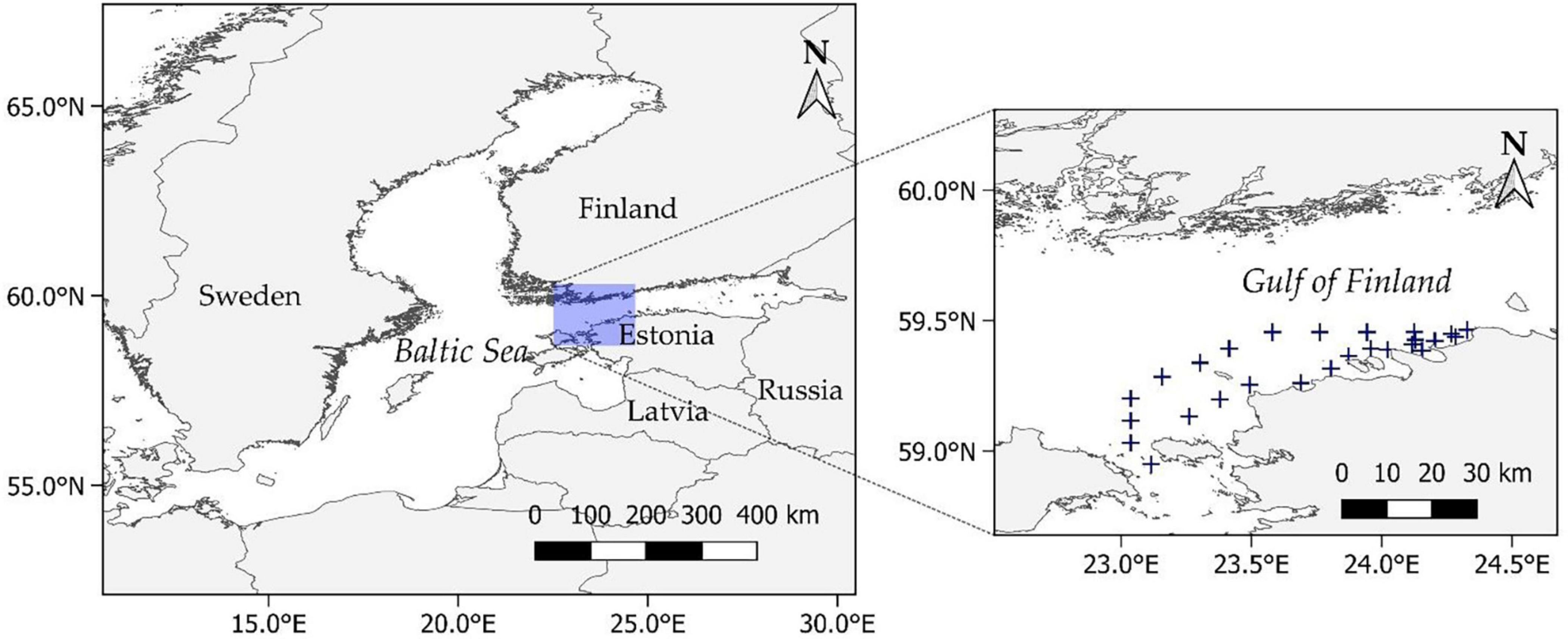
Figure 1. Study area and location of sampling stations.

In situ Data

The in situ measurements for this study were conducted during seven field campaigns (Table 1). The IOPs measurements were performed during the two summers of 2015 (on July 20, July 30–31, August 12, August 25) and 2016 (on July 26–27 and August 3–4), and reflectance measurements to compare the results obtained from previous campaigns were performed during one campaign in the summer of 2018. Additionally, water samples from three different depths (surface layer (0–m), 10 m depth, and 20 m depth) were collected with a rosette sampler, and Secchi depth measurements were performed with a standard white disc with a 30 cm diameter. Figure 1 shows the locations of in situ measurement stations.

TABLE 1

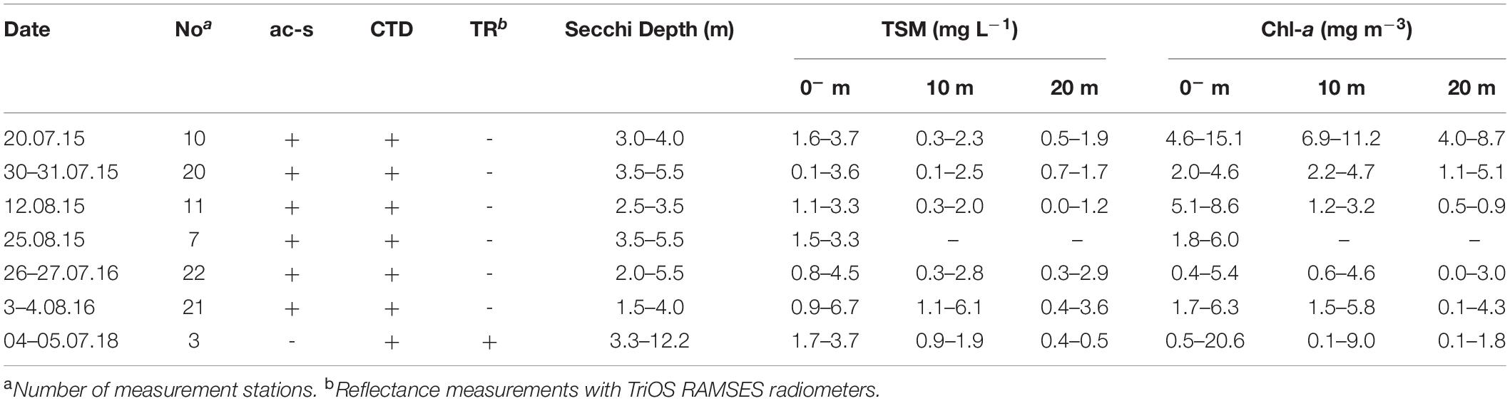
Table 1. A summary of in situ measurements per study area campaign.

Laboratory Measurements

The concentration of TSM (mg L^–1) was measured using a standard gravimetric technique. Mixed water sample 0.750 L was filtered through pre-combusted and pre-weighted Millipore membrane filters (pore size 0.45 μm, diameter 47 mm). The filters were rinsed with 40 ml distilled water in order to wash out salt residuals. The filters were then dried to a constant weight at the temperature of 105°C. The increase of filter weight indicates the TSM concentration (Strickland and Parsons, 1972; Mueller et al., 2003). A single value of TSM was determined from each water sample.

Chl-a concentration (mg m^–3) was determined by filtering the water sample through Whatman GF/F glass microfiber filter (pore size 0.7 μm, diameter 47 mm), extracting the pigments with 96% ethanol and measuring spectrophotometrically (Thermo Helios γ) absorption at wavelengths of 665 and 750 nm. The values of Chl-a were calculated according to the method of Lorenzen (1967).

Inherent Optical Properties

Inherent optical properties data were collected using a WETLabs spectral absorption and attenuation meter ac-s (Sea-Bird Scientific, 2020). The profiles of attenuation (c(λ)) and absorption (a(λ)) coefficient were measured in the wavelength range from 402 to 732 nm. Simultaneously CTD (conductivity, temperature, depth) (Sea-Bird) profilers were used to record the temperature, salinity and depth. The water column profiles were measured to a depth of 25 m.

Three analysis steps are necessary to obtain accurate a(λ) and c(λ) from ac-s measurements: (1) pure water calibration of the ac-s data, (2) temperature and salinity corrections, and (3) scattering corrections (Papadopoulou et al., 2015).

In the current study, pure water calibration of ac-s drift corrections was applied based on the most recent instrument pure water calibration spectra. All ac-s measured values correspond to the total absorption and attenuation coefficients minus water.

Measured CTD data was used to apply temperature and salinity corrections for the ac-s data using Compass post-processing software provided by WetLabs. Processing started by merging ac-s raw data with CTD data, as a function of time and by interpolating the c(λ) and a(λ) values to concurrent wavelengths.

The proportional scattering method (Equation 1) was applied for scattering correction. According to the ac-s protocol document (WETLabs, 2011), the application of the proportional scattering method requires the assumption of negligible absorption in a reference wavelength (λ_ref) and the wavelength independence of volume scattering function (VSF). The Baltic Sea waters are CDOM rich Case II waters (Kirk, 1984; Kowalczuk et al., 2006; Kratzer and Tett, 2009; Kratzer and Moore, 2018), therefore the corresponding wavelength of negligible absorption and independent of VSF was chosen 720 nm.

$a{}_{proportional}(\lambda )\mathrm{\hspace{1em}}=a{}_{mts}(\lambda )-\left(a{}_{mts}({\lambda }_{ref})\frac{b_{mts}(\lambda )}{b_{mts}({\lambda }_{ref})}\right)(1)$

where, a_mts(λ) is the absorption coefficient corrected for temperature, salinity and instrument drift, and b_mts(λ) is obtained from c_mts(λ)-a_mts(λ), where c_mts(λ) is the attenuation coefficient corrected for temperature, salinity and instrument drift.

Finally, the scattering coefficient (b(λ)) was calculated from post-processed a(λ) and c(λ) measurements as follows

$b\left(\mathrm{\lambda }\right)=c\left(\mathrm{\lambda }\right)-a(\mathrm{\lambda }).(2)$

Measured Apparent Optical Properties

Spectral irradiance reflectance (R(λ)) was calculated from measurements with TriOS RAMSES hyperspectral radiometers. The measurement system contained one TriOS RAMSES irradiance sensor measuring above-water downwelling irradiance (E_d(λ)) and one TriOS RAMSES radiance sensor measuring upwelling radiance (L_u(λ)) just beneath the water surface. The measured spectral range was from 350 to 900 nm. All measured spectra were linearly interpolated to a 1 nm step. First, the water-leaving radiance (L_w(λ)) above the sea surface was derived from L_u(0^–,λ) by propagating the latter across the water-air interface using (Austin, 1974; Mueller, 2003),

$L_w(0^{+},\mathrm{\lambda })=\frac{1-\mathrm{\rho }}{n^2}{L}_u(0^{-},\mathrm{\lambda })=T_L*L_u(0^{-},\mathrm{\lambda }),(3)$

where the n is the index of refraction of water, ρ is the Fresnel reflectance at the air-sea surface, and T_L combines these factors for simplifications. The index of refraction of air is taken to be 1. T_L takes a typical value of 0.543. Then, the R(λ) was calculated as

$R\left(\mathrm{\lambda }\right)=\mathrm{\pi }\frac{L_w(0^{+},\mathrm{\lambda })}{E_d(0^{+},\mathrm{\lambda })}.(4)$

The mean R(λ) was calculated to represent the measurement station. R(λ) values are presented in percentages in this study.

Simulated Apparent Optical Properties

The R(λ) and spectral diffuse attenuation coefficient (K_d(λ)) were simulated for water mass at three different depths using the measured IOPs: surface layer, 10 and 20 m. R(λ) was calculated according to the method by Gordon et al. (1975) and Kirk (1984):

$R\left(\mathrm{\lambda }\right)=(-0.629{\mathrm{\mu }}_0+0.975)\frac{b_b(\mathrm{\lambda })}{a(\mathrm{\lambda })+b_b(\mathrm{\lambda })}(5)$

where b_b(λ) is the backscattering coefficient, a(λ) is the absorption coefficient, and μ₀ is the cosine of the refracted solar beam just beneath the surface. The μ₀ = 0.88 was adopted from Alikas et al. (2015), which should represent Estonian coastal waters and lakes in the period of June-August. In simulations, the value of μ₀ was taken as constant. The backscattering coefficient was calculated as b_b(λ) = 0.015^∗b(λ) (Herlevi, 2002). The values of a(λ) and b(λ) were taken from measurements at depths: 0 m (surface water) 10 and 20 m and the R(λ) value was simulated from IOPs measured at corresponding depths.

The radiative transfer model presented by Kirk (2010) was applied to calculate K_d(λ) as a function of IOPs and respective light conditions. The method estimates K_d(λ) from a(λ) and b(λ) over the depth where downward irradiance is reduced to 1% of that penetrating the surface:

$K_d\left(\mathrm{\lambda }\right)={\mathrm{\mu }}_0^{-1}{[a^2(\mathrm{\lambda })+(g_1*{\mathrm{\mu }}_0-g_2)a(\mathrm{\lambda })*b(\mathrm{\lambda })]}^{0.5}(6)$

where the cosine of the refracted solar beam just beneath the surface μ₀ = 0.88 (Alikas et al., 2015) and the constants g₁ = 0.43 and g₂ = 0.19 were adopted from Kirk (2010).

As seen from Equations 5 and 6, apparent optical properties (AOPs) depend on IOPs and light conditions above the water surface. In this study, the light conditions are taken as constants. Therefore, simulations present how the IOPs of different water masses affect variability of the AOPs.

The spectra of optical depth (z₉₀(λ)) were simulated according to Equation 7 (Gordon and McCluney, 1975). This shows the surface layer depth from which 90% of radiation received by the satellite sensors originates:

$z_{90}\left(\mathrm{\lambda }\right)=\frac{1}{K_d(\mathrm{\lambda })}.(7)$

Satellite Dataset

Terra/Aqua Moderate Resolution Imaging Spectroradiometer (MODIS) sea surface temperature (SST) maps were used to describe the temporal and spatial variability of SST around the study site in the period 2015–2016. Standard Level-2 SST products were downloaded from NASA’s OceanColor Web (NASA’s OceanColor Web, 2020) and processed in Sentinel Application Platform (SNAP), where specific classification and quality flags were applied over the study area. The flags applied were ATMFAIL, LAND, CLDICE, NAVWARN, MAXAERITER, ATMWARN, SEAICE, NAVFAIL, FILTER, SSTWARN, and SSTFAIL (NASA’s OceanColor Web, 2020).

In addition, Sentinel-3 data were used to test whether optical sensor data could be used to distinguish upwelling water masses. Data were taken from June 14, 2020 and June 21, 2020, at a time of intensive upwelling in the study area (Estonian Weather Service, 2020). The choice of dates was determined by the presence of upwelling and a cloud-free image.

The Sentinel-3 Sea and Land Surface Temperature Radiometer (SLSTR) SST Level-2 product (WST) was used to show the SST fields. The products were downloaded from the ESTHub Satellite Data Portal (ESTHub Services, 2020), which is the Estonian Land Board’s national mirror site for Copernicus satellite data. Quality, ground, and cloud masks were applied in SNAP.

The Sentinel-3 Ocean and Land Colour Instrument (OLCI) full resolution (FR) Level-1 data was used for the analysis of R(λ) data. Level-1 images were processed with the Case-2 Regional CoastColour (C2RCC) atmospheric correction processor v1.15 in the ESTHub Processing Platform (ESTHub Services, 2020). In parametrisation of C2RCC algorithm the average temperature and salinity values of corresponding period and study area were used.

Results

Distribution of Temperature and Salinity

Figure 2 illustrates the variability of the SST retrieved from MODIS imagery. These SST maps show that the temperature fields can be quite variable in the narrow gulf. The satellite imageries reveal that in the second half of August 2015, an upwelling occurred on the north-western coast of Estonia (in the southern Gulf of Finland), in which the temperature differences between the cold upwelled water originating from the deeper layers and the surrounding water reached to about 9°C. Between July 25 and August 3 on 2016, the SST map also shows a weak upwelling region along the Finnish coast which is accompanied by downwelling event along the southern coast.

FIGURE 2

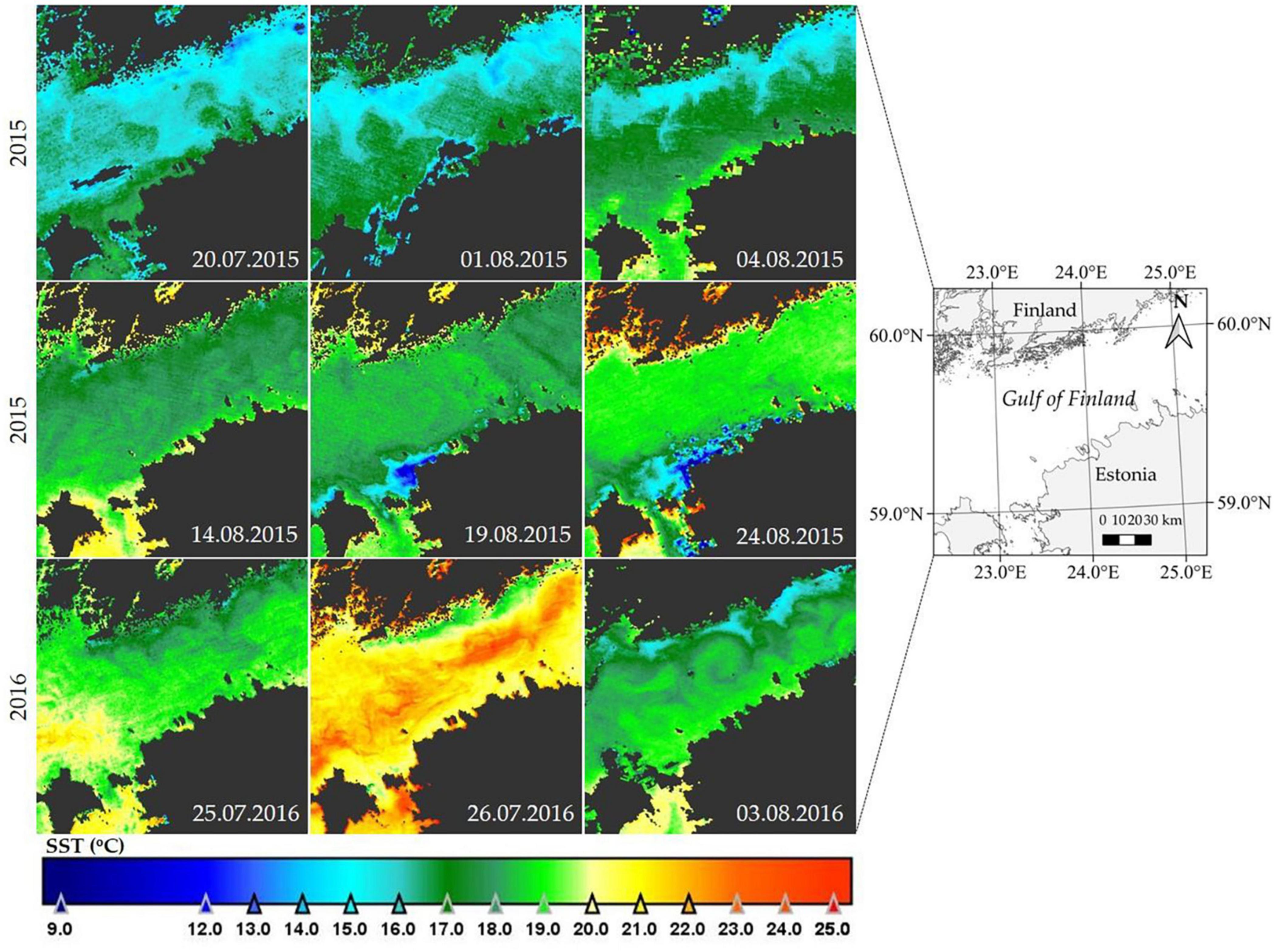
Figure 2. Sea Surface Temperature (SST) maps from MODIS data for the 2015 and 2016 monitoring period. Coastal upwelling regions with lower surface temperature can be observed.

Temperature and salinity profiles measured at filed campaigns are shown in Figure 3. There were no significant differences in the horizontal distribution of the temperature at the surface layer during different observation days. However, the vertical distribution of temperature and salinity varied considerably between the observation days. On July 20, 2015 and July 30–31, 2015 measurement cruises, the upper 25 m water column was well-mixed and the temperature and salinity profiles were almost homogeneous. Local weather data (Estonian Weather Service, 2020) revealed that before the measurement campaigns, western winds were dominant. As a result, a downwelling event occurred which caused the water column to mix up to a 25 m depth. The SST from MODIS data also show that the temperature was higher on July 20, 2015 (Figure 2) along the north-western coast of Estonia, indicating the downwelling event.

FIGURE 3

Figure 3. Vertical profiles of temperature, salinity, attenuation coefficient (c(440)), scattering coefficient (b(440)), absorption coefficient (a(440)) and b(440)/a(440) at the wavelength of 440 nm during different hydrodynamic situations: (A) mixed water column down to a 25 m depth (the vertical temperature gradient was consistently <0.1°C m^–1), (B) intermediate situation with steady vertical decrease in temperature (the vertical temperature gradient was steadily ≥0.1°C m^–1), (C) stratified profile (there was a layer with a vertical temperature gradient ≥0.1°C m^–1 under the layer where the gradients were steadily <0.1°C m^–1). The dotted line on the b(440)/a(440) graph represents the boundary from which either the absorption b(440)/a(440) < 1 or scattering b(440)/a(440) > 1 dominates. In addition, the median concentrations of chlorophyll-a (Chl-a) and total suspended matter (TSM) are given with the interquartile range.

In general, the analysis of thermohaline structure (temperature–salinity curves) revealed three different situations in terms of vertical stratification: (1) well mixed profiles down to 25 m, (2) intermediate situation (steady decrease in temperature or increase in salinity with depth), and (3) stratified profiles with distinct thermocline (clear distinction between the upper mixed layer, thermocline and the layer under the thermocline) (Figure 3). In case of the mixed profile, the vertical temperature gradient was consistently <0.1°C m^–1. In the intermediate situation, the vertical temperature gradient was steadily ≥0.1°C m^–1. In the case of stratified profiles, there was a layer with a vertical temperature gradient ≥0.1°C m^–1 under the layer where the gradients were steadily <0.1 °C m^–1. The water column profile types form the basis for the further analysis of the IOPs and AOPs.

Distribution of Inherent Optical Properties

The vertical variability of IOPs was analysed in case of three different (non)stratification conditions. At the surface layer, the measured attenuation coefficient at 440 nm (c(440)) varied between 0.94 and 7.56 m^–1. The scattering coefficient at 440 nm (b(440)) varied between 0.42 and 6.86 m^–1. The distribution of the absorption coefficient showed less variability, being 0.45 and 0.89 m^–1 at 440 nm (a(440)).

The median values of IOPs measured at the surface layer, 10 and 20 m depth in three different hydrodynamic situations are shown in Table 2. The corresponding OSC (Chl-a and TSM) are given in Table 3. The vertical distribution of IOPs coincides with the changes in thermohaline structure (Figure 3 and Table 2). The density boundary at the thermocline prevents mixing of the upper and lower water masses. As a result, the vertical transport of OSC between the water layers is impeded.

TABLE 2

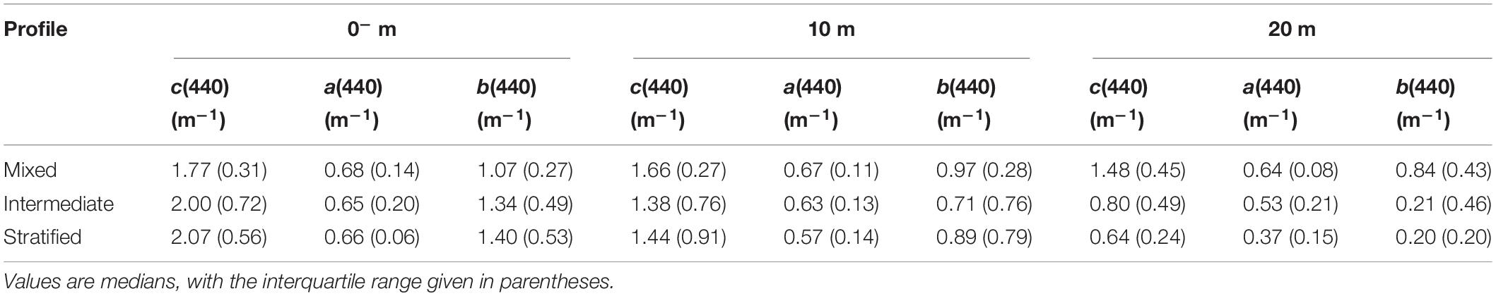
Table 2. Inherent optical properties (IOPs) such as the attenuation coefficient (c(440)), absorption coefficient (a(440)), and scattering coefficient (b(440)) at a wavelength of 440 nm for different hydrodynamic situations at different depths.

TABLE 3

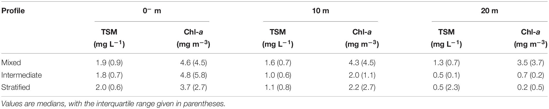
Table 3. In situ measured optically significant constituents (OSC), such as the concentration of total suspended matter (TSM) and chlorophyll-a (Chl-a) for different hydrodynamic situations at different depths.

In the case of stratified water column (Figure 3C), the vertical profiles of temperature, c(440) and b(440) were similar, and all three parameters decreased rapidly at the thermocline. For instance, the median values of c(440) and b(440) decreased by 1.43 (2.07–0.64 m^–1) units and 1.20 (1.40–0.20 m^–1) units, respectively, over the measured water column (0–25 m). Additionally, the ratio of b(440) to a(440) changed under the thermocline (b(440)/a(440) < 1), which demonstrates that absorption became the dominant component of attenuation. The correlation (r²) between median profiles of temperature and the b(440)/a(440) was 0.99. Although there were no significant changes in the vertical distribution of a(440), there was a slight shift of about 0.29 units for a(440). Below the thermocline, there were no significant changes in the IOPs down to a 25 m depth.

In the case of the intermediate situation (Figure 3B) where stratification was not so obvious, but the temperature was decreasing with depth, a similar pattern occurred as in case of the strongly stratified situation. The b(440) decreased smoothly with depth so that a(440) became dominant at a certain depth, the r² between median profiles of temperature and the b(440)/a(440) was 0.86. The medians of c(440) and b(440) decreased from the surface layer to 25 m depth by 1.20 (2–0.80 m^–1) units and 1.13 (1.34–0.21 m^–1) units, respectively. A decrease of concentrations of OSC was also observed (Table 3). The measured profiles confirm that the change in distribution of IOPs profiles reveals the change in relative concentrations of the OSC (note changes in Chl-a and TSM concentrations).

In the mixed water column (Figure 3A), there is no density boundary and the vertical variability of IOPs was very small (<0.30 units in case of c(440) and b(440) and 0.04 units for a(440)). Therefore, the ratio of b(440)/a(440) remained almost the same through the entire water column. The r² between median profiles of temperature and the b(440)/a(440) was 0.89. In addition, the vertical variability of OSC was small (Table 3 and Figure 3).

Vertical profiles of measured IOPs (Figure 3) in study area show that: (1) in the upper mixed layer scattering contributed most to attenuation, i.e., scattering dominated over the absorption; (2) the vertical distribution of the scattering coefficient coincides with the vertical distribution of the attenuation coefficient; (3) and below the density layer, absorption becomes the dominant factor in the attenuation, i.e., the ratio of b(440)/a(440) becomes lower than one in the south-western coast of Gulf of Finland.

Distribution of Simulated Apparent Optical Properties

The following analysis is based on the division of water masses by stratification of the water column. R(λ) and K_d(λ) were simulated from IOPs measured at different depths. By simulating the AOPs from IOPs for different water masses enabled to evaluate the changes in optical parameters that might occur when a water mass rises from deeper layers to the surface layer as a result of an upwelling event.

Variability of simulated R(λ) in the PAR region (400–700 nm) is shown in Figure 4A. R(λ) at 400 nm ranged from 0.31 to 3.94 units, at 550 nm from 0.92 to 12.98 units and at 700 nm from 0.31 to 5.52 units for the surface layer. R(λ) simulated from IOPs measured at 20 m depth were 0.01–1.01, 0.28–3.99, and 0.09–1.79 units depending on water mass stratification. The spectral shape of simulated R(λ) showed highest reflection in the green part of the spectrum, in particular, at 550–580 nm and lower reflection in blue and red part of the spectrum which is typical spectral shape for Case II water type. A minimum of 670 nm was also observed, which corresponds to the absorption of Chl-a. The spectra that represent water mass at a 20 m depth are considerably smoother at the longer wavelengths due to the lower particles concentrations at this depth.

FIGURE 4

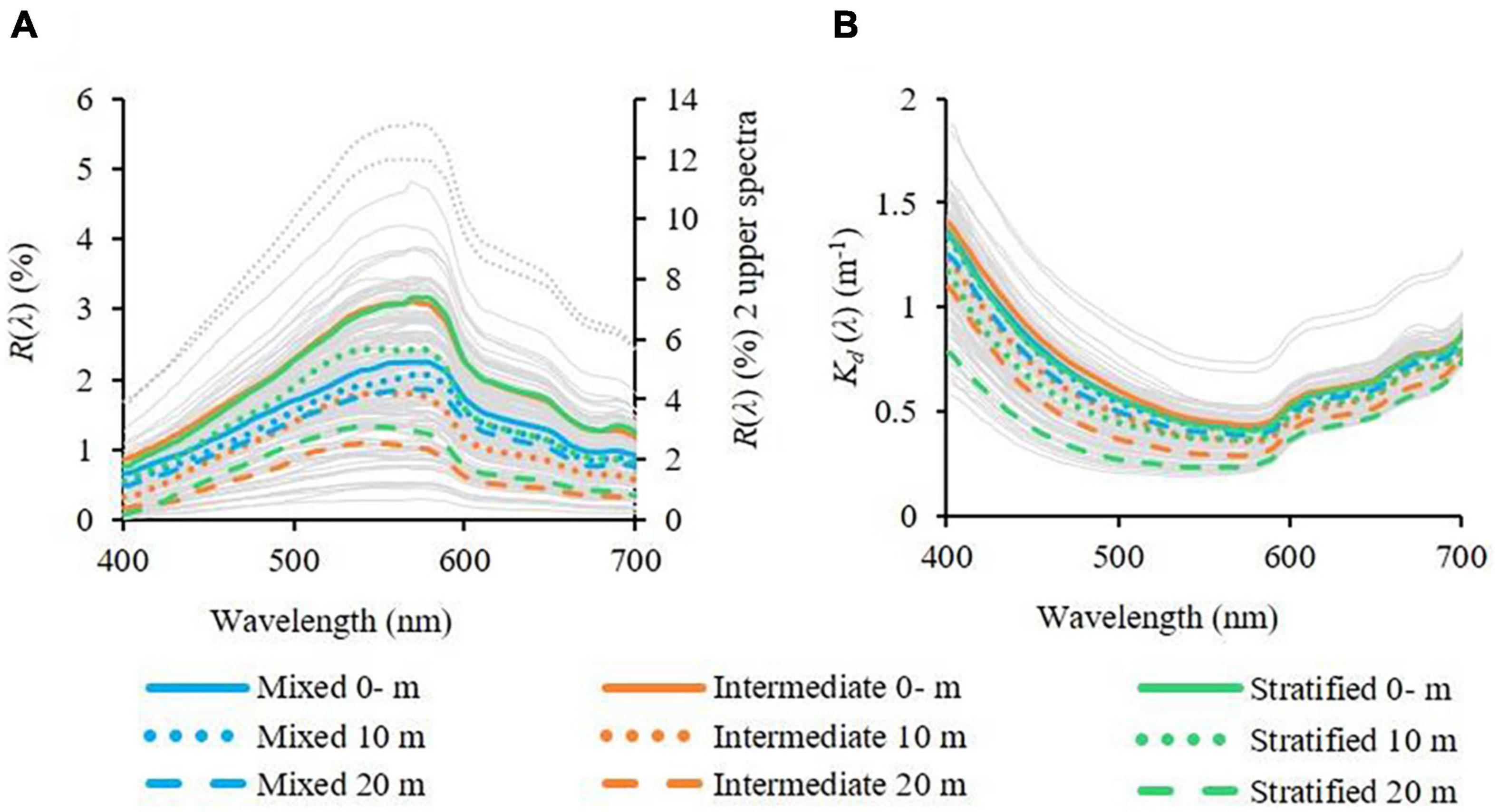
Figure 4. Vertical variability of the simulated (A) spectral irradiance reflectance (R(λ)) and (B) spectral diffuse attenuation coefficient (K_d(λ)) at 0^– m (surface layer), 10 m depth and 20 m depth. Coloured line represents the median spectra of the respective stratification situation. Note the secondary axis on panel (A) for the 2 spectra with highest values.

The K_d(λ) calculated from the a(λ) and b(λ) measurements at three depths are shown in Figure 4B. The spectral dependence of K_d(λ) curves at different depths is quite similar. However, the numerical value of K_d(λ) varied greatly and the variation was largest at shorter wavelengths (400–550 nm). It is known that, in this spectral region, Chl-a and CDOM have the main influence on the optical parameters. For instance, the greatest decrease in K_d(PAR) in one station was 40.8%, which resulted in corresponding changes in Chl-a (80.1%) and TSM (61.4%). The smallest vertical decrease of K_d(PAR) (6.8%) occurred when Chl-a and TSM decreased from the surface layer to 20 m by 31.7 and 42.1%, respectively.

Evaluation of the differences in z₉₀(λ) revealed that the thickness of the water layer, which would be detected by optical remote sensing instruments depends on the wavelength and water mass (Figure 5). It was found that the informative layer is largest in the wavelength range of 550–600 nm, where the median value of z₉₀(λ) was 2.1 m. The lowest z₉₀(λ) values were in the 400, 450, and 700 nm spectral region, where the median z₉₀(λ) values were 0.7, 1.2 and 1.2 m, respectively. However, simulations indicate that in the case of intensive coastal upwelling when water mass from deeper layers reaches the surface the z₉₀(λ) might exceed 4 m (550 nm), and values in the 400, 450, and 700 nm spectral region might be up to 1.3, 2.4, and 1.4 m, respectively.

FIGURE 5

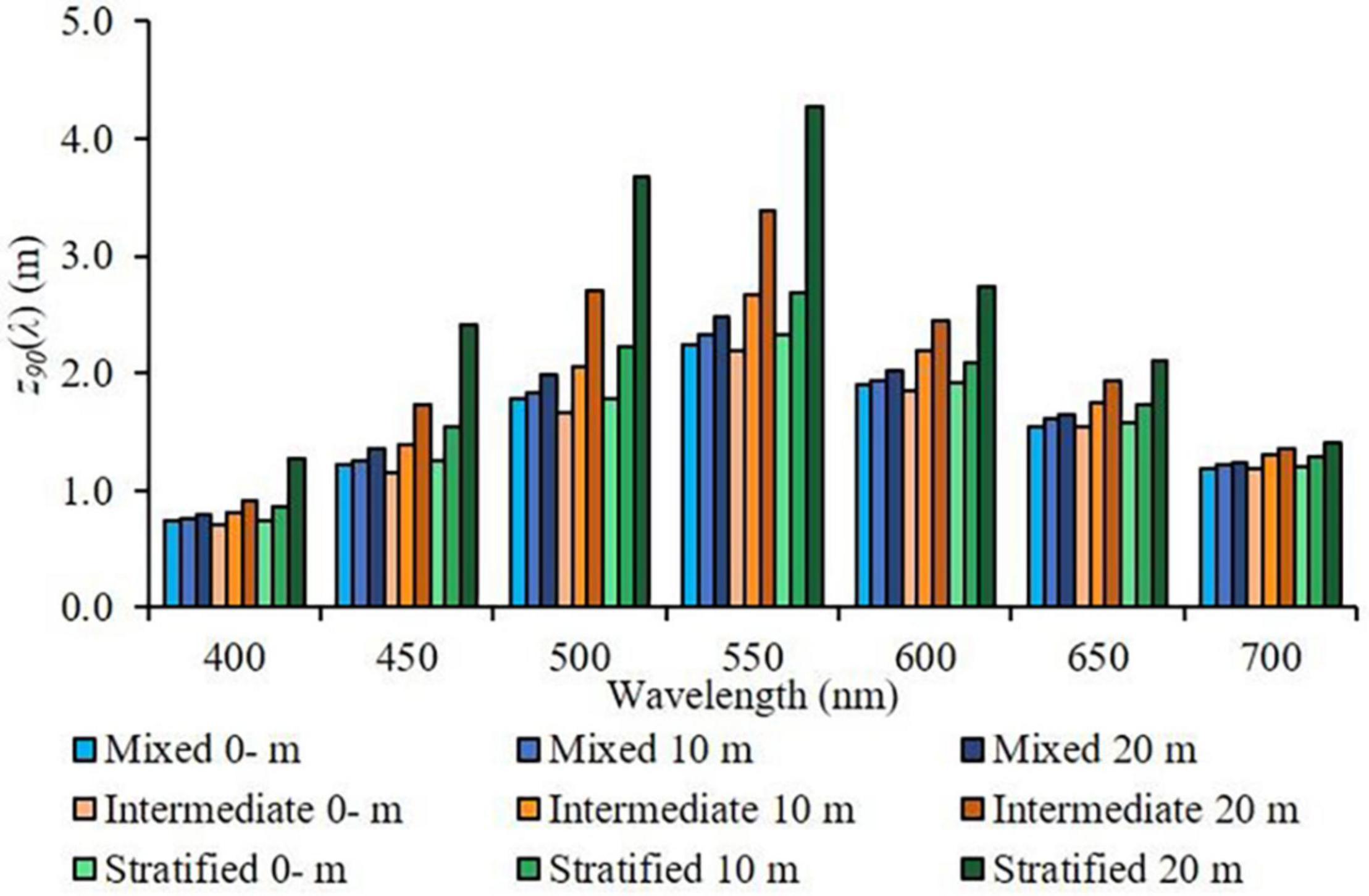
Figure 5. Spectral variability of optical depth (z₉₀(λ)) at the surface layer, 10 m depth and 20 m depth in different situations of stratification.

Detection of Upwelling Zone From Apparent Optical Properties

In section 3.3 we demonstrated the changes in R(λ) and K_d(λ) values that might occur when a water mass rises from deeper layers to the surface layer as a result of an upwelling event. Simulation indicated that K_d(PAR) decreases up to 37.5% and R(PAR) 61.5% in the subsurface layer (Table 4). The simulated results of R(λ) for different water masses were compared with measurements of R(λ) (with TriOS RAMSES radiometers) from an independent dataset collected during the upwelling event on July 4–5, 2018 (Figure 6). The strong upwelling event occurred in the region of the study area (south-western part of the Gulf of Finland). The SST dropped to 4.8°C, whereas the Secchi depth was extremely high for summer time (in the context of the Baltic Sea), with a value of 12.2 m (Figure 6). The Chl-a values measured in the upwelling zone were around 0.5 mg m^–3, which, given that the measurements were taken at the beginning of July, are rather low. On the contrary, outside the upwelling zone (two stations that were only 25–30 km from the upwelling station), the water temperature was about 15°C, the Secchi depth was 3.3–3.7 m, the concentration of Chl-a was 17.5–20.6 mg m^–3 and TSM concentration was 3.5–3.7 mg L^–1. Two different types of water mass were distinguishable from the in situ R(λ) spectra measured with Ramses instrument (Figure 6): (1) typical coastal water, which is strongly reflected in the green part of the spectrum (550–580 nm), and (2) upwelled water with considerably smoother R(λ) spectra.

TABLE 4

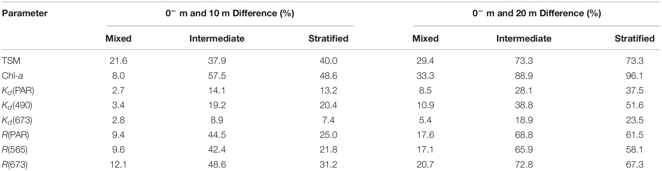
Table 4. Differences (%) between the concentration of optically significant constituents (OSC) such as the concentration of total suspended matter (TSM) and chlorophyll-a (Chl-a), and the spectral diffuse attenuation coefficient (K_d(λ)) and the spectral irradiance reflectance (R(λ)) at different wavelengths by respective depths and hydrodynamic situations.

FIGURE 6

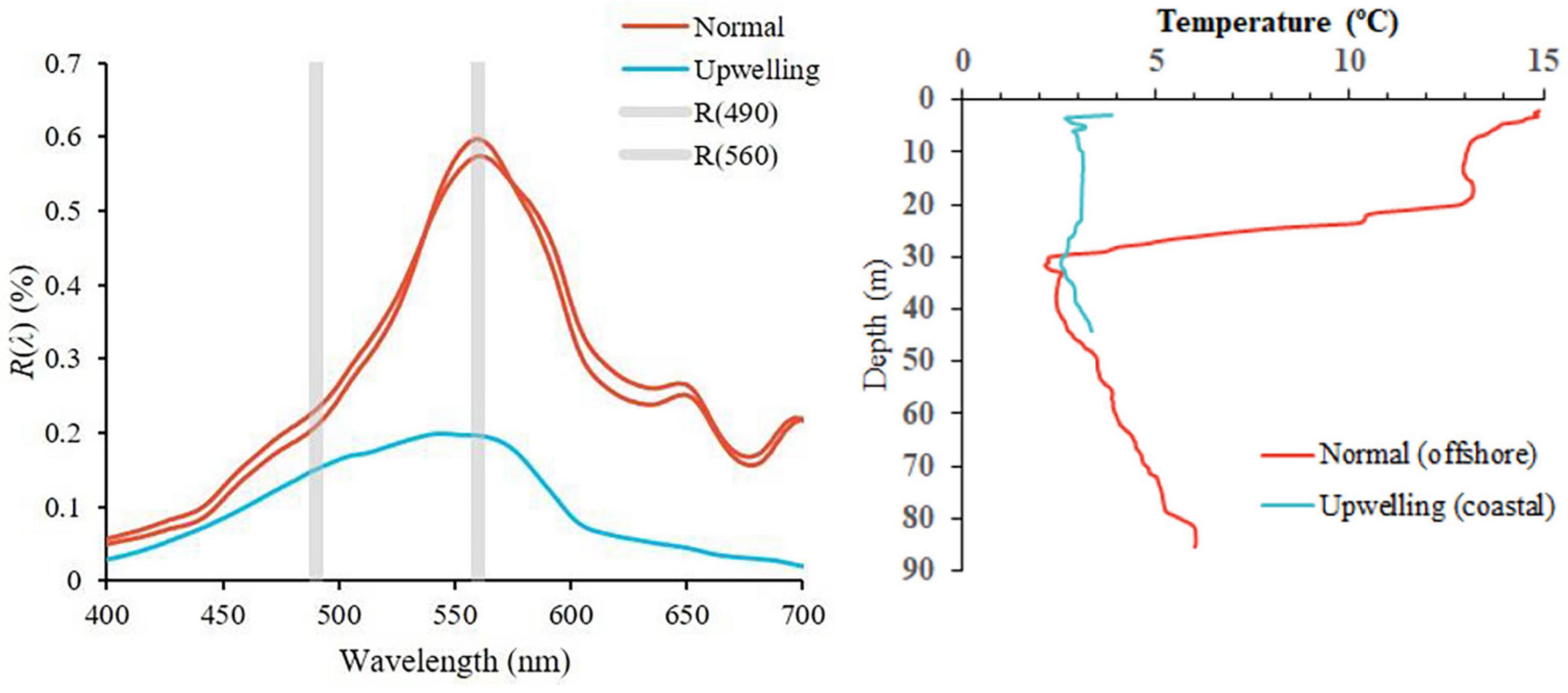
Figure 6. The spectral irradiance reflectance (R(λ)) of in situ measurements (July 4–5, 2018) with two TriOS RAMSES radiometers during upwelling and normal situations (left panel). The corresponding measured temperature profiles indicating strong coastal upwelling with surface temperature below 5°C (right panel).

Due to the difference in R(λ) spectra between the two water mass, a simple band ratio condition was tested to detect the upwelled water mass. The R(490)/R(560) value was calculated from the upwelling in situ R(λ) spectra (shown in Figure 6). Condition for the separation of upwelling zones (R(490)/R(560)≥0.77) was set ≥0.77 relying on in situ Rameses data collected on July 4–5, 2018. The characteristic spectra for upwelling and non-upwelling situations are shown in Figure 6.

We also tested the ratio condition to satellite data. Two cloud-free Sentinel-3 OLCI images acquired during intense upwelling events (July 14 and July 21, 2020) in the Gulf of Finland were chosen for testing. Figure 7 shows the combined result of the SST and band ratio condition, where the latter is marked with a black hatched area on the SST map. The SST maps (Figure 7) show large upwelling areas along the southern coast of the Gulf of Finland, where the temperatures remained below 10°C. The figure shows how the horizontal distribution of the upwelling zone based on SST coincides quite well with the area indicated on the basis of the R(λ) spectra from OLCI. Thus, the band ratio approach may be useful in order to assess whether upwelling is occurring if the SST data is not available.

FIGURE 7

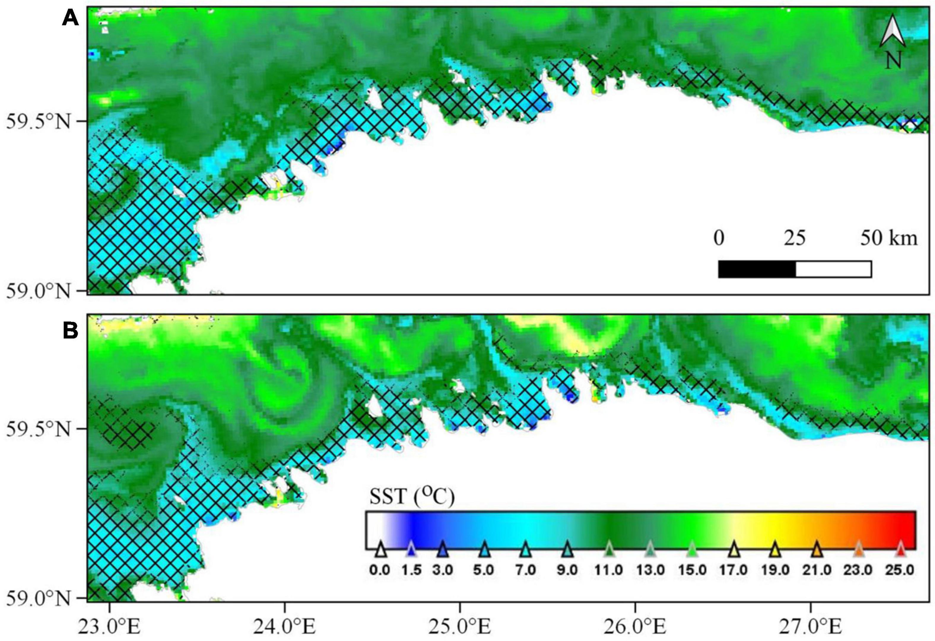
Figure 7. Sea surface Temperature (SST) maps derived from SLSTR data on (A) 14 June 2020 and (B) 21 June 2020 (Gulf of Finland). The area hatched in black indicates the condition R(490)/R(560) ≥ 0.77 fulfilled from the OLCI data from the same overpass date with the SLSTR SST data.

Discussion

The general aim of current study was to give an overview of the variation of optical parameters and the relationship of these parameters with thermohaline structure based on measurements made on the south-western coast of the Gulf of Finland. In the analysis of the IOPs distribution, the main focus was on a wavelength of 440 nm, because values close to this wavelength are used in Case-2 Regional processors to derive IOPs from remote sensing data, which are then used as a proxy for concentrations of OSC (Brockmann et al., 2016). The measurements of IOPs showed that in the upper mixed layer, the light attenuation process is mainly dominated by scattering. Sipelgas et al. (2004) also showed that the light scattering dominated over the absorption in the south-western coastal sea of the Gulf of Finland. However, they also demonstrated that in the Moonsund, which is near to our study area, where the optical properties of water are mainly influenced by the river inflow, the light absorption was found to be dominant. This discrepancy between the two studies indicates that the distribution of IOPs can change quite rapidly within a small spatial area.

The variation of OSC was moderate compared to other studies carried out in different region over the Baltic Sea. Chl-a varied between 0.36 and 15.06 mg m^–3 and TSM between 0.80 and 4.40 mg L^–1. Therefore, also, the IOPs in the surface layer did not vary much. Different studies (Woźniak et al., 2011; Sipelgas and Raudsepp, 2015; Soja-Woźniak et al., 2017; Kratzer and Moore, 2018) have showed that intensive blooms (surface scums), resuspension, and anthropogenic impact (e.g., dredging), would significantly change the distribution of OSC and IOPs in much larger scale.

However, depending on the vertical distribution of OSC in different thermohaline conditions, a significant variation in the ratio of b(440) to a(440) was observed. In the mixed water column, the ratio was more stable than in the situation when stratification occurred. With an increase of depth, the a(440) in the stratified water column became dominant in c(440). Berthon and Zibordi (2010) obtained similar vertical distributions of IOPs in the Baltic Proper, where the surface (upper mixed) layer was dominated by scattering, whereas the intensity of scattering decreased with an increasing depth and in the deeper layers absorption became more dominant. Berthon and Zibordi (2010) also showed that the optical properties of the Baltic Sea vary considerably, depending on the regional characteristics. On contrary to the Baltic Proper (closest to our study area), it was found that in the northern part of the Baltic Sea (Bothnian Bay), absorption was dominant within the upper 25 m water column. The reason for this was high absorption by CDOM resulting from the presence of humic matter brought by the numerous rivers. They found that in the Bothnian Bay, the contribution of CDOM to absorption was up to 35% higher than in the Baltic Proper. Unfortunately, CDOM concentrations were not measured in the present study, which makes it difficult to assess directly the contribution of CDOM to beam attenuation. However, previous studies (Sipelgas et al., 2004; Ylöstalo et al., 2016; HELCOM, 2018, Kratzer and Moore, 2018) have shown that Baltic Proper and western Gulf of Finland (our study area) have also high absorption of CDOM at 440 nm (up to 4.1 m^–1), but not as high as in the Bothnian Bay (up to 8.8 m^–1).

One of the reasons why the vertical distributions of optical parameters were compared was to evaluate the influence of upwelling event on the optical properties of surface water. During the development stage of an upwelling, more productive and turbid surface waters are pushed away from the shore. The water mass that rises from deeper layers of the stratified water column differs from the original water mass in terms of temperature, nutrients and OSC, which, as a result, changes the optical properties of the surface layer. For instance, Uiboupin et al. (2012) showed that in the case of an upwelling event, the area influenced by upwelled water might cover up to 40% of the total area of the Gulf of Finland in the Baltic Sea. Moreover, filaments of upwelled water may spread much farther, reaching several tens of kilometres out into the sea and in some case, cross the entire Gulf of Finland (Zhurbas et al., 2008). Several studies have demonstrated that in the case of an intensive upwelling front, the low Chl-a regions coincide with the cold upwelled water area and concentrations may drop down by an order of magnitude (Uiboupin et al., 2012; Dabuleviciene et al., 2018, 2020). The latter proves that the upwelling is an important process that, in addition to temperature changes, alters the optical signal of surface water measured by a remote sensor. Therefore, it is important to quantify the influence of upwelling water on remote sensing signal.

We quantified the change in magnitude and spectral shape of remote sensing signal in upwelling conditions by simulating the AOPs (K_d(λ) and R(λ)). Delpeche-Ellmann et al. (2018) showed that the cooler water most likely originates from intermediate water masses at depths between 15 and 30 m. In our study, AOPs (K_d(λ) and R(λ)) were calculated from the measured a(λ) and b(λ) and simulated to represent water masses at three different depths: surface layer, 10 and 20 m. It is considered that AOPs simulated from IOPs measured below the density barrier represent water masses in an upwelling condition. For instance, Lips et al. (2009) showed that during an intensive upwelling event in the central Gulf of Finland, the cold intermediate layer water was mixed with the water from the upper mixed layer, with a share of 85 and 15%, respectively. Calculations of AOPs showed that water below thermocline has substantially lower values of R(PAR), the decrease could be between 61.5 and 68.8%. The variation in the shapes of R(λ) spectra was also observed under different stratification conditions. The spectra of the deeper water layers under the thermocline had significantly less spectral dependency, R(λ) spectra were no longer representing typical coastal water, which is strongly reflected in the green part of the spectrum. Our results represent the theoretical simulations of AOPs in upwelling conditions, however in natural environment during the upwelling, waters from different layers are both advected and mixed.

Another important aspect is the significant differences in the spectral values of z₉₀(λ) under upwelling condition. Our analyses indicate that the thickness of the water layer measured by the remote sensor may increase compared to the typical coastal water condition from 2.3 to 4.3 m in the green region of the spectrum. Simis et al. (2017) demonstrated that 90% of water-leaving radiance at 560 nm exceeded 5 m if the biomass (Chl-a) was less than 5 mg m⁻³. Otherwise, the mean values of z₉₀(λ) were 1.0, 3.0–3.5, and 1.5 m, in the blue, green and red spectral region, respectively. The latter are also comparable to the results obtained in the present study. Furthermore, both studies show that the most informative spectral region for the Baltic Sea waters is located near 550–560 nm. The above analysis about variability of the z₉₀(λ) for different water masses highlights the need for an additional optical classification of waters prone to the upwelling phenomenon.

The obtained simulation results of R(λ) for different water masses were confirmed by measurements of R(λ) from an independent dataset of TriOS RAMSES radiometers collected during the upwelling event. Two different types of water masses were distinguishable (Figure 6): (1) typical coastal water which is strongly reflected at 550–580 nm and (2) upwelled water with considerably smoother R(λ) spectra. Such a difference in the shape of R(λ) spectra may have an effect on the use of algorithms to derive OSC concentrations found as a result of the classification of optical water types, where reflectance spectrum features are associated with a specific bio-optical condition. Such classification approaches are widely used in the remote sensing of water bodies (Vantrepotte et al., 2012; Shen et al., 2015; Jackson et al., 2017; Spyrakos et al., 2018; Uudeberg et al., 2019, 2020). Based on the difference in the R(λ) spectrum shapes in the current study, it is suggested that the ratios between R(490) and R(560) values can be used as an indicator for the detection of upwelled water (in this work R(490)/R(560)≥0.77). The applicability of the proposed band ratio approach was tested for discerning upwelling events in satellite imagery. Comparison of satellite SST and reflectance band ratio derived from OLCI image showed good agreement, low SST values (below 10^oC) coincided with the upwelling area indicated by the band ratio algorithm (Figure 7). Implementation of ratio condition to optical remote sensing imagery allows separating the upwelling region also from missions Sentinel-2 or Landsat which are not primarily designed for SST estimation.

The SST based approach has been widely used for monitoring upwelling events. However, the band ratio method proposed in this work offers an alternative way to estimate the pixels belonging to the upwelled water region from optical satellite images. In addition, the acquisition of optical and temperature sensors is not always simultaneous, which prevents the use of this data in synergy. For instance, Sentinel-2 satellites do not include thermal infrared sensors like Sentinel-3 and Terra/Aqua. Besides, the spatial resolution of optical sensors is often significantly higher than of the thermal infrared sensors, thus providing more detailed added value.

Previous studies have shown how biological (phytoplankton, primary production), chemical (phosphate, nitrate), and physical (temperature, salinity) patterns change at different stages of upwelling (Vahtera et al., 2005; Lips et al., 2009; Uiboupin et al., 2012), but there is no detailed information on how the optical properties of water change during upwelling in the Gulf of Finland. As there was no time series of such data in the present work, it is planned for the future to perform additional measurements and analyse how the optical properties of water change over time (before, during and after upwelling) in the Gulf of Finland region. The current study reviled the consequences of upwelling in optical properties in the Gulf of Finland. However, the conclusions cannot be automatically expanded to the other basins of the Baltic Sea as the vertical distribution of IOPs differ between basins of the Baltic Sea (Berthon and Zibordi, 2010; Soja-Woźniak et al., 2017; Kratzer and Moore, 2018). However, upwelling is a frequent process also in other basins of the Baltic Sea (Lehmann et al., 2012; Dabuleviciene et al., 2018, 2020; Bednorz et al., 2021), therefore future research is needed to quantify the effect of upwelling on the remote sensing signal/retrievals in the other basins of the Baltic Sea.

Conclusion

On the basis of IOPs, OSC (Chl-a and TSM) and vertical profiles of temperature and salinity, the optical parameters of the south-western part of the Gulf of Finland (Baltic Sea) have been investigated. The analysis of the thermohaline structure revealed three different situations in terms of vertical stratification: (1) mixed water column down to 25 m depth, (2) intermediate situation (steady decrease in temperature or increase in salinity with depth), and (3) stratified profiles with a distinct thermocline. The comparison of the vertical profiles of temperature and IOPs showed similar patterns in vertical variability. In the situation of a mixed water column, the optical parameters did not change significantly through the entire water column. In the stratified water column, the concentrations of OSC changed considerably and the vertical variability of attenuation and scattering was significantly higher compared to the mixed layer [i.e., the difference of c(440) between surface and 20 m depth was 69.1 and 16.4%, respectively]. The analysis of IOPs in the case of stratified water column showed that the ratio of scattering b(440) to absorption a(440) changed under the thermocline (b(440)/a(440) < 1) i.e., absorption became the dominant component of attenuation under thermocline while the opposite is true for upper layer. The results showed that the stratification of the water column is related to the variability of the optical parameters through the distribution of OSC.

The values of R(λ) and K_d(λ) were calculated from IOPs measured at three different depths: surface layer, 10 and 20 m. The performed simulation allow to assume how surface R(λ) values would change if upwelling events occur. The results showed that in the upwelling region, the signal measured by the remote sensor may decrease up to 68.8% as a result of deep water uptake. Additionally, the R(λ) spectra would be considerably smoother, as the strong reflection in the green part of the spectrum (550–580 nm) is diminished. Moreover, the z₉₀(λ)—the thickness of the water layer measured by the remote sensor—of upwelled water may increase from 2 to 4 m in the green part of the reflectance spectra compared to the typical coastal water of the Baltic Sea. The study also showed that the small vertical decrease of K_d(PAR) by 6.8% (from surface to 20m depth) corresponds to much larger Chl-a and TSM decreased by 31.7 and 42.1%, respectively. It is suggested that the AOPs and IOPs can be used as an indicator for the detection of upwelled water mass from remote sensing data: 1) R(490)/R(560)≥0.77); 2) b(440)/a(440) < 1. The application of ratio condition R(490)/R(560)≥0.77 to the optical imagery allows determining the upwelled water mass in more detail (spatially) than with the SST approach and is in synergy with derived ocean colour retrievals. Allowing estimation of upwelling zone independently for SST data. All these aspects show that upwelling is an important process that, in addition to temperature changes, alters the optical signal of surface water measured by a remote sensor. Knowledge of IOPs and AOPs relation to upwelling can help the parametrisation of remote sensing algorithms for retrieving water quality estimates in the coastal regions.

Data Availability Statement

The raw data supporting the conclusions of this article will be made available by the authors, without undue reservation.

Author Contributions

AA, RU, and LS: conceptualisation, methodology, software, formal analysis, data curation, visualisation, and writing—original draft preparation. AA, LS, RU, and KU: investigation and writing—review and editing.

Funding

This research was funded by the European Regional Development Fund within the National Programme for Addressing Socio-Economic Challenges through R&D (RITA1/02-52-04).

Conflict of Interest

The authors declare that the research was conducted in the absence of any commercial or financial relationships that could be construed as a potential conflict of interest.

Acknowledgments

We would like to thank the crew of R/V Salme and our colleagues from the Department of Marine Systems for helping collect the in situ data.

References

Alenius, P., Myrberg, K., and Nekrasov, A. (1998). The physical oceanography of the Gulf of Finland: a review. Boreal Environ. Res. 3, 97–125.

Google Scholar

Alenius, P., Nekrasov, A., and Myrberg, K. (2003). Variability of the baroclinic Rossby radius in the Gulf of Finland. Cont. Shelf Res. 23, 563–573. doi: 10.1016/S0278-4343(03)00004-9

CrossRef Full Text | Google Scholar

Alikas, K., Kratzer, S., Reinart, A., Kauer, T., and Paavel, B. (2015). Robust remote sensing algorithms to derive the diffuse attenuation coefficient for lakes and coastal waters. Limnol. Oceanogr. Methods 13, 402–415. doi: 10.1002/lom3.10033

CrossRef Full Text | Google Scholar

Attila, J., Kauppila, P., Kallio, K. Y., Alasalmi, H., Keto, V., Bruun, E., et al. (2018). Applicability of earth observation chlorophyll-a data in assessment of water status via MERIS — with implications for the use of OLCI sensors. Remote Sens. Environ. 212, 273–287. doi: 10.1016/j.rse.2018.02.043

CrossRef Full Text | Google Scholar

Attila, J., Koponen, S., Kallio, K., Lindfors, A., Kaitala, S., and Ylöstalo, P. (2013). MERIS Case II water processor comparison on coastal sites of the northern Baltic Sea. Remote Sens. Environ. 128, 138–149. doi: 10.1016/j.rse.2012.07.009

CrossRef Full Text | Google Scholar

Austin, R. W. (1974). “The remote sensing of spectral radiance from below the ocean surface,” in Optical Aspects of Oceanography, eds N. G. Jerlov and E. Steemann-Nielsen (New York, NY: Academic Press), 317–344.

Google Scholar

Bednorz, E., Półrolniczak, M., and Tomczyk, A. M. (2021). Regional circulation patterns inducing coastal upwelling in the Baltic Sea. Theor. Appl. Climatol. 144, 905–916. doi: 10.1007/s00704-021-03539-7

CrossRef Full Text | Google Scholar

Berthon, J. F., and Zibordi, G. (2010). Optically black waters in the northern Baltic Sea. Geophys. Res. Lett. 37:L09605. doi: 10.1029/2010GL043227

CrossRef Full Text | Google Scholar

Brockmann, C., Doerffer, R., Peters, M., Stelzer, K., Embacher, S., and Ruescas, A. (2016). “Evolution of the C2RCC neural network for Sentinel 2 and 3 for the retrieval of ocean colour products in normal and extreme optically complex waters,” in Proceedings of the Conference held Living Planet Symposium, (Prague).

Google Scholar

Dabuleviciene, T., Kozlov, I. E., Vaiciute, D., and Dailidiene, I. (2018). Remote sensing of coastal upwelling in the South-Eastern Baltic Sea: statistical properties and implications for the coastal environment. Remote Sens. 10, 1–24. doi: 10.3390/rs10111752

CrossRef Full Text | Google Scholar

Dabuleviciene, T., Vaiciute, D., and Kozlov, I. E. (2020). Chlorophyll-a variability during upwelling events in the south-eastern baltic sea and in the curonian lagoon from satellite observations. Remote Sens. 12:3661. doi: 10.3390/rs12213661

CrossRef Full Text | Google Scholar

Delpeche-Ellmann, N., Soomere, T., and Kudryavtseva, N. (2018). The role of nearshore slope on cross-shore surface transport during a coastal upwelling event in Gulf of Finland, Baltic Sea. Estuar. Coast. Shelf Sci. 209, 123–135. doi: 10.1016/j.ecss.2018.03.018

CrossRef Full Text | Google Scholar

ESTHub Services (2020). ESTHub Satellite Data. Available online at: https://geoportaal.maaamet.ee/eng/Services/ESTHub-Services-p654.html (Accessed October 15, 2020).

Google Scholar

Estonian Weather Service (2020). Sea Weather. Available online at: https://www.ilmateenistus.ee/meri/vaatlusandmed/kogu-rannik/kaart/?lang=en [Accessed August 4, 2020].

Google Scholar

Gasinaite, Z. R., Cardoso, A. C., Heiskanen, A. S., Henriksen, P., Kauppila, P., Olenina, I., et al. (2005). Seasonality of coastal phytoplankton in the Baltic Sea: influence of salinity and eutrophication. Estuar. Coast. Shelf Sci. 65, 239–252. doi: 10.1016/j.ecss.2005.05.018

CrossRef Full Text | Google Scholar

Gidhagen, L. (1987). Coastal upwelling in the Baltic Sea-Satellite and in situ measurements of sea-surface temperatures indicating coastal upwelling. Estuar. Coast. Shelf Sci. 24, 449–462. doi: 10.1016/0272-7714(87)90127-2

CrossRef Full Text | Google Scholar

Glasgow, H. B., Burkholder, J. A. M., Reed, R. E., Lewitus, A. J., and Kleinman, J. E. (2004). Real-time remote monitoring of water quality: a review of current applications, and advancements in sensor, telemetry, and computing technologies. J. Exp. Mar. Biol. Ecol. 300, 409–448. doi: 10.1016/j.jembe.2004.02.022

CrossRef Full Text | Google Scholar

Gordon, H. R. (1988). A semianalytic radiance model of ocean color. J. Geophys. Res. 93, 10909–10924. doi: 10.1029/JD093iD09p10909

CrossRef Full Text | Google Scholar

Gordon, H. R., and McCluney, W. R. (1975). Estimation of the depth of sunlight penetration in the sea for remote sensing. Appl. Opt. 14:413. doi: 10.1364/ao.14.000413

PubMed Abstract | CrossRef Full Text | Google Scholar

Gordon, H. R., Brown, O. B., and Jacobs, M. M. (1975). Computed relationships between the inherent and apparent optical properties of a flat homogeneous ocean. Appl. Opt. 14:417. doi: 10.1364/ao.14.000417

PubMed Abstract | CrossRef Full Text | Google Scholar

Gurova, E., Lehmann, A., and Ivanov, A. (2013). Upwelling dynamics in the Baltic Sea studied by a combined SAR/infrared satellite data and circulation model analysis. Oceanologia 55, 687–707. doi: 10.5697/oc.55-3.687

CrossRef Full Text | Google Scholar

Haapala, J., and Alenius, P. (1994). Temperature and salinity statistics for the northern Baltic Sea 1961–1990. Finn. Mar. Res. 262, 51–121.

Google Scholar

HELCOM (2015). Updated Fifth Baltic Sea Pollution Load Compilation (PLC-5.5). Balt. Sea Environ. Proc. 145. 143. Available online at: http://www.helcom.fi (Accessed October 14, 2020)

Google Scholar

HELCOM (2018). Water Clarity. HELCOM Core Indic. Rep. Available online at: https://helcom.fi/media/core indicators/Water-clarity-HELCOM-core-indicator-2018.pdf (Accessed June 7, 2020).

Google Scholar

Herlevi, A. (2002). A study of scattering, backscattering and a hyperspectral reflectance model for boreal waters. Geophysica 38, 113–132.

Google Scholar

Hjerne, O., Hajdu, S., Larsson, U., Downing, A., and Winder, M. (2019). Climate driven changes in timing, composition and size of the Baltic Sea phytoplankton spring bloom. Front. Mar. Sci. 6:482. doi: 10.3389/fmars.2019.00482

CrossRef Full Text | Google Scholar

Jaanus, A., Andersson, A., Olenina, I., Toming, K., and Kaljurand, K. (2011). Changes in phytoplankton communities along a north-south gradient in the Baltic Sea between 1990 and 2008. Boreal Environ. Res. 16, 191–208.

Google Scholar

Jackson, T., Sathyendranath, S., and Mélin, F. (2017). An improved optical classification scheme for the Ocean colour essential climate variable and its applications. Remote Sens. Environ. 203, 152–161. doi: 10.1016/j.rse.2017.03.036

CrossRef Full Text | Google Scholar

Kahru, M., Håkansson, B., and Rud, O. (1995). Distributions of the sea-surface temperature fronts in the Baltic Sea as derived from satellite imagery. Cont. Shelf Res. 15, 663–679. doi: 10.1016/0278-4343(94)E0030-P

CrossRef Full Text | Google Scholar

Kikas, V., and Lips, U. (2016). Upwelling characteristics in the Gulf of Finland (Baltic Sea) as revealed by Ferrybox measurements in 2007-2013. Ocean Sci. 12, 843–859. doi: 10.5194/os-12-843-2016

CrossRef Full Text | Google Scholar

Kirk, J. T. O. (1984). Dependence of relationship between inherent and apparent optical properties of water on solar altitude. Limnol. Oceanogr. 29, 350–356. doi: 10.4319/lo.1984.29.2.0350

CrossRef Full Text | Google Scholar

Kirk, J. T. O. (2010). Light and Photosynthesis in Aquatic Ecosystems, 3rd Edn. Cambridge: Cambridge University Press.

Google Scholar

Kowalczuk, P., Stedmon, C. A., and Markager, S. (2006). Modeling absorption by CDOM in the Baltic Sea from season, salinity and chlorophyll. Mar. Chem. 101, 1–11. doi: 10.1016/j.marchem.2005.12.005

CrossRef Full Text | Google Scholar

Kownacka, J., Busch, S., Göbel, J., Gromisz, S., Hällfors, H., Höglander, H., et al. (2018). Cyanobacteria Biomass 1990-2018. HELCOM Balt. Sea Environ. Fact Sheets 2018. Available online at: http://www.helcom.fi/baltic-sea-trends/environment-fact-sheets/eutrophication/cyanobacteria-biomass/ (Accessed June 7, 2020)

Google Scholar

Kratzer, S., and Moore, G. (2018). Inherent optical properties of the Baltic Sea in comparison to other seas and oceans. Remote Sens. 10:418. doi: 10.3390/rs10030418

CrossRef Full Text | Google Scholar

Kratzer, S., and Tett, P. (2009). Using bio-optics to investigate the extent of coastal waters: a Swedish case study. Hydrobiologia 629, 169–186. doi: 10.1007/s10750-009-9769-x

CrossRef Full Text | Google Scholar

Kutser, T. (2004). Quantitative detection of chlorophyll in cyanobacterial blooms by satellite remote sensing. Limnol. Oceanogr. 49, 2179–2189. doi: 10.4319/lo.2004.49.6.2179

CrossRef Full Text | Google Scholar

Kuvaldina, N., Lips, I., Lips, U., and Liblik, T. (2010). The influence of a coastal upwelling event on chlorophyll a and nutrient dynamics in the surface layer of the Gulf of Finland, Baltic Sea. Hydrobiologia 639, 221–230. doi: 10.1007/s10750-009-0022-4

CrossRef Full Text | Google Scholar

Kyryliuk, D., and Kratzer, S. (2019). Summer distribution of total suspended matter across the Baltic Sea. Front. Mar. Sci. 5:504. doi: 10.3389/fmars.2018.00504

CrossRef Full Text | Google Scholar

Laanemets, J., Zhurbas, V., Elken, J., and Vahtera, E. (2009). Dependence of upwelling-mediated nutrient transport on wind forcing, bottom topography and stratification in the Gulf of Finland: model experiments. Boreal Environ. Res. 14, 213–225.

Google Scholar

Lehmann, A., Myrberg, K., and Höflich, K. (2012). A statistical approach to coastal upwelling in the Baltic Sea based on the analysis of satellite data for 1990-2009. Oceanologia 54, 369–393. doi: 10.5697/oc.54-3.369

CrossRef Full Text | Google Scholar

Leppäranta, M., and Myrberg, K. (2009). Physical Oceanography of the Baltic Sea. Berlin: Springer-Verlag.

Google Scholar

Liblik, T., and Lips, U. (2011). Characteristics and variability of the vertical thermohaline structure in the Gulf of Finland in summer. Boreal Environ. Res. 16, 73–83.

Google Scholar

Ligi, M., Kutser, T., Kallio, K., Attila, J., Koponen, S., Paavel, B., et al. (2017). Testing the performance of empirical remote sensing algorithms in the Baltic Sea waters with modelled and in situ reflectance data. Oceanologia 59, 57–68. doi: 10.1016/j.oceano.2016.08.002

CrossRef Full Text | Google Scholar

Lips, I., Lips, U., and Liblik, T. (2009). Consequences of coastal upwelling events on physical and chemical patterns in the central Gulf of Finland (Baltic Sea). Cont. Shelf Res. 29, 1836–1847. doi: 10.1016/j.csr.2009.06.010

CrossRef Full Text | Google Scholar

Lorenzen, C. J. (1967). Determination of chlorophyll and pheo-pigments: spectrophotometric equations. Limnol. Oceanogr. 12, 343–346. doi: 10.4319/lo.1967.12.2.0343

CrossRef Full Text | Google Scholar

Morel, A., and Gentili, B. (1993). Diffuse reflectance of oceanic waters II Bidirectional aspects. Appl. Opt. 32:6864. doi: 10.1364/ao.32.006864

PubMed Abstract | CrossRef Full Text | Google Scholar

Morel, A., and Prieur, L. (1977). Analysis of variations in ocean color. Limnol. Oceanogr. 22, 709–722. doi: 10.4319/lo.1977.22.4.0709

CrossRef Full Text | Google Scholar

Mueller, J. L. (2003). “In-water radiometric profile measurements and data analysis protocol,” in Ocean Optics Protocols for Satellite Ocean Color Sensor Validation, Revision 4, Volume III: Radiometric Measurements and Data Analysis Protocols, eds J. L. Mueller, G. S. Fargion, and C. R. McClain (Greenbelt, MD: NASA Technical Memorandum), 7–20.

Google Scholar

Mueller, J. L., Bidigare, R. R., Trees, C., Balch, W. M., Dore, J., Drapeau, D. T., et al. (2003). Ocean Optics Protocols for Satellite Ocean Color Sensor Validation, Revision 5, Volume V: Biogeochemical and Bio-Optical Measurements and Data Analysis Protocols. Greenbelt, MD: NASA Technical Memorandum.

Google Scholar

Myrberg, K., and Andrejev, O. (2003). Main upwelling regions in the Baltic Sea - a statistical analysis based on three-dimensional modelling. Boreal Environ. Res. 8, 97–112.

Google Scholar

NASA’s OceanColor Web (2020). Ocean Color Feature. Available online at: https://oceancolor.gsfc.nasa.gov/ (Accessed October 14, 2020).

Google Scholar

Nowacki, J., Matciak, M., Szymelfenig, M., and Kowalewski, M. (2009). Upwelling characteristics in the Puck Bay (the Baltic Sea). Oceanol. Hydrobiol. Stud. 38, 3–16. doi: 10.2478/v10009-009-0014-8

CrossRef Full Text | Google Scholar

Omstedt, A., Elken, J., Lehmann, A., Leppäranta, M., Meier, H. E. M., Myrberg, K., et al. (2014). Progress in physical oceanography of the Baltic Sea during the 2003-2014 period. Prog. Oceanogr. 128, 139–171. doi: 10.1016/j.pocean.2014.08.010

CrossRef Full Text | Google Scholar

Papadopoulou, A., Drakopoulos, P. G., Karageorgis, A. P., Spyridakis, N., Psarra, S., Banks, A. C., et al. (2015). “Estimation of temperature, salinity and scattering corrections of inherent optical properties using the AC-S in-situ spectrophotometer,” in Proceedings 11th Panhellenic Symposium Oceanography and Fisheries, (Mytilene), 829–832.

Google Scholar

Reinart, A., and Kutser, T. (2006). Comparison of different satellite sensors in detecting cyanobacterial bloom events in the Baltic Sea. Remote Sens. Environ. 102, 74–85. doi: 10.1016/j.rse.2006.02.013

CrossRef Full Text | Google Scholar

Ritchie, J. C., Zimba, P. V., and Everitt, J. H. (2003). Remote sensing techniques to assess water quality. Photogramm. Eng. Remote Sensing 69, 695–704. doi: 10.14358/PERS.69.6.695

CrossRef Full Text | Google Scholar

Sea-Bird Scientific (2020). ac-s Spectral Absorption and Attenuation Sensor. Available online at: https://www.seabird.com/transmissometers/ac-s-spectral-absorption-and-attenuation-sensor/family?productCategoryId=54627869911 (Accessed August 6, 2020)

Google Scholar

Shen, Q., Li, J., Zhang, F., Sun, X., Li, J., Li, W., et al. (2015). Classification of several optically complex waters in China using in situ remote sensing reflectance. Remote Sens. 7, 14731–14756. doi: 10.3390/rs71114731

CrossRef Full Text | Google Scholar

Simis, S. G. H., Ylöstalo, P., Kallio, K. Y., Spilling, K., and Kutser, T. (2017). Contrasting seasonality in opticalbiogeochemical properties of the Baltic Sea. PLoS One 12:e0173357. doi: 10.1371/journal.pone.0173357

PubMed Abstract | CrossRef Full Text | Google Scholar

Sipelgas, L., and Raudsepp, U. (2015). Comparison of hyperspectral measurements of the attenuation and scattering coefficients spectra with modeling results in the north-eastern Baltic Sea. Estuar. Coast. Shelf Sci. 165, 1–9. doi: 10.1016/j.ecss.2015.08.008

CrossRef Full Text | Google Scholar

Sipelgas, L., Arst, H., Raudsepp, U., Kõuts, T., and Lindfors, A. (2004). Optical properties of coastal waters of northwestern Estonia: in situ measurements. Boreal Environ. Res. 9, 447–456.

Google Scholar

Sipelgas, L., Uiboupin, R., Arikas, A., and Siitam, L. (2018). Water quality near Estonian harbours in the Baltic Sea as observed from entire MERIS full resolution archive. Mar. Pollut. Bull. 126, 565–574. doi: 10.1016/j.marpolbul.2017.09.058

PubMed Abstract | CrossRef Full Text | Google Scholar

Soja-Woźniak, M., Craig, S. E., Kratzer, S., Wojtasiewicz, B., Darecki, M., and Jones, C. T. (2017). A novel statistical approach for ocean colour estimation of inherent optical properties and cyanobacteria abundance in optically complex waters. Remote Sens. 9:343. doi: 10.3390/rs9040343

CrossRef Full Text | Google Scholar

Soomere, T., Bishop, S. R., Viška, M., and Räämet, A. (2015). An abrupt change in winds that may radically affect the coasts and deep sections of the Baltic Sea. Clim. Res. 62, 163–171. doi: 10.3354/cr01269

CrossRef Full Text | Google Scholar

Spyrakos, E., O’Donnell, R., Hunter, P. D., Miller, C., Scott, M., Simis, S. G. H., et al. (2018). Optical types of inland and coastal waters. Limnol. Oceanogr. 63, 846–870. doi: 10.1002/lno.10674

CrossRef Full Text | Google Scholar

Strickland, J. D., and Parsons, T. R. (1972). A Practical Handbook of Seawater Analysis, 2nd Edn. Ottawa: Fisheries Research Board of Canada.

Google Scholar

Suursaar, Ü, and Aps, R. (2007). Spatio-temporal variations in hydro-physical and -chemical parameters during a major upwelling event off the southern coast of the Gulf of Finland in summer 2006. Oceanologia 49, 209–228.

Google Scholar

Toming, K., Kutser, T., Uiboupin, R., Arikas, A., Vahter, K., and Paavel, B. (2017). Mapping water quality parameters with Sentinel-3 ocean and land colour instrument imagery in the Baltic Sea. Remote Sens. 9:1070. doi: 10.3390/rs9101070

CrossRef Full Text | Google Scholar

Uiboupin, R., and Laanemets, J. (2009). Upwelling characteristics derived from satellite sea surface temperature data in the Gulf of Finland, Baltic sea. Boreal Environ. Res. 14, 297–304.

Google Scholar

Uiboupin, R., Laanemets, J., Sipelgas, L., Raag, L., Lips, I., and Buhhalko, N. (2012). Monitoring the effect of upwelling on the chlorophyll a distribution in the gulf of Finland (Baltic Sea) using remote sensing and in situ data. Oceanologia 54, 395–419. doi: 10.5697/oc.54-3.395

CrossRef Full Text | Google Scholar

Uudeberg, K., Aavaste, A., Kõks, K.-L., Ansper, A., Uusõue, M., Kangro, K., et al. (2020). Optical water type guided approach to estimate optical water quality parameters. Remote Sens. 12:931. doi: 10.3390/rs12060931

CrossRef Full Text | Google Scholar

Uudeberg, K., Ansko, I., Põru, G., Ansper, A., and Reinart, A. (2019). Using opticalwater types to monitor changes in optically complex inland and coastalwaters. Remote Sens. 11:2297. doi: 10.3390/rs11192297

CrossRef Full Text | Google Scholar

Vahtera, E., Laanemets, J., Pavelson, J., Huttunen, M., and Kononen, K. (2005). Effect of upwelling on the pelagic environment and bloom-forming cyanobacteria in the western Gulf of Finland, Baltic Sea. J. Mar. Syst. 58, 67–82. doi: 10.1016/j.jmarsys.2005.07.001

CrossRef Full Text | Google Scholar

Väli, G., Zhurbas, V., Laanemets, J., and Elken, J. (2011). Simulation of nutrient transport from different depths during an upwelling event in the Gulf of Finland. Oceanologia 53, 431–448. doi: 10.5697/oc.53-1-TI.431

CrossRef Full Text | Google Scholar

Vantrepotte, V., Loisel, H., Dessailly, D., and Mériaux, X. (2012). Optical classification of contrasted coastal waters. Remote Sens. Environ. 123, 306–323. doi: 10.1016/j.rse.2012.03.004

CrossRef Full Text | Google Scholar

Vazyulya, S., Khrapko, A., Kopelevich, O., Burenkov, V., Eremina, T., and Isaev, A. (2014). Regional algorithms for the estimation of chlorophyll and suspended matter concentration in the Gulf of Finland from MODIS-Aqua satellite data. Oceanologia 56, 737–756. doi: 10.5697/oc.56-4.737

CrossRef Full Text | Google Scholar

Wasmund, N. (1994). Phytoplankton periodicity in a eutrophic coastal water of the Baltic Sea. Int. Rev. Hydrobiol. 79, 259–285. doi: 10.1002/iroh.19940790212

CrossRef Full Text | Google Scholar

WETLabs (2011). ac Meter Protocol Document. Revision Q. Available online at: www.wetlabs.com (Accessed April 3, 2021)

Google Scholar

Woźniak, S. B., Meler, J., Lednicka, B., Zdun, A., and Stoń-Egiert, J. (2011). Inherent optical properties of suspended particulate matter in the southern Baltic Sea. Oceanologia 53, 691–729. doi: 10.5697/oc.53-3.691

CrossRef Full Text | Google Scholar

Ylöstalo, P., Seppälä, J., Kaitala, S., Maunula, P., and Simis, S. (2016). Loadings of dissolved organic matter and nutrients from the Neva River into the Gulf of Finland – Biogeochemical composition and spatial distribution within the salinity gradient. Mar. Chem. 186, 58–71. doi: 10.1016/j.marchem.2016.07.004

CrossRef Full Text | Google Scholar

Zhurbas, V., Laanemets, J., and Vantera, E. (2008). Modeling of the mesoscale structure of coupled upwelling/downwelling events and the related input of nutrients to the upper mixed layer in the Gulf of Finland, Baltic Sea. J. Geophys. Res. Ocean 113, 1–8. doi: 10.1029/2007JC004280

CrossRef Full Text | Google Scholar