Application of Three Deep Learning Schemes Into Oceanic Eddy Detection

Recent years have witnessed the increase in applications of artificial intelligence (AI) into the detection of oceanic features. Oceanic eddies, ubiquitous in the global ocean, are important in the transport of materials and energy. A series of eddy detection schemes based on oceanic dynamics have been developed while the AI-based eddy identification scheme starts to be reported in literature. In the present study, to find out applicable AI-based schemes in eddy detection, three AI-based algorithms are employed in eddy detection, including the pyramid scene parsing network (PSPNet) algorithm, the DeepLabV3+ algorithm and the bilateral segmentation network (BiSeNet) algorithm. To justify the AI-based eddy detection schemes, the results are compared with one dynamic-based eddy detection method. It is found that more eddies are identified using the three AI-based methods. The three methods’ results are compared in terms of the numbers, sizes and lifetimes of detected eddies. In terms of eddy numbers, the PSPNet algorithm identifies the largest number of ocean eddies among the three AI-based methods. In terms of eddy sizes, the BiSeNet can find more large-scale eddies than the two other methods, because the Spatial Path is introduced into the algorithm to avoid destroying the eddy edge information. Regarding eddy lifetimes, the DeepLabV3+ cannot track longer lifetimes of ocean eddies.

Introduction

Oceanic eddies are ubiquitous in the global ocean. They play an important role in material and energy transport, and global climate changes. On a global scale, oceanic mesoscale eddies contribute significantly to horizontal heat and salt transports (Dong et al., 2014; Moreau et al., 2017; Patel et al., 2019, 2020). Many eddies identification methods based on different kinds of remote sensing data have been developed (Chelton et al., 2007; Chaigneau et al., 2008; Nencioli et al., 2010; Dong et al., 2011a,b; Faghmous et al., 2012; Chen et al., 2016).

Deep learning schemes have been used in oceanic eddies detection during the past few years. Lguensat et al. (2017) firstly applied a deep learning algorithm based on the encoder-decoder network to oceanic eddies detection in the classic framework of the semantic segmentation. The encoder-decoder network with the simple convolution module and the upsampling module was also used to detect and track oceanic eddies (Franz et al., 2018). Based on synthetic aperture radar images, deep learning was applied to automatically detect oceanic eddies according to the extracted higher-level features and fused multi-scale features (Du et al., 2019). Xu et al. (2019) applied the pyramid scene parsing network (PSPNet) to identify oceanic eddies and find that the PSPNet has great advantage in the detection of small-scale eddies. Duo et al. (2019) proposed an Ocean Eddy Detection Net (OEDNet) based on an object detection network to recognize the eddy field by enhancing the accurate small sample data to obtain the training dataset.

Systematic comparison of the performances of these AI-based methods discussed above is required to justify which one is the most applicable in eddy detection. Such comparison can also shed light on the application of AI algorithms into oceanography. The present study employs three different AI-based algorithms into eddy detection, including Pyramid Scene Parsing Network (PSPNet), DeepLabV3+ and Bilateral Segmentation Network (BiSeNet), and makes the comparisons of their results based on a few eddy parameters, such as eddy number, size and lifetime.

Materials and Methods

Pyramid Scene Parsing Network (PSPNet)

The PSPNet (Zhao et al., 2017) incorporates the pyramid pooling module (He et al., 2014) and the reduced convolution (Yu and Koltun, 2016), which fully uses the global scene to capture more details of the context information between the different category labels. Sea surface height anomaly (SSHA) data labeled with eddy information are used as the training data. Figure 1 shows the configuration of the PSPNet. A 101-level ResNet (ResNet101) model with a dilated network strategy (Yu and Koltun, 2016; Chen et al., 2017) is implemented to an input SSHA image to extract the feature map at different levels. The final feature map is reduced to 1/8 of the input image. The pyramid pooling module is then employed to obtain context information. A four-level pyramid fuses the images at the different sizes as the global prior. The prior is connected to the original feature and a convolution layer to generate the final prediction. The PSPNet program, proposed by Zhao et al. (2017), is publicly available at https://github.com/hszhao/PSPNet.

FIGURE 1

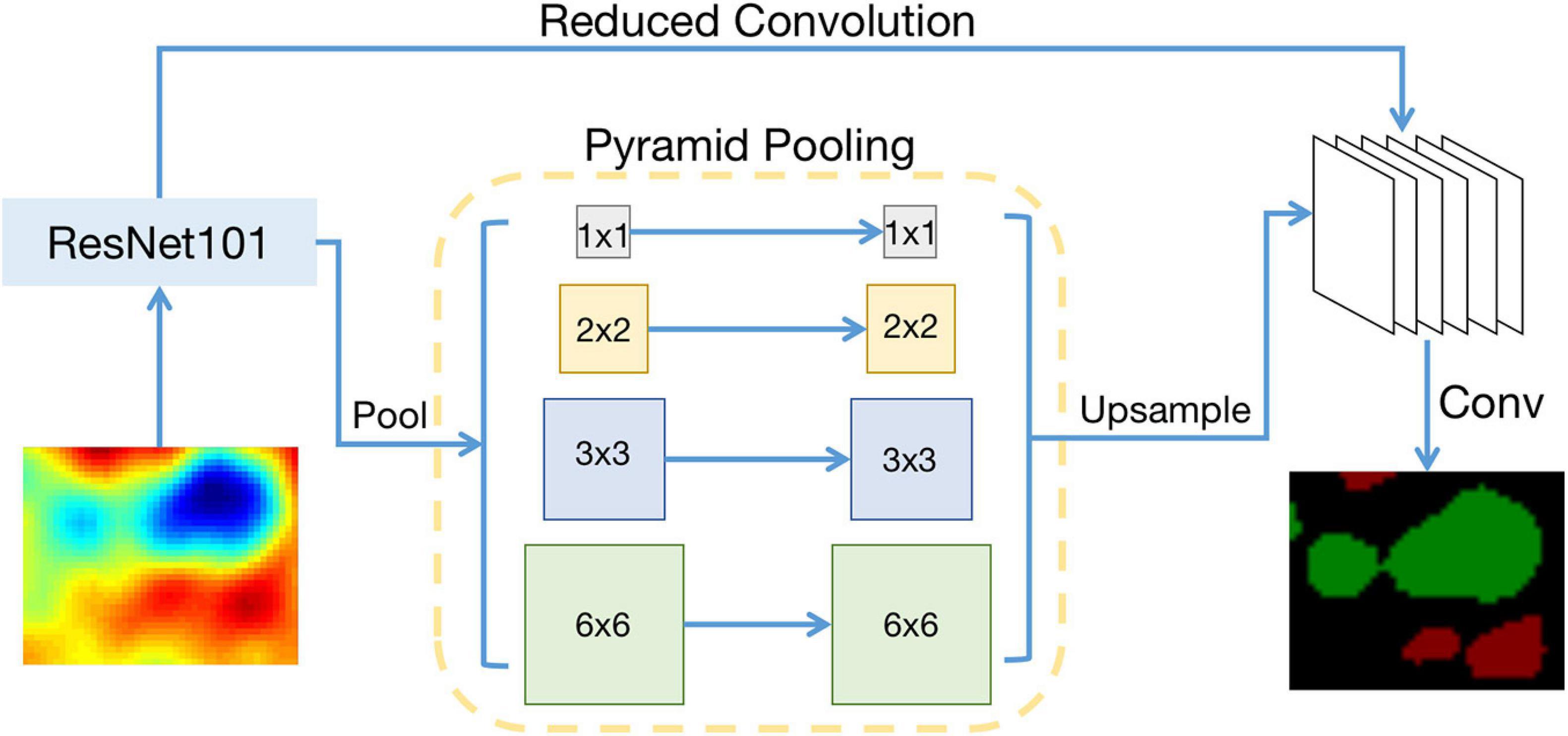
Figure 1. Schematic diagram of PSPNet.

DeepLabV3+

The DeepLabv3+ (Chen et al., 2017) employs the Spatial Pyramid Pooling module (SPP) and the encoder-decoder structure for the semantic segmentation based on the deep-learning network (Figure 2). SPP applies atrous convolution with different rates to obtain convolutional features at multiple scales to mine the multi-scale context information. The low-level features of the encoder are able to capture larger spatial information. The spatial information is used to recover the details and spatial dimensions of the target during the decoder stage, and to refine the segmentation results along object boundaries. The DeepLabV3+ program, proposed by Chen et al. (2017), can be obtained from https://github.com/tensorflow/models/tree/master/research/deeplab.

FIGURE 2

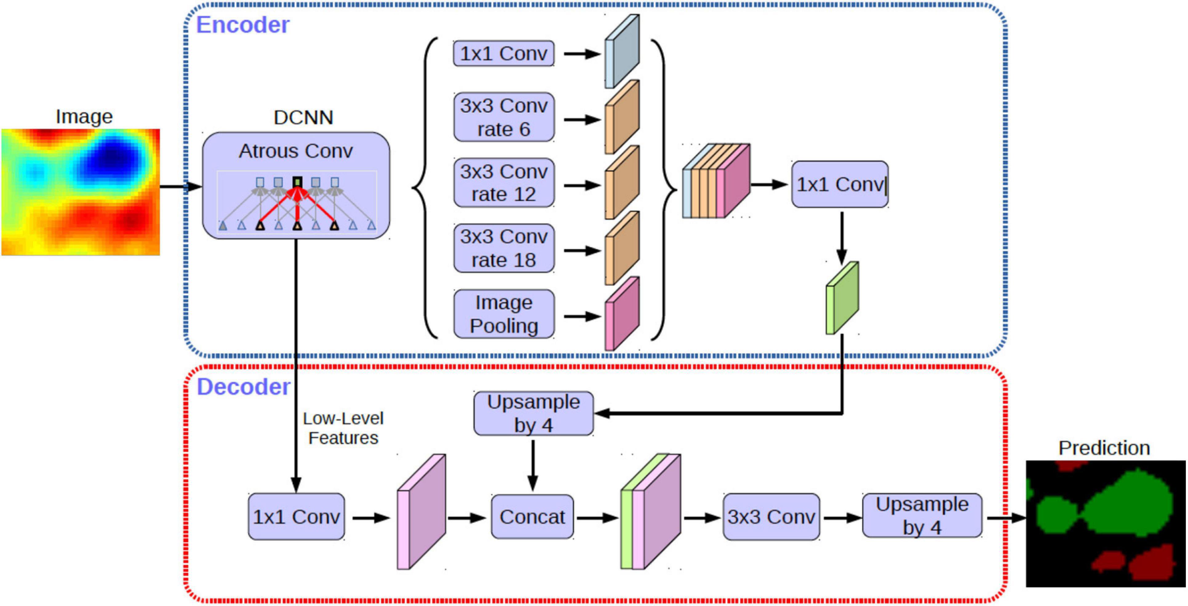
Figure 2. Schematic diagram of DeepLab V3+.

Bilateral Segmentation Network (BiSeNet)

The BiSeNet (Yu et al., 2018) is divided into three parts: Spatial Path, Context Path, and Feature Fusion Module, as shown in Figure 3. The Spatial Path encodes the detailed information captured from the image into spatial information. The Context Path is applied to encode the context information and the Feature Fusion Module is used to fuse the spatial information and the context information. According to the characteristics of the different levels, the spatial and the context information are connected in series, and a batch normalization is adopted to balance the feature information scale. The connected features are applied to obtain a weight vector employed to select and combine the feature information, and to get the final result. The BiSeNet program, proposed by Yu et al. (2018), can be download from https://github.com/CoinCheung/BiSeNet.

FIGURE 3

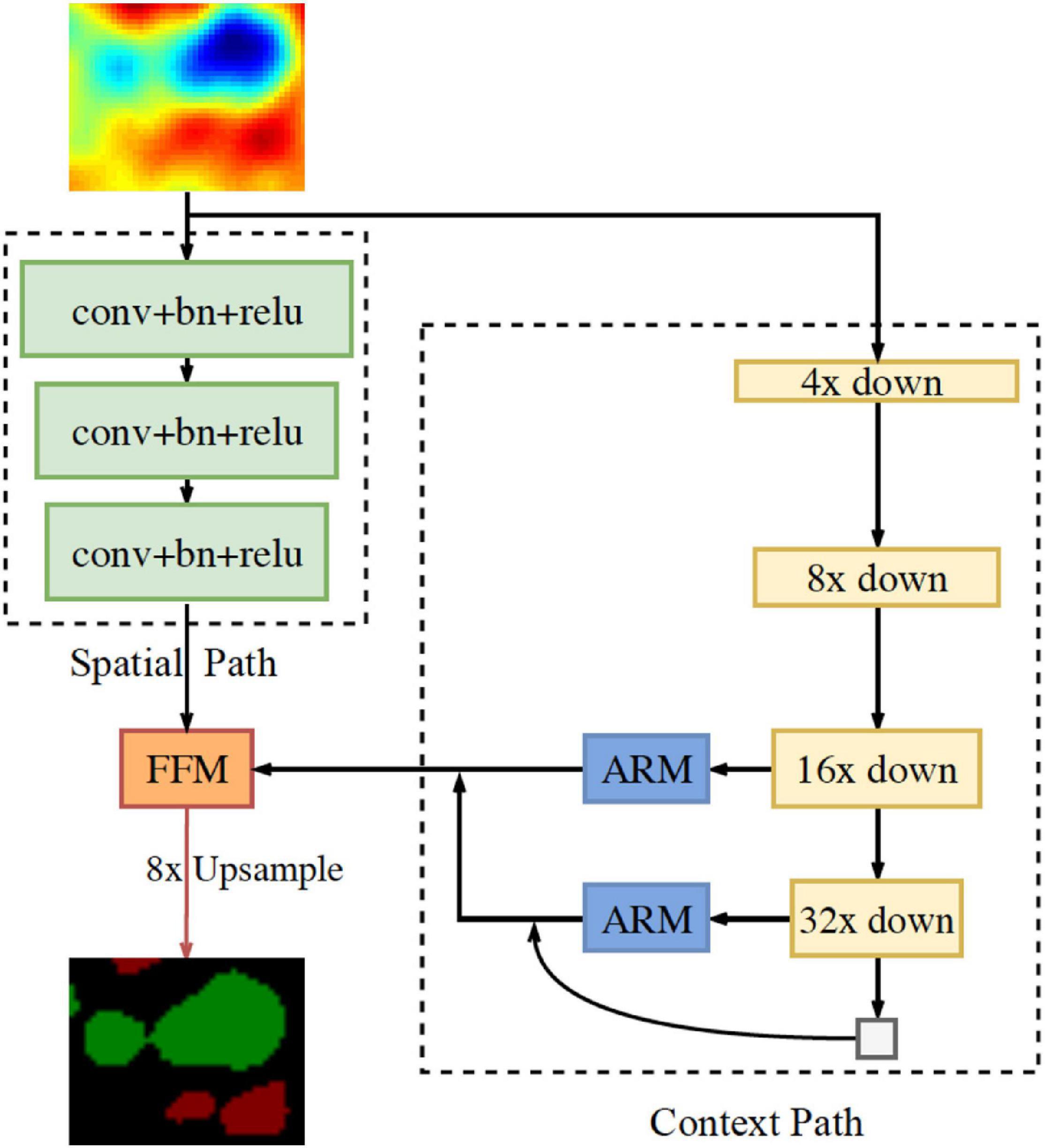
Figure 3. Schematic diagram of BiSeNet.

Vector Geometry—Based Eddy Detection Algorithm (VG)

We apply the method based on the geometry of velocity vectors of the flow field (Dong et al., 2009; Nencioli et al., 2010) for mesoscale eddy identification and tracking from geostrophic current, which is obtained from SSHA data. Eddy centers are determined by four criterions as follows (Nencioli et al., 2010): (a) along an east-west section, meridional velocity v has to reverse in sign across the eddy center and its magnitude has to increase away from it; (b) along a north—south section, zonal velocity u has to reverse in sign across the eddy center and its magnitude has to increase away from it: the sense of rotation has to be the same as for v; (c) velocity magnitude has a local minimum at the eddy center; and (d) around the eddy center, the directions of the velocity vectors have to change with a constant sense of rotation and the directions of two neighboring velocity vectors have to lay within the same or two adjacent quadrants. Eddy boundary is determined by the closed contour of the stream function field. Eddy tracks are retrieved by comparing the distribution of eddy centers at successive time steps. The tracking methods for the AI-based algorithms are the same as that for VG. The tracking method is one part of the VG, which can be found in Nencioli et al. (2010).

Data

Eddies were identified from daily SSHA data with a spatial resolution of 1/4° × 1/4°. The data, obtained from Copernicus Marine Environment Monitoring Service (CMEMS)¹, was a global product from multiple satellite altimeter along-track data. The SSHA data in the period from 2011 to 2015 were used in this study. The SSHA data were linearly interpolated onto a 1/8 × 1/8° grid to extend the eddy field for a larger number of grid points in order to improve further the performance of the eddy detection scheme (Liu et al., 2012). The SSHA data from 2011 to 2014 was used as the training data containing the labels of eddy information, while the 2015 were used as the validation set. This study focused on the North Pacific Subtropical Countercurrent (STCC, 15° N ∼ 30° N, 115° E ∼ 150° W), extending from east of Luzon Strait to the Hawaii Islands.

Results

The training SSHA data from 2011 to 2014 in the STCC region, which is labeled with cyclonic and anticyclonic eddies, is produced based on the traditional VG algorithm. In order to ensure validity and consistency of the training dataset, the eddy information are cleaned, dealing with invalid and missing data. Finally, the three different AI schemes are employed for deep learning with the training dataset from 2011 to 2014 and for eddy identification with the validation dataset during 2015.

The eddies identified based on the three different algorithms in the STCC region are compared on 19 August (Figure 4). Using the traditional VG algorithm, 172 ocean eddies are detected, including 84 cyclonic and 88 anticyclonic eddies. However, the other three deep learning algorithms all identify more eddies: 185 eddies (87 cyclonic and 98 anticyclonic eddies) from the PSPNet algorithm, 184 eddies (87 cyclonic and 97 anticyclonic eddies) from the DeepLabV3+ algorithm and 188 eddies (89 cyclonic and 99 anticyclonic eddies) from the BiSeNet algorithm.

FIGURE 4

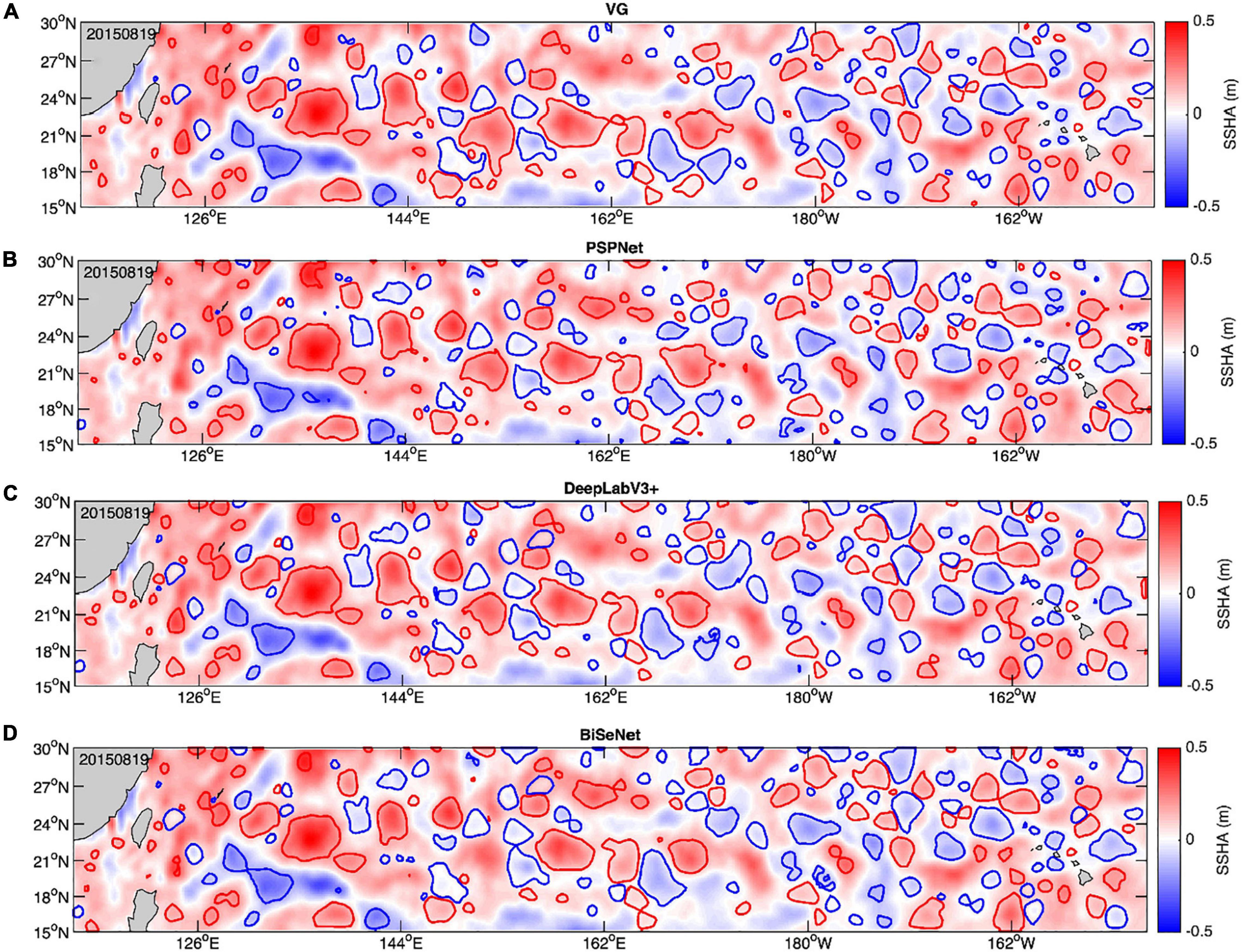
Figure 4. Oceanic eddies identified by VG (A), PSPNet (B), DeepLabV3+ (C), and BiSeNet (D) algorithms in the STCC region on 19 August 2015.

The comparisons of oceanic eddies detected from the AI-based algorithms are made based on a few eddy parameters, such as eddy number, size and lifetime.

Figure 5 compares the daily number of eddies detected by the VG, PSPNet, DeepLabV3+ and BiSeNet algorithms in the STCC region during 2015. A total of 68,010 oceanic eddies are identified by the VG algorithm, including 32,783 cyclonic and 35,227 anticyclonic eddies, which are less than those identified by the three AI algorithms. Among the three AI methods, the PSPNet algorithm detects the largest number of oceanic eddies (a total of 77,462 eddies). The DeepLabV3+ and the BiSeNet algorithm identify 72,264 and 75,579 eddies, respectively.

FIGURE 5

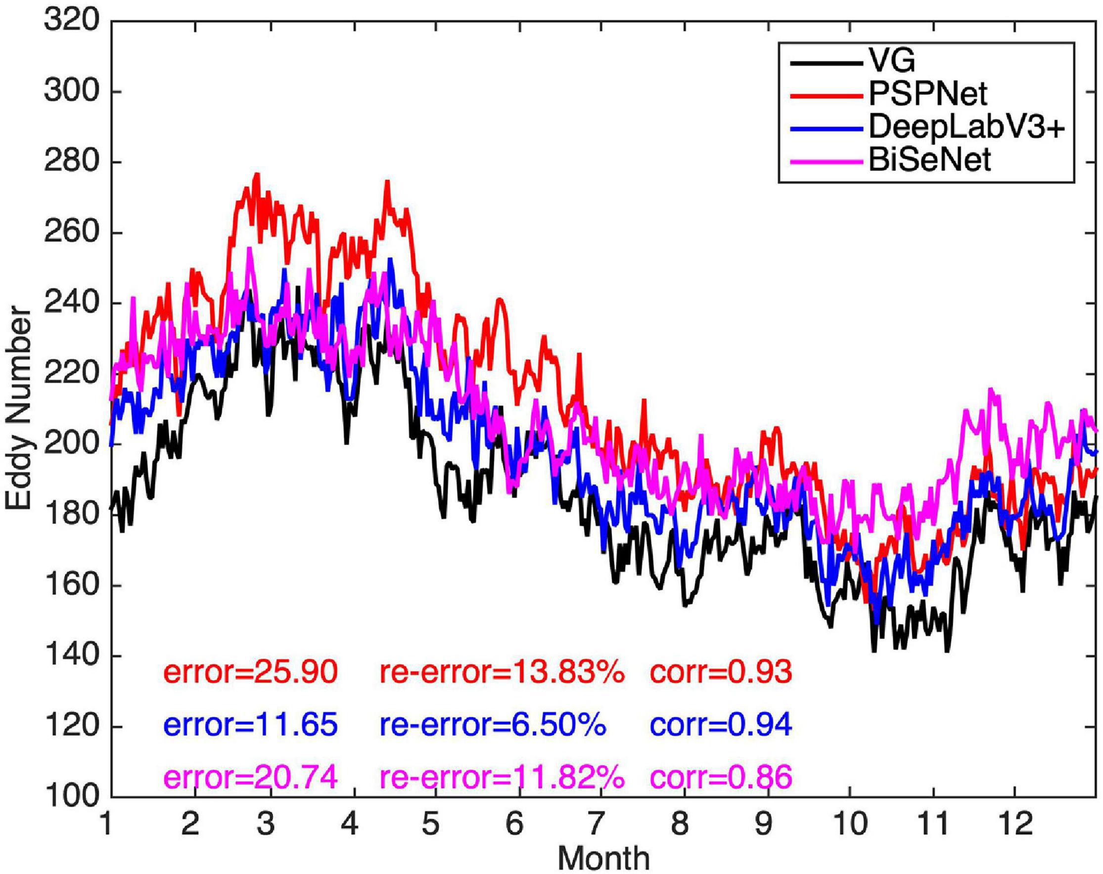
Figure 5. Time series of the daily number of eddies identified by the VG and three AI algorithms in the STCC region during 2015. Black, red, blue, and purple curves represent the results from VG, PSPNet, DeepLabV3+, and BiSeNer algorithm, respectively. “Error” is the difference between the three AI-based results and the VG results, “re-error” is the relative error which is defined as the error divided by the VG results, and “corr” is the correlation coefficient between the results from the three AI-based algorithms and the VG algorithm.

Compared with the traditional VG method results, the PSPNet, DeepLabV3+ and BiSeNet algorithm on average identify 25.90, 11.65, and 20.74 more eddies per day, respectively. There is a good correlation between the daily eddy numbers from the VG algorithm and the PSPNet (0.93), and the DeepLabV3+ (0.94) algorithm. The correlation of the daily eddy numbers between the BiSeNet and the VG method is less than the other two AI methods, with a correlation coefficient of 0.86. In Figure 6, the time series of the daily number of eddies detected by the DeepLabV3+ algorithm is the most consistent with that by the VG algorithm. In addition, based on the VG algorithm results, the differences in the results from the PSPNet and BiSeNet algorithms have seasonal variation characteristics. The PSPNet algorithm detected more eddies in spring and summer, while the BiSeNet algorithm detected a larger number of eddies in winter.

FIGURE 6

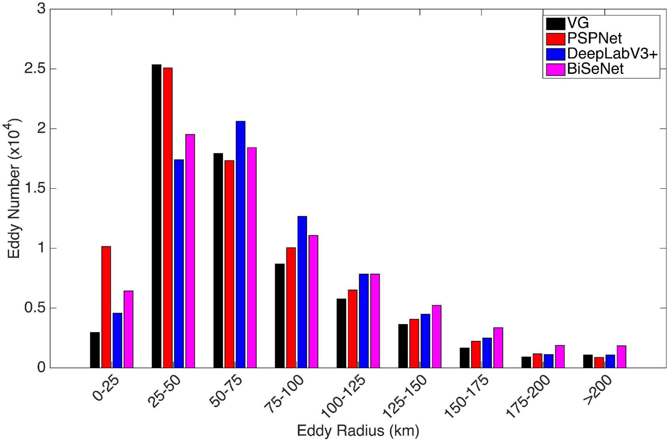
Figure 6. Size distribution of the identified eddies from the four different algorithms in the STCC region during 2015. Black, red, blue, and purple bars represent the results from VG, PSPNet, DeepLabV3+, and BiSeNet algorithm, respectively.

The radii of the oceanic eddies detected by the four different methods are compared in Figure 6. All the identified eddies peak at the 25–50 km bin, except for the DeepLabV3+, which has the highest number at the 50–75 km bin. The PSPNet algorithm has an obvious advantage in detecting small-scale eddies with radii of less than 25 km. The DeepLabV3+ algorithm identified the highest number of eddies with radius between 50 and 100 km. Furthermore, the BiSeNet algorithm detects more bigger eddies (greater than 100 km) than the other three methods.

The resolution of the altimetry data limits the presentation of small eddies. The facticity of the small-scale eddy needs further confirmation, so the results of detected eddies with radii less than 25 km are removed and the comparison among the algorithms is plotted in Figure 7. 64586 eddies are afterward detected by the VG method, while 65,034, 66,023, and 69,153 eddies are, respectively, detected by the PSPNet, DeepLabV3+ and BiSeNet algorithms. The differences between the traditional and AI-based results decrease with a similar pattern during 2015. The BiSeNet algorithm identifies the largest number of oceanic eddies among the three AI-based methods. 12.51 eddies more, on average, are identified per day with a relative error of 7.74%. It is suggested that the BiSeNet algorithm takes an advantage in identifying large-scale eddies, which can be verified in Figure 6. However, the majority of the additional eddies detected by the PSPNet algorithm are small-scale ones.

FIGURE 7

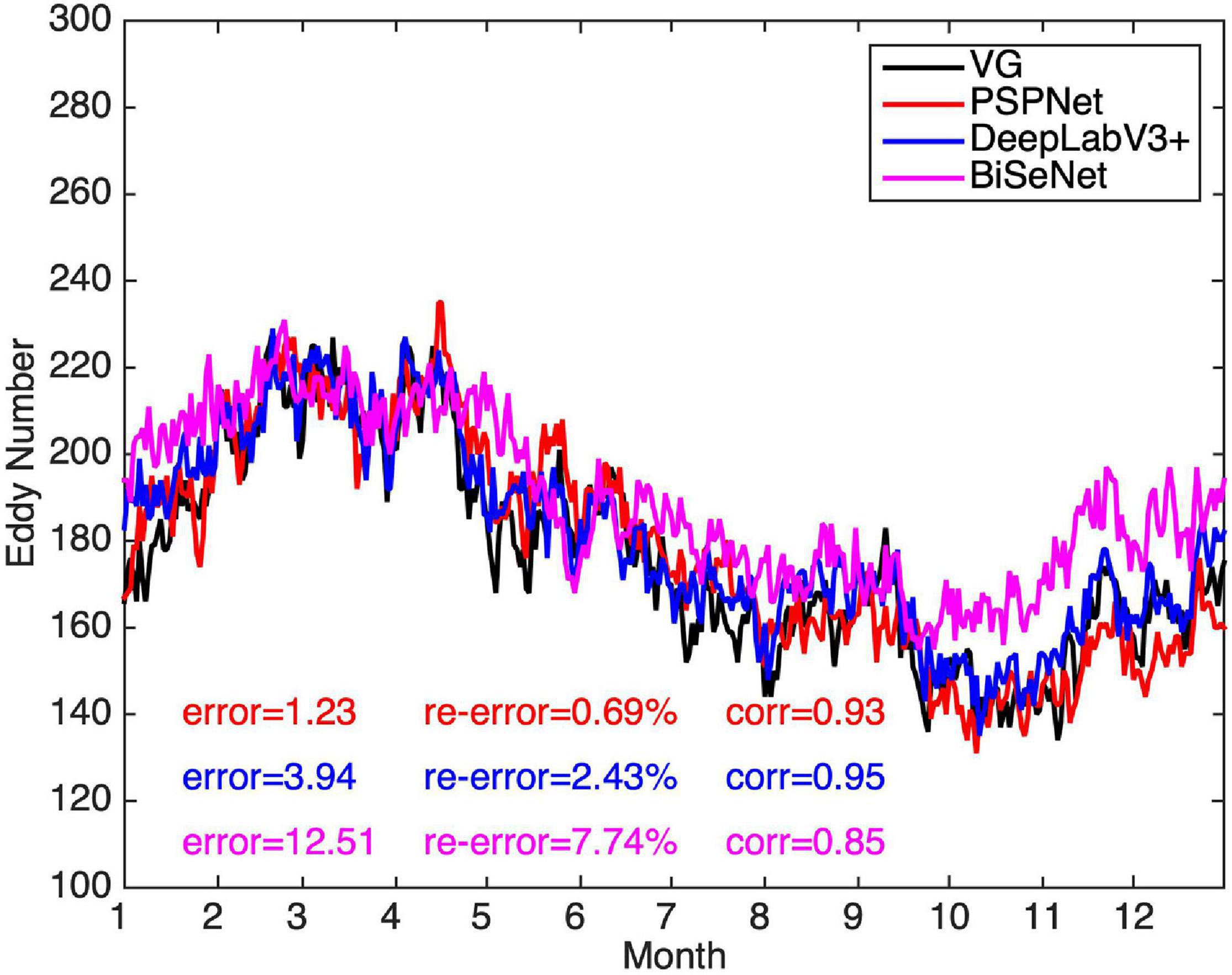
Figure 7. Same as Figure 5 except for the comparison of the daily number of eddies with radii greater than 25 km.

Lifetime is another important eddy characteristic. The lifetime distribution of the eddies identified by the four algorithms are presented in Figure 8. A total of 844 eddies with lifetimes greater than 4 weeks (387 anticyclones and 457 cyclones) are identified by the traditional VG algorithm. Considering eddies which survive more than 4 weeks, the PSPNet, DeepLabV3 + and BiSeNet algorithms detect 875 eddies (400 anticyclonic and 475 cyclonic eddies), 805 eddies (370 anticyclonic and 435 cyclonic eddies), and 819 eddies (383 anticyclonic and 436 cyclonic eddies), respectively. The eddies identified by the three AI algorithms survive longer than that identified by the VG algorithm because the AI algorithms can detect small-sized eddies during the growing and decaying periods. Among the three AI-based methods, eddies detected by the DeepLabV3+ algorithm have the shortest lifetimes.

FIGURE 8

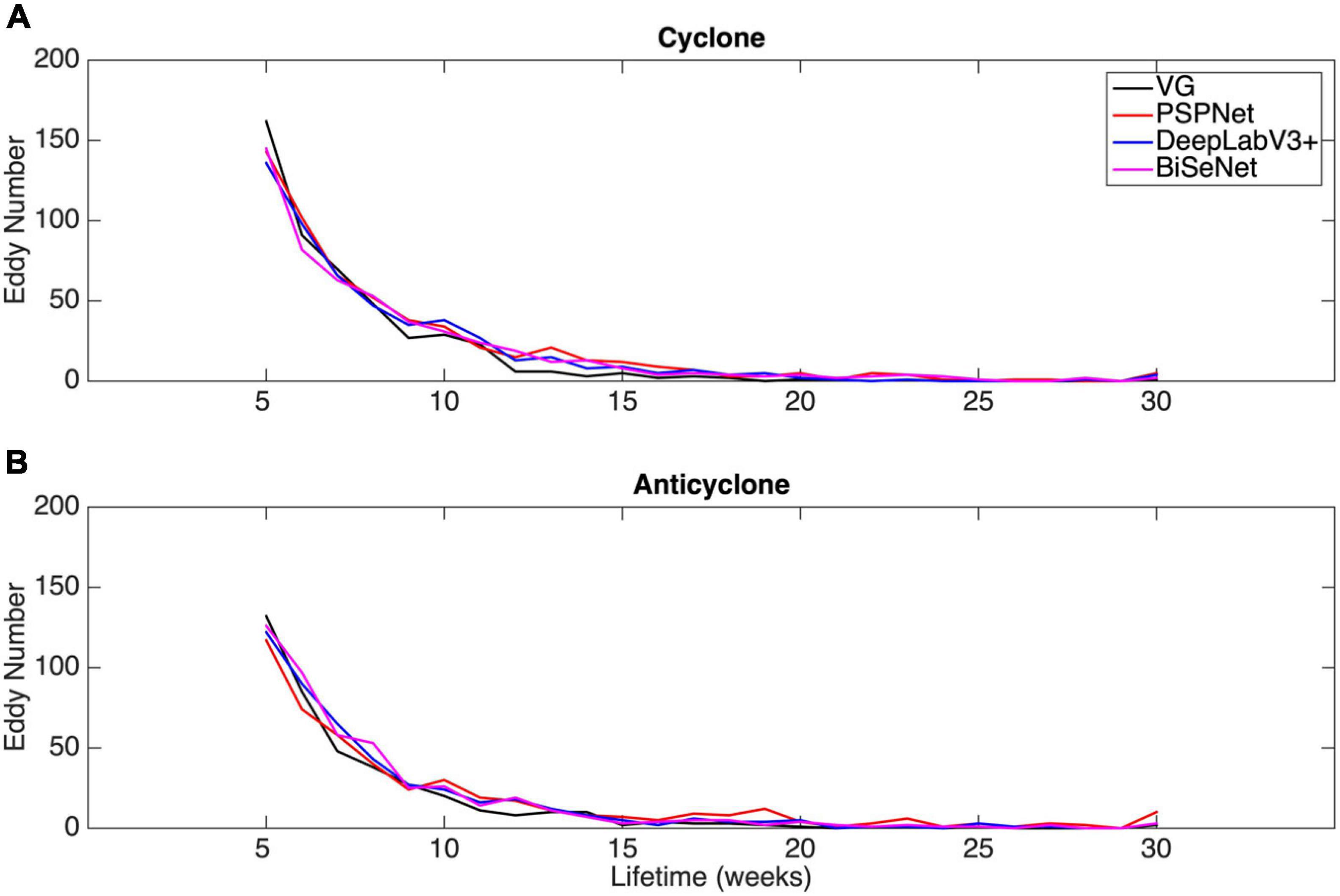
Figure 8. Lifetime distribution of eddies identified by the VG (black), PSPNet (red), DeepLabV3+ (blue), and BiSeNet (purple) algorithms in the STCC region during 2015. (A) Cyclones; (B) anticyclones.

Discussion

In order to further discuss the AI-based results, the eddies identified by the AI-based algorithms and by the VG algorithm in the STCC region during 2015 are compared with mesoscale eddy trajectory atlas product (Ver 2.0), which is obtained from AVISO+². Since the AVISO+ product provides the eddies with the lifetimes longer than 4 weeks but without the boundary information (only radius), only the center locations of the eddies with the lifetimes longer than 4 weeks and with the radii greater than 25 km in the STCC region on June 07, 2015 are plotted in Figure 9 for the comparison of the results from the five versions. The PSPNet algorithm detects the most oceanic eddies (176 eddies) of the three versions, followed by 142 ones for the AVISO+ version, 137 ones for the VG version, 128 ones for the BiSeNet version and 125 ones for the DeepLabV3+. During the 1 year period, 637 eddy tracks are totally obtained from the AVISO product, all of which survive longer than 4 weeks. The PSPNet algorithm detects 875 eddy tracks with lifetimes longer than 4 weeks, while 844 tracks by the VG algorithm, 819 tracks by the BiSeNet and 805 tracks by the DeepLabV3+. The number of eddy tracks from the AVISO+ version is the smallest among those from the five versions.

FIGURE 9

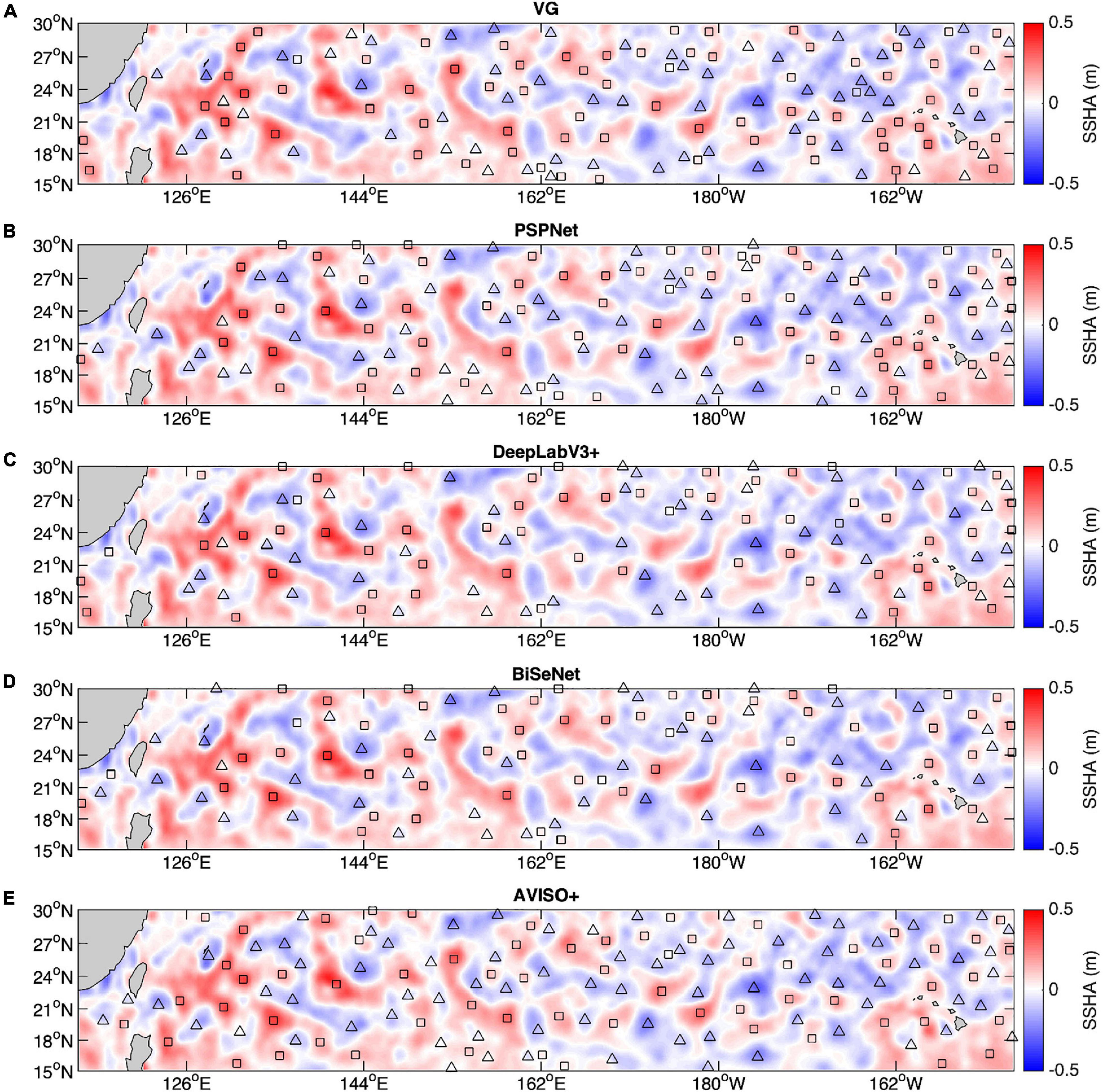
Figure 9. Comparison of the oceanic eddies longer than 4 weeks from the five versions in the STCC region on June 07, 2015. (A) The VG version; (B) the PSPNet version; (C) the DeepLabV3+ version; (D) the BiSeNet version; (E) the AVISO+ version. Triangles and squares represent the center of the cyclonic and anticyclonic eddies, respectively.

Several eddy parameters are compared among these five results in Table 1. The mean lifetimes of eddies identified by the AI-based algorithms are all shorter than that from the AVISO+ version but longer than that detected by the VG algorithm. The eddies from the AVISO+ version, the PSPNet version and the BiSeNet version survive for up to a year. The mean amplitude (9.3 cm) and the mean radius (104.6 km) of the eddies from the BiSeNet version are greater than those from the other four versions, which suggests that the BiSeNet has an advantage in large-scale eddy. And the maximum eddy radii are all larger than 260 km, even close to 300 km, for the five versions. The mean displacements of the eddies from the AI-based versions and the VG version are both shorter than that from the AVISO+ version. But the eddies from the PSPNet version and the AVISO+ version moves up to more than 3,000 km. Furthermore, the eddies from the three versions propagate with the similar mean speed at 6.3 ∼7.8 km day^–1.

TABLE 1

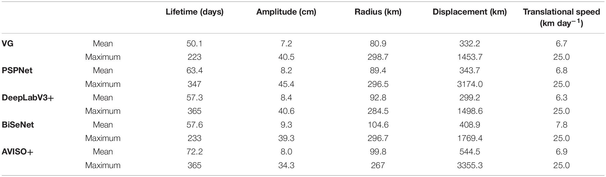
Table 1. Comparisons of eddy properties base on the five results.

Conclusion

Compared to the traditional eddy detection method, deep learning-based algorithms are novel. Three different AI-based algorithms were applied to identify ocean eddies, including the PSPNet, DeepLabV3+ and BiSeNet algorithms. SSHA data from 2011 to 2014 in the STCC region, labeled with eddy information detected by the VG algorithm, are employed for training, and SSHA data in 2015 used for validation. Eddies detected by the three AI-based methods are compared with each other and with the results from the traditional method. All three AI-based algorithms extract more eddies than the traditional VG algorithm. The PSPNet algorithm detects the highest number of eddies. The BiSeNet algorithm performs better in large-scale eddy identification than the other two AI-based algorithms, because the Spatial Path is introduced into the algorithm to avoid destroying the eddy edge information. The eddies identified by the AI-based algorithms tend to survive longer than those identified by the VG method. The lifetimes of the eddies extracted by the DeepLabV3+ algorithm are the shortest among the results from the AI-based methods.

Data Availability Statement

The original contributions presented in the study are included in the article/supplementary material, further inquiries can be directed to the corresponding author/s.

Author Contributions

GX and CD contributed to the designing and planning the experiments and writing the manuscript. WX and XG performed the experiments and revised the manuscript. All authors contributed to the article and approved the submitted version.

Funding

This study was supported by the project supported by Southern Marine Science and Engineering Guangdong Laboratory (Zhuhai) (SML2020SP007), the Guangdong Basic and Applied Basic Research Foundation (2019A1515110840), the Key Program of Marine Economy Development (Six Marine Industries) Special Foundation of Department of Natural Resources of Guangdong Province [GDNRC(2020)049], the National Natural Science Foundation of China (42076162), the Natural Science Foundation of Guangdong Province of China (2020A1515010496), and the Research Startup Foundation of Guangdong Ocean University (R20009).

Conflict of Interest

The authors declare that the research was conducted in the absence of any commercial or financial relationships that could be construed as a potential conflict of interest.

Acknowledgments

The authors would like to thank AVISO+ for providing SSHA data and mesoscale eddy trajectory atlas product. The authors would like to thank GitHub for providing AI programs. The authors would also like to thank Zhoutong Technology ILC (UNIVER) for their competent comments and technical guidance.

Footnotes

1. ^ http://marine.copernicus.eu
2. ^ https://www.aviso.altimetry.fr/en/data/products/value-added-products/global-mesoscale-eddy-trajectory-product.html

References

Chaigneau, A., Gizolme, A., and Grados, C. (2008). Mesoscale eddies off peru in altimeter records: identification algorithms and eddy spatio-temporal patterns. Prog. Oceanogr. 79, 106–119. doi: 10.1016/j.pocean.2008.10.013

CrossRef Full Text | Google Scholar

Chelton, D. B., Schlax, M. G., Samelson, R. M., and De Szoeke, R. A. (2007). Global observations of large oceanic eddies. Geophys. Res. Lett. 34:L15606. doi: 10.1029/2007GL030812

CrossRef Full Text | Google Scholar

Chen, L. C., Papandreou, G., Kokkinos, I., Murphy, K., and Yuille, A. L. (2016). Image segmentation with deep convolutional fully connected CRFs. arXiv[Preprint]. Available online at: https://arxiv.org/abs/1412.7062 (accessed March 23, 2019).

Google Scholar

Chen, L. C., Papandreou, G., Schroff, F., and Adam, H. (2017). Rethinking atrous convolution for semantic image segmentation. arXiv[Preprint]. Available online at: https://arxiv.org/abs/1706.05587 (accessed March 23, 2019).

Google Scholar

Dong, C., Liu, Y., Lumpkin, R., Lankhorst, M., Chen, D., Mcwilliams, J. C., et al. (2011a). A scheme to identify loops from trajectories of oceanic surface drifters: an application in the Kuroshio Extension Region. J. Atmos. Ocean. Tech. 28, 1167–1176. doi: 10.1175/JTECH-D-10-05028.1

CrossRef Full Text | Google Scholar

Dong, C., Mavor, T., Nencioli, F., Jiang, S., Uchiyama, Y., Mcwilliams, J. C., et al. (2009). An oceanic cyclonic eddy on the lee side of Lanai Island, Hawai’i. J. Geophys. Res. 114:C10008. doi: 10.1029/2009JC005346

CrossRef Full Text | Google Scholar

Dong, C., McWilliams, J. C., Liu, Y., and Chen, D. (2014). Global heat and salt transports by eddy movement. Nat. Commun. 5:3294. doi: 10.1038/ncomms4294

PubMed Abstract | CrossRef Full Text | Google Scholar

Dong, C., Nencioli, F., Liu, Y., and McWilliams, J. C. (2011b). An automated approach to detect oceanic eddies from satellite remotely sensed sea surface temperature data. IEEE Geosci. Remote Sens. 8, 1055–1059. doi: 10.1109/LGRS.2011.2155029

CrossRef Full Text | Google Scholar

Du, Y., Song, W., He, Q., Huang, D., Liotta, A., and Su, C. (2019). Deep learning with multi-scale feature fusion in remote sensing for automatic oceanic eddy detection. Inform. Fusion 49, 89–99. doi: 10.1016/j.inffus.2018.09.006

CrossRef Full Text | Google Scholar

Duo, Z., Wang, W., and Wang, H. (2019). Oceanic mesoscale eddy detection method based on deep learning. Remote Sens. 11:1921. doi: 10.3390/rs11161921

CrossRef Full Text | Google Scholar

Faghmous, J. H., Chamber, Y., Boriah, S., Liess, S., and Mesquita, S. (2012). “A novel and scalable spatio-temporal technique for ocean eddy monitoring,” in Proceedings of the Twenty-Sixth AAAI Conference on Artificial Intelligence, (Menlo Park, CA: AAAI).

Google Scholar

Franz, K., Roscher, R., Milioto, A., Wenzel, S., and Kusche, J. (2018). “Ocean eddy identification and tracking using neural networks,” in Proceedings of the International Geoscience and Remote Sensing Symposium 2018, (Valencia).

Google Scholar

He, K., Zhang, X., Ren, S., and Sun, J. (2014). Spatial pyramid pooling in deep convolutional networks for visual recognition. IEEE Trans. Pattern Anal. Mach. Intell. 37, 1904–1916.

Google Scholar

Lguensat, R., Sun, M., Fablet, R., Mason, E., Tandeo, P., and Chen, G. (2017). EddyNet: a deep neural network for pixel-wise classification of oceanic eddies. arXiv[Preprint]. doi: 10.1109/IGARSS.2018.8518411

CrossRef Full Text | Google Scholar

Liu, Y., Dong, C., Guan, Y., Chen, D., McWilliams, J., and Nencioli, F. (2012). Eddy analysis in the subtropical zonal band of the North Pacific Ocean. Deep Sea Res. 1 Oceanogr. Res. Pap. 68, 54–67. doi: 10.1016/j.dsr.2012.06.001

CrossRef Full Text | Google Scholar

Moreau, S., Penna, A. D., Llort, J., Patel, R., Langlais, C., Boyd, P. W., et al. (2017). Eddy-induced carbon transport across the Antarctic Circumpolar Current. Glob. Biogeochem. Cycles 31, 1368–1386. doi: 10.1002/2017GB005669

CrossRef Full Text | Google Scholar

Nencioli, F., Dong, C., Dickey, T., Washburn, L., and McWilliams, J. C. (2010). A vector geometry-based eddy detection algorithm and its application to a high-resolution numerical model product and high-frequency radar surface velocities in the Southern California Bight. J. Atmos. Ocean. Tech. 27, 564–579. doi: 10.1175/2009JTECHO725.1

CrossRef Full Text | Google Scholar

Patel, R. S., Llort, J., Strutton, P. G., Phillips, H. E., Moreau, S., Pardo, P. C., et al. (2020). The biogeochemical structure of Southern Ocean mesoscale eddies. J. Geophys. Res. Oceans 125:e2020JC016115. doi: 10.1029/2020JC016115

CrossRef Full Text | Google Scholar

Patel, R. S., Phillips, H. E., Strutton, P. G., Lenton, A., and Llort, J. (2019). Meridional heat and salt transport across the subantarctic front by cold-core eddies. J. Geophys. Res. Oceans 124, 981–1004. doi: 10.1029/2018JC014655

CrossRef Full Text | Google Scholar

Xu, G., Cheng, C., Yang, W., Xie, W., Kong, L., Hang, R., et al. (2019). Oceanic eddy identification using an AI scheme. Remote Sens. 11:1349. doi: 10.3390/rs11111349

CrossRef Full Text | Google Scholar

Yu, C., Wang, J., Peng, C., Gao, C., Yu, G., and Sang, N. (2018). Bisenet: Bilateral Segmentation Network for Real-Time Semantic Segmentation. arXiv[Preprint]. Available online at: https://arxiv.org/abs/1808.00897 (accessed May 15, 2019).

Google Scholar

Yu, F., and Koltun, V. (2016). Multi-Scale Context Aggregation by Dilated Convolutions. arXiv[Preprint]. Available online at: https://arxiv.org/abs/1511.07122 (accessed May 15, 2019).

Google Scholar

Zhao, H., Shi, J., Qi, X., Wang, X., and Jia, J. (2017). “Pyramid scene parsing network,” in Proceedings of the 2017 IEEE Conference on Computer Vision and Pattern Recognition (CVPR), (Geneva).

Google Scholar