A Glider Simulation Model Based on Optimized Support Vector Regression for Efficient Coordinated Observation

Multi-gliders have been widely deployed as an array in nowadays ocean observation for fine and long-term ocean research, especially in deep-sea exploration. However, the strong, variable ocean currents and the delayed information feedback of gliders are remaining huge challenges for the deployment of glider arrays which may cause that the observed data cannot meet the study needs and bring a prohibitive cost. In this paper, we develop a Glider Simulation Model (GSM) based on the support vector regression with the particle swarm optimization (PSO)-SVR algorithm to integrate the information feedback from gliders and ocean current data for rapid modeling to effectively predict the gliders’ trajectories. Based on the real-time predictive information of the trajectories, each glider can select future movement strategies. We utilize the in-suit datasets obtained by sea-wing gliders in ocean observation to train and test the simulation model. The results show that GSM has an effective and stable performance. The information obtained from the modeling approaches can be utilized for the optimization of the deployment of the glider arrays.

Introduction

Underwater gliders are characterized as a type of persistent (can operate continuously for weeks to months even to years), long operation range (up to thousand kilometers), small power consumption, and unmanned marine vehicle which are propelled by buoyancy (Rudnick et al., 2004). These characteristics make them conduct long-term ocean studies and understand the inner working mechanisms of the ocean in a controllable way which are better than existing traditional instruments for ocean observation (Testor et al., 2019). In recent years, with the widespread attention aroused by researchers on ocean observation, especially on deep ocean, gliders are widely deployed in ocean studies (Liblik et al., 2016).

Furthermore, in the major ocean observation, multiple gliders are deployed as a glider array to develop surveys to optimize and refine the ocean sampling. Shu et al. (2019) deploy 12 gliders as an observation network in the northern South China Sea (NSCS) for the research on anticyclonic eddies. The observations reveal not only the fine subsurface structure of temperature and salinity but also the time evolution of the three-dimensional structure of the eddies. Li et al. (2019) not only equip the glider observation array with CTDs to reveal the three-dimensional structure of the anticyclonic eddies in NSCS but also mount the biogeochemical sensors on the gliders which can show the influence of anticyclonic eddies on the biogeochemical structure. On this basis, a compound three-dimensional structure of the eddy is constructed.

Although glider arrays present a compelling advantage in ocean observation, there are challenging difficulties on deployment. The movements of gliders are closely related to dynamic ocean currents (Thompson et al., 2010); the high nonlinearity of disturbances may make the actual observation trajectories of gliders not consistent with the planned running trajectories, which can cause the redundant measurement or the incomplete measurement during the experiments (Zhang et al., 2007). Meanwhile, the position information of gliders will only be transmitted when the gliders come out of the water; the asynchrony of information synchronization prevents the accuracy of the simulation on the trajectory control of glider arrays. Furthermore, conducting a coordinated observation with multiple gliders in large-scale ocean experiments is expensive.

Several prior studies have focused on these problems. Rao and Williams (2009) considered the influence of ocean currents and proposed a path planning method based on rapidly exploring random trees (RRT). However, this path planning method is based on the assumption that we have accurate knowledge of future currents, which is nondeterministic in practice. Thompson et al. (2010) presented a method with historical ocean current predictions to address the glider path planning and control in the uncertain, time-varying ocean currents. Besides, to solve the problem that currents may drive glider arrays into clumps without feedback information (Leonard et al., 2007). Paley et al. (2008) designed a control system named Glider Coordinated Control System (GCCS) which, through the real-time feedback control law, coordinates the gliders and optimizes the glider measurement formations. The study of Leonard et al. (2010) confirmed the capacity of the GCCS applied to ocean sampling. Considering avoiding the collisions between gliders, a navigation system based on Networked Decentralized Model Predictive Control was developed to coordinate the gliders into the desirable formation (Fonti et al., 2011). This method has high autonomy and reliability but only considers the horizontal plane motion. Xiong et al. (2020) discussed a rapidly exploring random tree star (RRT^∗) method which is a variant algorithm of standard RRT to meet the need of collision avoidance and achieve continuous sampling effectively. Xue et al. (2018) also proposed a strategy of the control of hybrid gliders that merge the coordinate control model based on artificial potential fields with a motion optimization method. In a recent study, Clark et al. (2020) decoupled a vehicle motion model with a predictive ocean current model forming an adaptive planner that glider observation arrays can maintain stability.

However, most of the studies are pointing at the nonlinear mechanical model of the underwater glider and the uncertain ocean current predictive model, as the actual conditions of gliders and ocean currents can quickly diverge in practice and the existing studies are not feasible to reconfigure the glider arrays according to actual conditions in different sea states. Thus, in this paper, we design a glider simulation model (GSM), considering multiple factors, which can rapidly feedback information from gliders and provide real-time predictive information of coordination of gliders. Based on the predictive information, each glider can determine future motion strategies. In this model, we introduce support vector regression based on PSO-SVR as the supporting algorithm. Although the information feedback from gliders contains non-inear fluctuations, noise, and outliers, the PSO-SVR algorithm can well grasp the movement trend. As far as we know, few studies have employed PSO-SVR to optimize glider control and formation deployment. We also introduce three observation datasets obtained by sea-wing gliders into the simulation experiments; the results demonstrate that the GSM has great stability and effectiveness on sea-wing gliders.

The rest of the paper is made up as follows: the summary of the dataset is shown in section “Data.” In section “Methods,” we give a comprehensive introduction to the methods involved in the model. Section “Experiments” presents the results of the experiments using different algorithms, and a full comparison of the performance is evaluated. In the last section, we draw the conclusion and increase the future works needed to be done to improve our simulation model.

Data

Glider Data

Sea-wing gliders are selected to verify the validity of the model (Figure 1C). Three sets of in-suit observation data collected by sea-wing gliders are employed to train and test the simulation model. These datasets come from two ocean observation experiments where the investigation areas are located in the northern South China Sea.

FIGURE 1

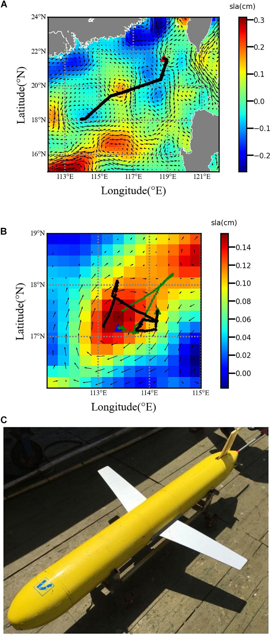
Figure 1. The trajectories of gliders in the ocean observation. (A) The observation started from April 28, 2015 to June 1, 2016. (B) The observation started from July 3, 2016 to July 16, 2016. The triangles indicate the starting points of observations. The backgrounds are the sea-level anomaly in the observation areas, and the arrows indicate the ocean current field. (C) Picture of the sea-wing glider.

G-001 dataset: The experiment started from April 28, 2015, to June 1, 2015, employing one glider (g-001) for the cross-sectional observation of eddies, and the trajectory of the glider is shown in Figure 1A.

G-002 dataset: The experiment started from July 3, 2016, to July 16, 2016, and lasted for 17 days. During the experiment, a sea-wing glider (g-002) with multiple sensors is deployed for the inner observation of eddies, and the trajectory is shown in Figure 1B; the black line represents the trajectory of g-002.

G-003 dataset: The experiment started from July 3, 2016, to July 16, 2016, with a sea-wing glider (g-003) carrying one sensor for cross-eddy observation. We can see the trajectory in Figure 1B; the green line is the trajectory of g-003.

The triangles indicate the starting points of observations. The backgrounds are the sea-level anomaly in the observation areas where the higher the anomaly, the greater the possibility of the existence of eddies. The arrows indicate the ocean current field, and the size of arrows represents the strength of the geostrophic currents.

AVISO Ocean Current Dataset

The ocean current dataset used in this study was distributed by AVISO and derived from the absolute dynamic topography (ADT), which can be downloaded from the website¹.

Methods

In this section, we present an overview of the method that we adopt to train and test the simulation model.

SVR for Data Regression

SVR is an extended algorithm of the support vector machine (SVM) which is a classic and powerful machine-learning algorithm to solve the nonlinear regression problem (Brereton and Lloyd, 2010). SVR calculates the loss function based on the structural risk minimization, allowing a deviation of ε between the output of the model and the real value, which differs from the traditional regression model based on the error between the output of the model and the real output. It can avoid the disadvantages caused by pursuing experience risk minimization.

In this subsection, we concisely describe the basic theory of the SVR algorithm. We can learn more detailed theories from Smola and Scholkopf (2004). In our study, the whole diving and climbing process of the glider is described as the dataset S ={(x_i,y_i)}. x_i = {P_i,D_i,V_i} denotes the parameters of the ith diving process. P_i denotes the position in which the glider dives into the water which is observed by the GPS equipped on the glider. D_i is the target diving depth, and V_i represents the velocity at the diving point from the AVISO. y_i represents the real GPS coordinate of the point that the glider comes out of the water during the ith climbing process. The objective of the algorithm is to build a regression model to predict the location that the glider comes out of the water in the following form:

$$\begin{array}{c}\hfill f\left(x_i\right)=w^T{x}_i+b,\hfill \\ \hfill y_i-w^T{x}_i-b\le \mathrm{\epsilon },\hfill \\ \hfill w^T{x}_i+b-y_i\le \mathrm{\epsilon },\hfill \\ \hfill \mathrm{\epsilon }\ge 0\hfill \end{array}(1)$$

where w and b are, respectively, the slope and offset coefficient generated in the process of mapping x_i to f(x_i), which is optimized during the training of the model. f(x_i) is the predicted location that the glider comes out of the water, whileε denotes the deviation between f(x_i) and y_i. The loss is calculated when the error between the predicted value and the real value is greater than ε. So, the regression problem can be formalized as minimizing the convex optimization problem as follows:

$$min\frac{1}{2}{||w||}^2+C\sum _{i=1}^m\mathrm{\beth }\left(f\left(x_i\right)-y_i\right)(2)$$

In this equation, C is the regularization parameter, and ℶ is the ε –insensitivate loss function to assess the accuracy of the model. Generally speaking, it is difficult to define the appropriate ε to ensure that f(x), all pairs (x_i,y_i), and the slack variables ξ_i and ${\xi }_i^{*}$ are introduced. The regression problem can be reformulated as the following constraints:

$$\begin{array}{c}\hfill min\frac{1}{2}{||w||}^2+C\sum _{i=1}^m\left({\xi }_i+{\xi }_i^{*}\right),\hfill \\ \hfill s.t.y_i-w^T{x}_i-b\le \mathrm{\epsilon }+{\xi }_i,\hfill \\ \hfill w^T{x}_i+b-y_i\le \mathrm{\epsilon }+{\xi }_i^{*},\hfill \\ \hfill {\xi }_i,{\xi }_i^{*}\ge 0,i=1,2,\mathrm{\dots },N\hfill \end{array}(3)$$

By applying the Lagrange multiplier method and KKT condition, the problem can be expressed as the following equations:

$$\begin{array}{c}\hfill f\left(x\right)=\sum _{i=1}^m\left({\widehat{\mathrm{\alpha }}}_i-{\mathrm{\alpha }}_i\right)K(x_i^T,x_i)+b,\hfill \\ \hfill s.t.\sum _{i=1}^m\left({\widehat{\mathrm{\alpha }}}_i-{\mathrm{\alpha }}_i\right)=0,\hfill \\ \hfill \mathrm{\hspace{0.25em}0}\le {\mathrm{\alpha }}_i,{\widehat{\mathrm{\alpha }}}_i\le C\hfill \end{array}(4)$$

where α_i and ${\widehat{\mathrm{\alpha }}}_i$ are the Lagrange coefficients, and $K(x_i^T,x_i)$ is the kernel function. The Lagrange multiplier method can transform constrained inequalities into unconstrained equations, and the KKT condition can transform the nonlinear regression problem into an approximate linear regression problem. In our study, the kernel function named radial basis function (RBF) was mentioned which can project vectors into any dimensional space. The equation is described by:

$$\begin{array}{c}\hfill K(x_i,x_j)=exp\left(-\frac{{||x_i-x_j||}^2}{2{\mathrm{\sigma }}^2}\right),\hfill \\ \hfill \mathrm{\sigma }\ge 0\hfill \end{array}(5)$$

where x_i and x_j are the input vector space, and σ is the bandwidth of RBF.

From the above equations, we can see that two hyperparameters heavily affect the performance of the SVR, namely, the regularization parameter C which represents the tolerance for error and the bandwidth of RBF σ which determines the influence scope of each vector. The appropriate selection of these hyperparameters can significantly improve the performance of SVR. However, a trial-and-error approach to optimize hyperparameters needs much time and is not practical. In our study, we employ the PSO algorithm to optimize parameters.

PSO for Optimizing Parameters

Although SVR is a powerful algorithm for regression problems, its effectiveness is easily affected by the selection of hyperparameters (Kim et al., 2020). Inappropriate parameter selection can easily lead to over-fitting or under-fitting of the prediction results which can affect the coordination of glider arrays. In early studies of the SVR, the grid search method is widely adopted to tune hyperparameters (Jiang et al., 2013). In recent years, many heuristic algorithms have been used to optimize the hyperparameters.

PSO is a technology of evolutionary computing proposed by Kennedy and Eberhart (1995), which has advantages at accelerating the process of tuning the SVR parameters and getting the optimum. The main idea of the algorithm is to analogize the process of optimizing parameters as birds looking for food. Under the constraints of the fitness function, particles keep adjusting speed and position through collaboration and information sharing between each particle to find the final optimum solution.

The particle speed update equation is:

$$v_i=w\times v_i+c_1\times rand()\times \left(pbes{t}_i-x_i\right)+c_2\mathrm{}\times rand()\times (gbest-x_i)(6)$$

where i = 1,…,n ∈ Rⁿ denotes the number of particles, v_i represents the speed of the particle, pbest_i is the optimal parameter under current training steps, gbest indicates the global optimal parameter under current training steps, x_i is the particle position, rand() represents the random number between (0,1), w is the inertia factor which affects the capability of global optimization and local optimization of the algorithm, c₁ indicates the level that the particle updating is affected by the local optimal particle, and c₂ is the level that the particle updating is affected by the global optimal particle.

The particle position update equation is:

$$x_i=x_i+v_i(7)$$

In our study, to find the best hyperparameters (C,σ), the process is shown as follows:

First, we set PSO parameters, the number of particles is 30, the dimension is 2, the iteration steps are 50, and the space ranges of the solutions are from 0.1 to 5. Second, randomly generating the initial value of hyperparameters includes the prime velocities and the initial positions of the swarm of particles in search space. Third, we utilize the parameters in each particle to construct the SVR model and calculate the values of the fitness function, through the values of fitness function to update pbest_i and gbest. Last, if the experiment meets the iteration steps or the value of fitness function reaches the extent predefined, we stop updating and choose gbest as the best hyperparameters (C,σ); otherwise, we return to Third.

Experiments

In this section, we conduct experiments to evaluate the accuracy and efficiency of the simulation model. We use the glider datasets to train and test the simulation model where 75% of each dataset are employed as the training samples for the training and parameter optimization. The rest are applied as the testing samples. We also select several other algorithms as the baseline to compare them with our algorithm. The key idea of our experiment is to utilize the information feedback from gliders for rapid modeling to generate the trajectories of gliders and minimize the error between real trajectory and predicted trajectory.

Data Standardization

In this subsection, to eliminate adverse effects caused by singular sample data, we standardized the data before conducting experiments. The training data S ={(x_i,y_i)} are standardized in the normalization function of min–max normalization:

$$S_{train}=\frac{S-min(S)}{max\left(S\right)-min(S)}(8)$$

where S_train represents the standardized value.

The Experiment Results and Discussion

The Results of Parameter Optimization

In this subsection, we demonstrate the hyperparameters optimized by the PSO algorithm. The optimization of parameters uses an iterative approach, and the iterative results can be learned from Figure 2 where the x-axis represents the number of iteration steps, the y-axis represents the fitness values, the yellow lines indicate the fitness values in the longitudinal direction, and the blue lines represent the fitness values in the latitudinal direction. The process of optimization is the coordinated adjustment of particles to find the optimal fitness value. We can see that with the increase of iteration steps, the fitness values keep decreasing until achieving stability. The stability of fitness values means that all particles achieve an individual best fitness and the PSO-SVR model achieves the optimal hyperparameters (C,σ); we can learn the optimization results in Figure 2.

FIGURE 2

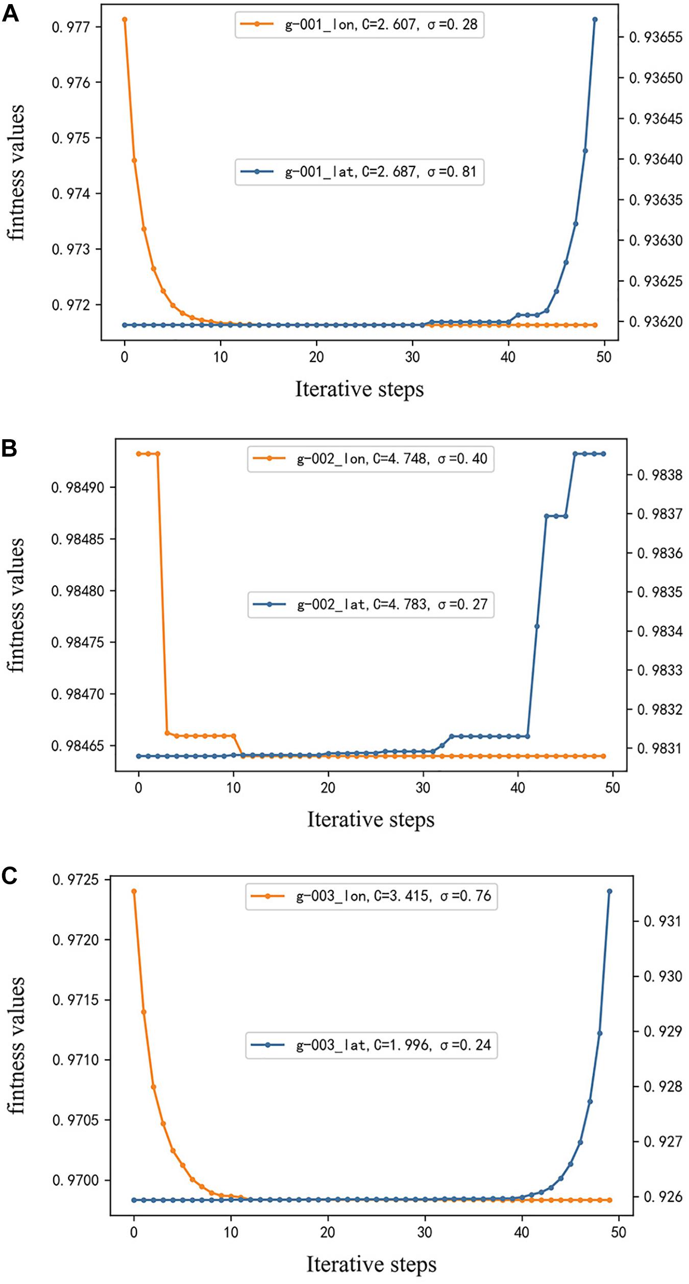
Figure 2. The relationship lines between the iterative steps and the fitness values of parameter optimization of g-001, g-002, and g-003. (A) The optimal results of parameters of g-001. (B) Represents the parameter optimization of g-002. (C) The optimal results of parameters of g-003. The yellow line represents the fitness values in the longitudinal direction, and the blue line demonstrates the fitness values in the latitudinal direction; the legends demonstrate the best hyperparameters.

The Comparative Experiment Results

To verify the effectiveness and stability of our model, we conduct comparison experiments with four baselines, random forest (RF), K-nearest neighbor (KNN), AdaBoost (Ada), and the basic SVR, respectively.

Figure 3 shows the test regression results of three glider datasets by using RF, KNN, Ada, SVR, and PSO-SVR, respectively. Figures 3A–C demonstrate the real trajectories and predicted trajectories of g-001, g-002, and g-003, respectively. Since the difference between the results regressed by several methods is not obvious enough and the trajectories of gliders are not regular, we have to add the comparison experiments of the errors between predicted values and real values to validate the results. Figures 3D–F introduce the error comparison results. The errors are computed by the function as follows:

$$error=\sqrt{{\left(pre{d}_{lon}-rea{l}_{lon}\right)}^2+{\left(pre{d}_{lat}-rea{l}_{lat}\right)}^2}(9)$$

FIGURE 3

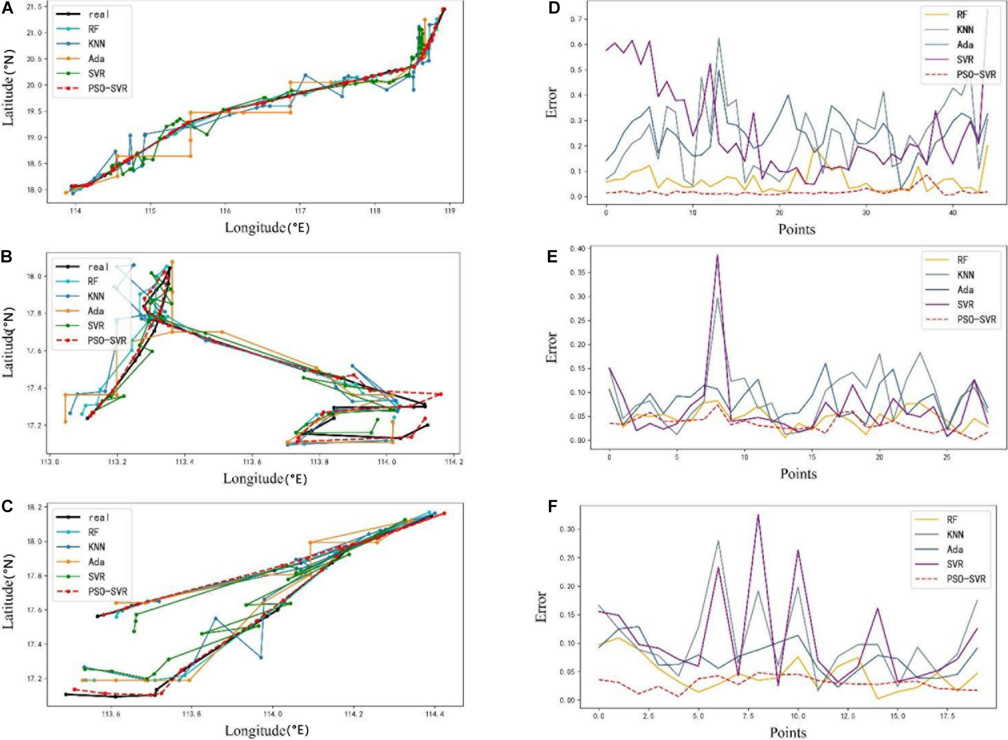
Figure 3. The comparisons of the trajectories of three gliders reconstructed by several algorithms with the original trajectories and the error comparisons between the proposed model with the comparison models. (A) The comparison of the regression results of g-001. (D) The comparison of the error of g-001. (B) The comparison of the regression results of g-002. (E) The comparison of the error of g-002. (C) The comparison of the regression results of g-003. (F) The comparison of the error of g-003.

Cooperating the figures of trajectory comparison in conjunction with the figures of error comparison, we can learn that the trajectory predicted by the simulation model proposed by us has the best fit with the real trajectory, and what is completely different from other methods is that the proposed model keeps a stable and slight error which confirms the robustness of our model.

Based on the simulation information of PSO-SVR and other comparative experiments, we can further evaluate the effectiveness and stability of the proposed simulation model by the mean square error (MSE), the relative error (RE), and the coefficient of determination (R2).

$$MSE=\frac{1}{N}\sum _{i=1}^N{\left(y_i-f\left(x_i\right)\right)}^2(10)$$

$$RE=\frac{||y_i-f(x_i)||}{y_i}(11)$$

$$R2=\frac{{\sum }_i^N{\left(f\left(x_i\right)-\overline{y_i}\right)}^2}{{\sum }_i^N{\left(y_i-\overline{y_i}\right)}^2}(12)$$

Here, y_i denotes the real position that the glider comes out of the water, f(x_i) is the location of the glider predicted by the simulation model. The quantity $\overline{y_i}$ is the mean value of y_i over the whole moving process. N is the number of test samples.

The MSE, RE, and R2 over the testing samples of three glider datasets are shown in Figure 4. Figure 4A represents the performance of the simulation model applied in g-001 where MSE = 0.00039, RE = 0.0005, and R2 = 0.9998; Figure 4B shows the assessment factors of g-002 where MSE = 0.00095, RE = 0.0013, and R2 = 0.993; the results of g-003 can be found in Figure 4C, the value of MSE is 0.0007, RE is 0.0012, and R2 is 0.994. Obviously, in contrast to other methods, the PSO-SVR yields better regression results with the lowest MSE and RE and the highest R2, and these assessment indicators demonstrate that the simulation model can accurately predict the trajectories of gliders and meet the key idea of our experiments.

FIGURE 4

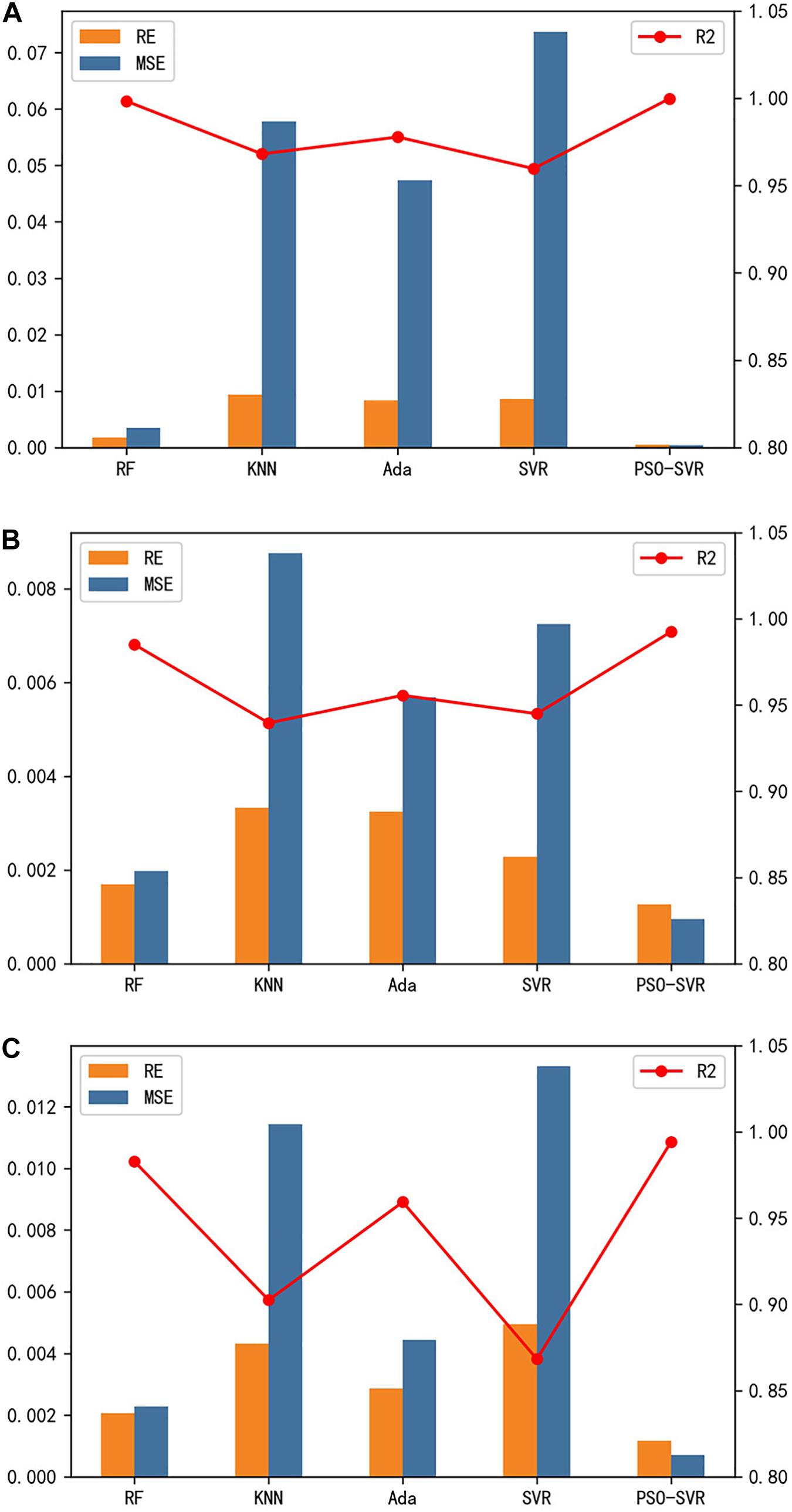
Figure 4. The performances of the model constructed by RF, KNN, Ada, SVR, and PSO-SVR, respectively. (A) The performances of the model constructed with the dataset of g-001. (B) The performances of the model constructed with the dataset of g-002. (C) The performance of the model constructed with the dataset of g-003. The orange histogram represents the relative errors (RE), and the blue histogram shows the mean square error (MSE). The coefficient of determination (R2) of the models is represented by the red line.

We can find out that the simulation model tested on the same type of gliders has a different level of performance. The mode tested with g-001 has the best performance, the performance on g-003 is second, and g-002 has the worst performance. From the information obtained from Figure 1, the strength of the geostrophic currents of the g-001 trajectory coverage is much lighter than that of g-002 and g-003. Besides, we can learn that the movement direction of g-003 is consistent with the direction of the flow field, while the direction of g-002 is opposite to the flow field which makes the simulation model with g-003 have better performance. Further speaking, both g-001 and g-003 conduct the experiment for crossing the eddy, but g-001 only conducts cross-sectional observation, and the level at which g-001 is affected by the ocean dynamic process is much weaker than that of g-003, which makes the model test with g-001 have better performance than that with g-003.

Besides, the error curves of the PSO-SVR algorithm in Figures 3D–F have many bumps. Analyzed in conjunction with Figure 1, the bump in the g-001 simulation experiment appears when g-001 crossed through the eddy. The bumps in the g-002 simulation experiment mostly appear at the intersection of trajectories and the period of reverse movement. In the simulation experiment of g-003, the larger error values are distributed when the glider sails to the boundary of the eddy.

From the above discussion, we suppose that the strength and direction of the flow field play an indispensable role in the accuracy of the simulation model. The strong currents, to a certain extent, reduce the performance of the simulation model. The eddies also have a great influence on the effectiveness of the simulation model. When the gliders cross over the eddies or move to the boundary of the eddies, the performance of the model will decrease. Meanwhile, comparing g-002 with g-003, the difference between them is small which may be caused by their different weights.

Conclusion

The tremendous potential value of the ocean observation with the glider arrays is well known. However, the strong, variable ocean currents, the lack of real-time feedback information of gliders, and the high cost of cooperative observation with glider arrays make it necessary to design a simulation model to provide strategies for the deployment and adjustment of glider arrays. The main target of our simulation model is to assimilate the data collected by gliders into numerical models and model rapidly to predict the future trajectories of glider arrays in advance which can direct the gliders more efficiently to adjust measurement formation. In this model, we collected three main influence factors, including the strength and direction of ocean currents, the current coordinate of the glider, and the diving depth of the glider, to predict the trajectory of the glider after working for a certain period of time. In addition, in the case that the accuracy of the datasets is high enough, other more valuable factors can be introduced. Moreover, to improve the performance of our model, we use the PSO algorithm to dynamically optimize the hyperparameters of the SVR algorithm and then cooperate PSO with SVR as the supporting algorithm of the simulation model.

We conducted the experiments to demonstrate the effectiveness of the model by applying the model to sea-wing gliders. The results show that the simulation model has good performance on sea-wing underwater gliders. However, we need more datasets to evaluate the performance of the model applied on different makes of gliders.

Data Availability Statement

The data analyzed in this study is subject to the following licenses/restrictions: The datasets analyzed in this article are not publicly available. Requests to access these datasets should be directed to yufangjie@ouc.edu.cn.

Author Contributions

FY and GC conducted the analysis on the datasets of the gliders and led the design of the simulation model. ZZ performed the run of the model. FY and ZZ wrote the first draft. JY validated and refined the algorithm. All authors reviewed, edited the final manuscript, and conceived the research question.

Funding

This research was jointly supported by the National Key Research and Development Program of China under contract nos. 2016YFC1402608 and 2019YFD0901001 and the Marine S&T Fund of Shandong Province for Pilot National Laboratory for Marine Science and Technology (Qingdao), grant no. 2018SDKJ0102-7.

Conflict of Interest

The authors declare that the research was conducted in the absence of any commercial or financial relationships that could be construed as a potential conflict of interest.

Acknowledgments

The study benefited from the glider datasets collected by Shenyang Institute of Automation, Chinese Academy of Sciences, Shenyang, China.

Footnotes

1. ^ https://www.aviso.altimetry.fr/

References

Brereton, R. G., and Lloyd, G. R. (2010). Support vector machines for classification and regression. Analyst 135, 230–267.

Google Scholar

Clark, E. B., Branch, A., Chien, S., Mirza, F., Farrara, J., Chao, Y., et al. (2020). Station-keeping underwater gliders using a predictive ocean circulation model and applications to SWOT calibration and validation. IEEE J. Ocean. Eng. 45, 371–384. doi: 10.1109/joe.2018.2886092

CrossRef Full Text | Google Scholar

Fonti, A., Freddi, A., Longhi, S., and Monteriù, A. (2011). Cooperative and decentralized navigation of autonomous underwater gliders using predictive control. IFAC Proc. Vol. 44, 12813–12818. doi: 10.3182/20110828-6-it-1002.02980

CrossRef Full Text | Google Scholar

Jiang, M., Jiang, S., Zhu, L., Wang, Y., Huang, W., and Zhang, H. (2013). Study on parameter optimization for support vector regression in solving the inverse ECG problem. Comput. Math. Methods Med. 2013:158056.

Google Scholar

Kennedy, J., and Eberhart, R. (1995). “Particle swarm optimization,” in Proceedings of ICNN’95 - International Conference on Neural Networks (Perth, WA: Institute of Electrical and Electronics Engineers).

Google Scholar

Kim, D., Lee, S., and Lee, J. (2020). Data-driven prediction of vessel propulsion power using support vector regression with onboard measurement and ocean data. Sensors 20:1588. doi: 10.3390/s20061588

PubMed Abstract | CrossRef Full Text | Google Scholar

Leonard, N. E., Paley, D. A., Davis, R. E., Fratantoni, D. M., Lekien, F., and Zhang, F. (2010). Coordinated control of an underwater glider fleet in an adaptive ocean sampling field experiment in monterey bay. J. Field Robot. 27, 718–740. doi: 10.1002/rob.20366

CrossRef Full Text | Google Scholar

Leonard, N. E., Paley, D. A., Lekien, F., Sepulchre, R., Fratantoni, D. M., and Davis, R. E. (2007). Collective motion, sensor networks, and ocean sampling. Proc. IEEE 95, 48–74. doi: 10.1109/jproc.2006.887295

CrossRef Full Text | Google Scholar

Li, S., Wang, S., Zhang, F., and Wang, Y. (2019). Constructing the three-dimensional structure of an anticyclonic eddy in the south china sea using multiple underwater gliders. J. Atmos. Ocean. Technol. 36, 2449–2470. doi: 10.1175/jtech-d-19-0006.1

CrossRef Full Text | Google Scholar

Liblik, T., Karstensen, J., Testorc, P., Aleniusd, P., Hayese, D., Ruizf, S., et al. (2016). Potential for an underwater glider component as part of the global ocean observing system. Methods Oceanogr. 17, 50–82. doi: 10.1016/j.mio.2016.05.001

CrossRef Full Text | Google Scholar

Paley, D. A., Zhang, F., and Leonard, N. E. (2008). Cooperative control for ocean sampling: the glider coordinated control system. IEEE Trans. Control. Syst. Technol. 16, 735–744. doi: 10.1109/tcst.2007.912238

CrossRef Full Text | Google Scholar

Rao, D., and Williams, S. B. (2009). Large-scale path planning for Underwater Gliders in ocean currents.

Google Scholar

Rudnick, D. L., Davis, R. E., Eriksen, C. C., Fratantoni, D. M., and Perry, M. J. (2004). Underwater gliders for ocean research. Mar. Technol. Soc. J. 38, 73–84.

Google Scholar

Shu, Y., Chen, J., Li, S., Wang, Q., Yu, J., and Wang, D. (2019). Field-observation for an anticyclonic mesoscale eddy consisted of twelve gliders and sixty-two expendable probes in the northern South China Sea during summer 2017. Sci. China Earth Sci. 62, 451–458. doi: 10.1007/s11430-018-9239-0

CrossRef Full Text | Google Scholar

Smola, A. J., and Scholkopf, B. (2004). A tutorial on support vector regression. Stat. Comput. 14, 199–222. doi: 10.1023/b:stco.0000035301.49549.88

CrossRef Full Text | Google Scholar

Testor, P., de Young, B., Rudnick, D. L., Glenn, S., Hayes, D., Lee, C. M., et al. (2019). OceanGliders: a component of the integrated GOOS. Front. Mar. Sci 6:422. doi: 10.3389/fmars.2019.00422

CrossRef Full Text | Google Scholar

Thompson, D. R., Chien, S., Chao, Y., Li, P., Cahill, B., Levin, J., et al. (2010). “Spatiotemporal path planning in strong, dynamic, uncertain currents,” in Proceedings of the IEEE International Conference on Robotics and Automation ICRA (Anchorage, AK: Institute of Electrical and Electronics Engineers), 4778–4783.

Google Scholar

Xiong, C., Zhou, H., Lu, D., Zeng, Z., Lian, L., and Yu, C. (2020). Rapidly-exploring adaptive sampling tree^∗: a sample-based path-planning algorithm for unmanned marine vehicles information gathering in variable ocean environments. Sensors 20:2515. doi: 10.3390/s20092515

PubMed Abstract | CrossRef Full Text | Google Scholar

Xue, D. Y., Wu, Z. L., Wang, Y.-H., and Wang, S.-X. (2018). Coordinate control, motion optimization and sea experiment of a fleet of petrel-II gliders. Chin. J. Mech. Eng. 31:17.

Google Scholar

Zhang, F., Fratantoni, D. M., Paley, D. A., Lund, J. M., and Leonard, N. E. (2007). Control of coordinated patterns for ocean sampling. Int. J. Control 80, 1186–1199. doi: 10.1080/00207170701222947

CrossRef Full Text | Google Scholar