Data-Driven Mapping With Prediction Neural Network for the Future Wide-Swath Satellite Altimetry

Two-dimensional mapping of sea surface height (SSH) for future wide-swath satellite altimetry (WSA) is a challenge at present. So far, considering the utilization of data-driven methods is a new researching direction for SSH mapping. In general, the data-driven mapping methods rely on the spatial-temporal relationship of the observations. These methods require training in large volumes, and the time cost is high, especially for the WSA observations. This paper proposed the prediction neural networks for mapping (Mapping-PNN) method to improve the training efficiency and maintain stable data and mapping capabilities. By 10-year wide-swath satellite along track observing system simulation experiments (OSSEs) on the HYCOM data, the experiment results indicate that the method introduced in this paper can improve the training efficiency and meet the grid mapping expectations. Compared with other methods, the root mean squared error (RMSE) of the mapping-PNN method can be limited within the range of ~1.8 cm, and the new method can promote the observation of the ocean phenomena scale with < ~40 km, which reaches state of the art.

Introduction

The 2D SSH mapping is a big challenge for future WSA, which is a major topic of discussion nowadays. The wide-swath satellite missions, such as the surface water and ocean topography (SWOT) mission of the US-France (Gaultier et al., 2016) and the Guanlan satellite mission of China (Chen et al., 2019) will provide 2D altimetric information with a high resolution [15–30 km, depending on sea state (Morrow et al., 2019)]. At present, the optimal interpolation (OI) method (Le Traon et al., 2003) and the dynamic interpolation (DI) method (Ubelmann et al., 2015) are the main classical model-driven two-dimensional data mapping methods (Lguensat et al., 2017) for the altimetric satellite observations [such as the products of the AVISO (Archiving, Verification and Interpretation of data of Satellites Oceanography, CollecteLocalisation Satellites (CLS), AVISO, CNES, 2019)]. The OI method, a static, statistical data mapping approach based on the objective analysis method (Bretherton et al., 1976), with the combined observations of multiple satellites (Morrow and Traon, 2012; Amores et al., 2018; Ballarotta et al., 2019), the SSH grid data products could acquire mesoscale ocean phenomena larger than ~150 km scales or longer than ~10 days (Dussurget et al., 2011; Morrow et al., 2019) but cannot observe short-period and small-scale ocean dynamic phenomena (Morrow et al., 2019; Guillou et al., 2020). However, through the OI method with the WSA OSSEs, more details of ocean dynamic phenomena and sub-mesoscale ocean phenomena could be observed, such as the scale ranges from ~25 to ~150 km (Ma et al., 2020). The DI method, which is based on the potential vorticity (PV) conservation theory (Hua and Haidvogel, 1986; Wunsch and Carl, 1996), can be adopted to observe instantaneous nonlinear ocean dynamic phenomena and express them through data reconstruction (Ubelmann et al., 2016), but it may fail to achieve acceptable results when trying to reconstruct the coastal regions or the tropic regions (Roge et al., 2017; Ballarotta et al., 2020). Those classical model-driven methods could be utilized to obtain SSH grid data products for the future WSA.

However, there are some detailed problems in the process of mapping by OI methods, such as eddies missing or the generation of “artifact” eddies (Ma et al., 2020). The DI method has limitations on mapping the sea areas where the PV conservation fails (Roge et al., 2017; Ballarotta et al., 2020). Then, consequently, the “data-driven” mapping methods (Lguensat et al., 2017, 2019b; Zhen et al., 2020) are proposed. Unlike the classical model-driven methods (Lguensat et al., 2017), the data-driven methods rely on the spatial-temporal relationship of the observations (Lguensat et al., 2019b).

Lguensat et al. (2017), who used machine learning (ML) methods in the Mediterranean, South China sea area (Lguensat et al., 2019b), and the Gulf of Mexico (Zhen et al., 2020) through principal component analysis (PCA), K nearest neighbor (KNN), and k-dimensional tree (KD-Tree) technologies, introduced a data-driven mapping method named AnDA (Lguensat et al., 2017). Furthermore, Lopez-Radcenco et al. (2019) extended the AnDA method to the mapping for multi-satellite-combined observations, SWOT observing system simulation experiments (OSSEs)-simulated data, as well as the combination of observations of nadir altimeter satellites and SWOT, and then obtained higher-accuracy SSH grid data products than the result of the OI method (Lopez-Radcenco et al., 2019). By utilizing deep learning (DL) for the DI theory verification in North Atlantic regions, Lguensat et al. (2019a) proved that the combination of the DI method and DL is feasible for data mapping. Compared with the result of the DI method on instantaneous nonlinear data, the accuracy and the error are similar for the data products obtained by “data-driven” methods, machine learning, and deep learning. According to the validation by DL, the DI method is reliable for the instantaneous nonlinear ocean dynamic signals inversion in the active ocean phenomenon regions (Lguensat et al., 2019a).

Shi et al. (2015) proposed the convolutional long short-term memory (ConvLSTM) deep learning method. This approach uses the convolution neural network (CNN) activation method, instead of the rectified linear unit (RELU) or Sigmoid activation functions, to improve the prediction performance in each gate of the classical LSTM network (Hochreiter and Schmidhuber, 1997). The advantage of CNN is that the feature extraction ability of LSTM can be enhanced. Inspired by the ConvLSTM neural network, Lotter et al. (2017) proposed the PredNet method, which grafts the ConvLSTM network to the C gate (the Gates of Controller), further improves the feature extraction ability of the predictive neural network, and makes it more accurate and reliable (Lotter et al., 2017). At the same time, the PredNet method is effective in predicting rapidly changing images and video transport streams (Lotter et al., 2017). Deep learning algorithms have been used for oceanographic applications, such as classification, identification, and prediction. Besides, Lima et al. (2017) used a CNN to identify ocean fronts, which yielded a higher recognition accuracy than the traditional algorithms. Yang et al. (2018) established a sea surface temperature (SST) prediction model based on LSTM networks that have been well tested using coastal SST data of China. By training 20-year AVISO grid data, Ma et al. (2019) used PredNet to conduct DL and implement daily ocean eddy forecast. It was proved that DL could be available on ocean observation prediction.

The purpose of this paper is to find a new 2D mapping method for future WSA observations and to map high-precision, low-error SSH grid data products for future altimetric satellites.

Based on the high-resolution model, this paper puts forward a new “data-driven” mapping method, prediction neural networks for mapping (Mapping-PNN) method by training the OSSEs along-track sampled data of WSA year by year. Additionally, the least recently used access (LRUA) module proposed by Santoro et al. (2016) is adopted, and it is a pure content-based memory write unit that writes memories to either the least used memory location or the most recently used one (Santoro et al., 2016). As for the Mapping-PNN test, it could obtain RMSE result similar as the PredNet method and better than the AnDA method, meeting the expectations. According to the results of experiments, by using the same sampled data volumes of the WSA in the region of Kuroshio and the Kuroshio Extension on OSSEs and testing three data mapping methods, the RMSE result of 2D mapping products can be limited within the range of ~1.8 cm.

The experiment verification indicates that the Mapping-PNN method is applicable to the 2D mapping for WSA. Compared with the results of the ML method (Lguensat et al., 2017) and the DL method (Lotter et al., 2017), the Mapping-PNN method has the same data-mapping capabilities. It can obtain not only high-precision, high-resolution SSH grid data product with a high rate and low error but also promote the ability of the observation for the scales with < ~40 km.

The remaining sections of this paper are arranged as follows: Material section describes the test materials and data. Methods section introduces the method of this paper. Experiment section illustrates the experiments and results. Conclusion and Discussion section is the conclusion, discussion, and the introduction of the future work.

Materials

Model Data of HYCOM

The data set of hybrid coordinate ocean model (HYCOM) has a resolution of 1/12.5° × 1/12.5°. The Kuroshio and the Kuroshio Extension regions (the sea area researched in this paper at 15°E−39°E, 120°N−144°N region) belong to the middle latitude range. There are seasonal variations of the ocean phenomena in the Kuroshio and the Kuroshio extension regions. Specifically, the seasonal variation of the Kuroshio and the Kuroshio extension is affected by both dynamic factors (SST advection and vertical temperature transport) and thermal factors (net heat flux at the air-sea interface) (Itoh, 2010; Nagano et al., 2013). The ocean phenomena of the Kuroshio and the Kuroshio extension increase significantly at the end of February in winter and strengthen continuingly in spring (Ji et al., 2018). The absolute geostrophic velocity extreme value of the Kuroshio extension appears slightly later than the Kuroshio (Nagano et al., 2013). The HYCOM data cover the global region, which is conducive to implementing the mapping simulation works in different target sea regions. The HYCOM data, as the representative model data in the application of OSSEs, are updated annually and made available to the public and facilitate scientific research and mutual verification of peer work. Meanwhile, HYCOM is a part of the Global Ocean Data Assimilation Experiment (GODAE) of the United States (Hybrid Coordinate Ocean Model (HYCOM) Data., 2021). The temporal resolution of HYCOM data for training is daily. In general, the HYCOM real-time high-resolution model includes three-dimensional ocean state description, the local coastal model, and the global coupled ocean-atmosphere prediction model with a prescribed ocean boundary.

The Parameters of Guanlan Mission

The 791-Orbit of Guanlan (Chen et al., 2019) was utilized in the experiment. The altitude of 791-Orbit is 791.254 km, which ensures a high observation swath of the WSA and provides the parameters for the OSSEs of the HYCOM. The parameter for generating the input sources of the OSSEs, including the exact repeat cycle, the sub-cycle, the orbit altitude, and the swath width, is required to participate in the calculation process of the along-track sampling simulations. The exact repeat cycle of 791-Orbit is approximately 14 days (4-day sub-cycle) over a swath width of 166.4 km (with a gap width of 27.6 km). A sub-cycle is an integer number of days; after which, the ground track of a satellite repeats itself within a small offset. In other words, a sub-cycle can be viewed as a near-repeat cycle with duration equaling to an integer number of nodal days (Pie and Schutz, 2008). And 4-day-long sub-cycle is chosen for OSSEs in the paper according to the 791-Orbit.

Data of the Simulation Experiment

According to the orbit of the Guanlan satellite and its parameters, the swath width, the nadir gap width, the coordinates of the swath trajectory, and the gap trajectory of the satellite had been calculated. Then, combined with the OSSEs, the sampled data in one cycle were merged to generate global observations, which would be used as the input source data for the subsequent mapping process. In the OSSEs, the data of each orbit on each cycle were calculated by the satellite track analysis algorithms by using reasonably matched satellite parameters.

As shown from Figure 1A represents the data sampling simulation in the OSSEs, using the parameter of the 791-Orbit, and the figure shows four ascending-descending tracks in one cycle. Figure 1B is an example of a one-cycle data sampling simulation according to the 14-day in one cycle of the 791-Orbit. And Figure 1C illustrates one-cycle Global OSSEs results in grids. Figure 1 is an example of the sampled observations region in the West Pacific Ocean (WPO) to show the results of OSSEs [As shown in Figures 1B,C; see details in Figures 4, 5 of Experiments section]. In the OSSEs, when the grid points are at the same longitude–latitude, only the data of the last pass through are retained. And the data of the region blocked in blue are the researching sea area in this paper, at 15–39°E, 120–144°N, which is the training, evaluation, and testing volumes for comparison of mapping methods.

FIGURE 1

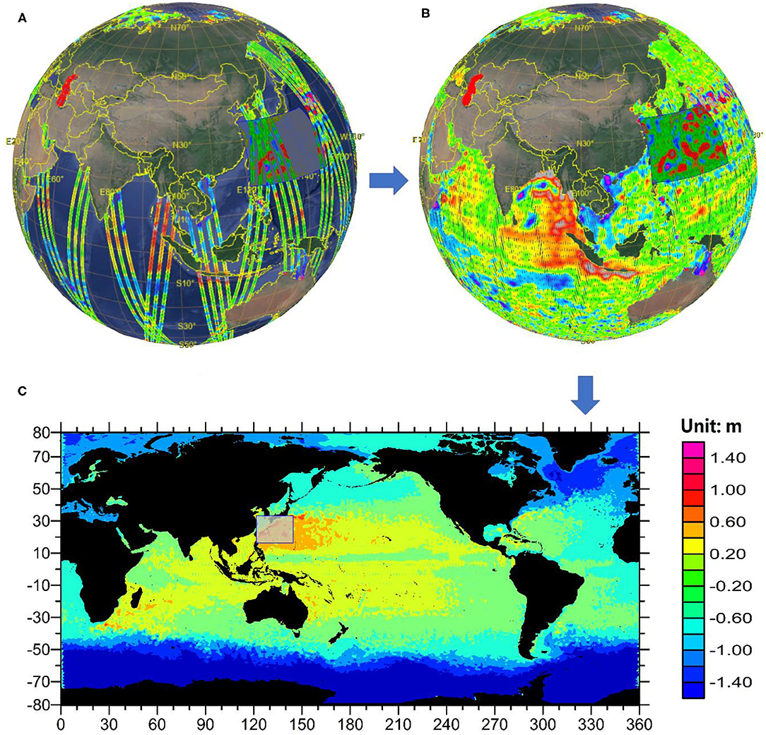
Figure 1. (A) The example of along-track SSH data; (B) An example of one-cycle sampling simulation; (C) Obtained from the data projection of (B) onto a 2D plane.

Methods

The Analog Data Assimilation (AnDA)

The observation data volumes can be organized and calculated as follows, according to the AnDA method proposed by Lima et al. (2017).

The following discrete state space (Lguensat et al., 2017):

$\begin{array}{ll}x(t)={M}[x(t-1),\eta (t)],& (1)\end{array}$

$\begin{array}{ll}y(t)={H}[x(t)]+{E}(t),& (2)\end{array}$

where time t ϵ{0, …, T} refers to the times in which observations are available, assuming the observations are at regular time steps. In Eq. (1), ${M}$ characterizes the dynamical model of the true state x(t), while η(t) is a random perturbation added to represent model uncertainty. The observation Eq. (2) describes the relationship between the observation y(t) and x(t). And the observation error is considered by the white noise ε(t). Considering an additive Gaussian noise ε with covariance T in Eq. (2) and the observation operator, the ${H}$ = H is quasi-linear (Lguensat et al., 2017).

The Eq. (1) represents the dynamical model governing the evolution of state x through time, while H is a Gaussian-centered noise of covariance Q that models the process error. And Eq. (2) explains the relationship between the observation y(t) and the state to be estimated x(t) through the operator H. The uncertainty of the observation model is represented by the e error, which is considered here to be Gaussian centered and of covariance R. The ε and H are independent, and the Q and R are known.

AnDA relies on the following state-space model, to evaluating filtering, respectively smoothing, posterior likelihood, and the distribution of the state could be estimated x(t) at time t, given past and current observations y(1, …, t), respectively given all the available observation y(1, …, T) (Lguensat et al., 2019b).

$\begin{array}{ll}x(t)={F}(x(t-1))+\eta (t)& (3)\end{array}$

$\begin{array}{ll}y(t)={H}(x(t))+{E}(t)& (4)\end{array}$

The counterpart of a model-driven operator ${M}$ of Eq. (1) is the operator ${F}$ in Eq. (3), which refers to the analog-forecasting operator. The predicting matrix could be calculated by Kalman smoother to obtain the final result (Lguensat et al., 2019b). The Kalman smoother (KS) algorithm can directly provide the optimal estimation of the state, given the observations and their corresponding errors. The AnDA method relies on the spatial-temporal relationship of the observations and introduces the analog operator through a KNN-search to make the state-space model being applied in practice.

The proceedings of the AnDA method are as follows: firstly, principal component analysis (PCA) algorithm is performed on satellite along-track sampled data obtained through OSSEs and extract data features to prepare for the later ML. Then, secondly, a KNN search in a catalog of numerical model outputs using a KD-Tree is implemented, and the final mapping result is obtained through Kalman smoothing. Readers can find the AnDA's algorithm sketch block diagram in the reference (Lguensat et al., 2017, 2019b) to learn more details about the AnDA method. This paper compares and discusses the 2D mapping capabilities of the AnDA and the Mapping-PNN methods in the experimental part (The code of python type for AnDA method can be found on the website: https://github.com/ptandeo/AnDA).

The PredNet Method

Shi et al. (2015) proposed the ConvLSTM method. In 2017, Lotter and Kreiman et al. established the PredNet neural network architecture based on ConvLSTM (Lotter et al., 2017). The theory details of ConvLSTM and PredNet are as follows:

ConvLSTM replaced each gate of the LSTM neural network (proposed by Hochreiter and Schmidhuber, 1997) with CNN architecture, which improved the ability of feature extraction for targets in the original LSTM network. The theory brief introduction and the implementation method are as follows:

ConvLSTM is an extension of full-connection LSTM (FC-LSTM), which has convolutional structures in the input-to-state and state-to-state transitions. The ConvLSTM determines the future state of a certain cell in the grid by the inputs and past states of its local neighbors. The key equations of ConvLSTM (Shi et al., 2015) are shown in Eqs. (5)–(9) below, where ‘*’ denotes the convolution operator and ‘○’ denotes the Hadamard product:

$\begin{array}{ll}{i}_t=\sigma (W_{xi}*{{X}}_t+W_{hi}*{{H}}_{t-1}+W_{ci}○C_{t-1}+b_i)& (5)\end{array}$

$\begin{array}{ll}{f}_t=\sigma (W_{xf}*{{X}}_t+W_{hf}*{{H}}_{t-1}+W_{cf}○C_{t-1}+b_f)& (6)\end{array}$

$\begin{array}{ll}{C}_t=f_t○C_{t-1}+i_t○tanh(W_{xc}*{{X}}_t+W_{hc}*{{H}}_{t-1}+b_c)& (7)\end{array}$

$\begin{array}{ll}{o}_t=\sigma (W_{xo}*{{X}}_t+W_{ho}*{{H}}_{t-1}+W_{co}○C_t+b_o)& (8)\end{array}$

$\begin{array}{ll}{{H}}_t=o_t○tanh(C_t)& (9)\end{array}$

For a spatiotemporal sequence forecasting problem, the structure consists of an encoding network and a forecasting network (Shi et al., 2015). Compared to classical LSTM, ConvLSTM can model space-time structures by encoding geographic information as tensors, thereby to overcome the limitation of losing spatial information in classic LSTM networks. Readers can find the algorithm sketch block diagram of ConvLSTM in the reference (Shi et al., 2015) to learn more details about the ConvLSTM method (The code of python type for ConvLSTM method can be found on the website: https://github.com/XingguangZhang/ConvLSTM.).

To minimize the weighted sum of the activity of the error units (Ma et al., 2019), based on the ConvLSTM concept, the network structure is enhanced to construct an improved ConvLSTM, which is named the PredNet model, for predicting sequences of images (Lotter et al., 2017). A structure in which the error is fed forward has been added to the network, as shown in Figure 2. The network consists of a series of repeatedly stacked blocks, and each of them can be viewed as one layer (Lotter et al., 2017).

FIGURE 2

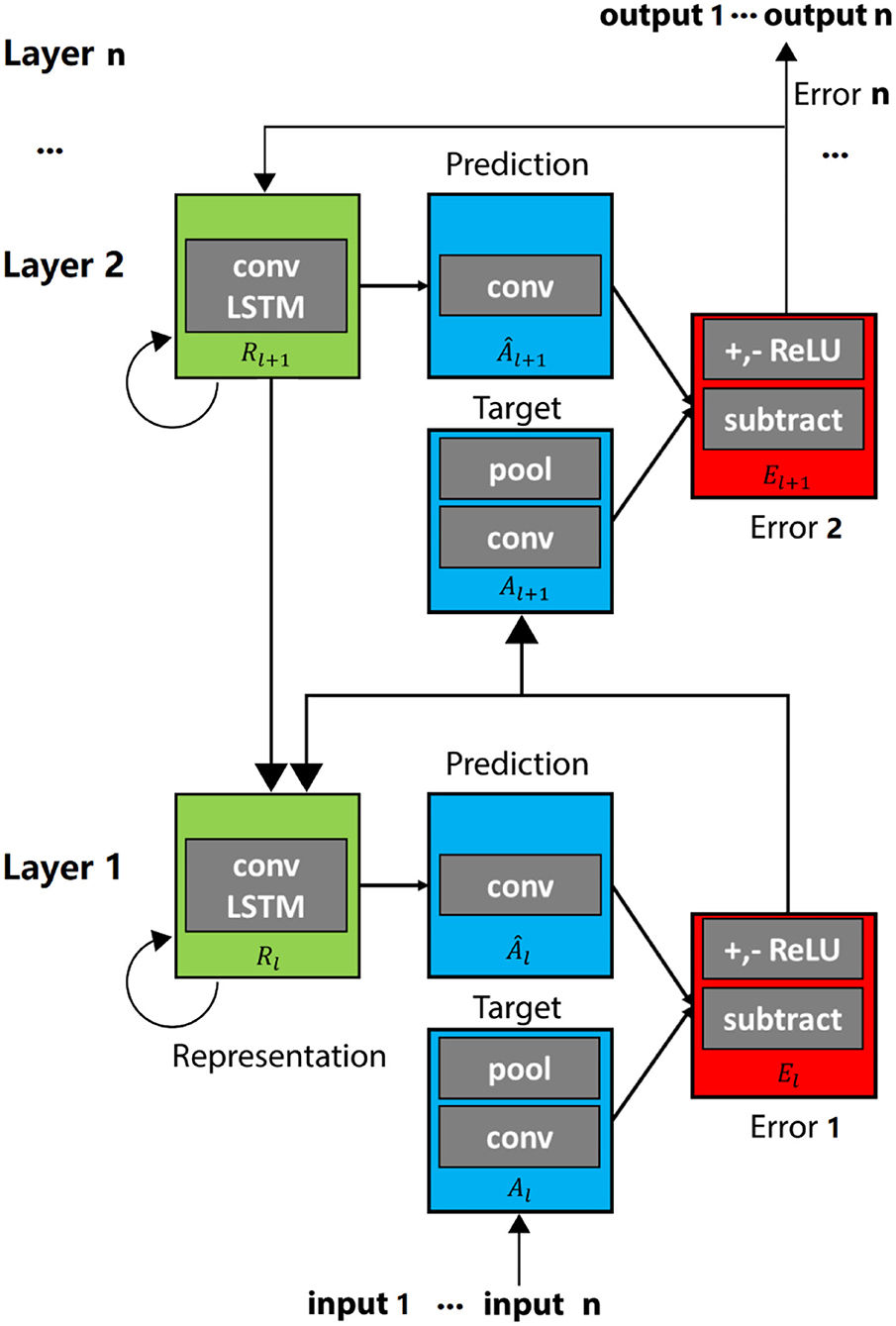
Figure 2. The sketch block diagram of PredNet.

The PredNet architecture is illustrated in Figure 2. Each module of the network consists of four basic parts: an input convolutional layer (Al), a recurrent representation layer (Rl), a prediction layer (Âl), and an error representation (El). The architecture is rooted in convolutional and recurrent neural networks (RNN) trained with back propagation (BP) (Ma et al., 2019).

$\begin{array}{ll}{A}_l^t=\{\begin{array}{c}{x}_{t}ifl=0\\ MAXPOOL(RELU(CONV(E_{l-1}^t)))l>0\end{array}& (10)\end{array}$

$\begin{array}{ll}{\widehat{A}}_l^t=RELU(CONV(R_l^t))& (11)\end{array}$

$\begin{array}{ll}{E}_l^t=\left[RELU\left(A_l^t-{\widehat{A}}_l^t\right);RELU\left({\widehat{A}}_l^t-A_l^t\right)\right]& (12)\end{array}$

$\begin{array}{ll}{R}_l^t=CONVLSTM(E_l^{t-1},R_l^{t-1},UPSAMPLE(R_{l+1}^t))& (13)\end{array}$

The full set of update rules is listed in Eqs. (10–13).

As follows, Algorithm 1 is the original PredNet algorithm.

ALGORITHM 1

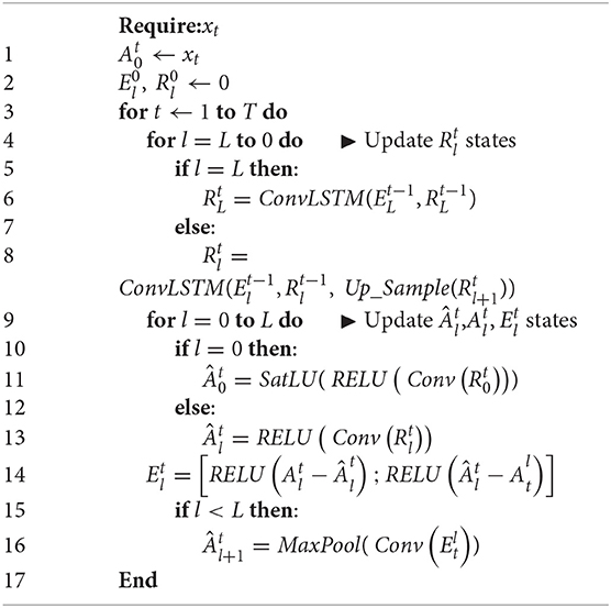
Algorithm 1: Calculation of PredNet States

Algorithm 1 was proposed by Lotter et al. (2017). The $R_l^t$states are computed, and a forward pass is initialized to calculate the predictions, errors, and higher-level targets. The initial prediction is spatially uniform (Lotter et al., 2017).

Readers can learn more details about the PredNet method in the reference (Lotter et al., 2017). This paper also compares the 2D mapping capabilities of the PredNet and the Mapping-PNN methods in the experimental part, and discusses them (The code of python type for the PredNet method can be found on the website: https://coxlab.github.io/prednet).

The Mapping-PNN Method

In the prediction of the target data, the PredNet needs a lot of learning database for the existing data set, which will increase the learning period. To improve the training efficiency of the original version of PredNet, the Mapping-PNN is proposed in this paper, and the external storage gate is added in ConvLSTM to enhance the memory and storage capacity of the learning performance of the ConvLSTM layer, accelerate the learning efficiency of the original PredNet, and save the waiting period of the observations on OSSEs. The external storage gate is utilized in the minimum training period. And the using of the least recently used access (LRUA) module helps to accelerate the read-write process of the memories. The AdamOptimizer (Kingma and Ba, 2015) is adopted to minimize the loss. The specific method is as follows.

The typical external storage gate includes duality of read and write units, as well as the external memory. The controller, neuron C_convlstm, is a ConvLSTM network, which receives the current input and controls the read units and write units to interact with the external memories, respectively. Memory encoding and retrieval in external memories are rapid, with feature representations being placed into or taken out of memory potentially every time step. Additionally, it can be used for long-term storage by slowly updating the weights and for short-term storage by external memories. Thus, when the model learns the type of representations, it will be placed into memories, and the representations will be used to implement mapping.

As shown in Figure 3, the initialized state of the Mapping-PNN network is represented by init_state. The cell state of the initialized controller, neuron C_convlstm, is represented by c_k (k = 1, 2, …, n, nϵR, and n equals to the number of the memory). Given the input SSH observations, the controller receives the memory r_t−1 and cell state c_t−1 provided by the previous state prev_state, and then produces k_convlstm used to retrieve a particular memory. Besides, the light-green arrow line represents the writing data streams, while the red arrow line illustrates the reading data streams.

FIGURE 3

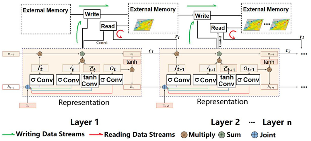
Figure 3. The sketch block diagram of Mapping-PNN.

In terms of a new sequence, it is written to a rarely used location with the recently encoded information preserved or to the last used location, which can be used for updating with newer or possibly more relevant information. Then, the whole procedure of the algorithm can be described as follows [including each component of the controller gates C_t, which is transformed from Eq. (7)]:

$\begin{array}{ll}{w}_t^u\leftarrow {\gamma }^{*}{w}_{t-1}^u+w_t^r+w_t^w& (14)\end{array}$

$\begin{array}{ll}{w}_t^{lu}(i,j)=\{\begin{array}{c}1if{w}_t^u\le m(w_t^u,n)\\ 0if{w}_t^u>m(w_t^u,n)\end{array}& (15)\end{array}$

$\begin{array}{ll}{w}_t^w\leftarrow RELU(Conv(\sigma (\alpha )•w_{t-1}^r+(1-\sigma (\alpha ))•w_{t-1}^{lu})))& (16)\end{array}$

$\begin{array}{ll}{M}_t(i,j)\leftarrow M_{t-1}(i,j)+w_t^w(i,j)•k_t& (17)\end{array}$

where w^u denotes the usage weight updated at each time step to keep track of locations most recently read or written; γ denotes the decay parameter; w^lu denotes the least-used weight computed using w^u for a given time step; the notation m(v, n) is introduced to denote the n^th smallest element of the vector v; n is set to equal the number of the writer to memory; w^w refers to the written weight computed by the function RELU(σ(.)), which combines the previous read weights w^r and previous least-used weights w^lu; α represents a dynamic scalar gate parameter to interpolate between weights. Before writing to memory, the least used memory location is computed from w^u and set to zero, and then the memory M_t is written by the computed matrix of written weights w^w. The parameters will be updated dynamically during back propagation. In addition, M_t (i, j) can be written into the zeroed memory locations or the previously used memory locations; if it is the previously used memory location, the w will simply be erased.

The memory r^t is used by the controller as both an input to a classifier and an additional input for the next input sequence. It is calculated by the Eq. (18) for prediction.

$\begin{array}{ll}{r}_t\leftarrow {\displaystyle \sum _i}{\displaystyle \sum _j}{w}_t^r(i,j)•M_t(i,j)& (18)\end{array}$

To achieve the learning, the LRUA module proposed by Santoro et al. (2016) is adopted, which is a pure content-based memory write unit that writes memories to either the least used memory location or the most recently used one (Santoro et al., 2016).

Furthermore, w^r is ConvLSTM with RELU, following the Eq. (19):

$\begin{array}{ll}{w}_t^r(i,j)\leftarrow RELU(Conv(K(k\text{\_}t,M\text{\_}t(i,j))))& (19)\end{array}$

where M_t refers to the memory matrix at time-step t, and M_t (i, j) refers to a sub-block in this matrix. The block of M_t (i, j) serves as the memory “slots,” with constituting individual memories (Santoro et al., 2016).

$\begin{array}{ll}K(k\text{\_}t,M\text{\_}t(i,j))\leftarrow LRUA(k\text{\_}t,M\text{\_}t(i,j))& (20)\end{array}$

where the read units can amplify or attenuate the precision of the focus by the read weights.

Those read weights w^r and corresponding memory M_t (i, j) are used to retrieve the memory r_t.

The ConvLSTM Layer in Algorithm 1 (Lotter et al., 2017) was optimized by the introduction of the LRUA method, and Algorithm 2 was proposed, as shown:

ALGORITHM 2

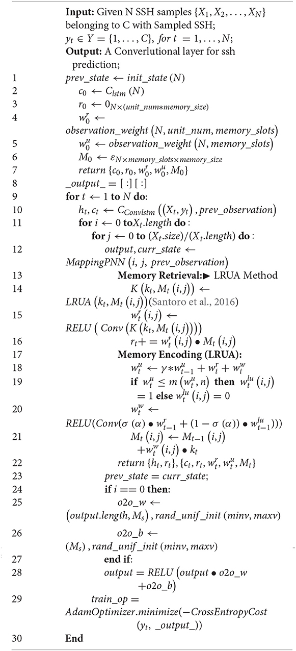
Algorithm 2: Mapping-PNN

Algorithm 2, the improvement details of the Mapping-PNN, adopted the LRUA method.

In the algorithm, the observation_weight (N, unit_num, memory_slots) function generates a tensor with the zeros set to the ones; {(N, unit_num), rand_unif _init (minv, maxv)} generates a tensor with a uniform distribution, and the value of all elements is set between minv and maxv.

For the current time-step t, the sampled data {X₁, X₂, …, X_N} and the corresponding sample-class y_t will be received by the controller C_Convlstm. The current state of the network curr_state is used by the controller as an additional input for the next time step. According to each sequence of the sample, the algorithm randomly generates the prediction label. If the sampled data X_t comes from a new observation, it will be bound to the appropriate y_t and stored by the write units in the external memory, which is presented in the subsequent time step. Once a sample from an observed-already data is presented, the controller will retrieve the bound information by the read units from the external memory for SSH prediction. The cross_entropy_cost(·) is to measure the loss between the predicted value and the correct prediction label. Then, the adaptive moment estimation, Adam,optimizer(·) (Kingma and Ba, 2015), is adopted to minimize the loss. Furthermore, the back-propagated (BP) error signal from the current prediction updates those previous weights and bias, such as the o2o_ w,o2o_ b,${\text{w}}_{\text{t}}^{\text{r}}$,${\text{w}}_{\text{t}}^{\text{w}}$ and ${\text{w}}_{\text{t}}^{\text{u}}$, followed by the updating of the external memory. Those processes would be repeated until the model converges. Meanwhile, there are some observation gaps or missing data after generation of grid SSH; therefore, an optimal interpolation is needed. The parameters, such as the coefficient matrix, the spatial distances, and searching range, will be designed based on the target region (the coefficient matrix of the observations and the errors, the range of the latitude-longitude, etc.) (Lguensat et al., 2017; Amores et al., 2018; Ma et al., 2020).

Experiments

Experimental Setups

The Regions and the Target Date

The AnDA, PredNet, and Mapping-PNN methods all need a large number of training sets during the neural network training. By utilizing 10-year HYCOM data, three data-driven methods were trained, and a target day (at the 15°E ~ 39°E, 120°N ~ 144°N region—take a date on March 1, 2017 of HYCOM for example) was considered as the target field of the experimental dataset of the three data-driven methods. The temporal resolution of test datasets is daily. The cycle of the Guanlan 791-Orbit is 14 days, and the target day is the March 1, 2017 on HYCOM. Furthermore, take the selection of the test data, for example, for AnDA, PredNet, and Mapping-PNN methods. The test data are obtained from January 1, 2017 to March 1, 2017 on HYCOM, which could be divided into “30-day data” (from January 1, 2017 to January 30, 2017) and “60-day data” (from January 1, 2017 to March 1, 2017).

The studied region in this paper is the Kuroshio region (Kuroshio extension as well). With the variation of the seasons in the northern hemisphere, the ocean phenomenon varies significantly in this region. Considering that the early stage of March is in the transition period from winter to spring, “March 1, 2017” is selected as the research target date. At this time, several new unique ocean phenomena of spring are in the generation stage, and unique ocean phenomena of winter are in the transformation stage. The illustration of the comparative analysis and research among the data mapping algorithms in the Kuroshio region and the Kuroshio extension region would be valuable for the ocean science research.

The AnDA, PredNet, and Mapping-PNN methods used 2005–2015 OSSEs observations for model training, 2015 ~2016 original data for evaluation, and 2017 original data for tests. The research on ocean phenomena represented by the Kuroshio and the Kuroshio extension is based on detailed statistics, analysis, and summary from over decades' observations. With consistency, both use the observation data as the research basis.

The evaluation and test methods of AnDA refer to the method introduced by Lguensat et al. (2017). In addition, the methods introduced by Beauchamp et al. (2020) are used as the evaluation methods of PredNet and Mapping-PNN. The validation and evaluation methods are listed in detail to evaluate the mapping performance of comprehensive indicators. For experiment results, please see The Comparison of the Experiment Results of the AnDA, the PredNet, and the 426 Mapping-PNN section.

The Hyper Parameters' Configuration

Some hyper parameters, such as optimizer and learning rate, are as follows: For the AnDA method, the error probability is 0.01. For the PredNet method and the Mapping-PNN method, to minimize the loss, an Adam,optimizer (·) is utilized, and the learning rate is 0.01 until the model converges after training 80 times in test No.1 (See Table 3 in The Comparison of the Experiment Results of the AnDA, the PredNet, and the 426 Mapping-PNN section for details). To avoid the overfitting, the early stopping strategy is utilized during the training. And if the loss of the evaluation data is no longer reduced, the training will be stopped, and the overfitting can be avoided. Meanwhile, 80 training times are the epochs when the early stopping happens.

Computer Configuration Used in This Paper (Table 1) Validation Methods

In the analysis of the experimental results, several validation methods have been used to validate the test results of three data-driven methods, such as the method of illustrating the mapping results by the figures, the absolute geostrophic velocities, the RMSE of the mapping results, the Taylor Diagram (Taylor and Karl, 2001; Beauchamp et al., 2020), the power spectral density (PSD) diagram, and the efficiency of the methods.

TABLE 1

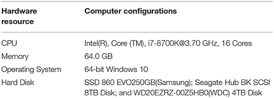
Table 1. Computer hardware resource in this paper.

The Taylor Diagram (Taylor and Karl, 2001), as an effective method, has been widely used to evaluate and verify mapping work. The correlation coefficient (COR), centered root mean square error (Centered RMSE), and standard deviation (STD) can all be expressed on Taylor Diagram and in the form of one point. The Taylor Diagram can centrally express not only the related information of multiple mapping methods but also comprehensively and clearly reflect the data reconstruction capabilities of the methods. The COR indicates the similarity between the reconstruction results and the observations. The centered RMSE represents the error difference between the mapping results and the trues. The ratio of the STD reflects the degree of dispersion between the ability to reconstruct the entire spatial data and the observations. The theoretical expressions of COR, RMSE, and STD are detailed in Eqs. (21), (22), and (23) (Taylor and Karl, 2001; Beauchamp et al., 2020; Zhen et al., 2020), respectively.

$\begin{array}{ll}STD:{\sigma }_{x\_\widehat{x}}^2(t_k)=\frac{1}{N}{\displaystyle {\sum }_{k=1}^N{[(x_k-{\widehat{x}}_k)-\overline{(x_k-{\widehat{x}}_k)}]}^2}& (21)\end{array}$

$\begin{array}{ll}COR:COR(t_k)=\frac{COV(x_k,{\widehat{x}}_k)}{\sigma (x_k)\sigma ({\widehat{x}}_k)}& (22)\end{array}$

$\begin{array}{ll}CenteredRMSE:RMSE=\sqrt{\frac{1}{N}{\displaystyle \sum _{k=1}^N}{[(x_k-\overline{x_k})-(x_r-\overline{x_r})]}^2}& (23)\end{array}$

The Comparison of the Experiment Results

Figure 4 illustrates the 2D SSH mapping results from the AnDA, the PredNet, and the Mapping-PNN in Figures 4C–E, respectively. Beyond that, Figure 4A denotes the original SSH field of HYCOM, and Figure 4B illustrates the along-track sampled data simulated from OSSEs on the date of March 1, 2017 on HYCOM, which utilized the parameter of 791-Orbit of Guanlan.

FIGURE 4

Figure 4. (A) The original SSH field of the regions on HYCOM; (B) the along-track sampled data of OSSEs on HYCOM by the parameters of Guanlan; (C) mapping result of the AnDA method; (D) mapping result of the PredNet; (E) mapping result of the Mapping-PNN method.

After the OSSEs process (Figure 4A), as the description mentioned, we used the OI as a first guess of the PredNet and Mapping-PNN methods for the gaps and missing data of the target region. By using the methods of AnDA, PredNet and Mapping-PNN, respectively, the 2D SSH grid of the 15°E−39°E, 120°N−144°N region could be obtained. The grid data are shown in Figures 4C–E, respectively.

The absolute geostrophic velocity diagram is shown in Figure 5. Figure 5A represents the absolute geostrophic velocity inversed from the original SSH field of the region (the Kuroshio and the Kuroshio extension, 15–39°E, 120–144°N region); Figure 5B represents the absolute geostrophic velocity of the AnDA method; Figure 5C represents the absolute geostrophic velocity of the PredNet method; and Figure 5D represents the absolute geostrophic velocity of the Mapping-PNN method.

FIGURE 5

Figure 5. (A) The absolute geostrophic velocity derived from Figure 4A, the original SSH; (B) the absolute geostrophic velocity from Figure 4C (the AnDA method); (C) the absolute geostrophic velocity from Figure 4D (the PredNet method); (D) the absolute geostrophic velocity from Figure 4E (the Mapping-PNN method).

As indicated in Figure 5, the absolute geostrophic velocity inversed from the Mapping-PNN method (Figure 5D) is more similar to the true value of HYCOM than the geostrophic velocity inversed from the other two methods. Compared with the AnDA method and the PredNet method, the Mapping-PNN method could obtain more small-scale ocean phenomena.

Table 2 displays the RMSE of the above test. As revealed in Table 2, the RMSE level of the 2D SSH grid data by using the methods of the three data-driven methods is basically within the range of <2 cm. The RMSE of the AnDA method, the PredNet method, and the Mapping-PNN method is 2.0, 1.8 and 1.8 cm, respectively. Therefore, the RMSE of the WSA SSH grid data products can all be limited within the range of ~1.8 cm.

TABLE 2

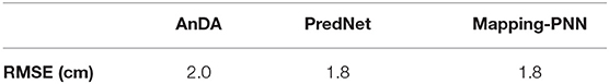
Table 2. The RMSE of the AnDA method, the PredNet method, and the Mapping-PNN method.

Figure 6 is the Taylor Diagram corresponding to AnDA, PredNet, and Mapping-PNN methods. Specifically, the red star signifies the location of HYCOM Original value on the diagram. The green dot represents the COR, RMSE, and STD location of the AnDA mapping result on the diagram. The gray dot refers to the error location of the PredNet, and the orange dot refers to the error location of the Mapping-PNN. The RMSE results of the three data-driven methods are in the range of <2 cm, which are the same as the descriptions in Table 2. The RMSE value of PredNet and Mapping-PNN is slightly better, which is in the range of 1.8 cm. In addition, the Mapping-PNN method has the same data mapping capabilities and can obtain high-precision, high-resolution SSH grid data product with a high rate and low error. As shown in Figure 6, the relative error of the Mapping-PNN method is better than that of the other methods.

FIGURE 6

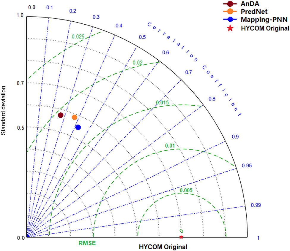
Figure 6. The Taylor Diagram computed for the AnDA, the PredNet, and the Mapping-PNN methods, respectively.

Figure 7 is the PSD diagram corresponding to AnDA, PredNet, and Mapping-PNN (M-PNN for short.) methods, respectively. The red line denotes the PSD of the HYCOM true value of the 15–39°E, 120–144°N region. The black line represents the PSD of the observations of the OSSEs, the deep-red line refers to the PSD of the mapping result from the AnDA method, the orange line is that of PredNet, and the blue line in the PSD diagram signifies the Mapping-PNN method. It shows that the Mapping-PNN method is better than the other methods for recognizing scales < ~40 km (including the sub-mesoscale, the ocean fronts, the internal waves, etc.), but the reconstruction ability of them are almost the same for the scales larger than ~40 km.

FIGURE 7

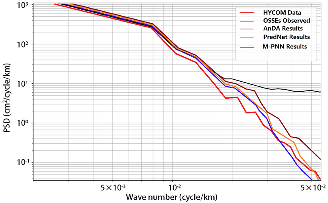
Figure 7. The PSD of the AnDA, the PredNet, and the Mapping-PNN (M-PNN for short).

In Table 3, the efficiency, accuracy, and learning rate (the error probability for AnDA) of the three data-driven methods [AnDA, PredNet, and Mapping-PNN methods (M-PNN for short)] are described to evaluate their DL ability. The continuous time of the Mapping-PNN training is better than that of the AnDA method and the PredNet method, which reaches 4 days long in test No. 1 and 6 days long in test No. 2 in the Kuroshio and the Kuroshio extension regions (from January 1, 2017 to March 1, 2017 on HYCOM). The efficiency of Mapping-PNN is higher, and the Mapping-PNN method has similar accuracy and learning rate with the PredNet method and the AnDA method.

TABLE 3

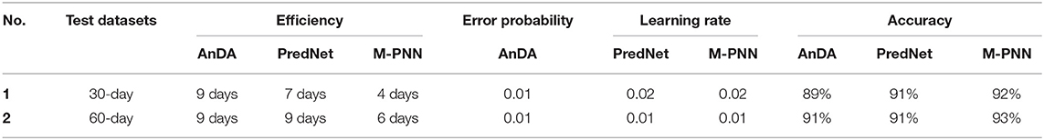
Table 3. The comparison of efficiency, error probability, accuracy, and learning rate of the three data-driven methods.

Conclusion and Discussion

Focusing on the future scientific research targets of WSA 2D mapping, this paper proposes a new data-driven mapping method called Mapping-PNN. The experiment result, which has been obtained through 10-year WSA satellite along-track OSSEs on the HYCOM data, illustrates that the method of this paper can decrease the mapping RMSE, improve the training efficiency, and meet the grid mapping expectations. Three data-driven methods (the AnDA, the PredNet, and the Mapping-PNN) were used to implement data mapping practice tests in the same region. The future satellite will provide 2D wide-swath altimetric information with an unprecedented high resolution. By comparing the three data mapping methods, this research shows that the data reconstruction ability of the Mapping-PNN method meets the WSA scientific targets.

The Mapping-PNN method proposed in this paper is evaluated with several ways, which are SSH differences, as well as the absolute geostrophic velocities differences, are illustrated with visibility analysis, and the comparisons of errors are presented with the Taylor Diagram and the PSD diagram. More specifically, the OSSEs are implemented in the same region, and the AnDA, the PredNet and the Mapping-PNN methods are used for 2D SSH Mapping. The RMSE of the three data-driven methods is at the range of <2.0 cm. Notably, the RMSE value of PredNet and Mapping-PNN is slightly better, which is in the range of ~1.8 cm. With the same data mapping capabilities, the Mapping-PNN method could obtain high-precision, high-resolution SSH grid data product. The observational dataset is based on a 14-day aggregation; considering to test other aggregation strategies, the experiments with months or seasons will be one of the future works. And, in addition, to improve the efficiency, we will use GPU(s) to implement mapping experiments in the future.

Being different from the classical model-driven method, the data-driven methods rely on the spatial-temporal relationship of the observations so that a data-driven method can capture the ocean phenomena that may not be accounted for in purely numerical models (Lopez-Radcenco et al., 2019). Moreover, the DI method (one of the model-driven methods) is based on the PV conservation theory. When sub-mesoscale ocean phenomena are < ~10 km scale, the kinetic energy is dominated by internal waves, in which the geostrophic balance fails, and the PV conservation theory is no longer applicable. And the PV conservation theory in coastal regions or the tropic regions may also fail, in which the DI method is invalid.

The data-driven method is more suitable for global 2D mapping of ocean phenomena with small scales. The data-driven and model-driven methods can be combined appropriately to obtain a new method, which not only has better mapping error accuracy than the current data-driven method but also has the common advantages of both methods. This will be a challenge for future mapping work and a research direction in the future.

One development direction of the 2D mapping method will be continuing more in-depth research along the direction of the data-driven roadmap, considering the utilization of new methods, such as generative adversarial networks (GANs) (Goodfellow et al., 2014) and enhanced networks for reinforcement learning (Huang et al., 2017), etc.

Furthermore, considering the data-driven mapping method, making error analysis of each layer (especially the hidden layer), replacing the previous BP method of individual neurons with the idea of Capsule (Sabour et al., 2017), to improve the learning rate of the entire network, and avoid the hidden dangers of invariance of CNN (Sabour et al., 2017), then obtaining data reconstruction closer to the real fields will be another research direction for future.

Data Availability Statement

The original contributions presented in the study are included in the article/supplementary material, further inquiries can be directed to the corresponding author/s.

Author Contributions

CM, JD, and GC: conceptualization. CM and JD: formal analysis, methodology, investigation, and resources. GC and CM: funding acquisition. JD: software, data curation, writing—original draft preparation, and visualization. CM: writing—review and editing. GC: supervision and project administration. All authors have read and agreed to the published version of the manuscript.

Funding

This research was funded by the Key Research and Development Program of Shandong Province: No. 2019GHZ023; National Natural Science Foundation of China: No. 41906155 and 42030406; the Fundamental Research Funds for the Central Universities: No. 201762005; and the National Key Scientific Instrument and Equipment Development Projects of National Natural Science Foundation of China: No. 41527901.

Conflict of Interest

The authors declare that the research was conducted in the absence of any commercial or financial relationships that could be construed as a potential conflict of interest.

Publisher's Note

All claims expressed in this article are solely those of the authors and do not necessarily represent those of their affiliated organizations, or those of the publisher, the editors and the reviewers. Any product that may be evaluated in this article, or claim that may be made by its manufacturer, is not guaranteed or endorsed by the publisher.

References

Amores, A., Jordà, G., Arsouze, T., and Sommer, J. (2018). Up to what extent can we characterize ocean eddies using present-day gridded altimetric products? J. Geophy. Res. Oceans 123, 7220–7236. doi: 10.1029/2018JC014140

CrossRef Full Text | Google Scholar

Archiving, Verification and Interpretation of data of Satellites Oceanography, CollecteLocalisation Satellites (CLS), AVISO, CNES. (2019). Available online at: https://www.aviso.altimetry.fr/en/home.html (accessed on 2 January 2021).

Ballarotta, M., Ubelmann, C., Pujol, M. I., Taburet, G., and Picot, N. (2019). On the resolutions of ocean altimetry maps. Ocean Sci. 15, 1091–1109. doi: 10.5194/os-15-1091-2019

CrossRef Full Text | Google Scholar

Ballarotta, M., Ubelmann, C., Rog, Marine, Fournier, F., Faugere, Y., Dibarboure, G., Morrow, R., et al. (2020). Dynamic mapping of along-track ocean altimetry: performance from real observations. J. Atmos. Ocean. Technol. 37, 1593–1601. doi: 10.1175/JTECH-D-20-0030.1

CrossRef Full Text | Google Scholar

Beauchamp, M., Fablet, R., Ubelmann, C., Ballarotta, M., and Chapron, B. (2020). Intercomparison of data-driven and learning-based interpolations of along-track nadir and wide-swath SWOT altimetry observations. Remote Sens. 12:3806. doi: 10.3390/rs12223806

CrossRef Full Text | Google Scholar

Bretherton, F. P., Davis, R. E., and Fandry, C. B. (1976). A technique for objective analysis and design of oceanographic experiments applied to mode-73. Deep-Sea Res. 23, 559–582. doi: 10.1016/0011-7471(76)90001-2

CrossRef Full Text | Google Scholar

Chen, G., Tang, J., Zhao, C., Wu, S., and Wu, L. (2019). Concept design of the “Guanlan” science mission: China's novel contribution to space oceanography (Ocean OBS19'). Front. Mar. Sci. 6, 1–14. doi: 10.3389/fmars.2019.00194

CrossRef Full Text | Google Scholar

Dussurget, R., Birol, F., Morrow, R., and Mey, P. D. (2011). Fine resolution altimetry data for a regional application in the Bay of Biscay. Mar. Geod. 34, 447–476. doi: 10.1080/01490419.2011.584835

CrossRef Full Text | Google Scholar

Gaultier, L., Ubelmann, C., and Fu, L. L. (2016). The challenge of using future SWOT data for oceanic field reconstruction. J. Atmos. Ocean. Technol. 33, 119–126. doi: 10.1175/JTECH-D-15-0160.1

CrossRef Full Text | Google Scholar

Goodfellow, I. J., Pouget-Abadie, J., Mirza, M., Xu, B., Warde-Farley, D., Ozair, S., et al. (2014). Generative adversarial networks. Adv. Neural Inf. Process. Syst. 3, 2672–2680. doi: 10.1145/3422622

CrossRef Full Text | Google Scholar

Guillou, F. L., Metref, S., Cosme, E., Sommer, J. L., and Verron, J. (2020). Mapping altimetry in the forthcoming SWOT era by back-and-forth nudging a one-layer quasi-geostrophic model. J. Atmos. Ocean. Technol. 38, 1–41. doi: 10.1175/JTECH-D-20-0104.1

CrossRef Full Text | Google Scholar

Hochreiter, S., and Schmidhuber, J. (1997). Long short-term memory. Neural Comput. 9, 1735–1780. doi: 10.1162/neco.1997.9.8.1735

PubMed Abstract | CrossRef Full Text | Google Scholar

Hua, B. L., and Haidvogel, D. B. (1986). Numerical simulations of the vertical structure of quasi-geostrophic turbulence. J. Atmos. Sci. 43, 2923–2936. doi: 10.1175/1520-0469(1986)043<2923:NSOTVS>2.0.CO;2

CrossRef Full Text | Google Scholar

Huang, V., Ley, T., Vlachou-Konchylaki, M., and Hu, W. (2017). Enhanced experience replay generation for efficient reinforcement learning. arXiv preprint arXiv: 1705.08245

Google Scholar

Hybrid Coordinate Ocean Model (HYCOM) Data. (2021). Available online at: ftp://ftp.hycom.org/datasets/GLBu0.08/expt_91.1/hindcasts/2015/ (accessed on 2 January 2021).

Google Scholar

Itoh, S. (2010). Characteristics of mesoscale eddies in the Kuroshio-Oyashio extension region detected from the distribution of the sea surface height anomaly. J. Phys. Oceanogr. 40, 1018–1034. doi: 10.1175/2009JPO4265.1

CrossRef Full Text | Google Scholar

Ji, J., Dong, C., Zhang, B., Liu, Y., and Chen, D. (2018). Oceanic Eddy characteristics and generation mechanisms in the Kuroshio Extension Region. J. Geophy. Res. Oceans 123, 8548–8567. doi: 10.1029/2018JC014196

CrossRef Full Text | Google Scholar

Kingma, D.P., and Ba, J. (2015). “Adam: a method for stochastic optimization,” in Proceedings of the International Conference on Learning Representations, San Diego, CA, USA, 7–9 May. arXiv:1412.6980

Google Scholar

Le Traon, P. Y., Faugère, Y., Hernandez, F., Dorandeu, J., Mertz, F., and Ablain, M. (2003). Can we merge GEOSTAT follow-on with TOPEX/Poseidon and ERS-2 for an improved description of the ocean circulation? J. Atmos. Ocean. Technol. 20, 889–895. doi: 10.1175/1520-0426(2003)020<0889:CWMGFW>2.0.CO;2

CrossRef Full Text | Google Scholar

Lguensat, R., Sommer, J. L., Metref, S., Cosme, E., and Fablet, R. (2019a). Learning generalized quasi-geostrophic models using deep neural numerical models. arXiv preprint arXiv: 1911.08856.

Google Scholar

Lguensat, R., Tandeo, P., Ailliot, P., Pulido, M., and Fablet, R. (2017). The analog data assimilation. Mon. Weather Rev. 145, 4093–4107. doi: 10.1175/MWR-D-16-0441.1

CrossRef Full Text | Google Scholar

Lguensat, R., Viet, P. H., Sun, M., Chen, G., and Fablet, R. (2019b). Data-driven interpolation of sea level anomalies using analog data assimilation. Remote Sens. 11:858. doi: 10.3390/rs11070858

CrossRef Full Text | Google Scholar

Lima, E., Sun, X., Dong, J., Wang, H., Yang, Y., and Liu, L. (2017). Learning and transferring convolutional neural network knowledge to ocean front recognition. IEEE Geosci. Remote Sens. Lett. 14, 354–358. doi: 10.1109/LGRS.2016.2643000

CrossRef Full Text | Google Scholar

Lopez-Radcenco, M., Pascual, A., Gomez-Navarro, L., Aissa-El-Bey, A., Chapron, B., and Fablet, R. (2019). Analog data assimilation of along-track nadir and wide-swath swot altimetry observations in the Western Mediterranean Sea. IEEE J. Selected Top. Appl. Earth Observ. Remote Sens. 12, 1–11. doi: 10.1109/JSTARS.2019.2903941

CrossRef Full Text | Google Scholar

Lotter, W., Kreiman, G., and Cox, D. (2017). Deep predictive coding networks for video prediction and unsupervised learning. arXiv preprint arXiv: 1605.08104.

Google Scholar

Ma, C., Guo, X., Zhang, H., Di, J., and Chen, G. (2020). An investigation of the influences of SWOT sampling and errors on ocean eddy observation. Remote Sens. 12, 2682–2698. doi: 10.3390/rs12172682

CrossRef Full Text | Google Scholar

Ma, C., Li, S., Wang, A., Yang, J., and Chen, G. (2019). Altimeter observation-based Eddy nowcasting using an improved ConvLSTM network. Remote Sens. 11, 783. doi: 10.3390/rs11070783

CrossRef Full Text | Google Scholar

Morrow, R., Fu, L. L., Ardhuin, F., Benkiran, M., and Zaron, E. D. (2019). Global observations of fine-scale ocean surface topography with the surface water and ocean topography (SWOT) mission (Ocean OBS19'). Front. Mar. Sci. 6, 1–19. doi: 10.3389/fmars.2019.00232

CrossRef Full Text | Google Scholar

Morrow, R., and Traon, P. Y. L. (2012). Recent advances in observing mesoscale ocean dynamics with satellite altimetry. Adv. Space Res. 50, 1062–1076. doi: 10.1016/j.asr.2011.09.033

CrossRef Full Text | Google Scholar

Nagano, A., Ichikawa, K., Ichikawa, H., Konda, M., and Murakami, K. (2013). Volume transports proceeding to the kuroshio extension region and recirculating in the Shikoku Basin. Oceanogr. J. 69, 285–293. doi: 10.1007/s10872-013-0173-9

CrossRef Full Text | Google Scholar

Pie, N., and Schutz, B. E. (2008). Subcycle analysis for Icesat's repeat groundtrack orbits and application to phasing maneuvers. J. Astronaut. Sci. 56, 325–340. doi: 10.1007/BF03256556

CrossRef Full Text | Google Scholar

Roge, M., Morrow, R., Ubelmann, C., and Dibarboure, G. (2017). Using a dynamical advection to reconstruct a part of the SSH evolution in the context of SWOT, application to the Mediterranean Sea. Ocean Dyn. 67, 1–20. doi: 10.1007/s10236-017-1073-0

CrossRef Full Text | Google Scholar

Sabour, S., Frosst, N., and Hinton, G. E. (2017). Dynamic routing between capsules. arXiv preprint arXiv: 1710.09829.

Google Scholar

Santoro, A., Bartunov, S., Botvinick, M., Wierstra, D., and Lillicrap, T. (2016). “Meta-learning with memory-augmented neural networks,” in Proceeding of the International Conference on Machine Learning, 19–24, 1842–1850. doi: 10.5555/3045390.3045585

CrossRef Full Text | Google Scholar

Shi, X., Chen, Z., Wang, H., Yeung, D.Y., Wong, W.K., and Woo, W.C. (2015). “Convolutional LSTM network: a machine learning approach for precipitation nowcasting,” in Proceedings of the Advances in Neural Information Processing Systems, Montreal, QC, Canada, 7–12, 802–810. doi: 10.5555/2969239.2969329

CrossRef Full Text | Google Scholar

Taylor, and Karl, E. (2001). Summarizing multiple aspects of model performance in a single diagram. J. Geophys. Res. 106, 7183–7192. doi: 10.1029/2000JD900719

CrossRef Full Text | Google Scholar

Ubelmann, C., Cornuelle, B., and Fu, L. L. (2016). Dynamic mapping of along-track ocean altimetry: method and performance from observing system simulation experiments. J. Atmos. Ocean. Technol. 33, 1691–1699. doi: 10.1175/JTECH-D-15-0163.1

CrossRef Full Text | Google Scholar

Ubelmann, C., Klein, P., and Fu, L. L. (2015). Dynamic interpolation of sea surface height and potential applications for future high-resolution altimetry mapping. J. Atmos. Ocean. Technol. 32, 177–184. doi: 10.1175/JTECH-D-14-00152.1

CrossRef Full Text | Google Scholar

Wunsch and Carl. (1996). The Ocean Circulation Inverse Problem. Cambridge University Press.

Google Scholar

Yang, Y., Dong, J., Sun, X., Lima, E., Mu, Q., and Wang, X. (2018). A CFCC-LSTM model for sea surface temperature prediction. IEEE Geosci. Remote Sens. Lett. 15, 207–211. doi: 10.1109/lgrs.2017.2780843

CrossRef Full Text | Google Scholar

Zhen, Y., Tandeo, P., StéphanieLeroux Metref, S., and Sommer, J. L. (2020). An adaptive optimal interpolation based on analog forecasting: application to SSH in the Gulf of Mexico. J. Atmos. Ocean. Technol. 37, 1–46. doi: 10.1175/JTECH-D-20-0001.1

CrossRef Full Text | Google Scholar