Biological Sound Sources Drive Soundscape Characteristics of Two Australian Marine Parks

McCordic, Jessica A.; DeAngelis, Annamaria I.; Kline, Logan R.; McBride, Candace; Rodgers, Giverny G.; Rowell, Timothy J.; Smith, Jeremy; Stanley, Jenni A.; Stokoe, Allison; Van Parijs, Sofie M.

doi:10.3389/fmars.2021.669412

ORIGINAL RESEARCH article

Front. Mar. Sci., 19 August 2021

Sec. Ocean Observation

Volume 8 - 2021 | https://doi.org/10.3389/fmars.2021.669412

This article is part of the Research Topic Innovation and Discoveries in Marine Soundscape Research View all 20 articles

Biological Sound Sources Drive Soundscape Characteristics of Two Australian Marine Parks

$\r\nJessica A. McCordic*$ Jessica A. McCordic^1*

Annamaria I. DeAngelis²

Logan R. Kline³

Candace McBride⁴

Giverny G. Rodgers⁴

Timothy J. Rowell²

Jeremy Smith⁴

Jenni A. Stanley⁵

Allison Stokoe¹

Sofie M. Van Parijs²

¹Integrated Statistics, Inc., Under Contract to National Oceanic and Atmospheric Administration, National Marine Fisheries Service, Northeast Fisheries Science Center, Woods Hole, MA, United States
²National Oceanic and Atmospheric Administration, National Marine Fisheries Service, Northeast Fisheries Science Center, Woods Hole, MA, United States
³Department of Wildlife, Fisheries, and Conservation Biology, University of Maine, Orono, ME, United States
⁴Parks Australia, Canberra, ACT, Australia
⁵School of Science, University of Waikato, Hamilton, New Zealand

Soundscapes represent an intrinsic aspect of a habitat which, particularly in protected areas, should be monitored and managed to mitigate human impacts. Soundscape ecology characterizes acoustic interactions within an environment, integrating biological, anthropogenic, climatological, and geological sound sources. Monitoring soundscapes in marine protected areas is particularly important due to the reliance of many marine species on sound for biological functions, including communication and reproduction. In this study we establish a baseline understanding of underwater soundscapes within two marine National Park Zones (NPZs) along the east coast of Australia: Cod Grounds Marine Park and an NPZ surrounding Pimpernel Rock within Solitary Islands Marine Park. In each of the NPZs, underwater recorders were deployed twice during the austral winter (33–35 days, 2018 and 60–69 days, 2019) and once during the austral summer (35–71 days, 2018–2019). We used the resulting acoustic recordings to determine hourly presence of anthropogenic and biological sounds between 20 Hz and 24 kHz and analyze their contributions to patterns of received sound levels. Sounds from vessels were recorded on most days throughout monitoring but were not found to influence long-term patterns of sound levels over their corresponding frequencies. Biological sources included dolphins, snapping shrimp, fish choruses, humpback whales, and dwarf minke whales. Dolphins, snapping shrimp, and fish choruses were present in all deployments. Median ambient sound levels showed a consistent diel pattern with increased levels resulting from crepuscular fish choruses combined with a higher intensity of snapping shrimp snaps during those times. Singing humpback whales strongly influenced the overall sound levels throughout the winter migration, while dwarf minke whales were consistently detected in the 2019 winter deployment but were only present in 2 h among the earlier deployments. Patterns of acoustic spectra were similar between the two NPZs, and patterns of soundscape measurements were observed to be driven by seasonal differences in biological contributions rather than anthropogenic sound sources, indicating that these NPZs are not yet heavily impacted by anthropogenic noise. These baseline measurements will prove invaluable in long-term monitoring of the biological health of NPZs.

Introduction

All marine ecosystems shoulder the burden of threats to ecosystem health, whether these impacts are direct—habitat destruction, removal of species due to fishing—or indirect—climate change, invasive species, anthropogenic noise (Halpern et al., 2007). Marine protected areas (MPAs) have been established in an attempt to minimize the effects of such threats by setting aside areas to conserve natural and cultural resources (Day et al., 2019). Although MPAs cannot fully prevent effects of larger-scale impacts such as climate change, storm damage, or global increases in underwater noise, by restricting access or usage of a targeted area, they can still provide a local refuge from many anthropogenic threats and provide a management framework for consistent monitoring efforts (Bates et al., 2019). MPAs can vary widely in size, scope, and conservation goals, but according to the IUCN, all MPAs should include goals toward conserving and improving biodiversity (Day et al., 2019). Biodiversity is declining in marine systems at a similar rate as in terrestrial systems (Polidoro et al., 2008), and there is considerable interest in monitoring MPAs to determine efficacy of regulations and management plans (Rossiter and Levine, 2014; Zupan et al., 2018).

Determining success of an MPA in terms of restoring biodiversity requires consistent monitoring as well as suitable baseline metrics to assess progress over time (Rossiter and Levine, 2014; Soga and Gaston, 2018). Biodiversity assessments are subject to shifting baseline syndrome, a phenomenon where recent environmental degradation is perceived as less detrimental due in part to a lack of awareness or recollection of historical conditions (Pauly, 1995; Soga and Gaston, 2018). For an MPA, an ideal monitoring scenario would incorporate historical data collected prior to significant human impacts to the area such as the introduction of fishing or motorized vessels (Plumeridge and Roberts, 2017), although this type of historical assessment is rarely available. Even without such historical records, however, managers can still combat shifting baseline syndrome by implementing biological monitoring regimes to collect high-quality data on current conditions that can be used as a benchmark to show trends in effectiveness of management (Rossiter and Levine, 2014; Soga and Gaston, 2018).

Consistent long-term monitoring has been cited as a key component of successful MPAs which effectively meet their conservation goals (Polidoro et al., 2008; Rossiter and Levine, 2014; Pavan, 2017); however, managers face several obstacles to effectively monitoring MPAs, including financial and logistical considerations (Day et al., 2019). MPAs present a unique set of challenges to monitoring since they often cover large areas and are remote or otherwise difficult to access, and the species of interest typically spend most if not all of their time underwater, limiting opportunities for direct observation. Most monitoring within MPAs is conducted via manned aerial or vessel patrols using visual survey methodologies including line transect surveys (e.g., Davis et al., 2004; Currie et al., 2018; Director of National Parks, 2018) or underwater visual census surveys (Edgar et al., 2004) to assess species’ presence, abundance, and distribution. Although visual methods provide high resolution information, they are necessarily restricted by safety, daylight, and personnel considerations, typically excluding observation of processes occurring at night or in inclement weather (Mellinger et al., 2007; Day et al., 2019).

Remote, autonomous passive acoustic monitoring (PAM) provides a non-invasive means of recording and archiving acoustic information gathered from the environment (Mellinger et al., 2007). This technique can be used to monitor anthropogenic noise introduced by vessels (Blair et al., 2016), sonar (Harris et al., 2018), seismic surveys (Pirotta et al., 2014), or underwater explosives (Showen et al., 2018). Many marine species including fish, invertebrates, and marine mammals produce sound in accordance with critical life functions—e.g., reproduction (Herman, 2016; Rowell et al., 2017), territory defense (Matthews et al., 2018), and foraging (Remage-Healey et al., 2006). Anthropogenic noise can impede the ability of these species to communicate, find prey, or orient themselves within the environment (e.g., Parks et al., 2009; Rossi et al., 2016). Using existing libraries of known sounds (e.g., Erbe et al., 2017) enables analysts to identify sound sources, providing a reliable way to determine presence of various taxa. Since PAM can operate continuously while deployed, it has proven to be an excellent tool for monitoring processes at various time scales such as crepuscular reef chorusing and seasonal migratory patterns of large whales (Davis et al., 2020; Mooney et al., 2020).

Along with identifying and monitoring individual sound sources, PAM can be used to collect recordings necessary to characterize an entire soundscape of an area (Pijanowski et al., 2011). Soundscape ecology incorporates a broad view of all acoustic contributions of a particular place including biological, anthropogenic, and natural abiotic sounds (Pijanowski et al., 2011). The soundscape can be thought of as an intrinsic feature of the habitat which can drive other ecological processes. In marine systems, for example, soundscape measurements have been found to correlate with larval recruitment in reef communities (Rossi et al., 2016). Characterizing the soundscape in terms of the relative contributions of various sound sources provides valuable indicators of ecologically important aspects of an area, such as biodiversity, species interactions, and degree of human disturbance (Dumyahn and Pijanowski, 2011; Pijanowski et al., 2011; Pavan, 2017; Mooney et al., 2020).

Monitoring soundscapes to determine efficacy of conservation efforts focuses on characteristics of biological and anthropogenic sources (Dumyahn and Pijanowski, 2011). Within a soundscape, species can occupy a range of acoustic niches defined by time and frequency limits which are in turn shaped by the presence of other sound sources in the soundscape (Krause and Farina, 2016; Pavan, 2017). Similar to traditional ecological niche space (Vandermeer, 1972; Pearman et al., 2008; Ricklefs, 2010), there is evolutionary pressure for assemblages of species to occupy unique acoustic niches to minimize competition for acoustic space (Krause and Farina, 2016; Tennessen et al., 2016; Wilson et al., 2020); however, novel sound sources, whether biological, anthropogenic, or climatological, can impact communication by restricting the available acoustic niche space, forcing the affected species to adjust their signals in some way or abandon the habitat altogether (Parks et al., 2009; Blair et al., 2016; Tennessen et al., 2016). In addition to acoustic disturbance, changes in soundscape characteristics may indicate response to other types of threats including habitat degradation (Coquereau et al., 2017), shifts in species composition (Butler et al., 2016; Bates et al., 2019), and ocean acidification (Rossi et al., 2016).

Monitoring soundscapes for changes in characteristics of various acoustic niches may provide an early indication of disturbance. Similar to baselines for species abundance and population monitoring, baseline metrics for soundscapes are crucial to recognizing and interpreting any changes as they relate to monitoring and managing MPAs to conserve biodiversity (Pijanowski et al., 2011; Pavan, 2017; Mooney et al., 2020). Consistent soundscape monitoring allows such changes to be placed within the context of underlying patterns due to existing biological, anthropogenic, or climatological sound sources. For example, marine soundscapes can exhibit seasonal changes due to increasing wind speeds from winter storms (Wenz, 1962; Fournet et al., 2018; Haver et al., 2019; Erbe et al., 2021b). Several field-specific metrics have been proposed to assess the partitioning of acoustic niches in time and frequency as a proxy for ecological characteristics such as biodiversity (Mooney et al., 2020). Many studies, however, rely on a collection of simpler measurements to characterize changes in a soundscape or to compare multiple soundscapes (Merchant et al., 2015; Haver et al., 2019). These include broadband sound pressure level (SPL) and power spectral density (PSD), which can be used to assess the relative acoustic pressure amplitude found in long-term recordings across different times and frequencies (Merchant et al., 2015). Both metrics provide information that is proportional to the acoustic energy in a recording; SPL provides the root-mean-square sound pressure level over the complete frequency bandwidth of recordings, and PSD provides the mean-square sound pressure level per unit frequency. Both measurements can be analyzed as a function of time or summarized over specified time intervals (Merchant et al., 2015). Measuring SPL over all frequencies and PSD over an entire deployment provides a standardized way to identify key contributors to the soundscape, compare soundscapes, and identify large-scale variations that may indicate differences due to seasons, assemblages of acoustically active species, or levels of disturbance (Dumyahn and Pijanowski, 2011; Pijanowski et al., 2011; Coquereau et al., 2017; Haver et al., 2019).

To successfully incorporate the analysis of soundscapes into MPA monitoring, measures of baseline conditions must be established. Australian Marine Parks (AMP) comprise one of the largest networks of MPAs in the world—approximately 3.3 million km²—which presents logistical challenges for monitoring both ecosystem health and compliance with regulations. The AMP system contains five marine park networks organized by geographic region and predominant marine habitat, plus the large Coral Sea Marine Park. Each of the five AMP networks contains multiple marine parks, and some parks are further subdivided into zone categories to balance conservation goals while allowing sustainable resource use (Director of National Parks, 2018; Day et al., 2019). In the present study, we seek to assess the contributors to the soundscapes and their detectable contributions to the soundscape metrics of two AMPs that have been designated as National Park Zones (NPZ)—IUCN category II. These baseline metrics can serve as a benchmark to assess the future condition of soundscapes in these MPAs to monitor efficacy of conservation efforts or evidence of increasing anthropogenic impacts.

Materials and Methods

Site Description and Recording Effort

This study focuses on two AMPs, Cod Grounds Marine Park (CGMP) and the Solitary Islands Marine Park National Park Zone (SIMP). As designated NPZs, extractive activities (e.g., fishing and mining, etc.) are prohibited, but non-extractive use (e.g., transit and tourism) is still permitted. The two NPZs are located in temperate coastal waters on the east coast of Australia and are separated by approximately 120 nautical miles (Figure 1). The entirety of CGMP is classified as an NPZ, while SIMP is comprised of a smaller (∼1 km²) NPZ within a larger AMP, the remainder of which is zoned as either Multiple Use Zone or Special Purpose Zone (IUCN category VI).

FIGURE 1

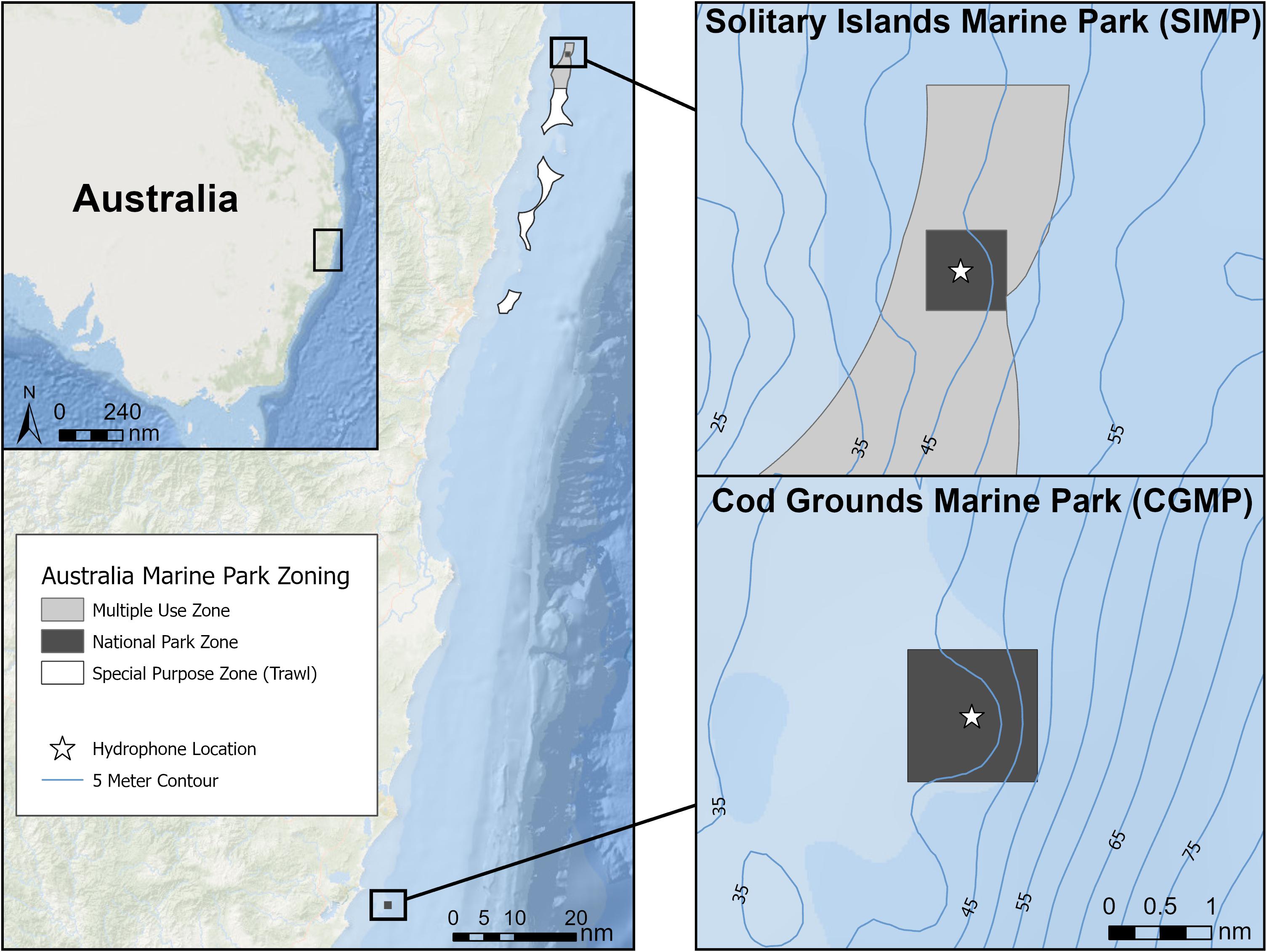
Figure 1. A map of the two study areas, Solitary Islands Marine Park (SIMP) (top right) and Cod Grounds Marine Park (CGMP) (bottom right). The entirety of CGMP is a National Park Zone (NPZ), while in SIMP the NPZ is a portion of the larger park which also contains a Multiple Use Zone (light gray) and a Special Purpose Zone (white). Hydrophone deployment locations within the two NPZs are indicated by white stars.

All recordings were made using SoundTrap 300 acoustic recorders (Ocean Instruments, Inc.) and were set to sample at 48 kHz with the high gain calibration. The manufacturer states that the SoundTrap recorders have a flat frequency response (±3 dB) between 20 Hz and 60 kHz, providing an effective recording range for this study of 20 Hz to 24 kHz (Table 1), although some frequency-dependent variations in sensitivity may exist. Using a VEMCO Ascent acoustic release mechanism, SoundTraps were attached 2–3 m above a fixed mooring (depth = 37 m CGMP, 42 m SIMP) with subsurface floats extending ∼ 6 m vertically into the water column. Within SIMP, a hydrophone was deployed to the west of Pimpernel Rock on a hard reef substrate (see Kline et al. (2020) for detailed site description). In CGMP, a hydrophone was deployed on a sandy bottom. Hydrophones were deployed three times at each site between July 2018 and August 2019 to capture seasonal variation of the underwater soundscapes within the NPZs. In the first deployment (D1: winter 2018–2019), recorders were set to record continuously. In the second and third deployments (D2: summer 2019 and D3: winter 2019), recorders were set to record with a duty cycle of 30 min of recording followed by a 30-min non-recording period each hour to extend battery life. Specific deployment dates varied by site, ranging from 32 to 74 recording days per deployment (Table 1).

TABLE 1

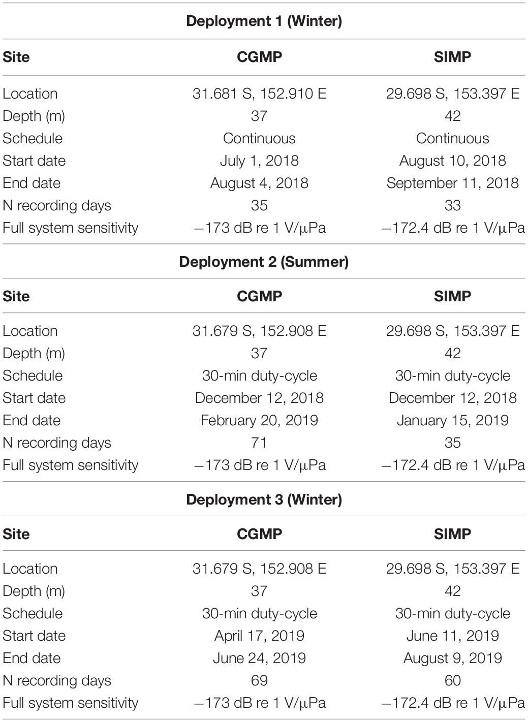
Table 1. Summary of passive acoustic recording effort in Cod Grounds Marine Park (CGMP) and Solitary Islands Marine Park National Park Zone (SIMP).

Presence of Sound Sources

Hourly Presence

Trained analysts manually reviewed all acoustic data using spectrograms generated in Raven Pro 2.0 (Center for Conservation Bioacoustics, 2014) to determine the hourly presence of anthropogenic and biological sound sources, which was in turn used to assess seasonal and diel patterns of each source. Although the 30-min duty cycle used in D2 and D3 may result in fewer total observations, it is robust to detecting patterns of presence at the time scales used in analysis (Thomisch et al., 2015). Selection boxes were drawn tightly around each signal of interest, and selection tables were generated in Raven Pro containing upper and lower frequency limits (Hz) for each event.

Consistent with methods described in Kline et al. (2020), vessels were considered present if the acoustic signature of the vessel included visually discernible acoustic pressure-squared amplitude > 500 Hz. The 500 Hz cutoff was used as a conservative measure to avoid inclusion of vessels that were too far away to reliably discern the signal from background noise. Based on preliminary analysis of the recordings as well as an existing survey of acoustically active marine mammals of Australia (Erbe et al., 2017), we noted presence of six categories of biological sounds based on known call types: snapping shrimp (Alpheus spp.), fish choruses, dolphins (Delphinidae spp.), humpback whales (Megaptera novaeangliae), dwarf minke whales (Balaenoptera acutorostrata), and low-frequency baleen whales (e.g., blue whales Balaenoptera musculus, fin whales Balaenoptera physalus). We did not attempt to further divide the dolphins into species-specific signals as there is not enough information to reliably classify dolphins at this time.

Dolphin presence was reviewed both manually as described for other sources as well as with an automated detector. D1 and D2 were manually reviewed for hourly presence of whistles or burst pulses (Van Parijs and Corkeron, 2001; Erbe et al., 2017). In D3, the PAMGUARD Whistle and Moan Detector (WMD) was used to automatically detect whistle contours and burst pulses to determine hourly presence of dolphins. While burst pulses are not considered a whistle nor a moan, their quick succession of clicks appears tonal in the spectrogram and thus lends itself to be reliably detected by the WMD. The detector was run with PAMGUARD’s default settings from 4 kHz to 20 kHz with an FFT length of 1024 bins to minimize false positives from humpback whale song and to cover the frequency range of expected whistles (Erbe et al., 2015). Detected whistle contours were overlaid atop the spectrogram within PAMGUARD for review by a trained analyst (page length of 1 min, FFT length of 1024 bins, frequency range 0 Hz to 24 kHz). Echolocation clicks and buzzes cannot be detected by the WMD and for some species thought to occur in these parks, do not occur entirely below the Nyquist frequency of our data [e.g., Indo-Pacific humpback dolphins (Sims et al., 2012)]; thus, we excluded clicks from our assessment of hourly dolphin presence for all deployments (both manual and with the WMD). However, hours with either burst pulses or whistles confirmed by an analyst using either method were marked as positive for dolphin presence.

Temporal Patterns and Frequency Overlap

Selection tables created in Raven Pro 2.0 were used to determine approximate frequency ranges for vessels by calculating the median upper and lower frequencies. For snapping shrimp and fish choruses, approximate frequency ranges were determined using soundscape metrics described below. For cetacean sources (dolphins, humpback whales, dwarf minke whales, and other baleen whales), frequency ranges were taken from the literature. Frequency ranges for each source were used to create spectrographic box displays (SBDs) (Van Opzeeland and Boebel, 2018) to illustrate the potential for time and frequency overlap of signals over the course of each deployment. SBDs plot the approximate frequency range of a signal against daily presence of each source, with daily presence consisting of at least 1 h present for a given source. Using deployment periods as a proxy for seasons—D1 and D3 during austral winter, D2 during austral summer—the overall degree of seasonal presence for each source was determined as the number of days a source was present as a proportion of total deployment days.

For diel patterns, all times are reported in Australian Eastern Standard Time (AEST, UTC + 10). D2 occurred entirely during Australian Eastern Daylight Time (AEDT, UTC + 11), and to more accurately represent seasonal changes in sunrise and sunset times, all events from that deployment were converted to AEST prior to further analyses. To visualize patterns of diel and seasonal presence of sound sources, counts of hourly presence were summed into weekly presence plots illustrating the number of times a sound source was marked “present” for a given hour (00:00–23:00 AEST) as a proportion of the number of times that hour occurred in a week (range 0–1 possible proportion of hours per week). In order to facilitate quantitative comparisons of hourly presence among deployments of differing lengths, we divided the total number of occurrences of each sound source for a given hour (00:00–23:00 AEST) by the number of times that hour occurred in a deployment. This resulted in a proportional measure of presence per hour of the day (AEST) ranging from 0 (no occurrence for a particular hour) to 1 (occurred during every possible instance of an hour). Hourly presence proportions were binned into four daylight categories based on the range of sunrise (04:36–06:48 AEST) and sunset (16:53–18:51 AEST) times over all deployments (dawn = 04:00–07:00; daylight = 08:00–15:00; dusk = 16:00–19:00; night = 20:00–03:00). Since the hourly presence data were not normally distributed (Shapiro-Wilk test, all sound sources p < 0.05), a Kruskal-Wallis test was used to test for differences in proportional sound source presence among daylight categories. For any significant overall comparisons, a Dunn test was performed using the FSA package in R to determine differences between specific categories with post hoc p-values adjusted using the Holm method.

Drivers of the Soundscape

We used PAMGuide (version 2.5, Merchant et al., 2015) to compute standardized soundscape metrics to quantitatively explore baseline characteristics of sound levels in each NPZ. Broadband (20 Hz–24 kHz) SPL (dB re 1 μPa) provides information about how sound levels across all frequencies change over time. SPL was computed in PAMGuide using 1-min averaging. To assess diel patterns, we took the median value of 5-min bins between 00:00 and 23:55 AEST (288 bins) over each deployment. These median values were then plotted against time of day to visualize any time periods with notable diel peaks in SPL values.

We characterized typical wind conditions of each deployment using archived wind observations from the weather stations closest to each recorder (CGMP: Port Macquarie 1957–2003, SIMP: Coffs Harbour 1943–2015) (Australian Government, Bureau of Meteorology). We selected the months of August (D1), January (D2), and June (D3) as representative months from the three deployments and selected the observation time of 15:00. The data include relative proportions of wind observations occurring in each month within five 10-knot bins (0–10, 11–20, 21–30, 30–40, and 40+ kt) and were analyzed in R using Pearson’s Chi Square tests. Following a general test for differences across all deployments from each site, we conducted pairwise comparisons among deployments to determine specific differences between seasons. In addition, we pooled observations across deployments from each site to compare overall differences between the two sites. Statistical significance for pairwise tests was determined using the Bonferroni correction for post hoc analyses.

To determine the relative sound levels at each frequency over the entire deployment, PSD (dB re 1 μPa²/Hz) was computed using 1-min averages in PAMGuide. For each minute of the deployment, the PSD calculates the sound levels across all frequencies, resulting in a distribution of values (dB re 1 μPa²) for each 1-Hz bin. Percentiles of these distributions represent exceedance values (i.e., levels at the 5th percentile were exceeded in 95% of measurements) and allow for interpretation of the relative frequency spectra of lower-amplitude events where levels are exceeded more often (lower percentiles) versus more intermittent, louder events (higher percentiles). The median PSD levels (50th percentile) provide a metric of typical conditions in the soundscape (Merchant et al., 2015), and we present median, 5th and 95th percentile PSD plots for each deployment.

To determine important contributors to the soundscape, SPL and PSD plots were compared to Long-Term Spectral Averages (LTSAs) which were computed and reviewed using Triton (version 1.93.20160524, Wiggins et al., 2010) with 1 Hz/1 min bins for each full deployment. The full system sensitivity of each recorder (Table 1) was used to calibrate LTSAs in order to display acoustic pressure-squared amplitude values (dB re 1μPa²/Hz). The reduced time and frequency resolution of LTSAs compared to spectrograms allows efficient visualization of several hours of acoustic data at once, facilitating review of longer-term events and patterns (e.g., snapping shrimp and fish choruses). Peaks in either broadband levels (SPL) or frequency spectra (PSD) were compared to the LTSA as well as to hourly presence information generated from Raven selection tables for each sound source to determine which sources primarily contributed to the soundscape metrics.

Results

Seasonal Presence of Sound Sources

Anthropogenic Sound Sources

Vessels occurred on the majority of days in all deployments, with D1 representing the highest percentage of days with vessel presence for each site (CGMP D1: 34/35 days, 97.14%; CGMP D2: 58/71 days, 81.69%; CGMP D3: 63/69 days, 91.30%; SIMP D1: 29/33 days, 87.88%; SIMP D2: 29/35 days, 82.86%; and SIMP D3: 43/60 days, 71.67%) (Figures 2, 3). Apart from vessels, in CGMP D1 we observed a distinctive metallic rattling sound from a mooring chain presumed to be close to the recorder (Kline et al., 2020). The chain sound was not specifically analyzed since it was determined to be a nearby sound source that likely did not propagate far into the surrounding environment.

FIGURE 2

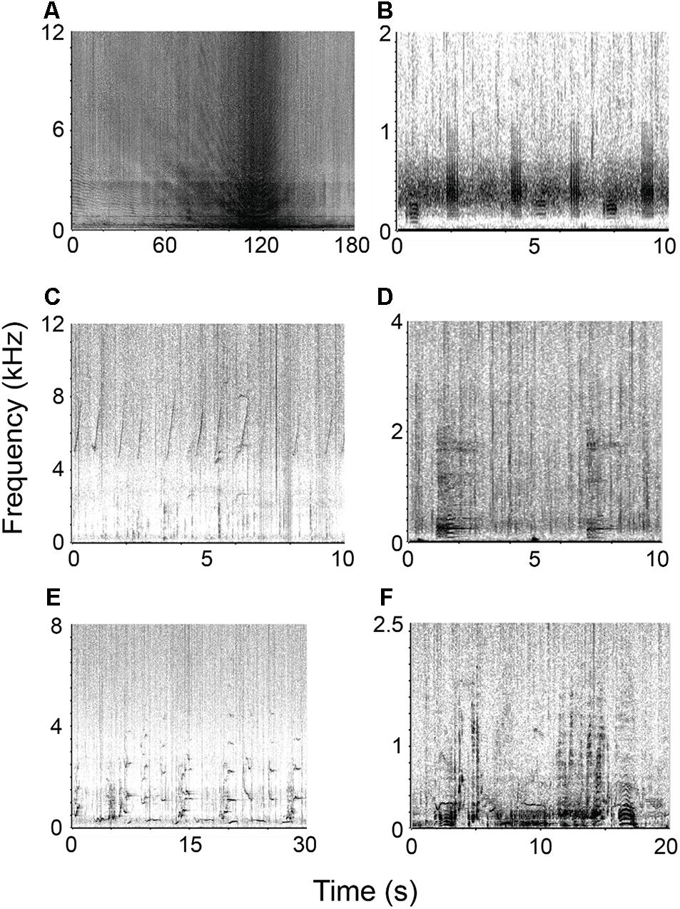
Figure 2. Representative spectrograms of various sound sources within the soundscapes of CGMP and SIMP. (A) close vessel passage, (B) fish chorusing, (C) dolphin whistles, (D) dwarf minke whale “star wars” call, (E) humpback whale song, and (F) humpback whale social calls.

FIGURE 3

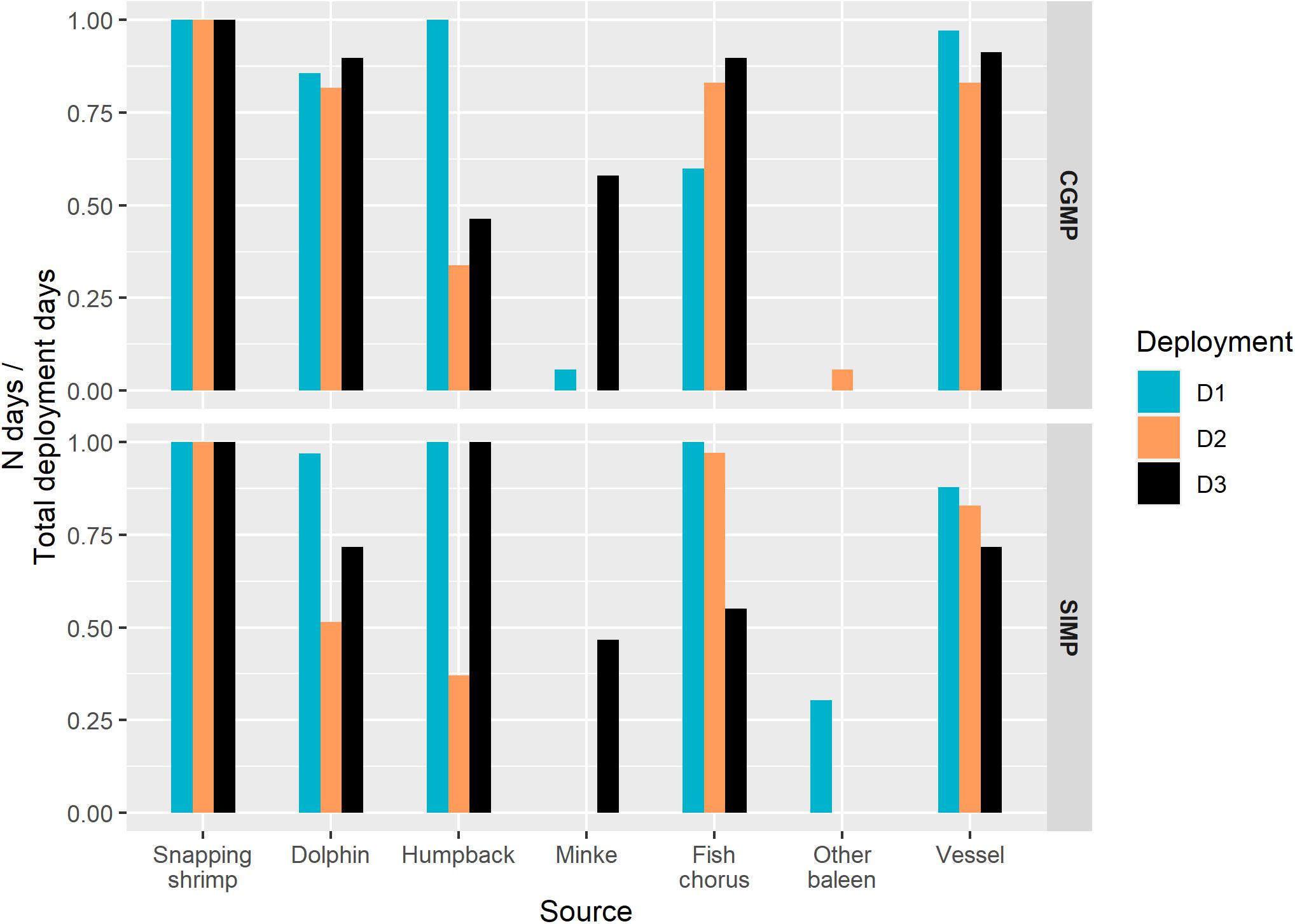
Figure 3. Seasonal presence of each sound source represented as the proportion of deployment days with at least 1 h present in Cod Grounds (CGMP, top) and Solitary Islands Marine Park (SIMP, bottom). Deployment is indicated by color and is used as a proxy for season (D1, D3 = austral winter; D2 = austral summer).

Biological Sound Sources

All six categories of biological sounds were present in the recordings. Two categories were able to be identified to species [humpback whales (Megaptera novaeangliae), dwarf minke whales (Balaenoptera acutorostrata)], while the remaining categories were identifiable to genus [snapping shrimp (Alpheus spp.)], family [dolphins (Delphinidae spp.)], or broader taxonomic categories (fish choruses, unidentified low-frequency baleen whales) (Figure 2).

Snapping shrimp, fish choruses, dolphins, and humpback whales were all present across all deployments (Figure 3). Minke whales were detected in CGMP D1, CGMP D3, and SIMP D3. Other baleen whales were detected in SIMP D1 and CGMP D2. Snapping shrimp were the most prevalent sound source in terms of daily presence and the only source present on 100% of days throughout all deployments. Fish choruses occurred on the majority of days in D1, D2, and D3 at both sites, although SIMP D3 showed a decrease in daily presence relative to other deployments (CGMP D1: 21/35 days, 60.00%; CGMP D2: 61/71 days, 85.92%; CGMP D3: 62/69 days, 89.86%; SIMP D1: 33/33 days, 100.00%; SIMP D2: 34/35 days, 97.14%; and SIMP D3: 33/60 days, 55.00%). Dolphins were present most days in all deployments, although D2 represented lower values for daily presence (CGMP D1: 30/35 days, 85.71%; CGMP D2: 58/71 days, 81.69%; CGMP D3: 62/69 days, 89.86%; SIMP D1: 32/33 days, 96.97%; SIMP D2: 18/35 days, 51.43%; and SIMP D3: 43/60 days, 71.67%).

For humpback whales, we detected instances of structured song at both sites in D1 and D3 as well as social calls in all deployments (Figure 3). In CGMP D1, SIMP D1, and SIMP D3, humpback song was present on all days. In CGMP D3, humpback whales were present on 32 of 69 days of the deployment (46.38%), and that deployment captured the onset of seasonal humpback whale song. The first instance of song was detected on May 16 and occurred on consecutive days from May 27 through the end of the deployment (June 24). In D2, humpback social sounds were detected intermittently at both sites (CGMP D2: 24/71 days, 33.80%; and SIMP D2: 13/35 days, 37.14%).

The dwarf minke whale “star wars” vocalization (Gedamke et al., 2001) was primarily present during D3 at both sites (Figures 2, 3). In CGMP D3, the call occurred on 40/69 days (57.97%) between April 27 and June 19 with the highest number of detected hours per day (N = 19 h) occurring on May 26 and May 31. In SIMP D3, the call was present for a total of 28/61 days (46.67%) between the first day of deployment (June 11) and July 11.

Low-frequency (<100 Hz) calls from other baleen whales were not able to be identified at the species level but based on comparison to the literature were most likely produced by either fin whales (Balaenoptera physalus) or blue whales (Balaenoptera musculus) (Širović et al., 2009; Erbe et al., 2017). These calls were detected on 4/71 days (5.63%) in CGMP D2 and on 10/33 days (30.30%) in SIMP D1.

Potential for Acoustic Niche Overlap

Daily presence was incorporated into spectral box display (SBD) plots to illustrate the potential for overlap in acoustic niche space on a daily and seasonal scale. Based on generalized frequency ranges for each source (Table 2), the SBD plots for all deployments show considerable overlap among sound sources in time and frequency (Figure 4). Most days throughout all deployments are represented by a combination of vessels and multiple biological sources. Snapping shrimp and dolphins dominate the higher frequency environment (>5 kHz), while fish choruses, humpback whales, and dwarf minke whales occupy the lower frequency bands within the typical frequency range of vessels from this study (95–3200 Hz). The temporal degree of overlap of humpback whales and dwarf minke whales with vessels largely depended on the deployment and followed the general pattern of seasonal presence in these species with more potential for overlap in D1 and D3.

TABLE 2

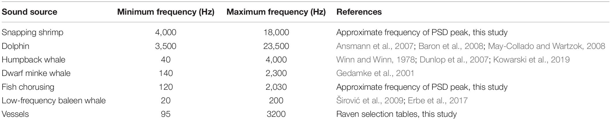
Table 2. Frequency ranges used to represent sound sources for SBD plots.

FIGURE 4

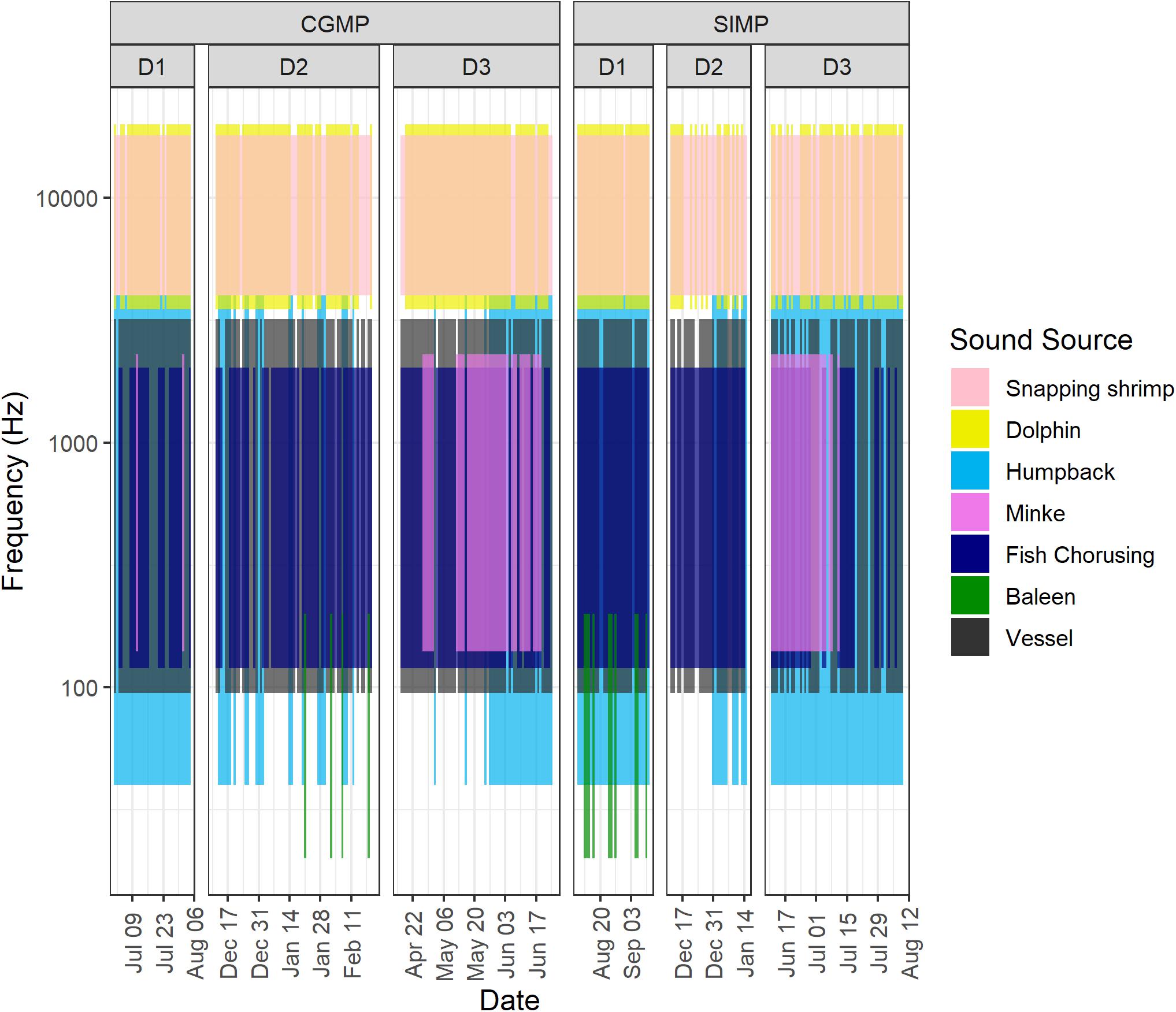
Figure 4. Spectral box display (SBD) plots for in Cod Grounds Marine Park (CGMP) (top) and Solitary Islands Marine Park National Park Zone (SIMP) (bottom). Vertical bars represent daily presence and approximate frequency range for each sound source indicated by color.

Diel Presence of Sound Sources

Anthropogenic Sources

Vessel presence showed a significant hourly difference among dawn, daylight, dusk, and night (Kruskal-Wallis test, p < 0.05) (Table 3). Pairwise comparisons showed that vessels had significantly higher presence in dawn and daylight hours compared to dusk and night hours (Dunn test: Z = 3.43–4.51, p_adj. < 0.05 for Dawn-Dusk, Daylight-Dusk, Dawn-Night, and Daylight-Night) (Figure 5).

TABLE 3

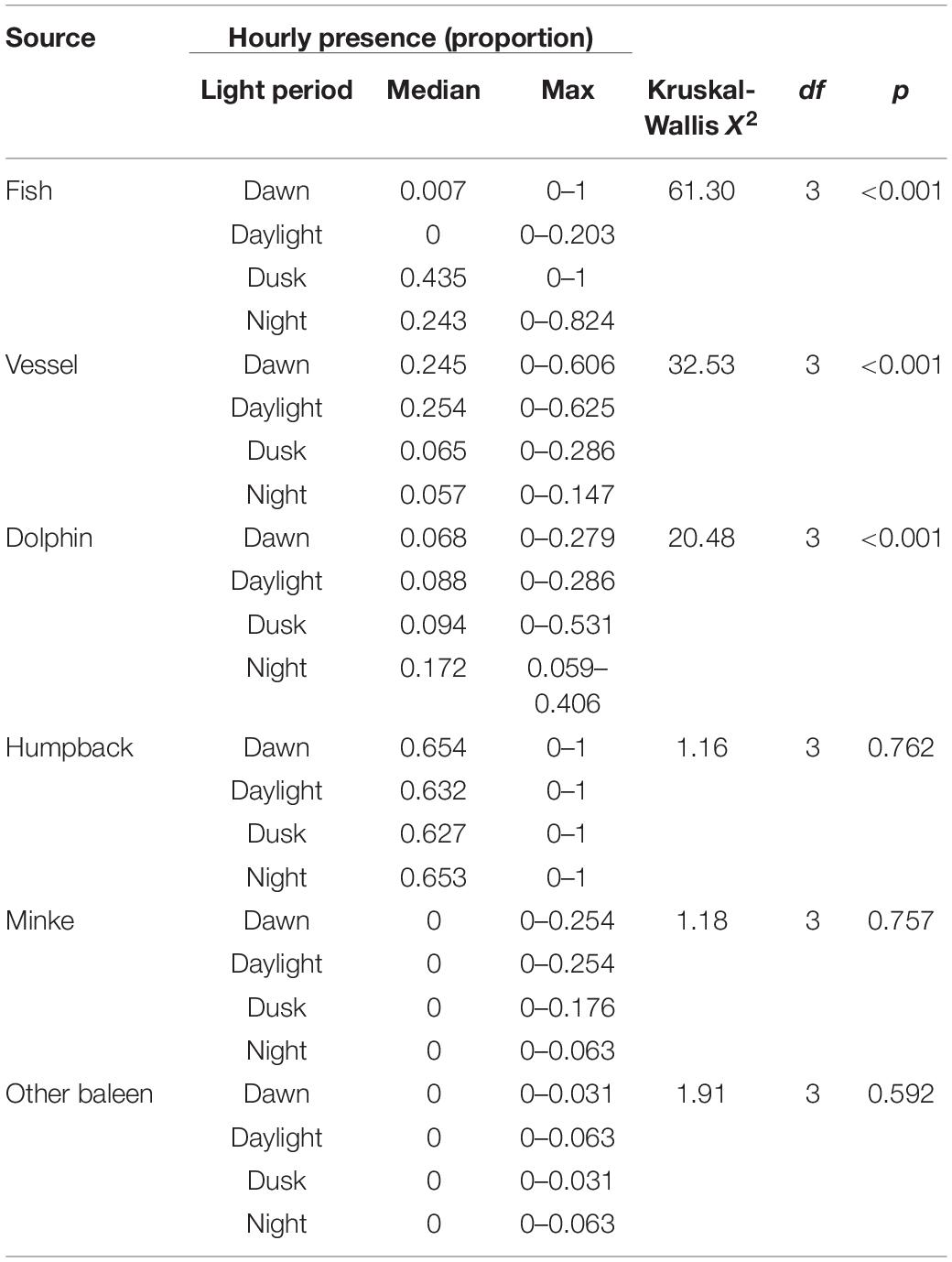
Table 3. Summary of overall Kruskall-Wallis tests for proportional hourly presence versus light regime.

FIGURE 5

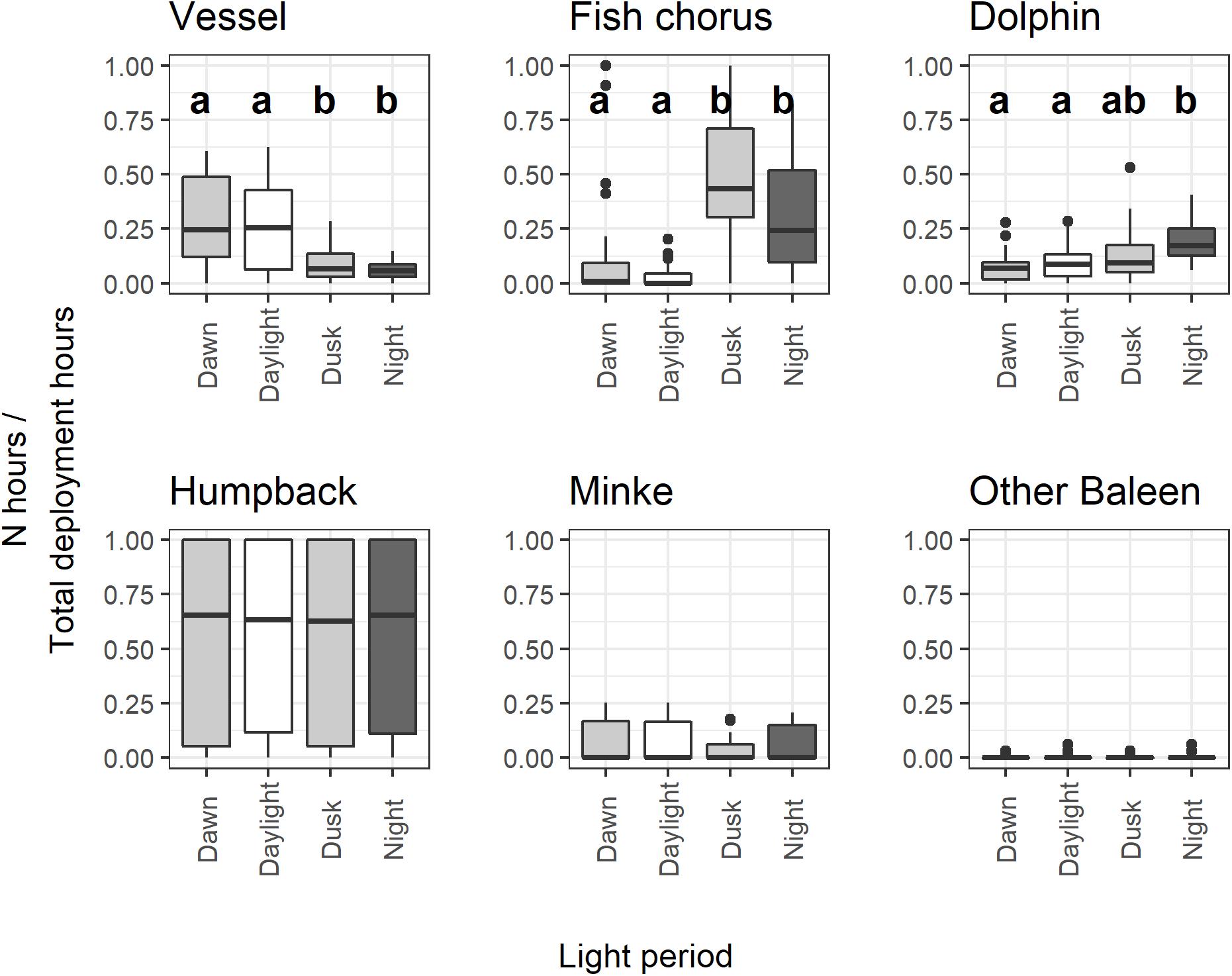
Figure 5. Boxplots of proportional hourly presence versus light regime pooled across all deployments. For sources with an overall significant effect of light regime (vessels, fish chorus, and dolphin; Kruskal-Wallis test, p < 0.05), different letters within each panel indicate light categories with significant differences according to post hoc examinations (Dunn test, p_adj. < 0.01 for all significant comparisons).

Biological Sources

Of the biological categories, fish choruses and dolphins had significant diel patterns in presence versus light regime (Kruskal-Wallis test, p < 0.05). Fish chorusing showed significantly higher presence in dusk and night hours (Dunn test: Z = -6.99– -2.96, p_adj. < 0.05 for Dawn-Dusk, Daylight-Dusk, Dawn-Night, and Daylight-Night) (Figure 5).

Weekly diel presence plots show that the evening chorus in all deployments occupies a larger range of times than the morning chorus (Figure 6). These plots also reveal differences between sites and seasons in fish chorusing behavior, such as the consistent timing of morning choruses in SIMP D1 and D2.

FIGURE 6

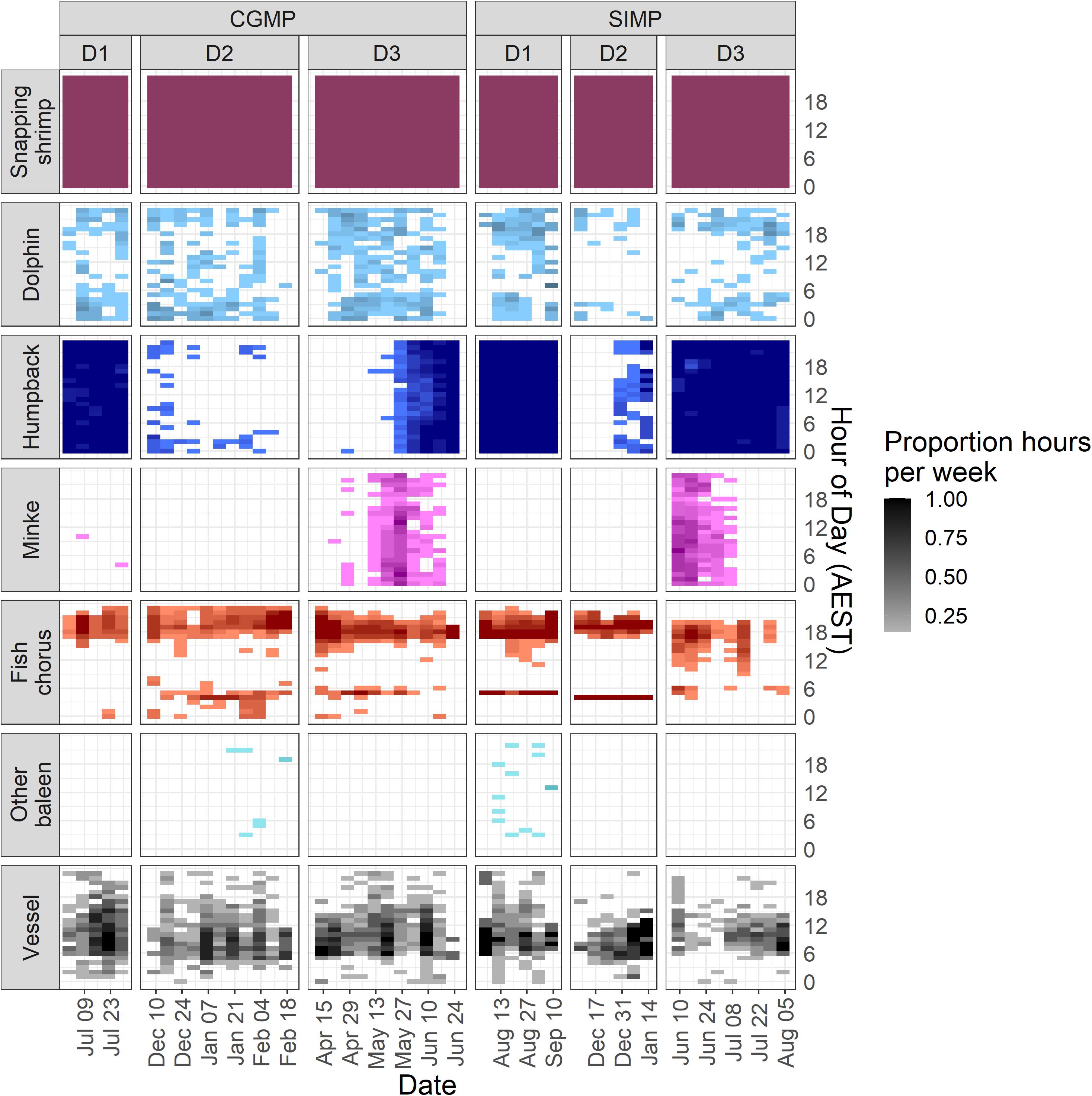
Figure 6. Hourly presence of each sound source aggregated by week in Cod Grounds Marine Park (CGMP) (left) and Solitary Islands Marine Park National Park Zone (SIMP) (right). Darker values represent more instances of a sound source being marked “present” during that hour in a given week (maximum = 7). White spaces indicate that sound source was not detected.

Dolphin presence at night was greater than all other categories and was significantly higher than dawn and daylight hours (Dunn test: Z = -4.14– -3.94, p_adj. < 0.05 for Dawn-Night, and Daylight-Night) (Figure 5). The dusk period was not significantly different from any of the other categories, suggesting this period had an intermediate level of dolphin presence. Weekly diel plots indicate dolphin presence was more evenly distributed throughout the day in CGMP than in SIMP, which was more apparent in SIMP D2 where there were no occurrences of dolphins between 06:00 and 12:00 (Figure 6).

Humpback whales, minke whales, and other unidentified baleen whales did not show a significant relationship with light regime (Kruskal-Wallis test, p > 0.05). Snapping shrimp were present during all hours of each deployment (Figure 6), which precluded statistical analyses of diel patterns in presence. Although diel patterns for shrimp could not be tested, review of the LTSA for all deployments showed a visible crepuscular pattern of increased amplitudes near dawn and dusk hours at frequencies consistent with snapping shrimp activity (Figures 7, 8).

FIGURE 7

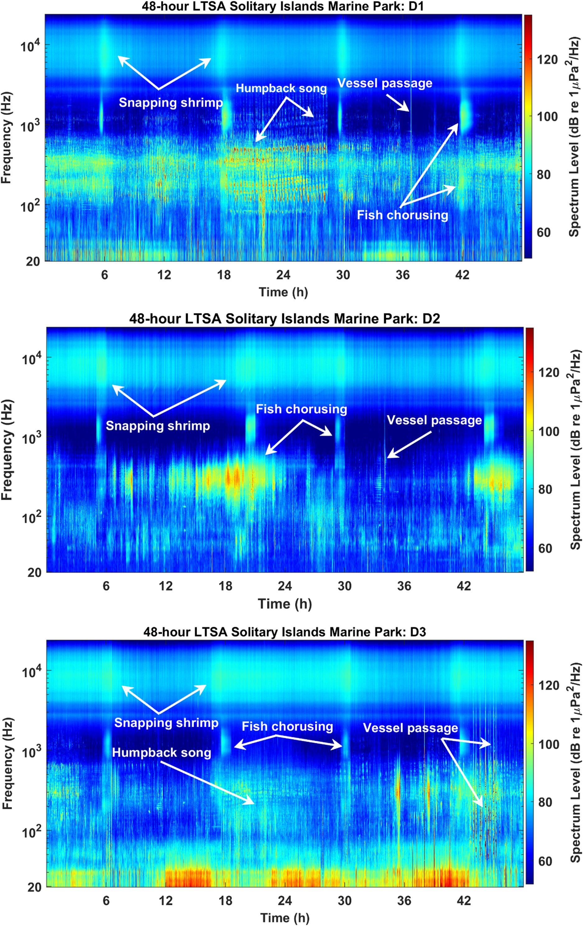
Figure 7. Example 48-h Long-Term Spectral Average (LTSA) plots for Solitary Islands Marine Park NPZ (SIMP) showing key sound sources in each deployment (top: D1, middle: D2, and bottom: D3). Plots were created using 1 Hz/1 min bins, and relative intensity of each bin is shown by the color scale.

FIGURE 8

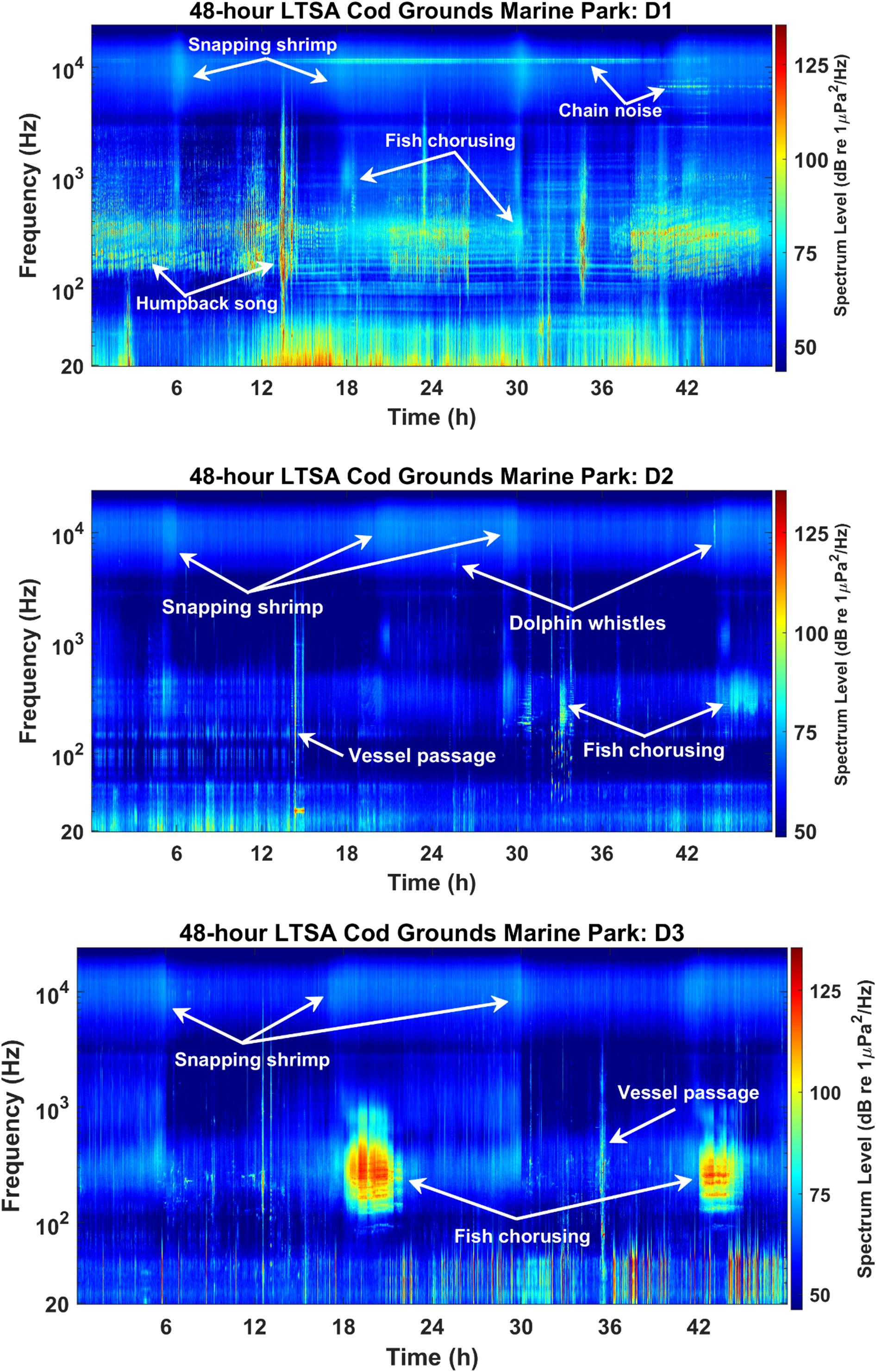
Figure 8. Example 48-h Long-Term Spectral Average (LTSA) plots for Cod Grounds Marine Park (CGMP) showing key sound sources in each deployment (top: D1, middle: D2, and bottom: D3). Plots were created using 1 Hz/1 min bins, and relative intensity of each bin is shown by the color scale.

Drivers of the Soundscape

Broadband Sound Pressure Levels (SPL)

Broadband sound pressure levels (SPL) showed a distinct diel pattern in all deployments with crepuscular peaks in the ambient sound levels (Figure 9). Of the sound sources showing statistically significant differences in presence across diel periods, the diel presence of fish choruses is most consistent with this pattern, particularly for dusk hours (Figures 6, 9). Snapping shrimp additionally showed a consistent diel pattern with increased crepuscular levels visible in the LTSA plots for all deployments (Figures 7, 8), and likely both sources are contributing to the overall diel pattern in SPL. Overall, the median broadband SPL in SIMP was higher than CGMP and more consistent across deployments, while in CGMP, the median broadband SPL was approximately 2 dB lower during D2 compared to D1 and D3 (Figure 9 and Table 4).

FIGURE 9

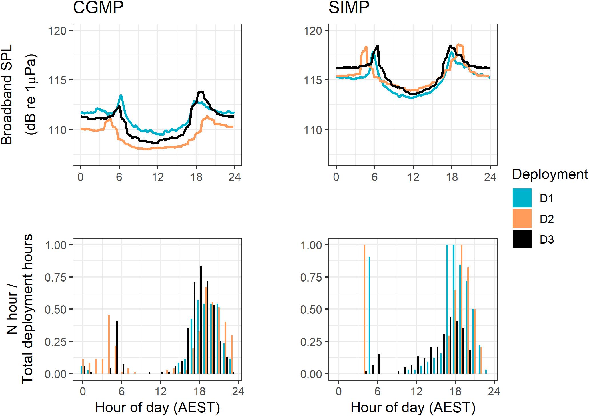
Figure 9. 5-min median broadband SPL levels (top row) and proportional hourly presence of fish choruses (bottom row) for all deployments in Cod Grounds Marine Park (CGMP, left column) and Solitary Islands Marine Park (SIMP, right column).

TABLE 4

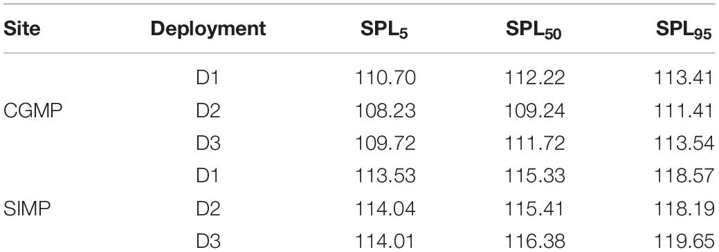
Table 4. Percentiles of broadband sound pressure level (SPL) measurements over each deployment.

Monthly Wind Observations

The proportion of wind observations occurring in the five wind speed categories significantly differed among all deployments (Coffs Harbour: X² = 624.81, df = 8, p < 0.01; Port Macquarie: X² = 174.51, df = 8, p < 0.01). Additionally, there were significant differences between all pairwise comparisons within each site (Table 5). Within each site, D2 had the highest proportion of wind speeds between 20–30 and 30 –40 kt. In Coffs Harbour, D2 additionally had the highest proportion of wind speed > 40kt (6.4%) compared to all deployments in both sites. In both sites, D3 had the highest proportion of wind speed observations between 0 –10 kt (Port Macquarie: 35.0%, Coffs Harbour: 31.5%). Overall, D1 represented intermediate wind conditions compared to D2 and D3 at both sites (Figure 10). When data were pooled across deployments to compare sites, sites were significantly different with Coffs Harbour having a lower proportion of observations between 0 and 10 kt (Coffs Harbour: 18.9%, Port Macquarie: 24.2%).

TABLE 5

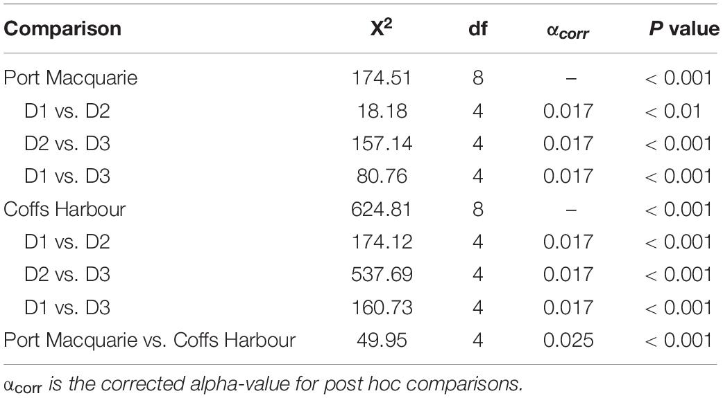
Table 5. Summary of Pearson’s Chi Square tests to compare wind conditions among deployments.

FIGURE 10

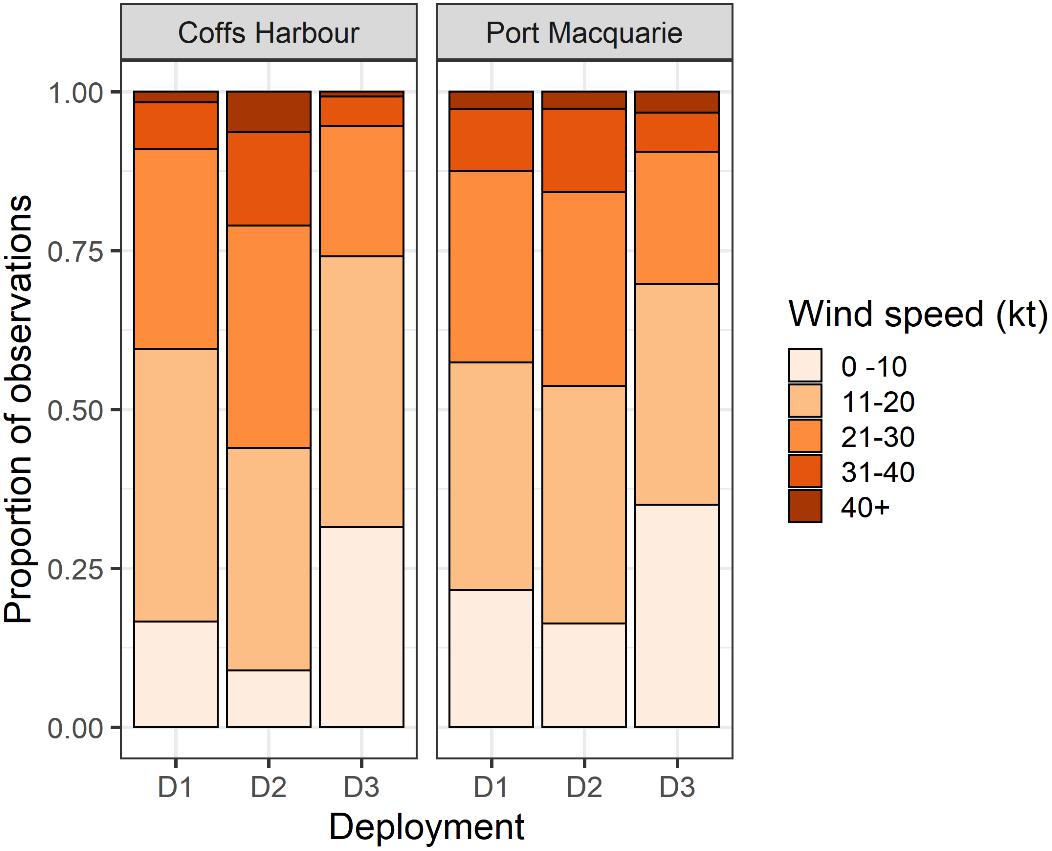
Figure 10. Proportion of historical wind observations over five categories of wind speed. Coffs Harbour is representative of the SIMP recording site, and Port Macquarie is representative of the CGMP site.

Power Spectral Density (PSD)

Across all deployments, the highest median PSD level occurred during SIMP D3 at 294 Hz (76.8 dB re 1 μPa²/Hz) (Figures 11, 12). Similar peaks in the median PSD were measured ∼300 Hz during D1 at both sites (CGMP: 310 Hz, 71.4 dB re 1 μPa²/Hz and SIMP: 331 Hz, 76.6 dB re 1 μPa²/Hz). This frequency is consistent with fish chorusing and humpback whale song during the winter deployments, suggesting these two sources are the primary contributors to the winter soundscape in both NPZs. During the summer deployments (D2), the ∼300 Hz peak in median PSD levels was absent, although a similar peak remained in the 95th percentile PSD levels, indicating a relatively loud source centered on that frequency but occurring less often than in the winter. This pattern further supports the strong influence of humpback whale song on the soundscape during the winter season as well as the influence of fish chorusing throughout all deployments. At both sites, there was a secondary peak in all plotted PSD levels between ∼4 kHz and ∼15 kHz, caused by snapping shrimp (CGMP: ∼10 kHz, 66.5 dB re 1 μPa²/Hz; SIMP: ∼8.8 kHz, 73.2 dB re 1 μPa ²/Hz). The relatively narrow range between the 5th and 95th percentiles at these frequencies indicates a more consistently loud source, which is additionally supported by our findings that snapping shrimp occurred in all hours throughout all recordings.

FIGURE 11

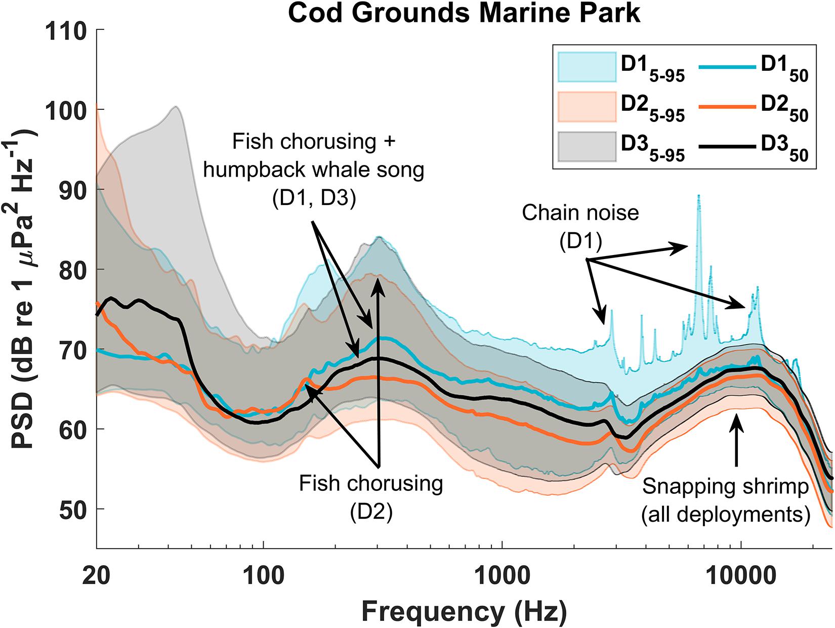
Figure 11. Power spectral density (PSD) plot for Cod Grounds Marine Park (CGMP). Relative peaks in the PSD values indicate higher acoustic energy in those frequencies over the entire deployment. Peaks were compared with Long-Term Spectral Average (LTSA) plots as well as with spectrograms from each deployment to identify the predominant contributors to each peak.

FIGURE 12

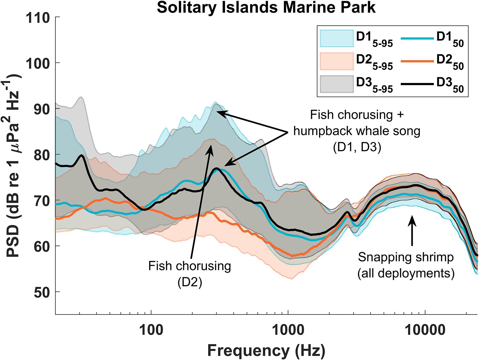
Figure 12. Power spectral density (PSD) plot for Solitary Islands Marine Park NPZ (SIMP). Relative peaks in the PSD values indicate higher acoustic energy in those frequencies over the entire deployment. Peaks were compared with Long-Term Spectral Average (LTSA) plots as well as with spectrograms from each deployment to identify the predominant contributors to each peak.

In CGMP D1, the rattling chain of a nearby mooring resulted in sharp peaks in the higher frequencies of the PSD (Figure 10), most notably in the 95th percentile curve but also visible in the median PSD levels. Additionally, stereotyped pulses ∼25-40 Hz in D3 at both sites contributed to a large peak in the 95th and 50th percentile PSD levels at those frequencies (Figures 10, 11). Although the source of the sound remains unknown, after comparison with known baleen whale and fish calls at similar frequencies, we concluded they are not likely to be biological in origin and hypothesize that these pulses may have been produced by some component of the recorder’s mooring.

Discussion

Soundscape metrics measured in CGMP and SIMP varied on both a seasonal and diel scale. Comparison with hourly presence of biological and anthropogenic sound sources indicated that these changes were primarily driven by biological sound sources—migratory humpback whale song on a seasonal scale and crepuscular reef chorusing of both fish and snapping shrimp on a diel scale. Seasonal differences in proportional wind speeds at weather stations closest to each site did not correspond to seasonal differences in SPL at either site. Anthropogenic sources were primarily represented by vessel passages which exhibited a significant diel pattern of higher presence during daylight hours but were not reflected in any soundscape metrics. These vessels did not appear to affect the long-term soundscape measurements in any deployment as their presence did not result in an identifiable increase in spectral levels.

Anthropogenic Sources

Review of spectrograms as well as LTSAs confirmed that while vessels were conspicuous, high-amplitude signals at short time scales—particularly closer passages with energy above ∼2 kHz—at the scale of several hours to days they did not comprise a prominent, identifiable component of the soundscape. Vessel signatures did not contribute to peaks in either the PSD or SPL measurements from any deployment. Since vessels represent a broadband signal, they may be less likely to form identifiable peaks in the PSD plots and may instead contribute to overall noise levels across frequencies. It is important to note, however, that vessels were present on the majority of days during each deployment and still contribute to the anthropogenic noise within both NPZs. While vessel noise may not be as pervasive as biological sound sources at these sites on the scale of weeks to months, it should not be ignored by managers as an anthropogenic threat within the NPZ. Effects of vessel-generated noise on the species within these NPZs could include masking of communication signals, habitat abandonment, decreased larval recruitment to reefs, and physical damage to hearing structures (e.g., Piercy et al., 2014; Harris et al., 2018; Duarte et al., 2021). The SBD plots additionally indicate potential for these effects due to the temporal and frequency overlap of vessels with multiple biological sources. Further study of the spatial distribution of both anthropogenic and biological sources would be valuable in determining the extent of specific impacts of noise within these MPAs.

From a management perspective, it is promising that although vessels are prevalent during daylight hours, they do not seem to be altering the diel ambient levels of the soundscape (i.e., SPL) at the scale of an entire deployment, further supported by the result that vessel hourly presence was significantly higher during daylight hours represented by lower SPL values. Based on available AIS data (Lucieer et al., 2017; Peel et al., 2019), both marine parks are situated near areas of concentrated shipping traffic, with a higher-density shipping channel near CGMP (approximately 1–3 nautical miles to the closer edge of the channel) compared to a slightly farther, lower-density shipping channel near SIMP (approximately 5–8 nautical miles to the closer edge of the channel). Due in part to their location near the coast, both NPZs additionally fall within a marine acoustic zone predicted to be more heavily influenced by anthropogenic sound sources than weather and wind-driven sound sources (Erbe et al., 2021a, b). Our analysis of proportional wind speeds further supports the conclusion that geophony resulting from wind at these sites is not a major driver of seasonal changes in the soundscape metrics. Several factors including vessel size, speed, and distance to recorder (National Resource Council, 2003) affect the degree to which vessel traffic influences a soundscape at different time scales. Large vessels in particular are known to have higher source levels than small vessels (e.g., recreational vessels) and are thus more likely to influence measurements of a soundscape (National Resource Council, 2003). Kline et al. (2020) found that the majority of vessels in these NPZs were likely to be small or medium vessels transiting outside of the NPZ boundaries, and the paucity of close passages from large vessels may explain the discrepancy between the persistent presence of detected vessels and their apparent absence as an important contributor to the overall soundscape characteristics. Anthropogenic sources occurring beyond the boundaries of protected areas often still affect soundscapes within those boundaries (e.g., Hatch and Fristrup, 2009; Buscaino et al., 2016; Pavan, 2017; Haver et al., 2020). This is especially pertinent for smaller MPAs such as SIMP and CGMP where the detection range of large vessels is greater than the distance from the recorder to the park boundary (Kline et al., 2020), further complicating the task of managing MPAs toward soundscape conservation.

Biological Sources

Although anthropogenic noise from vessels represents a potentially disruptive signal capable of effects ranging from acoustic masking to physiological stress (Brumm and Slabbekoorn, 2005; Rolland et al., 2012; Blair et al., 2016), many marine soundscapes show changes driven by biological sound sources rather than anthropogenic noise [e.g., Adriatic Sea (Pieretti et al., 2017); North Sea (Putland et al., 2017); Glacier Bay, Alaska (Fournet et al., 2018; Haver et al., 2019); American Samoa and U.S. Virgin Islands (Haver et al., 2019)]. Both NPZs in this study showed increased median PSD levels between ∼100 and 2000 Hz during the winter deployments compared to the summer deployments. Comparing this increase in acoustic levels with hourly presence of sound sources, the change is most consistent with the presence of migratory humpback whales and dwarf minke whales during the winter season. The seasonal presence for both species follows the timing of the northward migration from summer feeding grounds (Brown et al., 1995; Gedamke et al., 2001; Dunlop et al., 2008), and the presence of humpback social sounds in the summer deployments suggests they may use these temperate areas outside of the regular reproductive and migratory seasons. Although vessels and fish choruses occupy a similar frequency range (Table 2), neither of those sound sources showed major differences in presence across seasons and were unlikely to be the primary cause of the higher SPL values in D1 and D3. The presence of seasonal reproductive displays such as harbor seal roars (Fournet et al., 2018; Haver et al., 2019) and humpback song (Haver et al., 2019; Kügler et al., 2020) has been shown elsewhere to dramatically alter seasonal ambient sound levels.

On a diel scale, dolphins showed a pattern of significantly higher hourly presence during night hours, potentially related to increased foraging or socializing at these times (Gregorietti et al., 2021). The increased nocturnal activity of dolphins was not apparent in SPL or PSD metrics, likely due to the short duration and transient nature of calling events. Humpback whale songs and social calls did not show significant diel patterns in hourly presence although humpback whales in other locations have been shown to increase singing activity at night (Kobayashi et al., 2021). However, the general pattern of the diel SPL values remained consistent across seasons, suggesting that any nocturnal increases in singing activity at these NPZs were not pervasive enough to affect diel patterns of SPL measurements during the winter deployments.

Both sites exhibited crepuscular peaks in SPL consistent with a typical reef chorus of fish and snapping shrimp (Cato, 1978; McCauley, 2012; Buscaino et al., 2016; Dimoff et al., 2021). Examination of LTSA plots revealed a distinct crepuscular pattern of increased amplitude between ∼4 and 18 kHz, consistent with snapping shrimp behavior in other soundscapes (Pieretti et al., 2017). Given that the crepuscular SPL peaks occurred in all deployments despite a lack of consistent morning fish choruses in some deployments, snapping shrimp may represent the primary source of diel variation in broadband SPL values. In CGMP, a peak ∼150Hz in the median PSD corresponded with peak frequencies of observed fish choruses. In SIMP, peaks in the 95th percentile PSD near 200 Hz corresponded with fish chorus frequencies in all deployments, but the median PSD levels did not show any prominent peaks during the summer deployment. Fish choruses in SIMP were generally shorter and more consistently timed than in CGMP (Figures 6, 9); this less frequent signal may be more likely to influence a peak in the 95th percentile but not the median (50th) percentile PSD levels (Figure 11). In SIMP, the SPL was generally higher than CGMP and less variable across seasons (Figure 9). The overall difference in SPL between the sites may reflect a higher relative abundance of acoustically active species within SIMP overall or closer proximity of the recorder to a complex, hard reef substrate which may represent a higher local concentration of such species (e.g., Freeman and Freeman, 2016; Rossi et al., 2016).

SBD plots show that despite overlap in daily acoustic niche space, both sites show a similarly complex, diverse acoustic community with considerable frequency overlap among multiple biological categories. On a diel scale, however, sources vary in presence patterns, ranging from nearly continuous seasonal presence (e.g., humpback whales) to consistent crepuscular patterns (e.g., snapping shrimp and fish choruses). Further studies could build upon these baseline assessments and determine whether fine-scale temporal acoustic partitioning occurs among biological sources in these soundscapes. For example, humpback whales have been shown to reduce rates of foraging and social calls in the presence of both biological and anthropogenic sounds (Blair et al., 2016; Fournet et al., 2018), potentially representing a compensation strategy via temporal partitioning of acoustic space (Krause and Farina, 2016). Vessel presence has also been shown to reduce singing activity of humpback whales in other areas (Sousa-Lima and Clark, 2008), although further work would be required to determine whether such a reduction would be detectable at the level of the soundscape measurements analyzed in this study.

Management Implications

Soundscape metrics such as SPL and PSD provide an efficient means of assessing the presence of various sound sources within an area. However, soundscape ecology by definition focuses on large-scale patterns of the soundscape rather than a detailed analysis of the characteristics of each sound source (Pijanowski et al., 2011). The present study does not, therefore, address detailed aspects of certain acoustic contributors as is more typical of traditional bioacoustics research—e.g., species-level identification of fish choruses, snap rates of snapping shrimp, specific call types of humpback whale song or social calls. Although such measurements are valuable and would contribute to a deeper understanding of acoustic interactions at a finer scale, they were not possible within the scope of this study.

Conserving biodiversity within MPAs requires knowledge of existing conditions to determine efficacy of management decisions, and the baseline measurements presented here ideally would be further expanded with future monitoring efforts. Although each deployment in this study lasted over a month, additional deployments would allow both a comprehensive analysis of year-round changes in the soundscape as well as provide multiple representative examples of soundscape characteristics for each season. Since the baseline conditions presented here represent temporal changes at a single location in each NPZ, any future deployments should occur in the same location to facilitate comparison to these data. Despite the small size of these NPZs, it is possible that the soundscape would exhibit spatial heterogeneity resulting from small-scale differences in bathymetric features, vessel activity, or density of calling species.

Concurrent surveys to confirm species of dolphins or chorusing fish would provide additional ground-truthing of species-specific effects on measurements of the soundscape. Such ground-truthing could enable managers to use relevant changes in PSD or SPL values as a proxy for trends in abundance of those species within the NPZs (Freeman and Freeman, 2016; Coquereau et al., 2017; Kügler et al., 2020). If soundscape measurements can be used to detect changes in acoustic presence of individual species, this method could expedite monitoring efforts compared to manually reviewing vocalizations: a method which is thorough yet time intensive. When monitoring the soundscapes of MPAs, managers must consider the underlying patterns of change within the soundscapes before assessing impacts due to anthropogenic influence. For example, based on this study, changes in the relative contribution of anthropogenic sound sources may be more easily detected using ambient sound metrics taken from summer recordings to avoid confounding effects from humpback whale song.

We found that vessel noise was not a major contributor to the long-term soundscape metrics of either NPZ; however, we recommend that managers continue monitoring vessel use within the NPZs to assess trends in relative contributions from biological and anthropogenic sources. Although vessels were detected via manual review in this study, future efforts could incorporate automated or semi-automated detectors to assess presence of sound sources and improve standardization of metrics across multiple soundscapes (e.g., Ainslie et al., 2018). The underwater soundscapes of MPAs can show high variation over time and space (Haver et al., 2019), and using standardized metrics enables efficient and informative comparisons of soundscape characteristics (Merchant et al., 2015). Consistent recording efforts can additionally provide opportunities to study effects of unforeseen events that may affect anthropogenic activity, such as the reduction in shipping traffic and associated noise levels following the events of September 11, 2001 (Rolland et al., 2012) or recent COVID-19 confinement strategies (Thomson and Barclay, 2020). Long-term comparative studies of soundscapes within MPAs could provide managers with early indications of disturbance due to threats including climate change and increased anthropogenic noise levels (Halpern et al., 2015; Krause and Farina, 2016; Rossi et al., 2016; Coquereau et al., 2017).

Data Availability Statement

The raw data supporting the conclusions of this article will be made available by the authors, without undue reservation.

Ethics Statement

Ethical review and approval was not required for the animal study because this study was conducted entirely using passive remote monitoring techniques that did not involve any interactions between researchers and animals.

Author Contributions

JM, SV, JSt, and AD contributed to conception and design of the study. JSm, GR, and CM provided institutional and logistical support for fieldwork and data transfer. JM, LK, and AS completed data processing. JM completed analyses with assistance from AD, TR, and JSt. JM wrote the initial draft of the manuscript. All authors read and approved the submitted version.

Funding

This research was funded by the Director of National Parks, Australia.

Conflict of Interest

JM was employed by company Integrated Statistics, Inc.

The remaining authors declare that the research was conducted in the absence of any commercial or financial relationships that could be construed as a potential conflict of interest.

Publisher’s Note

All claims expressed in this article are solely those of the authors and do not necessarily represent those of their affiliated organizations, or those of the publisher, the editors and the reviewers. Any product that may be evaluated in this article, or claim that may be made by its manufacturer, is not guaranteed or endorsed by the publisher.

Acknowledgments

The authors would like to thank the New South Wales Department of Primary Industries staff at Coffs Harbour and Port Macquarie for their assistance in the deployment and retrieval of acoustic recorders. The authors would also like to thank Genevieve Davis for providing valuable assistance with figures as well as three reviewers for comments that greatly improved the manuscript.

References

Ainslie, M. A., Miksis-Olds, J. L., Martin, B., Heaney, K., de Jong, C. A. F., von Benda-Beckmann, A. M., et al. (2018). Underwater Soundscape and Modeling Metadata Standard. Technical Report by JASCO Applied Sciences for ADEON Prime Contract No. M16PC00003). Durham, NH: University of Hampshire.

Google Scholar

Ansmann, I. C., Goold, J. C., Evans, P. G. H., Simmonds, M., and Keith, S. G. (2007). Variation in the whistle characteristics of short-beaked common dolphins, Delphinus delphis, at two locations around the British Isles. J. Mar. Biol. Assoc. UK 87, 19–26. doi: 10.1017/S0025315407054963