The Identification and Prediction in Abundance Variation of Atlantic Cod via Long Short-Term Memory With Periodicity, Time–Frequency Co-movement, and Lead-Lag Effect Across Sea Surface Temperature, Sea Surface Salinity, Catches, and Prey Biomass From 1919 to 2016

The population of Atlantic cod significantly contributes to the prosperity of fishery production in the world. In this paper, we quantitatively investigate the global abundance variation in Atlantic cod from 1919 to 2016, in favor of spatiotemporal interactions over manifold impact factors at local observation sites, and propose to explore the predictive mechanism with the help of its periodicity, time–frequency co-movement, and lead-lag effects, via long short-term memory (LSTM). We first integrate evidences yielded from wavelet coefficients, to suggest that the abundance variation potentially follows a 36-year major cycle and 24-year secondary cycle at the time scales of 55 years and 37 years. We further evaluate the responses of Atlantic cod abundance to the external impact factors, including sea surface temperature (SST), catches, prey biomass, and sea surface salinity (SSS), in aid of the wavelet coherence and phase difference, which allows us to identify the dominantly correlative factors and capture the leading roles along the time domain and then divide the responses around the recent 60 years into three stages: before 1985, 1985–1995, and after 1995. At the first stage, the reason for the decline in abundance could be mainly attributed to the rapid rise of fish catches. At the second stage, the impact of SST and SSS also provides significant indices, besides overfishing; meanwhile, the mortality of primary producers and forced migration of fish species indirectly cause the decline. At the third stage, warming SST and growing SSS directly led to the decrease of abundance. Finally, we establish one ensemble of LSTM-SAE architecture to comprehensively reflect the predictive patterns at each stage. It has been demonstrated from experimental results that the models behaved better when intentionally feeding with the dominantly correlative multivariate inputs, instead of either all factors or only the abundance. The proposed scheme provides opportunities to symmetrically identify the underlying predictive attributes of Atlantic cod abundance and potentially perform as the quantitative references in reasonably making fishing decision. With the rapid development in deep learning capabilities, it is hopeful to expect better predictions of the responses to global changes, not only for Atlantic cod but also for other fish species and the ecosystem as a whole.

Introduction

Atlantic cod (Gadus morhua), one of the most consumed edible fish species with great economic values, is fecund with reproductive potentials, but has long been overfished and highly associated with marine environment changes, causing dramatic declines for decades. The symmetrical investigation on the known abundance variability in Atlantic cod could integrate evidences on its spatiotemporal responses to manifold intrinsic and external indices and help provide opportunities to explore the underlying patterns and mechanism of Atlantic cod abundance to be predicted.

There might exist quite a few possible reasons behind the abundance variation of Atlantic cod, in combination with the life history characteristics (Jordaan, 2002; Drinkwater, 2005; Kristiansen et al., 2011; Árnason et al., 2013). First of all, from the perspective of marine ecology, the adaptability of Atlantic cod in both the early stage of life and adulthood depends much on the food supply and seawater temperature (Rose and Leggett, 1989; Miller et al., 1995). Sea surface temperature (SST) behaves as one of the most essential and fundamental indices (Fullard et al., 2000; O’Brien et al., 2000; Pörtner et al., 2001), indirectly delivering influences to the physical and biological systems of the deeper ocean for the benthic Atlantic cod habitat (Parmesan and Yohe, 2003; Rao and Sivakumar, 2003; Rosenzweig et al., 2008), altering both benthic and pelagic ecosystems from phytoplankton to zooplankton to higher trophic levels (Meyer et al., 1999; Richardson and Schoeman, 2004; Wanless et al., 2005; Behrenfeld et al., 2006). SST dictates movement and habitat connectivity of Atlantic cod (Staveley et al., 2019). Warming sea temperature causes Atlantic cod to move out of the habitat, either entering deeper waters or migrating to more northerly waters. The higher sea temperature also brings huge varieties in the number of primary producers, as well as their seasonal growth changes, which will definitely disrupt the normal food supply and nutrition that feed Atlantic cod (Schwalme and Chouinard, 1999; Drinkwater et al., 2000). Atlantic cod’s diet ranges from phytoplankton and small zooplankton as the larvae, to crustaceans and shrimps when they gradually grow up after the larval stage, to capelin, sand lance, herring, red fish, etc., and even other cod (Scott and Scott, 1988; Bogstad et al., 1994; Sundby, 2000), where the structure or abundance modification of the primary nutrition may propagate through higher trophic levels at the basis (Kirby and Beaugrand, 2009).

Meanwhile, ocean acidification driven by rising global CO₂ concentrations increases the sensitivity of Atlantic cod embryos to extreme temperatures, which results in tissue damage to cod larvae and changes in their behavior (Dahlke et al., 2017; Sswat, 2017); the decrease of seawater salinity inhibits the activity of sodium and potassium ions and decreases plasma osmotic pressure, influencing the feeding conditions of Atlantic cod, resulting in decreased recruitment (Lambert et al., 1994; Conover et al., 1995; Beaugrand et al., 2011). In addition, ocean currents, with their vertical or horizontal movement of both surface and deep water throughout the ocean, are also considered to contribute to the propagation and redistribution of marine thermocline and marine nutrients during the growth of Atlantic cod (Wroblewski et al., 2000; Hays, 2017). It is also argued that the rapid development of fishing technology from the 1980s has played a major role in the collapse of the Atlantic cod abundance in the North Atlantic (Baird et al., 1991; Hutchings and Myers, 1994; Hutchings, 1996). Although a series of restricted fishing and even fishing bans have been issued since 1992, the scale of local Atlantic cod like Canada has not shown significant signs of rebound (Myers et al., 1997). The variation of Atlantic cod abundance is undoubtedly not determined by a single impact factor but attributed to the outcome systemically and integrally generated from the series of intrinsic and extrinsic relevant indices that directly or indirectly interact with the abundance from the perspective of environment, physiology, migration, reproduction, and so on.

The relationship between Atlantic cod abundance and manifold impact factors is always not a simple causal function. It has been noted that most commonly applied approaches, such as bootstrapping regression models (Freedman, 1981), rolling window regression (Oehlert and Swart, 2019), and auto-regressive distributed lag (ADL) model (Haseeb et al., 2019), often only consider one single or several independent predictive elements and tend to ignore the combined effects of the complex marine climates and ecosystem structures, which is too idealized, while the classic correlation calculation is only suitable for studying relatively short-term time series and severely limited to stationary series. Therefore, on the basis of the historic spatiotemporal responses to manifold intrinsic and external indices, how to establish a comprehensive predictive framework that potentially explores underlying mechanism for its variation of Atlantic cod abundance is actually a pioneering topic. Firstly, the abundance variation in Atlantic cod may inherently follow its own specific patterns that probably present elementary periodic tendencies or illustrate some time–frequency characteristics (Berberidis et al., 2002). Secondly, no matter the time series of Atlantic cod abundance itself or the extrinsic correlative indices in study, most of them are non-stationary for a quite long period, where the possible mutations may occur in any individual stage, so that there may be time–frequency co-movements at a specific moment or relatively short period (Vacha and Barunik, 2012). Finally, there exist lead-lag effects diversified between Atlantic cod abundance and manifold impact factors, indicating a variety of modifications in the leading roles that will dominate co-movements in every certain time period, at a certain influencing direction of either positive or negative correlation (Dajcman, 2013).

To address the potential periodicity, time–frequency co-movement, and lead-lag effects of non-stationary long-term time series, wavelet analysis is a mathematically basic tool to discover how to approximate time series to a certain frequency band within a certain time period simultaneously, which could optimally describe the occurrence of transient events, and well adapt to conditions where the amplitude of the response varies significantly in non-stationary time series (Steel and Lange, 2007; Cloern and Jassby, 2010; Rhif et al., 2019). As the extended usage of wavelet transform, wavelet coherence (Maraun and Kurths, 2004; Su et al., 2018, 2019) and phase difference (Aguiar-Conraria and Soares, 2011) can be utilized to recognize whether two time series are quantitatively linked by a certain correlation, even causality relationship. Kogovšek et al. (2010) have applied continuous wavelet transform to investigate the long-term fluctuation of time series of jellyfish abundance in the past 200 years and further confirmed a major and minor period of its proliferation. Carey et al. (2016) adopted continuous wavelet transform to identify the periodic changes of phytoplankton at multiple time scales and determined the dominant scale of its periodic changes. Ménard et al. (2007) has quantified the non-stationary association between the Indian Ocean climate and tuna populations through wavelet analysis and further explored the dependency between them. Li et al. (2015) have adopted wavelet analysis to explore the multi-temporal scale characteristics and interrelationships between algal biomass and selected aquatic environmental parameters and tried to explain the complex non-linear eutrophication dynamics. All of the above wide range of applications reflect to varying degrees the efficacy of wavelet analysis in non-stationary long-term multivariate time series at multiple time scales.

In addition, in order to comprehensively investigate the mutual influences between manifold intrinsic and external indices, we tried to develop multivariate prediction model for the variation tendency of Atlantic cod abundance in a longer-term move. Traditional time series prediction methods, like hidden Markov model (HMM) (Rabiner and Juang, 1986), Auto-regressive integrated moving average (ARIMA) (Zhang, 2003), moving average model (MA) (Box and Pierce, 1970), etc., often have a complicated modeling process, and when it comes to multi-step forward prediction problem, most of them do not have ideally consistent performances in the long run. For decades, machine learning (ML) has become one of the most powerful tools in the field of multivariate multi-step time series prediction (Joy and Death, 2004; Yáñez et al., 2010; Miller et al., 2019), while deep learning can be regarded as one of the hottest topics developed recently in the context, which drives predominant forces in modeling, functioning, forecasting the structural, long-term, dynamic properties in time series, and all kinds of most emerging and advanced algorithms have been put forward and made progresses (Hinton and Salakhutdinov, 2006; Krizhevsky et al., 2012; Huang et al., 2017).

Among them, the deep architecture of the recurrent neural network (RNN), which could model the sequences at the arbitrary length by applying a transition function to all its hidden layer states in a recursive manner, and capture all information stored in sequence in the previous element (Jagannatha and Yu, 2016; Fan et al., 2017), has been proven to be superior in prediction. Long short-term memory (LSTM) has been revolutionarily designed by adjusting the structure of the hidden neurons in RNN, based on a series of memory cells recurrently connected through layers to capture and retain the long-term dependencies, not only suppressing the disappearing gradient problem, but also enhancing the capability in predicting multi-step ahead into the future (Duan et al., 2016; Zhang et al., 2017; Park et al., 2018).

Despite the fact that LSTM models have outstanding advantages in prediction accuracy, its performance remains unsatisfactory, particularly when attempting to process highly non-linear and long-interval time series. There are hereby quite a lot of variant LSTM algorithms newly developed, including bidirectional LSTM (Bi-LSTM) (Habernal and Gurevych, 2016), gated recurrent unit (GRU) (Dey and Salem, 2017), LSTM-based stacked autoencoder (LSTM-SAE) (Sagheer and Kotb, 2019), etc. Among them, LSTM-SAE improves the random initialization strategies in an unsupervised learning fashion and circumvents the expression limitations of the conventional shallow LSTM model, which could hereby, to some extent, alleviate the convergence to local minimum and perform better in multi-step prediction.

In this article, in order to explore the potential response mechanism of Atlantic cod abundance changes, we make an attempt to establish a comprehensive prediction model of Atlantic cod abundance, with the help of its periodicity, time–frequency co-movement, and lead-lag effects, which can quantify spatiotemporal interactions with manifold intrinsic and external indices. We systematically retrieve the annual abundance of Atlantic cod, the catches, the biomass of primary producers, SST, and sea surface salinity (SSS), respectively, from BioTIME, FAOSTAT, ERSST.v5, and EN4, and select local observation sites with relatively complete abundance records for our study, i.e., ID 119 near the Gulf of Maine and ID 428 on the southeastern coast of Norway, to accordingly attain standardized time series at specific geographical coordinates, by spatial and time averaging. We employ the modulus and variance of wavelet coefficients to reveal the potential periodicity of global Atlantic cod abundance, to generate the wavelet coherence map by the ratio between the wavelet cross-spectrum and power spectrum, to evaluate the responses of the abundance variability toward the external impact factors, and to produce the wavelet phase difference by the ratio between the imaginary and the real part of the wavelet cross-spectrum, to reflect leading roles that dominate time–frequency co-movements in every certain time period. This will provide a complete framework for the quantitative correlation and even causality among multivariate time series at multiple stages. Finally, in view of the historical time–frequency responses between Atlantic cod abundance and manifold impact factors, we attempt to determine the comprehensive prediction patterns of Atlantic cod abundance, by establishing the ensemble of LSTM-SAE architecture at each stage, and respectively, feed into three types of input vectors, namely, Atlantic cod abundance itself, all the external impact factors, and the dominantly correlative impact factors, to help with the estimation.

The remainder of the paper is organized as follows: Section “Materials and Methods” describes the access of multivariate time series referred, and outlines the basics in periodicity, wavelet coherence, phase difference, as well as the LSTM-SAE architecture in our study. Section “Results” quantitatively and systematically investigates the periodicity, time-frequency co-movement, and lead-lag effects in abundance variation of Atlantic cod, regarding the external impact factors, SST, catches, prey biomass, SSS, and exhibits the experimental results. Section “Discussion” suggests potentially mutual relationships along the time domain, together with the known events and its consequences, divides the responses of Atlantic cod abundance into stages, and establishes the ensemble of LSTM-SAE architecture for multivariate prediction. Finally, the conclusions are drawn in Section “Conclusion”.

Materials and Methods

Data

Atlantic Cod Abundance

The abundance of Atlantic cod has been retrieved via BioTIME database, which is composed of more than 12 million records of the raw data on species identities and abundances in ecological assemblages of more than 20 biomes at 361 observation sites from 1858 to 2018, where 5,640,610 records collected from six communities have been applied here from fish to marine invertebrates, consisting of the most comprehensive database for marine species abundance and richness statistics. Atlantic cod mainly inhabit most waters overlying the continental shelves of the Northwest and the Northeast Atlantic Ocean, such as the Gulf of St. Lawrence (Lambert and Dutil, 1997) and the Gulf of Maine (Ames, 2004). In our study, the global abundance of Atlantic cod records at all sites all over the world has first been selected from 1919 to 2016, and then we screened out records below 10 years or the singular values, such as the duplicates, zero-abundance counting, and non-organismal records, and deleted them prior to statistical analysis. Table 1 is the annual average global abundance of Atlantic cod from 1919 to 2016, calculated by merging the local abundance at the remaining sites. Furthermore, two specific observation sites 428 (latitude: 58.958, longitude: 9.768) and 119 (latitude: 41.987425, longitude: −66.669701), respectively, located around the colder sea area of Gulf of Maine and North Sea, have been particularly taken for the local study. Considering the possible singular measurement values of Atlantic cod abundance at each site, we first eliminate them by defining the superior and inferior bounds via mathematical expectation calculation and then collect the annual records of Atlantic cod abundance at each site by time averaging. Figure 1 shows the annual average global distribution of Atlantic cod, with sites 119 and 428 specifically marked by stars in color red and in color blue. The midpoint of the geographic grid has been used to merge the abundance records associated to it averagely, with yellow dot representing the spatial coordinates and the spatial distance less than 2° in latitude and longitude, and the radius refers to the corresponding local abundance in a certain proportion. Tables 2, 3 list the annual abundance of Atlantic cod at site 119 from 1970 to 2010 and at site 428 from 1952 to 2011.

TABLE 1

Table 1. Annual average global abundance of Atlantic cod.

FIGURE 1

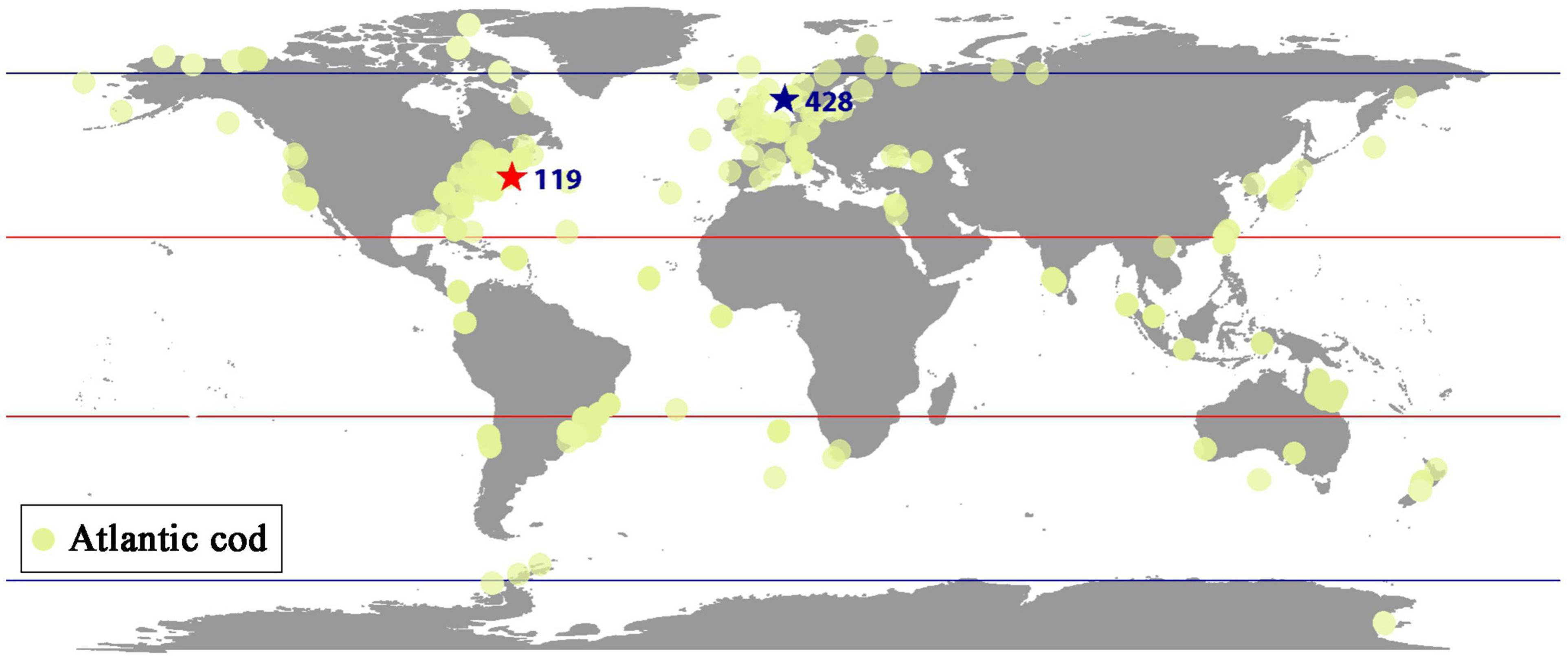
Figure 1. Global distribution of Atlantic cod.

TABLE 2

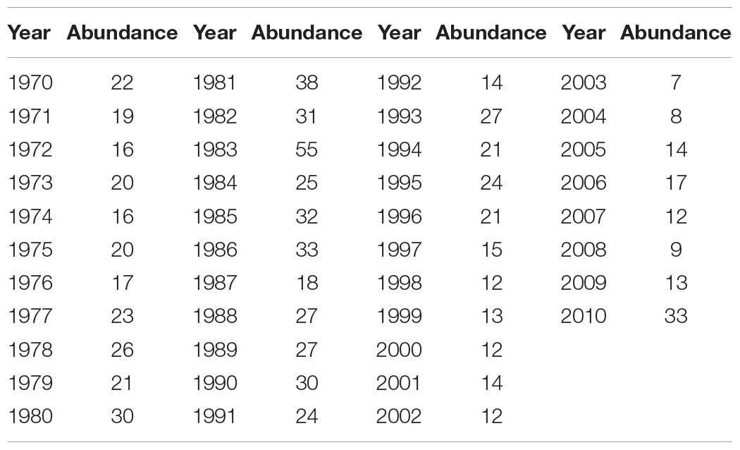
Table 2. Annual average abundance of Atlantic cod at site 119.

TABLE 3

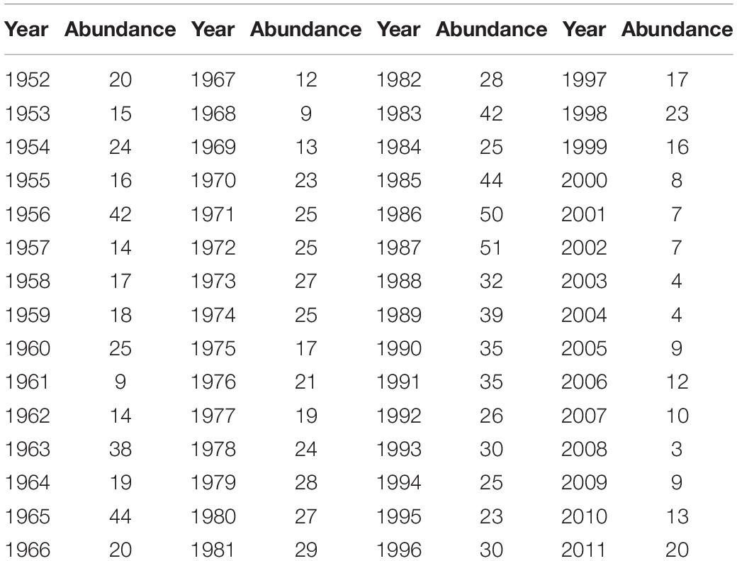
Table 3. Annual average abundance of Atlantic cod at site 428.

Sea Surface Temperature

Sea surface temperature can be considered as one of the most essential climate indicators of abundance variation in Atlantic cod. The global monthly SST available from the SST version 5 (ERSST.v5) dataset of the NOAA Climate Center is produced by a monthly extended reconstruction of SST observations from the Comprehensive Ocean-Atmosphere Data Set (COADS) and can be tracked back to the mid-19th century. Since SST adopts smooth local and short-term changes, with many options in quality control, deviation adjustment, and interpolation having been substantially revised, it is suitable for long-term global studies. In order to focus on the local annual SST at both site 119 and site 428, we made use of the geographic midpoint and selected the closer temperature points associated with it, with the spatial distance less than 2° in latitude and longitude. The Atlantic cod abundance at each site is only recorded in certain months of the year, i.e., February, March, July, and October at site 119, and September and October at site 428. Therefore, we finally retrieved the corresponding annual SST through the spatial averaging of the relevant nearby points and the time averaging of a specific month, for site 119 from 1970 to 2010 and site 428 from 1952 to 2011.

Sea Surface Salinity

The global monthly SSS is procurable by the quality-controlled ocean salinity profiles in the EN4 database from Met Office Hadley Centre, covering the time period from 1900 to present. We retrieved the annual SSS at both site 119 and site 428 in the same process as the annual SST, namely, by spatial averaging and time averaging after collating the relevant salinity points around the geographical midpoint of each site.

Atlantic Cod Catches

The global annual catches of Atlantic cod have been extracted via Food and Agriculture Organization Statistical Database (FAOSTAT). The Atlantic cod catch records at all observation sites since 1952 to 2011 have first been retrieved and then we selected the observation stations relevant to geographic midpoint of each site in study, with relatively complete records. Due to fishing prohibition in specific months, e.g., the spawning season of Atlantic cod, we could not collect the catches for every month, but the total number in each year. The annual average catches could be calculated by spatial averaging of neighboring observation stations.

Prey Biomass

For the prey biomass of Atlantic cod at each site, we first compiled the primary prey abundance via BioTIME database, such as herring, hairscales, capelin, and various zooplankton and invertebrates, and carried out the same screening process as Atlantic cod abundance, i.e., deleting duplicates, zero abundance counts, and abiotic records, as well as eliminating singular values through mathematical expectations. Finally, the annual prey biomass of each site has been derived by accumulating the abundance of all prey generated by time averaging.

Methods

Basic Wavelet Analysis

The basic wavelet analysis decomposes the abundance of Atlantic cod in the form of time series into a superposition of wavelet functions, all of which are derived from a mother wavelet function through translation and scaling. Let A(t) be the abundance of Atlantic cod time series, the irregularity of the wavelet function can approximately reflect the sharp non-stationary changes in Atlantic cod abundance A(t), and hereby more realistically describe the original dynamics at a certain time scale:

${\mathrm{\varphi }}_{a,\mathrm{\tau }}(t)=\frac{1}{\sqrt{a}}\mathrm{\varphi }\left(\frac{t-\mathrm{\tau }}{a}\right)(a,\mathrm{\tau }\in R,a>0)(1)$

$\text{with}\mathit{\hspace{1em}}{\int }_{-\mathrm{\infty }}^{+\mathrm{\infty }}\mathrm{\varphi }(t)\mathit{d}t=0(2)$

where ϕ(t) is a mother wavelet function, ϕ(t) ∈ L²(R), which refers to a type of oscillation function that can quickly decay to zero and could take many forms, such as Haar wavelet, Morlet wavelet (Goupillaud et al., 1984), Daubechies wavelet (Daubechies, 1991), Meyer wavelet (Meyers et al., 1993), Mexican straw hat wavelet (Torrence and Compo, 1998), and so on. ϕ_a,τ(t) is a sub-wavelet, a is a scale factor, representing the period length of the wavelet, and τ is a shift factor, reflecting the shift in time. In view of the abundance variation of Atlantic cod at multiple time scales, we try to focus on the principle of continuous wavelet transform over time:

$W_A(a,\mathrm{\tau })=\frac{1}{\sqrt{a}}{\int }_{R}A(t)\overline{\mathrm{\varphi }}\left(\frac{t-\mathrm{\tau }}{a}\right)\mathit{d}t(3)$

where W_A(a,τ) is the wavelet transform coefficient.

Periodicity

In order to discover the potential periodicity embedded in Atlantic cod abundance A(t), it is more desirable to achieve smooth wavelet amplitude by a non-orthogonal wavelet function, while the complex wavelet transform could provide both phase and amplitude to help with it (Torrence and Compo, 1998). We apply Morlet wavelet as our mother wavelet which not only has non-orthogonality but also has exponential complex wavelet adjusted by Gaussian. The Morlet wavelet function can be denoted as follows:

${\mathrm{\varphi }}_0(t)={\mathrm{\pi }}^{-1/4}{e}^{i{w}_{0}t}{e}^{-t^2/2}(4)$

where t represents the time variable and w₀ is a dimensionless frequency.

The modulus and modulus square of wavelet coefficients can first determine certain range of periodicity of global Atlantic cod abundance A(t) at multiple time scales. The modulus of the Morlet wavelet coefficient can be considered to be a reflection of the energy density distribution in the time domain. The greater the modulus, the stronger the periodicity of the global Atlantic cod abundance. We could hereby take it as one historic evidence to evaluate the future trend of global Atlantic cod abundance A(t) at multiple time scales. The wavelet spectrum of Atlantic cod abundance A(t) can be defined as:

${\left|W_A(a,\mathrm{\tau })\right|}^2=W_A(a,\mathrm{\tau })W_A^{*}(a,\mathrm{\tau })(5)$

where |W_A(a,τ)| and $W_A^{*}(a,\mathrm{\tau })$ are the modulus and the complex conjugate of the wavelet coefficient W_A(a,τ).

The variance of the wavelet coefficients could help determine the periodicity in a more exact way, so here we further integrate all squared values of the wavelet coefficients with scale a in the time domain as follows:

$Var(a)={\int }_{-\mathrm{\infty }}^{+\mathrm{\infty }}{\left|W_A(a,\mathrm{\tau })\right|}^2\mathit{d}\mathrm{\tau }(6)$

Wavelet Coherence

Let T(t) be the corresponding SST time series. The cross-wavelet transform between Atlantic cod abundance A(t) and SST T(t) can be represented as:

$W_{AT}(a,\mathrm{\tau })=W_A(a,\mathrm{\tau })W_T^{*}(a,\mathrm{\tau })(7)$

where W_A(a,τ) and W_T(a,τ) are, respectively, the wavelet transforms of A(t) and T(t), and $W_T^{*}(a,\mathrm{\tau })$ indicates the complex conjugation of W_T(a,τ). The covariance between the cross-wavelet power spectrum is then defined as follows:

$\left|W_{AT}(a,\mathrm{\tau })\right|=\sqrt{\left|W_A(a,\mathrm{\tau })\right|\left|W_T^{*}(a,\mathrm{\tau })\right|}(8)$

Assuming the potential periodicity of Atlantic cod abundance, we try to expand the total finite length of time series to deal with the edge effect; there will exist the discontinuities at the edges with the decrease of the amplitude in the wavelet power spectrum, which is specified as the Cone of Influence (COI). Since the results in COI will be affected by boundary distortion, reliable information cannot be provided and should be removed.

The correlation between Atlantic cod abundance and SST could be further measured via wavelet coherence (Torrence and Webster, 1999), as follows:

$C_{AT}(a,\mathrm{\tau })=\frac{\left|S(W_{AT}(a,\mathrm{\tau }))\right|}{\sqrt{S({\left|W_{AA}(a,\mathrm{\tau })\right|}^2)•S({\left|W_{TT}(a,\mathrm{\tau })\right|}^2)}}(9)$

where S(W_AT(a,τ)) is the cross spectral density between A(t) and T(t). The wavelet coherence coefficient reflects the synchronization similarity, i.e., co-movement between two time series, or whether the variation law takes on a linear relationship. The higher wavelet coherence is, the stronger the correlation is.

Meanwhile, the wavelet phase differences capture negative and positive correlation directions and depict the possible lead-lag effects among two time series:

${\mathrm{\psi }}_{AT}={\tan }^{-1}\left(\frac{I\left\{S(W_{AT}(a,\mathrm{\tau }))\right\}}{R\left\{S(W_{AT}(a,\mathrm{\tau }))\right\}}\right),{\mathrm{\psi }}_{AT}\in [-\mathrm{\pi },\mathrm{\pi }](10)$

where Iand R are the imaginary and real parts of the smoothed cross-wavelet transform, respectively. If ψ_AT is zero, the two series co-move together (in-phase), and if it is π (or −π), they co-move in opposite directions (out of phase). If ψ_AT ∈ (0,π/2), they positively co-move, and A_(t) leads T_(t); if ψ_AT ∈ (π/2,π), they negatively co-move, and T_(t) leads A_(t); if ψ_AT ∈ (−π,−π/2), they negatively co-move, and A_(t) leads T_(t); if ψA_T ∈ (−π/2,0), they positively co-move, and T_(t) leads A_(t). The abovementioned wavelet coherence can also be extended to evaluate the mutual relationship between Atlantic cod abundance and other extrinsic indices, including Atlantic cod catches C_(t), prey biomass B_(t), and SSS S_(t).

LSTM-SAE

We employ LSTM as an optimized recurrent neural network that allows to capture and retain long-term dependencies between Atlantic cod abundance A_(t) and other extrinsic indices, and meanwhile concludes the mutual relationship between the historic and current linkage effectively. Let the multivariate input vector be the combination of all or parts of time series from Atlantic cod abundance, SST, catches and prey biomass, and SSS in the time step _t, and the output vector be the label from Atlantic cod abundance itself in the next time step _{t + 1}. The advantage of the LSTM structure is that three types of gates, i.e., the input gate, output gate, and forget gate, are included, which could allow the storage of time series of Atlantic cod abundance and the external impact factors over a long-term period and also solve the vanishing gradient problem. Let _{X^t = [A^t,T^t,C^t,B^t,S^t]} and _{y^t = A^{t + 1}} be the input and output of LSTM unit at a certain time point _t, then the following calculation is performed,

$\begin{array}{c}{i}^t=\mathrm{\sigma }(G_i\times X^t+R_i\times y_L^{t-1}+b_i)\hfill \\ f^t=\mathrm{\sigma }(G_f\times X^t+R_f\times y_L^{t-1}+b_f)\hfill \\ o^t=\mathrm{\sigma }(G_o\times X^t+R_o\times y_L^{t-1}+b_o)\hfill \\ z^t=\mathrm{\sigma }(G_z\times X^t+R_z\times y_L^{t-1}+b_z)\hfill \\ c^t=i^t\odot z^t+c^{t-1}\odot f^t\hfill \\ y^t=o^t\odot \tan (c^t)\hfill \end{array}(11)$

where G_i, G_o, G_f, G_z, R_i, R_o, R_f,R_z, b_i, b_o, b_f, and b_z are, respectively, the weights of the input, the shared recurrent weights, and the bias weights for the three types of gates and input unit; i^t, f^t, o^t, and z^t are, respectively, the output of the three types of gates and input unit; c^t is the cell state of LSTM unit; σ represents the sigmoid activation function; and ⊙ is the Hadamard product, which refers to the element-wise product among matrices.

LSTM-based stacked autoencoder replaces random initialization strategies by applying stacked auto-encoder (SAE) into deep LSTMs in an unsupervised pre-training manner. As is shown in Figure 2, LSTM-SAE consists of three conventional shallow LSTM-AEs (LSTM-based autoencoder), which not only enhances the non-linear characteristics and compresses the input dimension, but also circumvents the expression limitations in multivariate prediction.

FIGURE 2

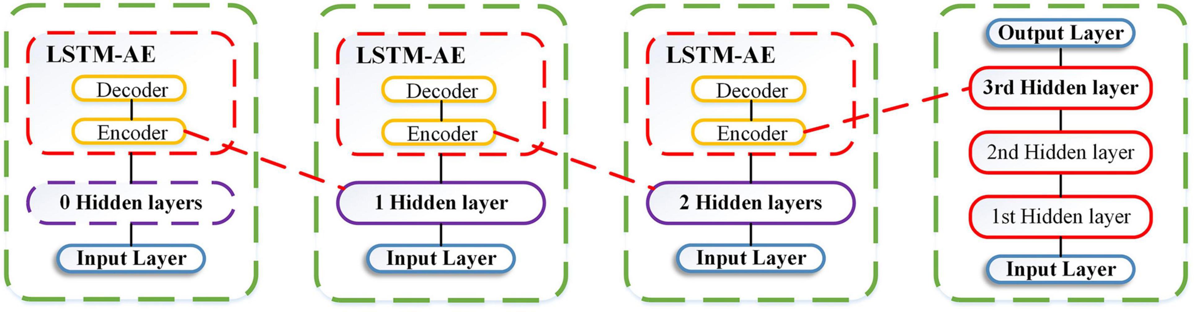
Figure 2. LSTM-SAE model.

The LSTM-AE module comes from the basic autoencoder (AE), which is originally sequentially connected as three layers in an unsupervised learning paradigm. The training procedure consists of two phases: encoding, in which the input is mapped into the hidden layer, and decoding, in which the input is reconstructed from the compressed representation. Given an unlabeled input X^t, it can be formulated as follows:

$h_1=f(w_1{X}^t+b_1)(12)$

$\stackrel{\mathrm{\wedge }\phantom{t}}{X^t}=w_2{h}_1+b_2(13)$

where h₁ represents the hidden encoder vector calculated from the input vector X^t, and $\stackrel{\mathrm{\wedge }\phantom{t}}{X^t}$ is the decoder vector of the output layer. Additionally, f is the activation function, w₁ and w₂ are the weight matrix of the encoder and decoder, and b₁ and b₂ are the bias vectors in each phase, respectively. The process of training is to minimize the reconstruction error; i.e., the cost function of each LSTM-AE module can be written as the difference between the original input X^t and the reconstructed time series $\stackrel{\mathrm{\wedge }\phantom{t}}{X^t}$.

LSTM-based stacked autoencoder sequentially combined and superposed shallow LSTM-AEs into deep learning networks through layer-by-layer greedy methods. The learning process consists of a pre-training phase and a fine-tuning phase. In the pre-training stage, we train the first LSTM-AE module in the stack and save its LSTM encoder layer as the input of the second LSTM-AE module, the second LSTM-AE module in the stack is trained with the encoded version of inputs loaded, and its LSTM encoder layer is saved as the input of the third LSTM-AE module. The purpose of reconstructing the original input instead of using the coded input of the previous layer is to strengthen the encoder to learn the characteristics of the original input. The original input is encoded twice by loading the encoder saved in the first two layers to train the third LSTM-AE module. We reconstruct the original inputs, not the encoded inputs, in order to enforce the encoder to learn the features of the inputs. Finally, we manage to initialize the three saved LSTM encoders and feed the real multivariate input in the time step t, together with the expected output of Atlantic cod abundance in the next time step t + 1, to learn in a supervised learning fashion during the fine-tuning stage.

Results

Periodicity

The periodicity estimation has been performed from 1919 to 2016 on the global annual average abundance of Atlantic cod derived by BioTIME via wavelet coefficients, on the basis of Morlet wavelet base. In order to offset the boundary effect of the specified region of COI, the extended time series at both ends has been employed for the wavelet transform coefficient. The symmetrical expansion around both ends for Atlantic cod abundance was first done within the time domain. After eliminating the expansion, the real part of the retained wavelet coefficient was made up of the wavelet coefficient contour map, as demonstrated in Figure 3, with the abscissa representing time and the ordinate referring to the time scale.

FIGURE 3

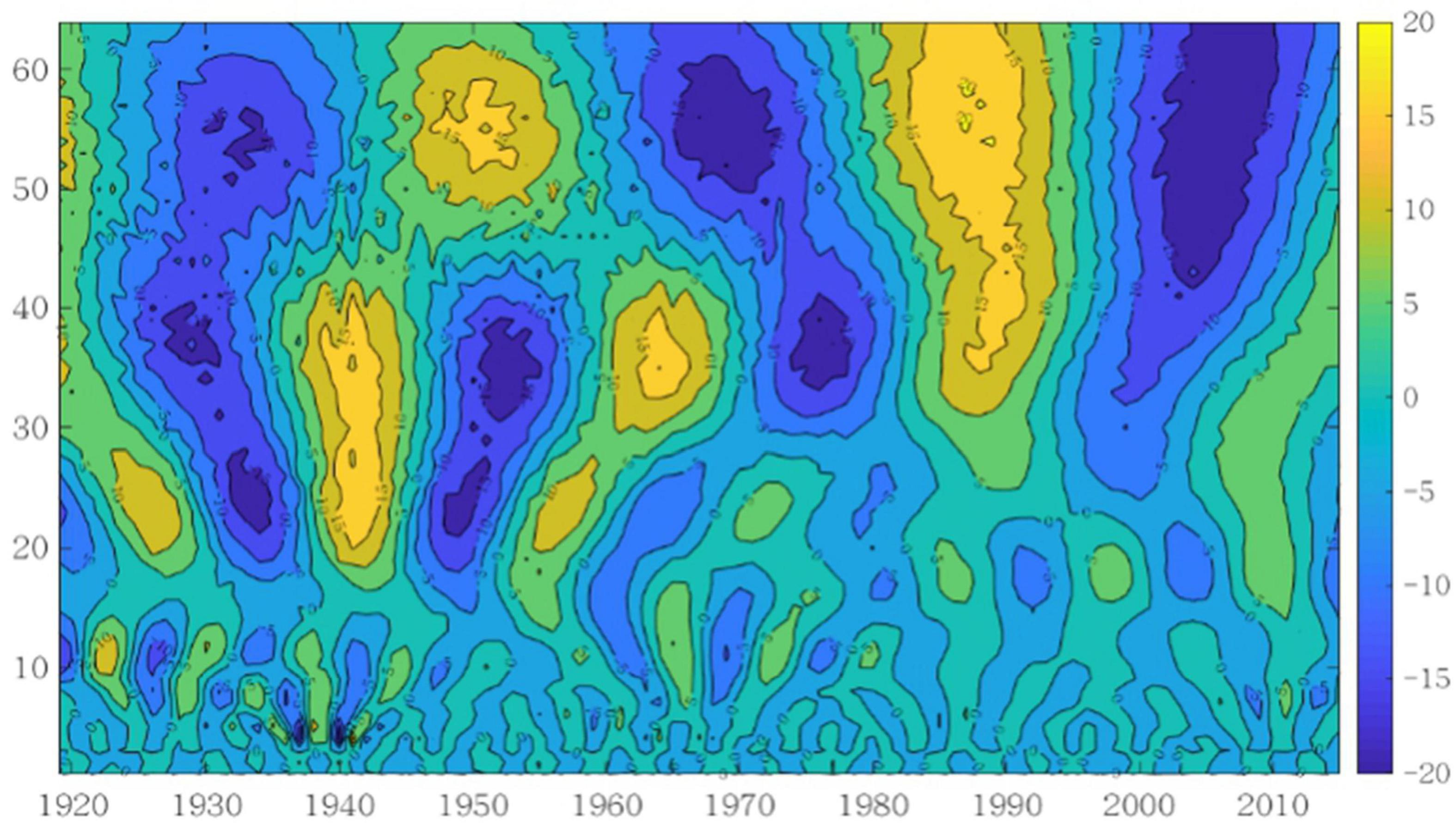
Figure 3. Contour map of wavelet coefficient.

It has been found from the wavelet coefficient contour map in Figure 3 that there exist three types of period variation of global Atlantic cod abundance at multiple time scales, i.e., 17–30 years, 30–45 years, and 45–64 years. Among them, at the time scale of 17–30 years, the global Atlantic cod abundance fluctuates abundantly, but the corresponding real value of wavelet coefficients is smaller, indicating that the periodicity is less obvious. At the time scale of 30–45 years, Atlantic cod abundance has experienced four fluctuations from rich to poor period according to the reflection of the oscillation intensity. Considering that there is a hidden period, the real value of wavelet coefficients is medium. At the time scale of 45–64 years, the global Atlantic cod abundance has the most obvious periodic variation in rich and poor periods, and the real value of wavelet coefficients is relatively large. Three poor centers of the oscillation intensity, 1930, 1970, and 2005, and two rich centers, 1950 and 1985, have been discovered. The periodic variation of the last two time scales behaved relatively stably throughout the time domain of the Atlantic cod abundance time series in study, while the first time scale was relatively weak and only stable before the 1960s.

We also applied the wavelet energy spectrum to analyze the evolution of oscillation energy at different periods in global Atlantic cod abundance. The modulus and modulus square maps of the wavelet coefficients are illustrated in Figure 4, where the largest values correspond to the 45- to 64-year time scale, especially since 1960, indicating that there is a major period and the periodicity of global Atlantic cod abundance is more stable. At the time scale of 30–45 years, there is a minor period from 1919 to 1990 accordingly, with relatively small values of the modulus and modulus square. Similarly, the periodicity emerges at the time scale of 17–30 years from 1919 to 1960.

FIGURE 4

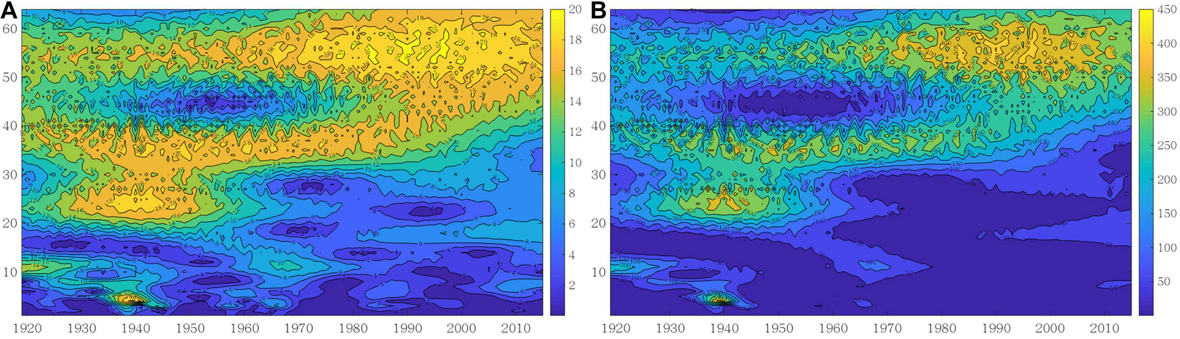
Figure 4. Wavelet contour map with Morlet wavelet. (A) Modulus of wavelet coefficient. (B) Modulus square of wavelet coefficient.

The wavelet variance map proportionally reflects the distribution of fluctuating energy in Atlantic cod abundance time series at multiple time scales and can be employed to derive the time periods in the evolution process, as shown in Figure 5A. There exist four obvious peaks in the wavelet variance map, which in turn correspond to the time scales of 55, 37, 24, and 11 years, i.e., the highest of the first major period in Atlantic cod abundance variation, as well as the second to third, fourth highest peak. The fluctuations of the above four periods influence the variation characteristics of Atlantic cod abundance in the entire time domain, where the first and the second periods play dominant roles, and the third and fourth periods only have minor effects for reference because of their small value in variance curves.

FIGURE 5

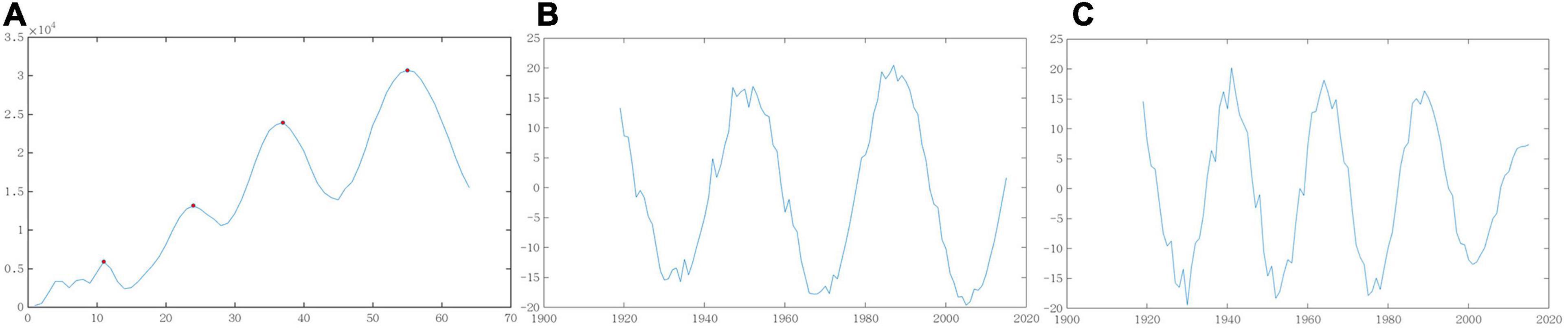
Figure 5. Variance and periodic map of wavelet coefficients. (A) Wavelet variance. (B) The first cycle. (C) The second cycle.

We further characterized and developed the trend graph of the first and second periods for global Atlantic cod abundance at two time scales. From the test results of the wavelet variance in Figures 5B,C, it has been illustrated that there appear the characteristics of global Atlantic cod abundance lasting about 36 years within an average period at the 55-year time scale, with roughly 2.7 periods in rich and poor, respectively. At the 37-year time scale, the average period of global Atlantic cod lasts around 24 years with four periods; the stability of this time period is relatively poor, but the overall periodicity is still very obvious. We could hereby make use of the inherent periodicity tendency of global Atlantic cod abundance to explore its potential alternating fluctuation patterns along time, providing a basis for the abundance prediction itself.

Wavelet Coherence

We utilized the wavelet coherence to search for how the co-movement between Atlantic cod abundance and the extrinsic indices performs over time and described the lead-lag effects through the wavelet phase difference. The wavelet coherence and phase difference map of Atlantic cod abundance with SST, catches, prey biomass, and SSS at sites 119 and 428 are, respectively, shown in Figures 6, 7, where wavelet correlation is affected by discontinuity, and the color bar corresponds to the relative intensity of each frequency (the stronger correlation tends to be in red, while the weaker correlation tends to be in blue), the edge COI is denoted in thick black curve, and 5% and 10% significance levels are, respectively, represented by a black thin line and a black dashed line.

FIGURE 6

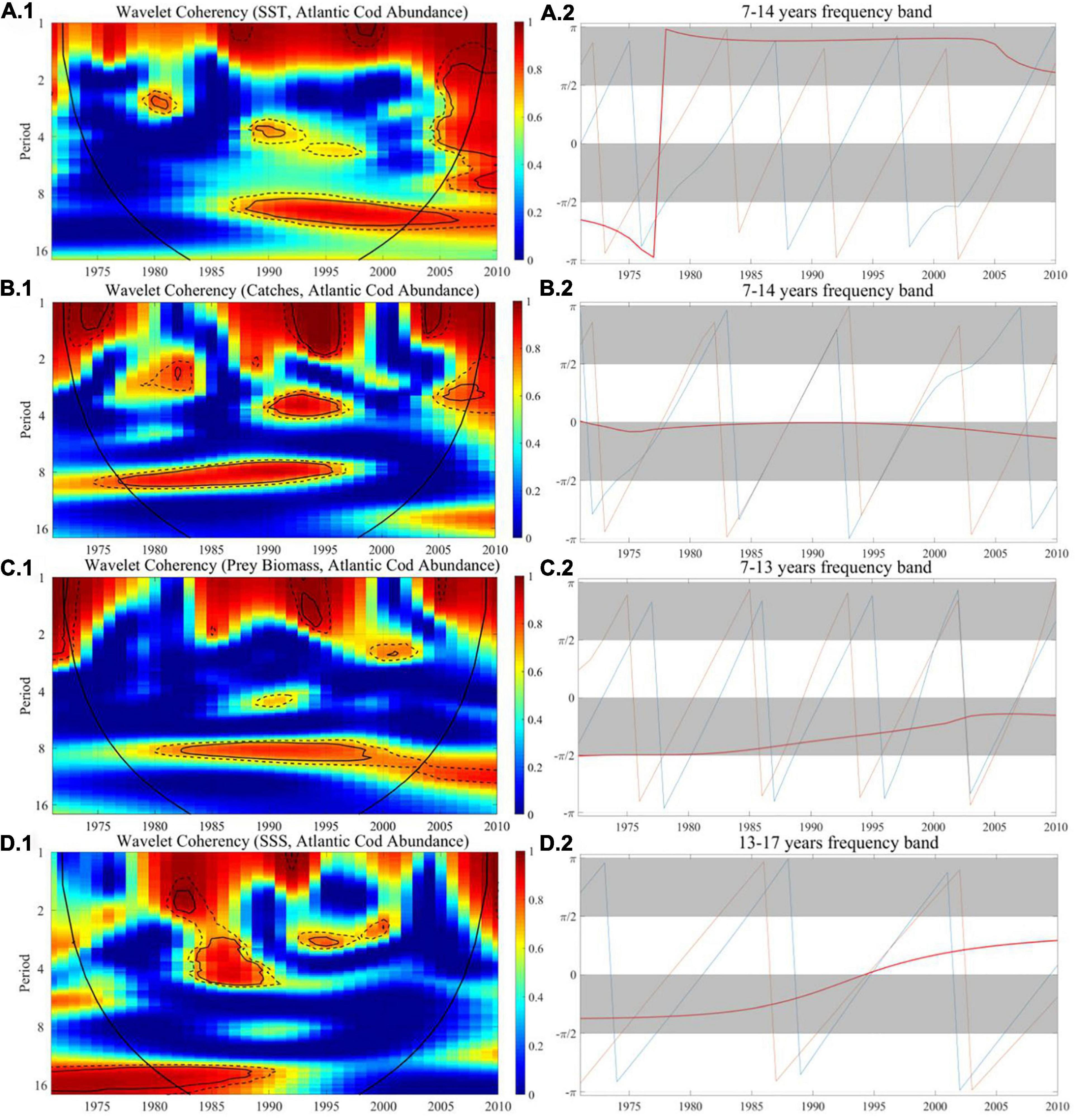
Figure 6. The wavelet coherence and phase difference between Atlantic cod abundance and SST, catches, prey biomass, and SSS at site 119. (A–D.1) Wavelet coherence and (A–D.2) phase difference. The y-axis refers to frequency (in years), and the x-axis refers to the time period.

FIGURE 7

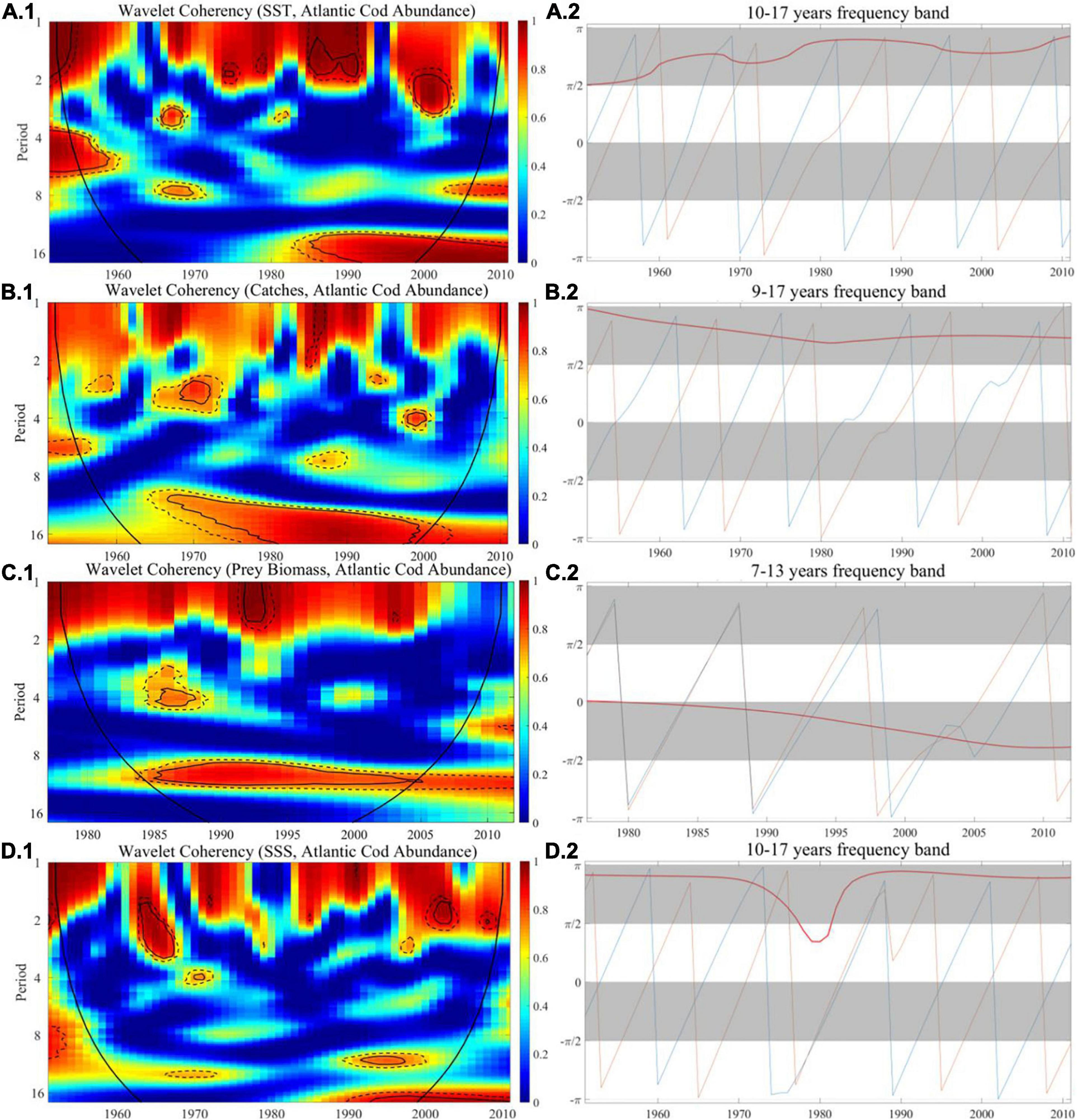
Figure 7. The wavelet coherence and phase difference between Atlantic cod abundance and SST, catches, prey biomass, and SSS at site 428. (A–D.1) Wavelet coherence and (A–D.2) phase difference. The y-axis refers to frequency (in years), and the x-axis refers to the time period.

For Atlantic cod abundance vs. SST, in Figure 6A.1, from the perspective of long-term frequency, the correlation coefficient at site 119 in the 7- to 13-year band is greater than 0.95 after 1987, indicating that there exists a significant long-term correlation and then the degree of correlation coefficients begins to decline after 2003. In Figure 7A.1, there is a significant correlation at site 428 in the 10- to 15-year band from 1985 to 2000, and the correlation coefficient reached more than 0.95. In the short-term frequency band, the correlation at both sites is not obvious. Meanwhile, in the long-term frequency band, the phase difference at both sites is in the range of π/2 to π throughout the period when the correlation is strong, which implies that there is a significant negative correlation between the two time series at both sites 119 and 428.

For Atlantic cod abundance vs. catches, in Figure 6B.1, with reference to the wavelet coherence map, we found that it exceeded 0.95 at site 119 in the 1- to 5-year band in the 1990s, indicating significant correlation in the short term. In the long-term frequency band of 7–14 years, this significant correlation lasted from 1977 to 1995, with the coefficient greater than 0.95, and there was no obvious correlation thereafter. In Figure 7B.1, the two time series is significantly correlated at site 428 in the 9- to 15-year frequency band almost throughout the sampling period, especially in the period from 1966 to 2000 when the significance ratio reached its peak, with the correlation coefficient exceeding 0.95. The coherence map displays a common significant correlation at both sites from the 1970s to the mid-1990s, while the correlation at site 428 lasted longer, until 2000. The phase difference described that, in the long-term frequency band, the two time series at site 428 are significantly negatively correlated throughout the time period, while the phase difference at site 119 in the frequency band of 7–14 years is close to zero during the entire period, indicating that the two time series are approximately moving in synchronization, and at both sites, Atlantic cod caches tend to dominantly lead its changes in abundance.

For Atlantic cod abundance vs. prey biomass, in Figure 6C.1, the correlation coefficient at site 119 in the long-term frequency band of 7–13 years was about 0.9 from 1982 to 1998, but in the short term, there is no obvious connection being displayed. In Figure 7C.1, the coherence map shows significant correlation at site 428 in the long-term frequency band from 7 to 13 years during almost the entire time period. The correlation coefficient is greater than 0.9 around the 1990s, and began to decline after 2005, indicating that the correlation was most significant from the mid-1980s to the end of the last century. The phase difference demonstrates that there is a significantly positive correlation between two time series at both sites during the entire co-movement period, and the Atlantic cod prey biomass tends to dominantly lead its changes in abundance.

For Atlantic cod abundance vs. SSS, in Figure 6D.1, from the coherence map, we could find that there is a significant correlation in the 3- to 5-year band at site 119 from 1983 to 1989, but after that, it turned to a weak correlation. In the long run, this correlation becomes more significant in the frequency band of 13–17 years, with the coefficient close to 1, and lasts from 1980 to 1988, but after that, this correlation was not obvious. In Figure 7D.1, the correlation coefficient at site 428 in the long-term frequency band of 10–17 years exceeded 0.9 from 1990 to 2000, while before 1990, the correlation coefficient was generally less than 0.6. In the short term, this correlation is not obvious. The phase difference shows that the two time series at site 119 are positively correlated throughout the period of co-movement, while at site 428, they are more probably negatively correlated. However, at both sites, SSS tends to dominantly lead its changes in abundance.

Discussion

First, it has been basically revealed from our experimental results that at both sites 119 and 428, SST began to have dominantly negative effects on the abundance variation of Atlantic cod since the 1980s. The increase of sea temperature actually exerted dramatic influences to the Atlantic cod abundance. For example, it has been investigated that from the 1980s to the beginning of the 21st century, the average SST and bottom temperature of the North Sea around site 428 have increased by 0.7°C and 0.15°C per decade (Walther et al., 2002; Sheppard, 2004). It has also been reported by NOAA that the North Atlantic Oscillation (NAO) index, i.e., the oscillation of atmospheric mass between the Arctic and the subtropical Atlantic, remains a positive phase since then, indicating the indirect consistency in its variation pattern on Atlantic cod (Brander and Mohn, 2004), e.g., the changes in the recruitment and spawning of Atlantic cod with the local environmental variables (Stige et al., 2006). At site 428, the annual SST from 1980 to 2000 was 10.5°C on average, an annual increase of 0.6°C from the 1970s, corresponding to the average decrease of Atlantic cod abundance by roughly 40%. In particular, due to the El Niño events in 1982–1983 and 1997–1998, the annual SST at site 428 both exceeded 12°C in the year 1983 and 1997, which exactly corresponds to the sharp drop in the abundance of Atlantic cod by 45% and 49%, respectively, compared to the entire 1970s. Similarly, the annual SST at site 119 in 1997 have reached 13.1°C, far exceeding the average values 10.3°C in the 1970s, and the corresponding abundance of Atlantic cod dropped by 56%. In total, 13 El Niño events have occurred globally from 1950 to 2000, 69% of them after 1980, demonstrating that the abundance variation of Atlantic cod is closely related to the changes of SST due to frequent activities of El Niño since the 1980s, which could be one of the significant reasons for the decline of Atlantic cod abundance after 1980.

Second, a strong positive correlation between the Atlantic cod abundance and its prey richness has been demonstrated from our experimental results at site 119 around 1980–2000 and at site 428 around 1985–2008. While the richness of marine primary producers decreased by 26% and 34% during the above time period, compared to the average values in the whole 1970s, the Atlantic cod abundance dropped by 40% and 47% correspondingly. We believe that there are two major reasons for the descent in the richness of primary producers. (1) The influence of the marine environment changes, such as the rising SST and the ocean acidification. Whether it is smaller zooplankton, invertebrates, or herring and capelin, most of them are more sensitive to changes in the marine environment. The abundance of small pelagic species, such as shrimp and capelin, decreases with increasing temperature, and even some zooplankton may have disappeared. For example, it has been investigated that the abundance of capelin in 1998 at Newfoundland around site 119 has particularly made a reduction of 55.3% compared to that in 1978 (Rose and O’Driscoll, 2002), and the corresponding abundance of Atlantic cod dropped by roughly 42% during the same period. (2) The increase in abundance of Atlantic cod competitors, such as those migrant predators in deep open waters, like moray, perch, tuna, etc. It has been reported that the abundance of these large fish species in the North Atlantic was not significantly affected by the increase in temperature, and even showed an increasing trend because of migration. For example, the SST of Celtic Sea to the south of Ireland had exceeded 12°C in 1992, causing some tuna to migrate northward to North Sea near site 428 (Hiddink and Ter Hofstede, 2008). The increase in the number and types of advanced species could be attributed to accelerate the rate of decrease of primary species richness. As the abundance variation of Atlantic cod basically produced responses to both the prey biomass and SST since the 1980s and continued to the present, the effect of prey biomass also indirectly proves the influence of SST, indicating that SST could not only cause a direct response, but may be an indirect response to the changes of Atlantic cod abundance.

Third, it is obviously shown from our experimental results that overfishing imposed tremendous influences on the abundance variation of Atlantic cod. The occurrence of highly correlative responses to Atlantic cod catches has been manifested from the 1960s to the end of the last century, at both sites 119 and 428; the strongest happened in the 1970s to the 1990s. For example, at site 119, the abundance of Atlantic cod has strongly followed the catches synchronously during 1975–1995, indicating that the catches played an actively guiding role in the abundance variation during this time period. In 1976, the catches of Atlantic cod at sites 119 and 428, respectively, increased by 32.2% and 19.1%, compared to that in 1960s, and the abundance of Atlantic cod decreased by 28.6% and 12.1% correspondingly. The dramatic increase in Atlantic cod catches since the early 1970s was mainly due to the rapid development of fishery technology. High-efficiency equipment such as ocean trawl and seine nets have been widely adopted (Valdemarsen, 2001). As a result, the world’s annual fish catches were more than quadrupled in the late 1970s. It has been investigated that the average annual catches of Atlantic cod in the Gulf of Maine near site 119 in the 1980s increased to 40,000 tons, more than four times that of the 1960s. However, there was a cliff-like decline of Atlantic cod catches after 1992, and the abundance of Atlantic cod increased by 18%, and then the average annual catches had returned to 10,000 tons after 2000 (Fogarty et al., 2008). There have been a series of ban policies issued from the 1990s in many countries, looking forward to seeing the abundance of Atlantic cod recover. Although, after years of limited fishing or even a ban on fishing, the scale of the local Atlantic cod showed no significant signs of rebound as expected in the end, it coincided with strong negative correlation at the beginning of its implementation.

Fourth, it has been demonstrated from our experimental results that SSS made great differences regarding the responses of the abundance variation in Atlantic cod at sites 119 and 428, respectively. On the one hand, at site 428, there mainly occurred a strong negative lead to Atlantic cod abundance after 1990. Since the increase in SSS is assumed to affect the activity of sodium and potassium ions in Atlantic cod, it might hereby cause the slow growth of Atlantic cod. In 2003, the SSS value at site 428 reached 36%, an increase of 7% compared to 1970, and at an average annual increase rate of 0.24% since then, while the abundance of Atlantic cod fell 47% during the corresponding time period. It has been reported that ocean evaporation (EVP) increased from the trough in 1977 to the peak in 2003 (Yu, 2007), which exactly coincides with the increase in SSS at site 428. In addition, the time–frequency co-movement of both SSS and SST at site 428 had the same tendency with the abundance variation of Atlantic cod after the 1990s. We believe that this is mainly because the rising SST causes the sea surface to evaporate more easily, so their correlation with Atlantic cod abundance was similar. On the other hand, at site 119, we have noticed that there was a strong positive correlation between SSS and Atlantic cod abundance mainly in the 1980s. For example, the SSS value at site 119 dropped from 32% in 1980 to 29% in 1983, and the abundance of Atlantic cod decreased by 27% during the corresponding time. We suppose that the decline in SSS in the corresponding period may be highly correlative to the influences of North American hurricanes in 1982. Humid climate, especially frequent rainfall during that time period, made it possible to lead to further SSS changes. It has been reported that Hurricane Alicia moved northward along the West Coast of the United States and Canada near site 119 in 1982 at an average wind speed of 95 mph, causing a 13-foot storm surge in the Gulf of Maine, with 6–12 inches of heavy rain.

The above external responses of the abundance variability run through the whole life history of Atlantic cod, and could be further attributed to the consistency with the simulation model or hypothesis that have been put forward. The warming and SSS reached deeper ocean due to strong mixing and convection associated to thermohaline circulation (Rahmstorf, 1995), which implied that the change in sea surface would also be transmitted to deeper habitat of Atlantic cod. The individual-based mechanistic model (Kristiansen et al., 2011) once incorporates the physical characteristics and the biological properties of the Atlantic cod larva and its surroundings, to assess the seasonal pattern of size variation of Atlantic cod eggs through adjusting environmental conditions of the mode. It has been shown from our experimental result that when SST at site 428 increased greatly in the 1990s, there was a significant negative correlation with Atlantic cod abundance. We could hereby presumably infer from the model that the size of Atlantic cod eggs might be reduced during that period and thus prolonged their hatching time and increased the possibility to be preyed. Combining with the Regional Ocean Modeling System (ROMS) (Shchepetkin and McWilliams, 2005), Vikebø et al. (2007) simulated the drift and distribution of Atlantic cod eggs and larvae. It has been shown from our experimental result that there was a dramatic decline in Atlantic cod abundance at site 428 during 2007–2008, and we could hereby infer that this might be related to the strong Norway current with large resolution motion in 2008 (Skagseth et al., 2008, 2011); the survival rate of Atlantic cod larvae was relatively reduced due to the long-term drift time. Árnason et al. (2013) have evaluated the growth rate of Atlantic cod under different salinity in a radioimmunoassay procedure and a protein assay kit, respectively. It has been shown from our experimental result that when SSS at site 428 increased obviously in 1997, there was a negative correlation with Atlantic cod abundance during this period. We could hereby assume that the continuous increase of SSS might have reduced the plasma cortisol level and the total plasma protein of Atlantic cod, resulting in the decrease of growth rate and even death of Atlantic cod. The probit regression model of Atlantic cod (Hutchings and Myers, 1994) classified maturing and spawning females and spent females, defined the time of spawning on which 50% of mature females were in a spent state, and described how the probability that a female will be spent was related to age at different seawater temperatures. It has been shown from our experimental result that at both site 119 and site 428, SST increased significantly around 1988–1992, and there was a negative correlation with the abundance. We could hereby estimate from the model that the higher seawater temperature might result in earlier Atlantic cod spawning through faster gonad development, which would indirectly lead to the drop in abundance. Wroblewski et al. (2000) monitored the activity of the tagged Atlantic cod in 1992 through an acoustic model and showed that the movement of Atlantic cod was related to the acoustically determined position of its prey and event structure in the local ocean currents. It has been shown from our experimental result that both the biomass of prey and the abundance of Atlantic cod exhibited a dramatically downward trend at site 119 in 1992. We could hereby suppose that in response to the Gulf Stream that moved northward through the Gulf of Maine, the prey shoal moved with the current (Johns et al., 1995), indirectly leading to the similar migration of Atlantic cod.

In general, in view of spatiotemporal interactions with SST, prey biomass, catches, and SSS around the recent 60 years, we conclude that the external responses of the abundance variability in Atlantic cod can be roughly divided into three distinguished stages: namely, the time period before 1985, 1985–1995, and after 1995. At the first stage, the reason for the decline in the abundance of Atlantic cod can be mainly attributed to the rapid rise of fish catches, due to the breakthrough of emerging advanced fishing technologies and its expansion in the fishery industry. In addition, in some observation sites, such as site 119, there were also strongly positive correlation effects from the relatively low SSS, while the impact of SST has not been highlighted, and even hardly observed. At the second stage, the abundance and catches of Atlantic cod still showed strong simultaneous moves, indicating that overfishing remained as one of the main factors. At the same time, warming SST began to be a significant index for the abundance variability in Atlantic cod, imposing both direct and indirect forces to the abundance, together with the significant impact of prey biomass changes and SSS. At the third stage, due to the beginning of fishing restrictions, protective measures, and policies, the impact of overfishing became relatively insignificant. The warming SST at sites 119 and 428 and the growing SSS in some areas such as site 428 directly lead to the decrease of Atlantic cod abundance, implying the increased sensitivity to changes in such marine environment factors.

The long-term dependency in the time series analysis above could quantitatively and systematically reveal the fundamental roles that those external elements responses to the abundance variability in Atlantic cod, and allow the identification of dominantly correlative factors for each stage. Concerning the self-correlated feedback that is always inherently underlined in the abundance itself, together with its periodicity, time–frequency co-movement, and lead-lag effects, we further capture the potentially predictive patterns and mechanism for abundance variation in Atlantic cod at each stage by constructing LSTM architecture. One group of LSTM-SAE units of diverse model selection have been employed to establish the predictive ensemble across stages, as shown in Figure 8. For each stage, we, respectively, pick only one input variable, i.e., Atlantic cod abundance itself, all the five input variables of correlative time series in our study, i.e., the Atlantic cod abundance, SST, SSS, prey biomass, and catches, as well as the particularly dominant indices at each stage, for training.

FIGURE 8

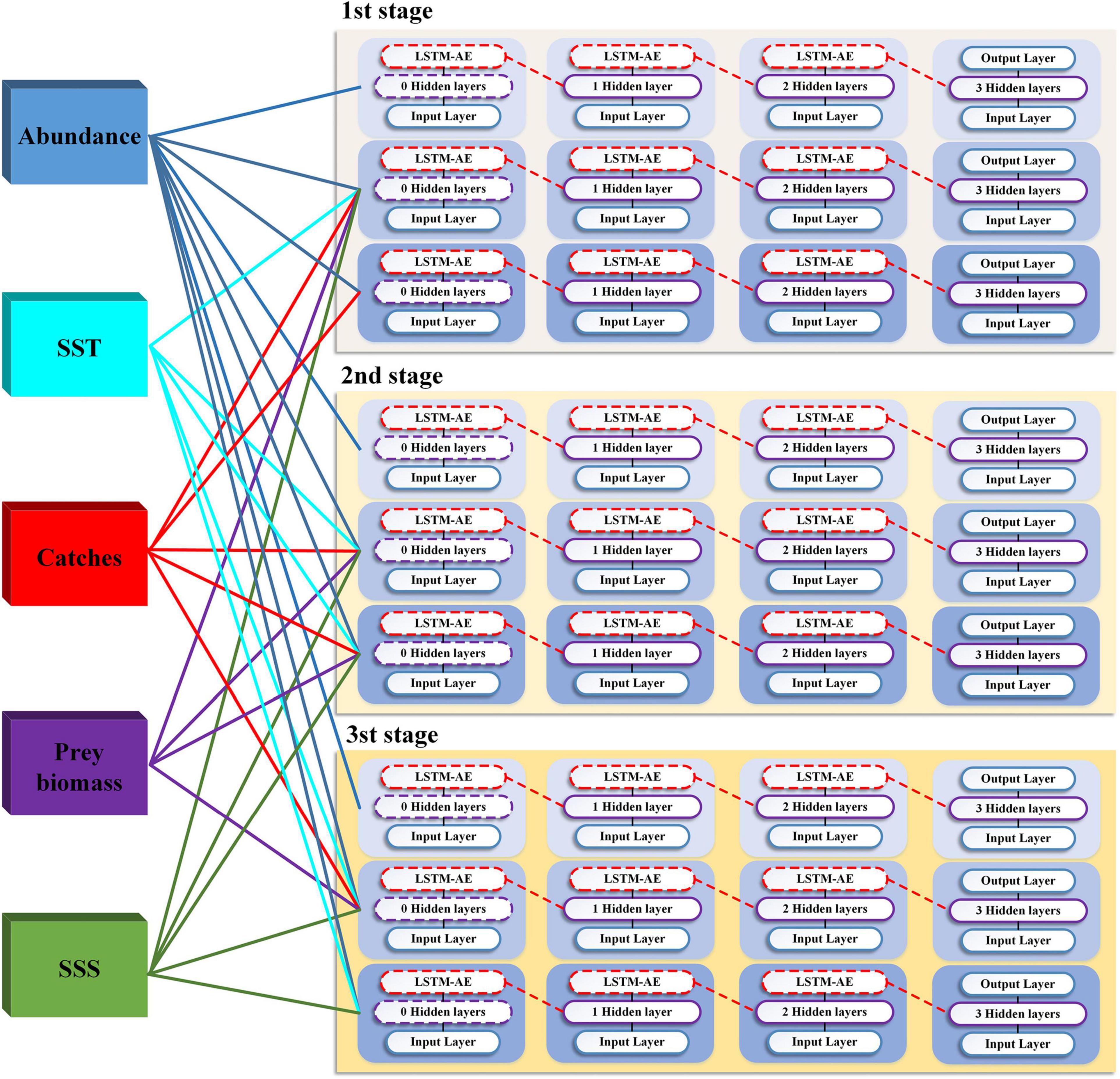
Figure 8. LSTM-SAE predictive ensemble.

Due to the scarcity of the records in all time series, one type of data augmentation is used, i.e., the Time-Conditional Generative Adversarial Network (T-CGAN), in which both the generator and the discriminator are conditioned on the sampling timestamps, to learn the hidden relationship between data and timestamps and consequently to generate new time series (Ramponi et al., 2018). At the same time, in order to eliminate the differences among dimensions, the common Min-Max normalization has also been taken to project the five input variables and speed up the convergence in the LSTM-SAE unit. In addition, the length of all the five types of time series, no matter the original and the augmented ones, remains identical, corresponding to the period 1952–2011. The total number of records is 2950 after the standardization and amplification process, including all of the five input variables, and then we divided the original time series dataset into three types, 60% for training, 15% for verification, and 25% for testing, to facilitate learning in the LSTM-SAE unit for a higher prediction accuracy.

Taking the prediction of Atlantic cod abundance at the observation site 428 as an example, we, respectively, select the dominantly correlative factors at three stages, i.e., Atlantic cod catches itself, all the four external impact factors, SST, and SSS, as the auxiliary input variables to help with the estimation, in a time domain of totally 59 observation years, with 43 years for training and verification, and 16 years for test. For each stage, we select three types of input vectors for training and testing, namely, Atlantic cod abundance, the additive dominantly correlative factors, and all the external impact factors. We applied both the classic LSTM and LSTM-SAE strategies in the ensemble into the time series of Atlantic cod abundance at site 428, and the corresponding prediction results at the third stage of 10-year duration from 1995 to 2011 are listed in Figure 9, where the ground truth is represented in blue solid line, and the solid and dashed lines in other colors stand for the prediction results of two models with respect to three types of input variables concerned, respectively. The prediction performances of the two competitive models have also been evaluated by means of RMSE, MAE, and symmetric mean absolute percentage error (SMAPE) measure, as listed in Table 4.

FIGURE 9

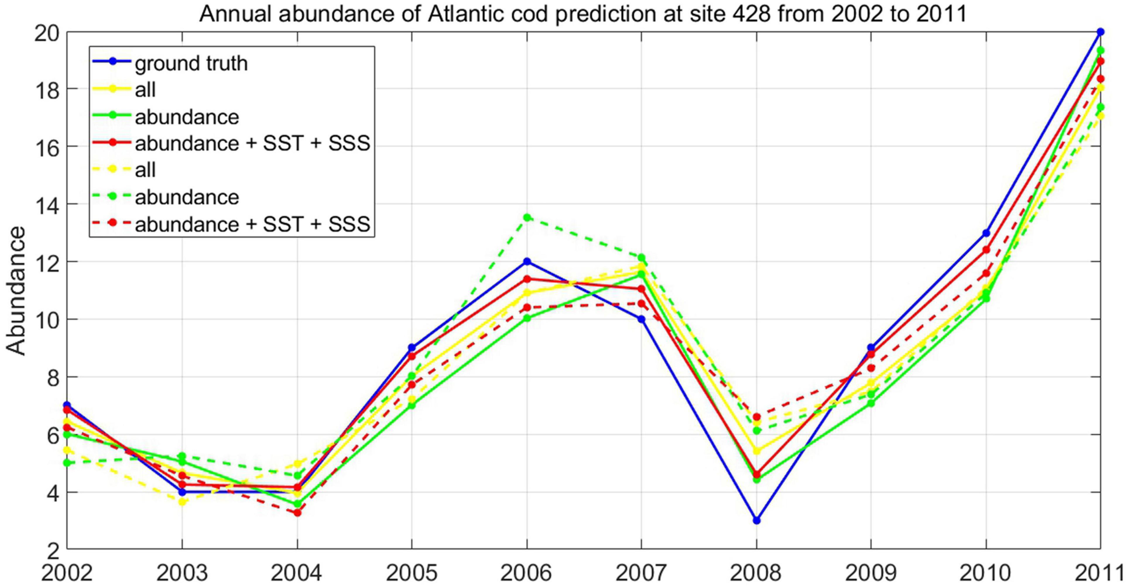
Figure 9. Prediction of Atlantic cod abundance.

TABLE 4

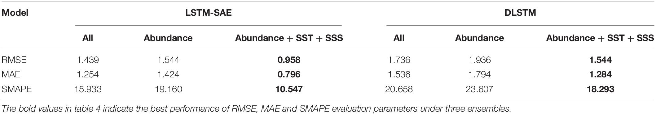
Table 4. Prediction performance comparison.

As it is mentioned above, we have made an initial attempt to explore the abundance prediction in Atlantic cod at site 428 for 1995–2011, and it could be seen from the experimental results that both LSTM-SAE and DLSTM models behaved better when applying multivariate prediction instead of only taking Atlantic cod abundance as the univariate input, with RMSE, MAE, and SMAPE of 0.958, 0.796, and 10.547 in LSTM-SAE and 1.544, 1.284, and 18.293 in the DLSTM model, respectively. It has also proved that the prediction process might perform slightly better when we intentionally select and feed with the dominantly correlative time series as the additional inputs, rather than all the referred external indices, indicating that there might exist relatively higher priority among all the other concerning variables at site 428 in the last decade; i.e., SST and SSS play relatively leading roles in determining the trend in Atlantic cod abundance to be predicted. Meanwhile, LSTM-SAE obviously exhibit better prediction performances compared to the classic DLSTM model for whatever type of training inputs, indicating that the impact of stacking LSTM in an auto-encoder fashion as one kind of pre-trained DLSTM has more advantages in Atlantic cod abundance prediction than the original DLSTM, which depends on most randomized initialization for LSTM.

The recent advances of deep neural network-powered, machine intelligence techniques provide a hopeful solution with the promise of end-to-end prediction modeling for the Atlantic cod abundance variation. First, we quantitatively and systematically reveal the fundamental roles of these external element responses to the abundance variability in Atlantic cod by analyzing the long-term dependencies in time series and allow them to identify dominantly correlative factors for each stage. Then, concerning the self-correlated feedback that is always inherently underlined in the abundance itself, together with its periodicity, time–frequency co-movement, and lead-lag effects, we further capture the potentially predictive hypothesis and mechanism for abundance variation in Atlantic cod at each stage. In the future, we could transfer such a comprehensive prediction mechanism to other sea areas, with the increase of the other influencing factors, and make an effective assessment of Atlantic cod abundance, which could hopefully provide a reference baseline for future fishery management and reasonable fishing decision-making.

Conclusion

As one of the economic fish species, Atlantic cod contributes significantly to the world’s total fishery production. Atlantic cod distributes in a wide range of habitats, and its survival mode has been influenced by multivariate factors, while most of the existing literature often concentrates on the discussion about the major univariate effects in the abundance variation of Atlantic cod. In this paper, we have quantitatively identified the spatiotemporal responses of Atlantic cod abundance across manifold intrinsic and extrinsic indices, on the basis of its periodicity, co-movement, and lead-lag effects, and then proposed to explore the potentially predictive mechanism about how Atlantic cod abundance would probably evolve over time in favor of LSTM. We have systemically retrieved the annual global abundance variation of Atlantic cod from 1919 to 2016 via BioTIME, and then selected the local observation sites, ID 119 and 428, with relatively complete abundance records for our study, and accordingly accessed and attained the other four external impact factors, i.e., the catches, the prey biomass, SST, and SSS, respectively, at specific geographical coordinates, by spatial and time averaging. We have provided evidences by integrating the modulus and variance of wavelet coefficients that the abundance variation of Atlantic cod will be influenced by its potential 36-year major cycle and 24-year secondary cycle at the time scales of 55 years and 37 years, respectively. We have generated the wavelet coherence map by the ratio between the wavelet cross-spectrum and power spectrum, and the phase difference by the ratio between the imaginary and the real part of the wavelet cross-spectrum, to evaluate the time–frequency co-movement and lead-lag effects over the external impact elements, and allow the identification of the dominantly correlative factors and capture the leading roles at each stage in the time domain. In view of spatiotemporal interactions, we further divided the responses of the abundance variation in Atlantic cod in the recent 60 years into three stages, namely, before 1985, 1985–1995, and after 1995. At the first stage, the reason for the decline in abundance can be mainly attributed to the rapid rise of fish catches. At the second stage, overfishing remained as one of the main factors, and the impact of SST and SSS also provides significant indices for the abundance variability; meanwhile, the mortality of primary producers and forced migration of fish species indirectly led to the decline. At the third stage, the impact of overfishing became relatively insignificant, and warming SST and growing SSS directly led to the decrease of abundance. It should be noted that we primarily consider the above critical external impact factors on the abundance variation of Atlantic cod from a long-term perspective, but we do not rule out the influences of the other factors, such as ocean acidification and marine microorganisms, which have not been involved in our study but could be taken into account in the future. Finally, with the help of historical spatiotemporal responses to manifold intrinsic and extrinsic indices, we have established the ensemble of LSTM-SAE architecture to comprehensively capture the predictive patterns possibly underlined in the variation of Atlantic cod abundance at each stage, by three types of input vectors, namely, Atlantic cod abundance, the additive dominantly correlative factors, and all the external impact factors. It has been demonstrated from the experimental results that the models behaved better when we intentionally select and feed with the dominantly correlative multivariate input, instead of all factors or only taking Atlantic cod abundance as the univariate input, with RMSE, MAE, and SMPE of 0.958, 0.796, and 10.547, respectively, when taking the prediction of Atlantic cod abundance during 1995–2011 at site 428 as an example. Meanwhile, LSTM-SAE obviously exhibits better prediction performances compared to the classic LSTM for whatever type of training inputs, indicating that the impact of stacking LSTM in an auto-encoder fashion has more advantages in Atlantic cod abundance prediction than the original LSTM. The proposed prediction strategies could not only symmetrically investigate the predictive attributes of the Atlantic cod abundance, potentially providing the quantitative references in reasonably making fishing decision, but also integrate evidences on its spatiotemporal responses of abundance variability and help explore the changes of biomass statistics, distribution, and biodiversity. Although the developed prediction scheme in our study still tends to be an initial attempt to understand the potential variation tendency of Atlantic cod abundance, we believe that it is quite reasonable to approximate the changes based on the past observations, in accordance with the direct and indirect external responses. Due to the rapid development of deep learning capabilities, it is to be hoped that understanding the abundance variability toward marine environment and anthropic forces could be further improved in the near future, and the public, the politicians, and the fishing industry could expect better and more quantitative predictions of the responses to global changes of not only Atlantic cod but other fish species and the ecosystem as a whole.

Data Availability Statement

Publicly available datasets were analyzed in this study. This data can be found here: BioTIME database for this study is available from the website (http://biotime.st-andrews.ac.uk) or through the Zenodo repository (https://zenodo.org/record/1095627); FAOSTAT database is retrieved in the website (http://www.fao.org/fishery/statistics/global-capture-production/query/en); ERSST.v5 database is available from NOAA website (https://www1.ncdc.noaa.gov/pub/data/cmb/ersst/v5), EN4 database can be available in the Met Office Hadley Centre observations website (https://www.metoffice.gov.uk/hadobs/en4/).

Ethics Statement

Ethical review and approval was not required for the animal study because all the data used in the study are publicly available.

Author Contributions

RN conceived and designed the study, contributed to analysis and interpretation of data, drafted the manuscript, and made final consent about the manuscript to be published. QY performed the main experimental work, contributed to analysis and interpretation of data, and drafted the manuscript. HH assisted in the experimental work and acquisition of data. XG helped with data statistics. CS provided guidance on experimental methods and data analysis. BH discussed and helped with the experiments. AL suggested the idea of the prediction mechanism. All authors contributed to the article and approved the submitted version.

Funding

This work was supported by the National Key R&D Program (2019YFC1408304), the National Program of International S&T Cooperation (2015DFG32180), the National High-Tech R&D 863 Program (2014AA093410), the National Natural Science Foundation of China (31202036), the National Science & Technology Pillar Program (2012BAD28B05), the National Key R&D Program (2016YFC0301400), and the National Natural Science Foundation of China (41376140).

Conflict of Interest

The authors declare that the research was conducted in the absence of any commercial or financial relationships that could be construed as a potential conflict of interest.

Acknowledgments

We would like to acknowledge team members Yu Cai and Jie Wang for their guidance in data analysis. We would also like to acknowledge Anne Magurran, Laura Antão, and Maria Dornelas for their support in availability of BioTIME.

References

Aguiar-Conraria, L., and Soares, M. J. (2011). Oil and the macroeconomy: using wavelets to analyze old issues. Empir. Econ. 40, 645–655. doi: 10.1007/s00181-010-0371-x

CrossRef Full Text | Google Scholar

Ames, E. P. (2004). Atlantic cod stock structure in the Gulf of Maine. Fisheries 29, 10–28.

Google Scholar

Árnason, T., Magnadóttir, B., Björnsson, B., Steinarsson, A., and Björnsson, B. T. (2013). Effects of salinity and temperature on growth, plasma ions, cortisol and immune parameters of juvenile Atlantic cod (Gadus morhua). Aquaculture 380, 70–79. doi: 10.1016/j.aquaculture.2012.11.036

CrossRef Full Text | Google Scholar

Baird, J. W., Bishop, C. A., and Murphy, E. F. (1991). Sudden changes in the perceptions of stock size and reference catch levels for cod in northeastern Newfoundland Shelves. Sci. Counc. Stud. 16, 111–119.

Google Scholar

Beaugrand, G., Lenoir, S., Ibanez, F., and Manté, C. (2011). A new model to assess the probability of occurrence of a species, based on presence-only data. Mar. Ecol. Prog. Ser. 424, 175–190. doi: 10.3354/meps08939

CrossRef Full Text | Google Scholar

Behrenfeld, M. J., O’Malley, R. T., Siegel, D. A., McClain, C. R., Sarmiento, J. L., Feldman, G. C., et al. (2006). Climate-driven trends in contemporary ocean productivity. Nature 444, 752–755.

Google Scholar

Berberidis, C., Aref, W. G., Atallah, M., Vlahavas, I., and Elmagarmid, A. K. (2002). “Multiple and partial periodicity mining in time series databases,” in Proceedings of the 15th Eureopean Conference on Artificial Intelligence, ECAI’2002, Vol. 2, Lyon, 370–374.

Google Scholar

Bogstad, B., Lilly, G. R., Mehl, S., Palsson, O. K., and Stefánsson, G. (1994). Cannibalism and year-class strength in Atlantic cod (Gadus morhua L.) in arcto-boreal ecosystems (Barents Sea, Iceland, and eastern Newfoundland). ICES Mar. Sci. Symp. 198, 576–599.

Google Scholar

Box, G. E., and Pierce, D. A. (1970). Distribution of residual autocorrelations in autoregressive-integrated moving average time series models. J. Am. Stat. Assoc. 65, 1509–1526. doi: 10.1080/01621459.1970.10481180

CrossRef Full Text | Google Scholar

Brander, K., and Mohn, R. (2004). Effect of the North Atlantic Oscillation on recruitment of Atlantic cod (Gadus morhua). Can. J. Fish. Aquat. Sci. 61, 1558–1564.

Google Scholar

Carey, C. C., Hanson, P. C., Lathrop, R. C., and St. Amand, A. L. (2016). Using wavelet analyses to examine variability in phytoplankton seasonal succession and annual periodicity. J. Plankton Res. 38, 27–40. doi: 10.1093/plankt/fbv116

PubMed Abstract | CrossRef Full Text | Google Scholar

Cloern, J. E., and Jassby, A. D. (2010). Patterns and scales of phytoplankton variability in estuarine–coastal ecosystems. Estuaries Coasts 33, 230–241. doi: 10.1007/s12237-009-9195-3

CrossRef Full Text | Google Scholar

Conover, R. J., Wilson, S., Harding, G. C. H., and Vass, W. P. (1995). Climate, copepods and cod: some thoughts on the long-range prospects for a sustainable northern cod fishery. Clim. Res. 5, 69–82.

Google Scholar

Dahlke, F. T., Leo, E., Mark, F. C., Pörtner, H.-O., Bickmeyer, U., Frickenhaus, S., et al. (2017). Effects of ocean acidification increase embryonic sensitivity to thermal extremes in Atlantic cod, Gadus morhua. Glob. Change Biol. 23, 1499–1510. doi: 10.1111/gcb.13527

PubMed Abstract | CrossRef Full Text | Google Scholar

Dajcman, S. (2013). Interdependence between some major European stock markets-a wavelet lead/lag analysis. Prague Econ. Pap. 22, 28–49. doi: 10.18267/j.pep.439

CrossRef Full Text | Google Scholar

Daubechies, I. (1991). “Ten lectures on wavelets,” in Proceedings of the CBMS-NSF Regional Conference Series in Applied Mathematics, (Philadelphia, PA: SIAM). doi: 10.1137/1.9781611970104

CrossRef Full Text | Google Scholar

Dey, R., and Salem, F. M. (2017). “Gate-variants of gated recurrent unit (GRU) neural networks,” in Proceedings of the 2017 IEEE 60th International Midwest Symposium on Circuits and Systems (MWSCAS), (Piscataway, NJ: IEEE), 1597–1600.

Google Scholar

Drinkwater, K. F. (2005). The response of Atlantic cod (Gadus morhua) to future climate change. ICES J. Mar. Sci. 62, 1327–1337. doi: 10.1139/f94-155

CrossRef Full Text | Google Scholar

Drinkwater, K. F., Frank, K., and Petrie, B. (2000). “The effects of Calanus on the recruitment, survival, and condition of cod and haddock on the Scotian Shelf,” in Proceedings of the ICES CM, 1000, 07 (Brugge: 2000 ICES Annual Science Conference).

Google Scholar

Duan, Y., Yisheng, L. V., and Wang, F. Y. (2016). “Travel time prediction with LSTM neural network,” in Proceedings of the 2016 IEEE 19th International Conference on Intelligent Transportation Systems (ITSC), (Piscataway, NJ: IEEE), 1053–1058. doi: 10.1109/ITSC.2016.7795686

CrossRef Full Text | Google Scholar

Fan, J., Li, Q., Hou, J., Feng, X., Karimian, H., and Lin, S. (2017). A spatiotemporal prediction framework for air pollution based on deep RNN. ISPRS Ann. Photogramm. Remote Sens. Spat. Inf. Sci. 4, 15–22. doi: 10.5194/isprs-annals-IV-4-W2-15-2017

CrossRef Full Text | Google Scholar

Fogarty, M., Incze, L., Hayhoe, K., Mountain, D., and Manning, J. (2008). Potential climate change impacts on Atlantic cod (Gadus morhua) off the northeastern USA. Mitig. Adapt. Strateg. Glob. Change 13, 453–466. doi: 10.1007/s11027-007-9131-4

CrossRef Full Text | Google Scholar

Freedman, D. A. (1981). Bootstrapping regression models. Ann. Stat. 9, 1218–1228.

Google Scholar

Fullard, K. J., Early, G., Heide-Jørgensen, M. P., Bloch, D., Rosing-Asvid, A., and Amos, W. (2000). Population structure of long-finned pilot whales in the North Atlantic: a correlation with sea surface temperature? Mol. Ecol. 9, 949–958. doi: 10.1046/j.1365-294x.2000.00957.x

PubMed Abstract | CrossRef Full Text | Google Scholar

Goupillaud, P., Grossmann, A., and Morlet, J. (1984). Cycle-octave and related transforms in seismic signal analysis. Geoexploration 23, 85–102. doi: 10.1016/0016-7142(84)90025-5

CrossRef Full Text | Google Scholar

Habernal, I., and Gurevych, I. (2016). “Which argument is more convincing? Analyzing and predicting convincingness of web arguments using bidirectional lstm,” in Proceedings of the 54th Annual Meeting of the Association for Computational Linguistics, Vol. 1: Long Papers, (Berlin: Association for Computational Linguistics), 1589–1599. doi: 10.18653/v1/P16-1150

CrossRef Full Text | Google Scholar

Haseeb, M., Abidin, I. S. Z., Hye, Q. M. A., and Hartani, N. H. (2019). The impact of renewable energy on economic well-being of Malaysia: fresh evidence from auto regressive distributed lag bound testing approach. Int. J. Energy Econ. Policy 9:269. doi: 10.32479/ijeep.7229

CrossRef Full Text | Google Scholar

Hays, G. C. (2017). Ocean currents and marine life. Curr. Biol. 27, R470–R473. doi: 10.1016/j.cub.2017.01.044

PubMed Abstract | CrossRef Full Text | Google Scholar

Hiddink, J. G., and Ter Hofstede, R. (2008). Climate induced increases in species richness of marine fishes. Glob. Change Biology 14, 453–460. doi: 10.1111/j.1365-2486.2007.01518.x

CrossRef Full Text | Google Scholar

Hinton, G. E., and Salakhutdinov, R. R. (2006). Reducing the dimensionality of data with neural networks. Science 313, 504–507. doi: 10.1126/science.1127647

PubMed Abstract | CrossRef Full Text | Google Scholar

Huang, G., Liu, Z., van der Maaten, L., and Weinberger, K. Q. (2017). “Densely connected convolutional networks,” in Proceedings of the IEEE Conference on Computer Vision and Pattern Recognition, Honolulu, HI, 4700–4708.

Google Scholar

Hutchings, J. A. (1996). Spatial and temporal variation in the density of northern cod and a review of hypotheses for the stock’s collapse. Can. J. Fish. Aquat. Sci. 53, 943–962. doi: 10.1139/f96-097

CrossRef Full Text | Google Scholar

Hutchings, J. A., and Myers, R. A. (1994). What can be learned from the collapse of a renewable resource? Atlantic cod, Gadus morhua, of Newfoundland and Labrador. Can. J. Fish. Aquat. Sci. 51, 2126–2146. doi: 10.1139/f94-214

CrossRef Full Text | Google Scholar

Jagannatha, A. N., and Yu, H. (2016). “Structured prediction models for RNN based sequence labeling in clinical text,” in Proceedings of the Conference on Empirical Methods in Natural Language Processing Conference on Empirical Methods in Natural Language Processing, Vol. 2016, (NIH Public Access), 856.

Google Scholar

Johns, W. E., Shay, T. J., Bane, J. M., and Watts, D. R. (1995). Gulf Stream structure, transport, and recirculation near 68 W. J. Geophys. Res. Oceans 100, 817–838. doi: 10.1029/94JC02497

CrossRef Full Text | Google Scholar

Jordaan, A. (2002). The Effect of Temperature on the Development, Growth and Survival of Atlantic cod (Gadus morhua) During Early Life-Histories, The University of Maine.

Google Scholar

Joy, M. K., and Death, R. G. (2004). Predictive modelling and spatial mapping of freshwater fish and decapod assemblages using GIS and neural networks. Freshw. Biol. 49, 1036–1052. doi: 10.1111/j.1365-2427.2004.01248.x

CrossRef Full Text | Google Scholar

Kirby, R. R., and Beaugrand, G. (2009). Trophic amplification of climate warming. Proc. R. Soc. B Biol. Sci. 276, 4095–4103. doi: 10.1098/rspb.2009.1320

PubMed Abstract | CrossRef Full Text | Google Scholar

Kogovšek, T., Bogunović, B., and Malej, A. (2010). “Recurrence of bloom-forming scyphomedusae: wavelet analysis of a 200-year time series,” in Jellyfish Blooms: New Problems and Solutions, eds J. E. Purcell and D. L. Angel (Dordrecht: Springer), 81–96. doi: 10.1007/s10750-010-0217-8

CrossRef Full Text | Google Scholar

Kristiansen, T., Drinkwater, K. F., Lough, R. G., and Sundby, S. (2011). Recruitment variability in North Atlantic cod and match-mismatch dynamics. PLoS One 6:e17456. doi: 10.1371/journal.pone.0017456

PubMed Abstract | CrossRef Full Text | Google Scholar

Krizhevsky, A., Sutskever, I., and Hinton, G. E. (2012). Imagenet classification with deep convolutional neural networks. Adv. Neural Inf. Process. Syst. 25, 1097–1105. doi: 10.1145/3065386

CrossRef Full Text | Google Scholar

Lambert, Y., and Dutil, J. D. (1997). Condition and energy reserves of Atlantic cod (Gadus morhua) during the collapse of the northern Gulf of St. Lawrence stock. Can. J. Fish. Aquat. Sci. 54, 2388–2400. doi: 10.1139/f97-145

CrossRef Full Text | Google Scholar

Lambert, Y., Dutil, J. D., and Munro, J. (1994). Effects of intermediate and low salinity conditions on growth rate and food conversion of Atlantic cod (Gadus morhua). Can. J. Fish. Aquat. Sci. 51, 1569–1576. doi: 10.1139/f94-155

CrossRef Full Text | Google Scholar

Li, W., Qin, B., and Zhang, Y. (2015). Multi-temporal scale characteristics of algae biomass and selected environmental parameters based on wavelet analysis in Lake Taihu, China. Hydrobiologia 747, 189–199. doi: 10.1007/s10750-014-2135-7

CrossRef Full Text | Google Scholar

Maraun, D., and Kurths, J. (2004). Cross wavelet analysis: significance testing and pitfalls. Nonlinear Process. Geophys. 11, 505–514. doi: 10.5194/npg-11-505-2004

CrossRef Full Text | Google Scholar

Ménard, F., Marsac, F., Bellier, E., and Cazelles, B. (2007). Climatic oscillations and tuna catch rates in the Indian Ocean: a wavelet approach to time series analysis. Fish. Oceanogr. 16, 95–104. doi: 10.1111/j.1365-2419.2006.00415.x

CrossRef Full Text | Google Scholar

Meyer, J. L., Sale, M. J., Mulholland, P. J., and Poff, N. L. (1999). Impacts of climate change on aquatic ecosystem functioning and health 1. JAWRA J. Am. Water Resour. Assoc. 35, 1373–1386.

Google Scholar

Meyers, S. D., Kelly, B. G., and O’Brien, J. J. (1993). An introduction to wavelet analysis in oceanography and meteorology: with application to the dispersion of Yanai waves. Mon. Weather Rev. 121, 2858–2866. doi: 10.1175/1520-04931993121>2858:AITWAI>2.0.CO;2

CrossRef Full Text | Google Scholar

Miller, T. H., Gallidabino, M. D., MacRae, J. I., Owen, S. F., Bury, N. R., and Barron, L. P. (2019). Prediction of bioconcentration factors in fish and invertebrates using machine learning. Sci. Total Environ. 648, 80–89. doi: 10.1016/j.scitotenv.2018.08.122

PubMed Abstract | CrossRef Full Text | Google Scholar

Miller, T. J., Herra, T., and Leggett, W. C. (1995). An individual-based analysis of the variability of eggs and their newly hatched larvae of Atlantic cod (Gadus morhua) on the Scotian Shelf. Can. J. Fish. Aquat. Sci. 52, 1083–1093. doi: 10.1139/f95-106

CrossRef Full Text | Google Scholar

Myers, R. A., Hutchings, J. A., and Barrowman, N. J. (1997). Why do fish stocks collapse? The example of cod in Atlantic Canada. Ecol. Appl. 7, 91–106. doi: 10.2307/2269409

CrossRef Full Text | Google Scholar

O’Brien, C. M., Fox, C. J., Planque, B., and Casey, J. (2000). Climate variability and North Sea cod. Nature 404:142. doi: 10.1038/35004654

PubMed Abstract | CrossRef Full Text | Google Scholar

Oehlert, A. M., and Swart, P. K. (2019). Rolling window regression of δ13C and δ18O values in carbonate sediments: implications for source and diagenesis. Depos. Rec. 5, 613–630. doi: 10.1002/dep2.88

CrossRef Full Text | Google Scholar

Park, S. H., Kim, B., Kang, C. M., Chung, C. C., and Choi, J. W. (2018). “Sequence-to-sequence prediction of vehicle trajectory via LSTM encoder-decoder architecture,” in Proceedngs of the 2018 IEEE Intelligent Vehicles Symposium (IV), (Piscataway, NJ: IEEE), 1672–1678. doi: 10.1109/IVS.2018.8500658

CrossRef Full Text | Google Scholar

Parmesan, C., and Yohe, G. (2003). A globally coherent fingerprint of climate change impacts across natural systems. Nature 421, 37–42. doi: 10.1038/nature01286

PubMed Abstract | CrossRef Full Text | Google Scholar

Pörtner, H. O., Berdal, B., Blust, R., Brix, O., Colosimo, A., De Wachter, B., et al. (2001). Climate induced temperature effects on growth performance, fecundity and recruitment in marine fish: developing a hypothesis for cause and effect relationships in Atlantic cod (Gadus morhua) and common eelpout (Zoarces viviparus). Cont. Shelf Res. 21, 1975–1997. doi: 10.1016/S0278-4343(01)00038-3

CrossRef Full Text | Google Scholar

Rabiner, L., and Juang, B. (1986). “An introduction to hidden Markov models,” in Proceedings of the IEEE ASSP Magazine, Vol. 3, (Piscataway, NJ: IEEE), 4–16. doi: 10.1109/MASSP.1986.1165342

CrossRef Full Text | Google Scholar

Rahmstorf, S. (1995). Bifurcations of the Atlantic thermohaline circulation in response to changes in the hydrological cycle. Nature 378, 145–149. doi: 10.1038/378145a0

CrossRef Full Text | Google Scholar

Ramponi, G., Protopapas, P., Brambilla, M., and Janssen, R. (2018). T-cgan: conditional generative adversarial network for data augmentation in noisy time series with irregular sampling. arXiv [Preprint]. arXiv:1811.08295

Google Scholar

Rao, R. R., and Sivakumar, R. (2003). Seasonal variability of sea surface salinity and salt budget of the mixed layer of the north Indian Ocean. J. Geophys. Res. Oceans 108:3009. doi: 10.1029/2001JC000907

CrossRef Full Text | Google Scholar

Rhif, M., Ben Abbes, A., Farah, I. R., Martínez, B., and Sang, Y. (2019). Wavelet transform application for/in non-stationary time-series analysis: a review. Appl. Sci. 9:1345. doi: 10.3390/app9071345

CrossRef Full Text | Google Scholar

Richardson, A. J., and Schoeman, D. S. (2004). Climate impact on plankton ecosystems in the Northeast Atlantic. Science 305, 1609–1612. doi: 10.1126/science.1100958

PubMed Abstract | CrossRef Full Text | Google Scholar

Rose, G. A., and Leggett, W. C. (1989). Interactive effects of geophysically-forced sea temperatures and prey abundance on mesoscale coastal distributions of a marine predator, Atlantic cod (Gadus morhua). Can. J. Fish. Aquat. Sci. 46, 1904–1913. doi: 10.1139/f89-240

CrossRef Full Text | Google Scholar

Rose, G. A., and O’Driscoll, R. (2002). Capelin are good for cod: can the northern stock rebuild without them? ICES J. Mar. Sci. 59, 1018–1026. doi: 10.1006/jmsc.2002.1252

CrossRef Full Text | Google Scholar

Rosenzweig, C., Karoly, D., Vicarelli, M., Neofotis, P., Wu, Q., Casassa, G., et al. (2008). Attributing physical and biological impacts to anthropogenic climate change. Nature 453, 353–357.

Google Scholar

Sagheer, A., and Kotb, M. (2019). Unsupervised pre-training of a deep LStM-based stacked autoencoder for multivariate time series forecasting problems. Sci. Rep. 9:19038. doi: 10.1038/s41598-019-55320-6

PubMed Abstract | CrossRef Full Text | Google Scholar

Schwalme, K., and Chouinard, G. A. (1999). Seasonal dynamics in feeding, organ weights, and reproductive maturation of Atlantic cod (Gadus morhua) in the southern Gulf of St Lawrence. ICES J. Mar. Sci. 56, 303–319.

Google Scholar

Scott, W. B., and Scott, M. G. (1988). Atlantic Fishes of Canada: Canadian Bulletin of Fisheries and Aquatic Science, 219. Toronto, Ont: The University of Toronto Press.

Google Scholar

Shchepetkin, A. F., and McWilliams, J. C. (2005). The regional oceanic modeling system (ROMS): a split-explicit, free-surface, topography-following-coordinate oceanic model. Ocean Model. 9, 347–404. doi: 10.1016/j.ocemod.2004.08.002

CrossRef Full Text | Google Scholar

Sheppard, C. (2004). Sea surface temperature 1871-2099 in 14 cells around the United Kingdom. Mar. Pollut. Bull. 49, 12–16. doi: 10.1016/j.marpolbul.2004.05.011

PubMed Abstract | CrossRef Full Text | Google Scholar

Skagseth, Ø, Drinkwater, K. F., and Terrile, E. (2011). Wind-and buoyancy-induced transport of the Norwegian coastal current in the Barents Sea. J. Geophys. Res. Oceans 116:C08007. doi: 10.1029/2011JC006996

CrossRef Full Text | Google Scholar

Skagseth, Ø, Furevik, T., Ingvaldsen, R., Loeng, H., Mork, K. A., Orvik, K. A., et al. (2008). “Volume and heat transports to the Arctic Ocean via the Norwegian and Barents Seas,” in Arctic–Subarctic Ocean Fluxes, eds R. R. Dickson, J. Meincke, and P. Rhines (Dordrecht: Springer), 45–64.

Google Scholar

Sswat, M. (2017). Direct and Indirect Effects of Ocean Acidification on Early Life Stages of Atlantic Cod and Herring. Doctoral dissertation. Kiel: Christian-Albrechts Universität Kiel.

Google Scholar

Staveley, T. A., Jacoby, D. M., Perry, D., van der Meijs, F., Lagenfelt, I., Cremle, M., et al. (2019). Sea surface temperature dictates movement and habitat connectivity of Atlantic cod in a coastal fjord system. Ecol. Evol. 9, 9076–9086. doi: 10.1002/ece3.5453

PubMed Abstract | CrossRef Full Text | Google Scholar

Steel, E. A., and Lange, I. A. (2007). Using wavelet analysis to detect changes in water temperature regimes at multiple scales: effects of multi-purpose dams in the Willamette River basin. River Res. Appl. 23, 351–359. doi: 10.1002/rra.985

CrossRef Full Text | Google Scholar

Stige, L. C., Ottersen, G., Brander, K., Chan, K. S., and Stenseth, N. C. (2006). Cod and climate: effect of the North Atlantic Oscillation on recruitment in the North Atlantic. Mar. Ecol. Prog. Ser. 325, 227–241. doi: 10.3354/meps325227

CrossRef Full Text | Google Scholar

Su, C. W., Khan, K., Tao, R., Nicoleta-Claudia, M. (2019). Does geopolitical risk strengthen or depress oil prices and financial liquidity? evidence from Saudi Arabia. Energy 187:116003. doi: 10.1016/j.energy.2019.116003

CrossRef Full Text | Google Scholar

Su, C. W., Yin, X. C., and Tao, R. (2018). How do housing prices affect consumption in China? New evidence from a continuous wavelet analysis. PLoS One 13:e0203140. doi: 10.1371/journal.pone.0203140

PubMed Abstract | CrossRef Full Text | Google Scholar

Sundby, S. (2000). Recruitment of Atlantic cod stocks in relation to temperature and advection of copepod populations. Sarsia 85, 277–298. doi: 10.1080/00364827.2000.10414580

CrossRef Full Text | Google Scholar

Torrence, C., and Compo, G. P. (1998). A practical guide to wavelet analysis. Bull. Am. Meteorol. Soc. 79, 61–78. doi: 10.1175/1520-04771998079>0061:APGTWA>2.0.CO;2

CrossRef Full Text | Google Scholar

Torrence, C., and Webster, P. J. (1999). Interdecadal changes in the ENSO-monsoon system. J. Clim. 12, 2679–2690. doi: 10.1175/1520-04421999012>2679:ICITEM>2.0.CO;2

CrossRef Full Text | Google Scholar

Vacha, L., and Barunik, J. (2012). Co-movement of energy commodities revisited: evidence from wavelet coherence analysis. Energy Econ. 34, 241–247. doi: 10.1016/j.eneco.2011.10.007

CrossRef Full Text | Google Scholar

Valdemarsen, J. W. (2001). Technological trends in capture fisheries. Ocean Coast. Manag. 44, 635–651. doi: 10.1016/S0964-5691(01)00073-4

CrossRef Full Text | Google Scholar

Vikebø, F., Jørgensen, C., Kristiansen, T., and Fiksen, Ø (2007). Drift, growth, and survival of larval Northeast Arctic cod with simple rules of behaviour. Mar. Ecol. Prog. Ser. 347, 207–219. doi: 10.3354/meps06979

CrossRef Full Text | Google Scholar

Walther, G. R., Post, E., Convey, P., Menzel, A., Parmesan, C., Beebee, T. J., et al. (2002). Ecological responses to recent climate change. Nature 416, 389–395. doi: 10.1038/416389a

PubMed Abstract | CrossRef Full Text | Google Scholar

Wanless, S., Harris, M. P., Redman, P., and Speakman, J. R. (2005). Low energy values of fish as a probable cause of a major seabird breeding failure in the North Sea. Mar. Ecol. Prog. Ser. 294, 1–8. doi: 10.3354/meps294001

CrossRef Full Text | Google Scholar

Wroblewski, J. S., Nolan, B. G., Rose, G. A., and deYoung, B. (2000). Response of individual shoaling Atlantic cod to ocean currents on the northeast Newfoundland Shelf. Fish. Res. 45, 51–59. doi: 10.1016/S0165-7836(99)00096-X

CrossRef Full Text | Google Scholar

Yáñez, E., Plaza, F., Gutiérrez-Estrada, J. C., Rodríguez, N., Barbieri, M. A., Pulido-Calvo, I., et al. (2010). Anchovy (Engraulis ringens) and sardine (Sardinops sagax) abundance forecast off northern Chile: a multivariate ecosystemic neural network approach. Prog. Oceanogr. 87, 242–250. doi: 10.1016/j.pocean.2010.09.015

CrossRef Full Text | Google Scholar

Yu, L. (2007). Global variations in oceanic evaporation (1958–2005): the role of the changing wind speed. J. Clim. 20, 5376–5390. doi: 10.1175/2007JCLI1714.1

CrossRef Full Text | Google Scholar

Zhang, G. P. (2003). Time series forecasting using a hybrid ARIMA and neural network model. Neurocomputing 50, 159–175. doi: 10.1016/S0925-2312(01)00702-0

CrossRef Full Text | Google Scholar

Zhang, Q., Wang, H., Dong, J., Zhong, G., and Sun, X. (2017). Prediction of sea surface temperature using long short-term memory. IEEE Geosci. Remote Sens. Lett. 14, 1745–1749. doi: 10.1109/LGRS.2017.2733548

CrossRef Full Text | Google Scholar