 Travis W. Washburn
 Daniel O. B. Jones
 Chih-Lin Wei
 Craig R. Smith
94% of researchers rate our articles as excellent or good
Learn more about the work of our research integrity team to safeguard the quality of each article we publish.
Find out more
ORIGINAL RESEARCH article
Front. Mar. Sci., 30 March 2021
Sec. Deep-Sea Environments and Ecology
Volume 8 - 2021 | https://doi.org/10.3389/fmars.2021.661685
This article is part of the Research TopicBiodiversity, Connectivity and Ecosystem Function Across the Clarion-Clipperton Zone: A Regional Synthesis for an Area Targeted for Nodule MiningView all 16 articles
Environmental variables such as food supply, nodule abundance, sediment characteristics, and water chemistry may influence abyssal seafloor communities and ecosystem functions at scales from meters to thousands of kilometers. Thus, knowledge of environmental variables is necessary to understand drivers of organismal distributions and community structure, and for selection of proxies for regional variations in community structure, biodiversity, and ecosystem functions. In October 2019, the Deep CCZ Biodiversity Synthesis Workshop was conducted to (i) compile recent seafloor ecosystem data from the Clarion-Clipperton Zone (CCZ), (ii) synthesize patterns of seafloor biodiversity, ecosystem functions, and potential environmental drivers across the CCZ, and (iii) assess the representativity of no-mining areas (Areas of Particular Environmental Interest, APEIs) for subregions and areas in the CCZ targeted for polymetallic nodule mining. Here we provide a compilation and summary of water column and seafloor environmental data throughout the CCZ used in the Synthesis Workshop and in many of the papers in this special volume. Bottom-water variables were relatively homogenous throughout the region while nodule abundance, sediment characteristics, seafloor topography, and particulate organic carbon flux varied across CCZ subregions and between some individual subregions and their corresponding APEIs. This suggests that additional APEIs may be needed to protect the full range of habitats and biodiversity within the CCZ.
Contrary to popular perception, the abyssal seafloor exhibits substantial variability in habitat structure and key environmental variables across a broad range of scales, with corresponding heterogeneity in benthic habitat structure and biodiversity (e.g., Lutz et al., 2007; Wei et al., 2010; Danovaro et al., 2014; Zeppilli et al., 2016; Smith et al., 2020). Commercial exploitation of deep-sea resources, including fishing, seabed mining, and deep-sea hydrocarbon drilling, have the potential to damage deep-sea ecosystems over large spatial and temporal scales (e.g., Borowski and Thiel, 1998; Glover and Smith, 2003; Jones et al., 2017; Weaver et al., 2018; Washburn et al., 2019; Smith et al., 2020). To predict and manage the impacts of human activities in the deep sea, detailed understanding of baseline ecosystem conditions is essential. This requires assessment of the natural variability of environmental drivers and biological communities in space and time.
The International Seabed Authority (ISA) has issued 16 polymetallic nodule exploration contracts within the Clarion and Clipperton Fracture Zones (CCZ), each with an area of up to 75,000 km2 for a total contract area of ∼1.25 million km2 (isa.org.jm/deep-seabed-minerals-contractors). Polymetallic nodule areas of greatest economic interest occur in the Pacific Ocean, between the CCZ (Hein et al., 2013). Pacific nodules generally occur between ocean depths of 3,500–6,500 m, where low deposition rates and weak currents allow manganese and iron minerals to precipitate from bottom waters and/or from sediment pore waters, generally yielding nodule growth rates of ∼1–12 mm per million years (Hein et al., 2013). To protect regional biodiversity and ecosystem functions in the face of nodule mining, a system of nine “no-mining” areas, called Areas of Particular Environmental Interest (APEIs) have been established within the CCZ region. The APEI network was originally designed to protect the full range of deep-sea habitats in the CCZ, capturing differences in seafloor community structure and function driven by food availability (e.g., north-south and east-west gradients in seafloor particulate organic carbon flux), nodule abundance, and the occurrence of seamounts (ISA, 2008; Wedding et al., 2013).
The Deep CCZ Biodiversity Synthesis Workshop held at Friday Harbor Laboratories on October 1–4, 2019 (ISA, 2019) was organized by the DeepCCZ Project (led by University of Hawaii) and ISA and included experts specializing in microbes, meiofauna, macrofauna, megafauna, ecosystem-functions and habitat-mapping to address questions on biodiversity, biogeography, genetic connectivity, ecosystem functions, and habitat modeling throughout the region. Prior to this workshop, available physiographic, nodule-resource, sediment, bottom-water, flux, climate-change, and biogeographic data for the CCZ were obtained, harmonized and compiled into a data report. This report supported analyses of environmental heterogeneity across the CCZ, and helped evaluate drivers of biodiversity, community structure, and ecosystem functions at a regional scale (ISA, 2019, see other papers in this special volume). The environmental data were also used to support habitat mapping throughout the CCZ (McQuaid et al., 2020). Workshop participants’ examined correlations between environmental variables and spatial patterns of benthic communities to help identify ecological drivers, and to evaluate the representativity of APEIs for nearby contractor areas. This paper is a compilation and summary of the data provided to participants in the Deep CCZ Biodiversity Synthesis Workshop. This compilation may help to identify environmental proxies to predict environmental and ecological patterns in poorly sampled areas of the CCZ, as well as in other deep-sea regions.
The CCZ is an approximately 6 million km2 area between ∼115–155° W longitude, and ∼0–20° N latitude, containing nodule fields of interest for mining (Hein et al., 2013; Wedding et al., 2013). Locations of contract areas, reserve areas (areas reserved for mining by developing countries or the ISA itself), and APEIs were obtained from the ISA,1 while the locations of the nine environmental subregions used in recommending APEI locations were obtained from Wedding et al. (2013) (Figure 1). Environmental subregions were created to capture the large north-south and east-west gradients in surface production and Particulate Organic Carbon (POC) flux to the seafloor in the CCZ (Lutz et al., 2007) which in turn drive changes in benthic communities (Wedding et al., 2013). The APEI system was originally designed such that each APEI would be located within, and representative of, a corresponding subregion (Wedding et al., 2013). However, when the APEI network was adopted by the ISA, some APEIs originally placed in subregions within the central CCZ were shifted to the periphery to avoid any overlaps with existing exploration and/or reserved areas (ISA, 2011; Wedding et al., 2013).
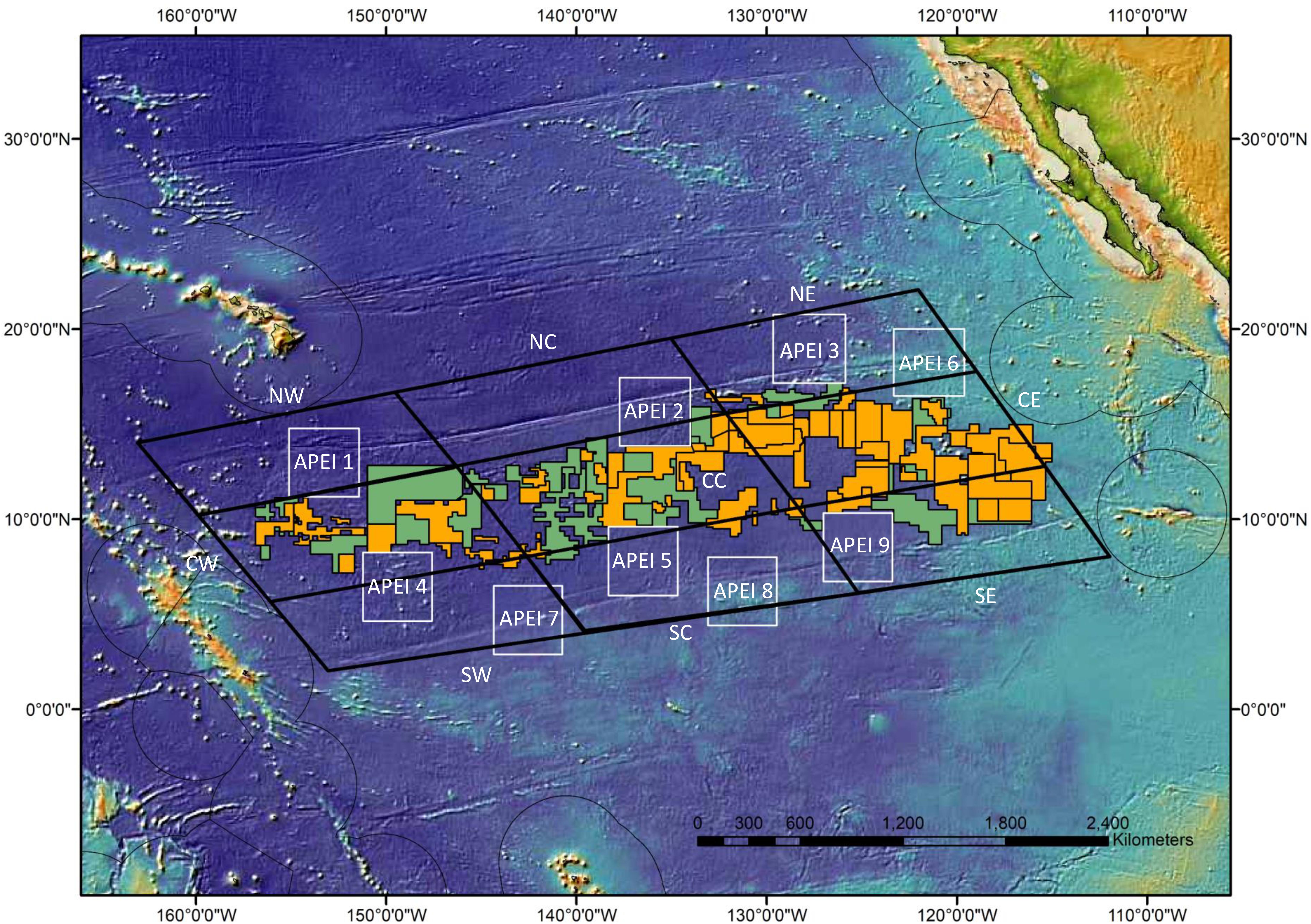
Figure 1. CCZ environmental subregions (large black-outlined parallelograms—NW = northwest, NC = north-central, NE = northeast, CW = central-west, CC = central, CE = central-east, SW = southwest, SC = south-central, and SE = southeast CCZ blocks), exploration areas (orange), reserve areas (green), and APEIs (1–9, outlined in white). APEIs were located by the ISA (2011) to be representative of respective subregions as follows: NE – 1, NC – 2, NE -3, CW – 4, CC – 5, CE – 6, SW – 7, SC – 8, SE – 9. Darker blues represent deeper depths, for values see Supplementary Figure 1.
Data sets for environmental variables compiled for and summarized in the ISA Deep CCZ workshop data report, using measured or modeled values, were collected from online resources and direct solicitations from scientists. All datasets were compiled in ArcGIS 10.7. For display purposes, the values for each variable were divided into ∼5–10 bins to illustrate heterogeneity observed throughout the CCZ. To interpolate point data throughout the CCZ, Empirical Bayesian Kriging was performed in ArcGIS using the empirical transformation and Bessel semi-variogram. All data sets in this study are based on interpolated values, with those not based on satellite data likely interpolated from a limited number of data points. Data sets were analyzed to estimate means, standard deviations, minimum and maximum values for each subregion and APEI (Figure 1).
Seafloor depth data were obtained from ETOPO1 for the grid calculated at 1 arc-minute intervals (Amante and Eakins, 2009; NOAA National Geophysical Data Center, 2009)2 and extracted at 0.5-degree intervals. Means and standard deviations of depths within each subregion and APEI were calculated. Some depth points in a given region, subregion, or APEI may represent seamounts vs. abyssal seafloor; however, owing to the large number of data points and relatively few seamounts, this would be unlikely to skew mean depths. Seamount and knoll data at a resolution of 30 arc-seconds were obtained from Yesson et al. (2011). Seamounts are defined as features rising >1,000 m above the surrounding seafloor, while knolls are defined as features rising between 200 and 1,000 m. Seafloor slope data at a resolution of 1 arc-minute were obtained from McQuaid et al. (2020) who derived slope from the GEneral Bathymetric Chart of the Oceans (GEBCO) bathymetry using the Benthic Terrain Modeler extension in ArcMap 10.4 to determine the largest change in elevation between a cell and its eight nearest neighbors at a scale of 1 km2. Interpolated seafloor slope data were extracted at 1-degree intervals.
Most data for nodule abundance (kg/m2), as well as percent cobalt, nickel, manganese, and copper content of nodules, were obtained from ISA Technical Study No. 6 (ISA, 2012). Nodule abundance data were available between 5.5–19°N and 119–160°W, Co-content data between 5.5–17.5°N and 114–160°W, and other nodule content data between 3–19°N and 115–160°W. Additional unpublished data for all nodule variables, compiled in 2018 were from the area delimited by 2.5–21°N and 112–160°W, excluding contractor areas (see data in Supplementary Material: Dr. C. Morgan, unpublished data). Finally, nodule data were unavailable from the northern 5% of the NE subregion, the western 11% of the NW subregion, and southern 1% of SW subregion as well as several contractor regions in the eastern CE and SE subregions (Figure 1 and Supplementary Figures 5–9). All nodule data were in the form of point values in a 0.5-degree grid. For mapping, values of nodule variables were interpolated as described above.
Sediment type, calcium-carbonate content, and biogenic-silica content were obtained from GeoMapApp,3 and were based on sediment-type analyses of Dutkiewicz et al. (2015), the sediment calcium-carbonate compilation of Archer (2003), and the sediment biogenic-silica (opal) content compilation of Archer (1999). Raw data for sediment type were not available with specific spatial coordinates, so summaries were made based on the figures created in GeoMapApp. Raw sediment calcium carbonate and biogenic silica data were used to interpolate these variables across the entire region, and data were extracted from these interpolations at 1-degree intervals. Sediment total-organic-carbon data were obtained from Jahnke (1996) who digitized Total Organic Carbon (TOC) from Premuzic et al. (1982) at a 2-degree scale. Sediment accumulation-rate data were obtained from Jahnke (1996), who digitized accumulation rates from Cwienk (1986) at a 2-degree scale. Sediment thickness data were obtained from NOAA’s National Centers of Environmental Information4 (Straume et al., 2019). Sediment thickness data extracted at 1-degree intervals were used for calculations of summary statistics.
Bottom-water temperature, salinity, dissolved oxygen concentration, nitrate, phosphate, and silicate data were obtained from NOAA’s Ocean Climate Laboratory Team in the World Ocean Atlas 2018 (WOA18).5 The deepest value for each point below 3,000 m was used as representative of “bottom water,” although data were only available to a depth of 5,500 m. Bottom-water temperature (Locarnini et al., 2019) and salinity (Zweng et al., 2019) data were averaged from 2005 to 2017 and analyzed at 15-arc-minute intervals. Bottom-water concentrations of oxygen, nitrate, phosphate, and silicate were averaged from 1960 to 2017 and calculations of summary statistics were made at 1-degree intervals (Garcia et al., 2019). Bottom-water pH was obtained from Sweetman et al. (2017) who used the program CO2SYS and inorganic CO2, alkalinity, temperature, salinity, and pressure data from the Global Ocean Data Analysis Project and WOA 2013 average from 1998 to 2010 to estimate pH. Calculations on pH data were performed at 0.5-degree intervals. Concentrations of particulate matter in bottom water (1 value 10–15 mab) and nepheloid layer thickness were obtained from Gardner et al. (2018). The nepheloid layer thickness was defined as the distance between the seafloor and sampling depth with a particulate concentration >20 μg/L, with sampling intervals of ∼30 m. Analyses of bottom-water particulate matter concentration and nepheloid-layer thickness data were performed at 1-degree intervals. Bottom-water calcite saturation (1951–2000) was obtained from Levin et al. (2020) at a 0.5-degree scale, and calcite saturation horizon depth was estimated using maps from Yool et al. (2013).
Net Primary Production (NPP) data were obtained from Ocean Productivity website.6 This website provides NPP based on three models: (1) Behrenfeld and Falkowski (1997), the Vertically Generalized Production Model (VGPM), (2) Behrenfeld et al. (2005), the Carbon-based Productivity Model (CBPM), and (3) Silsbe et al. (2016), the Carbon, Absorption, and Fluorescence Euphotic-resolving Model (CAFE). These models all used MODerate resolution Imaging and Spectroradiometer (MODIS) and Sea-viewing Wide Field-of-view Sensor (SeaWiFS) data as well as euphotic zone depth estimates from a model by Morel and Berthon (1989). The NPP data used here represent daily measurements averaged from 1998 to 2010 and 2010 to 2017. NPP data for the 1998–2010 time interval were used to match the interval of analyses performed previously to calculate POC flux using models from Lutz et al. (2007) by Sweetman et al. (2017), while NPP data for the 2010–2017 time interval were used to compare to NPP from the 1998–2010 dataset to examine temporal differences in patterns of surface production throughout the CCZ.
Estimated annual POC flux data to the seafloor were obtained from Lutz et al. (2007), hereafter named Lutz POC, who used 8-day SeaWiFS satellite images of chlorophyll-a concentrations (1997–2004), VGPM NPP, and ETOPO1 data to estimate seafloor flux. Comparisons were also made to estimated annual POC flux data obtained from Sweetman et al. (2017), who used monthly SeaWiFS (1998–2007) and MODIS (2008–2010) chlorophyll-a concentrations, VGPM NPP, and ETOPO1 data to estimate seafloor flux with the flux model created by Lutz et al. (2007).
Projected changes in bottom-water temperature, oxygen, pH, POC flux, and calcite saturation (from 1951–2000 to 2081–2100), were obtained from Levin et al. (2020). All projections are based on the Representative Concentration Pathway (RCP) 8.5 climate-change scenario, and projected values (2081–2100) were subtracted from historical values (1951–2000) to get change over time. Model results were mapped at a 0.5-degree resolution using bilinear interpolation.
Lower-bathyal (800–3,500 m) and abyssal (3,500–6,500 m) biogeographic province boundaries were obtained from Watling et al. (2013), who used environmental variables as proxies to postulate the distribution of deep-sea biogeographic provinces. Seamount biogeographical classifications were obtained from Clark et al. (2010), who refined abyssal biogeographic province boundaries from UNESCO (2009). Pelagic marine provinces were obtained from UNESCO (2009).
Data for all compiled environmental variables were extracted for each CCZ subregion as well as for each APEI at the spatial resolution provided in the data sources as indicated above. If the data sources were only provided as spatial rasters, then data were extracted at 1-degree intervals for our analyses. The mean, minimum, maximum, and range of values within a subregion or APEI for each variable were calculated using R version 4.0. The identification of APEIs and CCZ subregions are given in Figure 1.
Abyssal seafloor depths at 0.5-degree resolution increase from east to west and south to north within the CCZ (Table 1 and Supplementary Figure 1), yielding shallowest average abyssal depths (∼4,300–4,500 m) in the southeast and central-east near the fracture zones, and deepest average depths (∼5,400 m) in the northwest (south of Hawaii). The central CCZ has the smallest range in abyssal seafloor depths (∼4,650–5,350 m) while the northern areas near, the Clarion Fracture Zone, have the largest range (∼3,900–5,800 m), although this range could include seamounts. The APEIs have similar depths to their designated subregions, except for APEIs 5 and 6, which are substantially shallower than their subregions (CC and CE, respectively). The greatest average depths are found in APEI 1 (∼5,400 m) (Table 1 and Supplementary Figure 1). No APEI has a depth range, at 0.5-degree resolution, greater than 1,000 m.
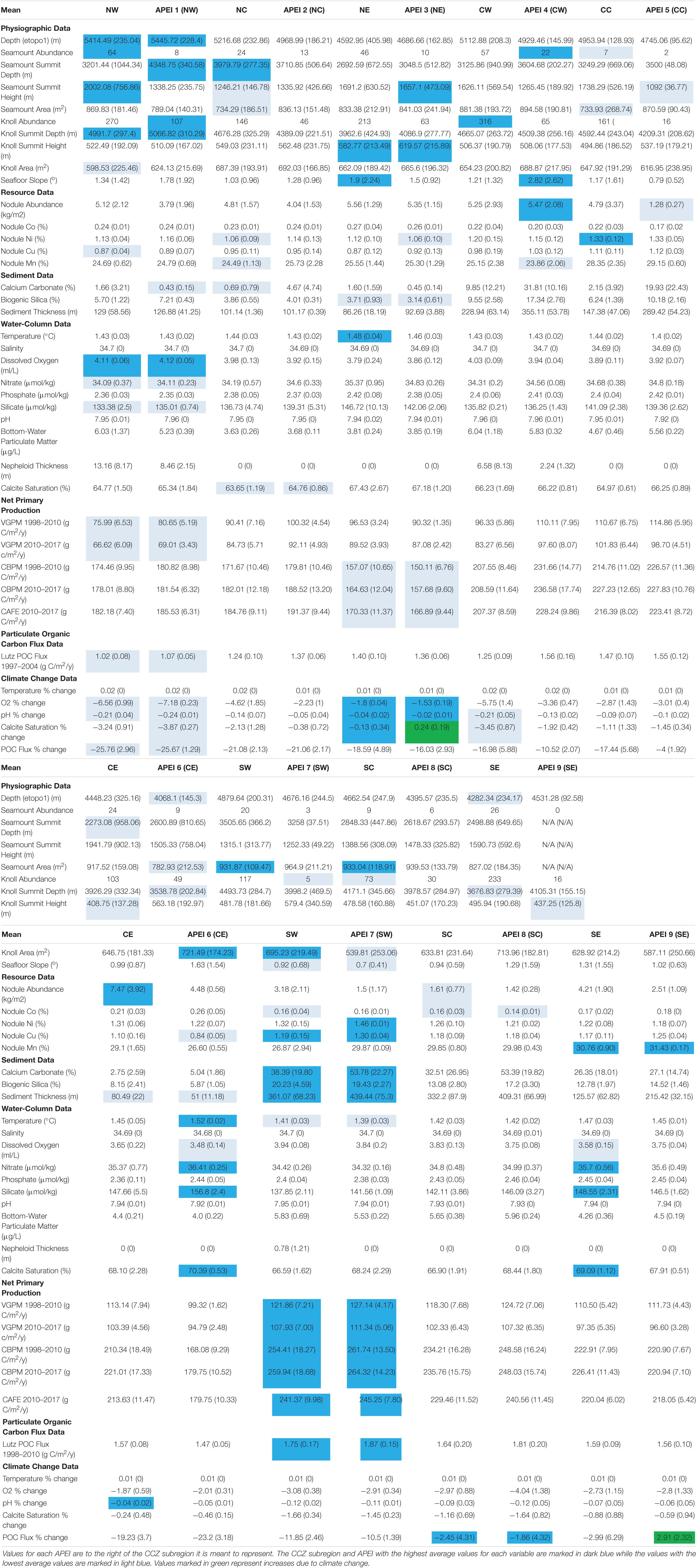
Table 1. The mean (standard deviation) of environmental variables in each CCZ subregion and APEI.
Based on bathymetry at 30 arc-second resolution (Yesson et al., 2011), there were 347 seamounts (elevation >1,000 m) within the CCZ. These were distributed primarily around the fracture zones and at the eastern and western ends of the CCZ, including the peripheral exploration claim areas and APEIs, with the western CCZ having the highest abundance (Table 1 and Supplementary Figure 2). APEI 9 has no seamounts, the majority of APEIs have <10, and APEI 4 had the highest number (22) (Supplementary Table 1 and Supplementary Figure 2).
Average seamount summit water depth is shallowest in the east and deepest in the north, corresponding to patterns in seafloor depth (Table 1 and Supplementary Figure 3). The central CCZ contained seamounts of similar summit water depths while the average depth of seamounts in the north ranged from 3,000 to 4,000 m. The average height (from base to summit) of seamounts was highest in the NW and CE (∼2,000 m). The tallest seamounts were >3,500 m tall and found in the north and east (Supplementary Table 1 and Supplementary Figure 4). Most regions had a wide range of seamount heights. Average seamount area was smallest in the central CCZ and largest in the south. The seamounts with smallest areas were in the north, resulting in larger ranges of seamount size here (Supplementary Table 1 and Supplementary Figure 5).
Average seamount summit water depth was lowest in APEIs 6 and 8 (∼2,600 m) and highest in APEI 1 (∼4,300 m) (Table 1 and Supplementary Figure 3). APEI 6 had at least one seamount that reaches 500 m depth, which was much shallower than any seamounts found throughout the rest of the APEI system (Supplementary Table 1). The average height of seamounts was lowest in APEI 5 (∼1,100 m) and highest in APEI 3 (∼1,700 m) (Table 1 and Supplementary Figure 4). Seamounts had smaller average areas in northern APEIs and larger areas in southern APEIs (Supplementary Table 1 and Supplementary Figure 5).
Based on bathymetry at 30 arc-second resolution (Yesson et al., 2011), knolls, with heights of 200–1,000 m above the general seafloor, were much more widely distributed than seamounts, and were common around the periphery of the CCZ. The SC region had the fewest number of knolls, while the most were found in the north and west (Table 1 and Supplementary Figure 6). Subregions with the deepest and shallowest knolls mirrored average depth patterns (Supplementary Figure 7). Knolls were, on average, highest in the NE (∼ 600 m) and lowest in the CE (∼400 m) (Table 1 and Supplementary Figure 8). Average knoll area was highest in the SW (∼700 m2) and lowest in the NW (∼600 m2) (Table 1 and Supplementary Figure 9).
In the APEI system, there were fewer knolls in the southern APEIs and more in the west (Table 1 and Supplementary Figure 6). Average knoll summit depth was lowest in APEI 6 (∼3,500 m) and highest in APEI 1 (∼5,100 m) (Table 1 and Supplementary Figure 7). Average knoll height was lowest in APEI 9 (∼400 m) and highest in APEI 3 (∼600 m) (Table 1 and Supplementary Figure 8). Average knoll area was lowest in APEI 7 (∼500 m2) and highest in APEI 6 (∼700 m2) (Table 1 and Supplementary Figure 9).
High resolution multibeam bathymetry indicates that the seafloor of the CCZ is characterized by ridges and valleys varying in depth by at least 500 m (e.g., Amon et al., 2016), likely resulting from horst and graben structures formed during seafloor spreading (Johnson, 1972; Macdonald et al., 1996). However, these features are poorly resolved in the 0.5-degree bathymetric data available across the CCZ (Supplementary Figure 1). At the 0.5-degree scale, average seafloor slope is generally between 1 and 2 degrees for CCZ subregions and APEIs (Table 1). The highest and most variable slopes are found in the CC and NE (ranging ∼12–13 degrees) (Supplementary Table 1 and Supplementary Figure 10). The high slopes broadly reflect the location of the fracture zones and the seamount/knoll features. Patterns of slopes in APEIs are broadly representative of their respective subregions (Supplementary Figure 10).
Mean nodule abundance in the CCZ at a resolution of 0.5 degrees is highly variable, with some areas completely devoid of nodules while others have nodule densities >18 kg/m2 (ISA, 2012; Supplementary Table 1 and Supplementary Figure 11). Nodule abundance varies over scales of <1 to 100 km apparently related to differences in sedimentation rates, organic matter content, concentration of leachable manganese, and oxygen penetration depth (Mewes et al., 2014). Mean nodule abundances were highest in the CE subregion (∼7.5 kg/m2) and lowest in the southern subregions (∼1.5–3 kg/m2). APEIs 1, 2, 3, 7, 8, and 9 contained lower mean abundance of nodules than their corresponding CCZ subregions (<2 kg/m2 less) (Table 1 and Supplementary Figure 11). APEIs 5 and 6, which were relocated from within their subregions by the ISA (Wedding et al., 2013), have substantially lower mean nodule abundances than their respective subregions (CC and CE; ≥3 kg/m2 less). No APEI contained areas with nodule abundances >9 kg/m2 (Supplementary Table 1). It should be emphasized that these values are from modeled data with a resolution of 0.5 degrees. Core sampling and photograph surveys indicate substantial finer-scale variations in nodule abundance than captured here (e.g., Peukert et al., 2018; Simon-Lledó et al., 2019a).
Mean nodule cobalt content at a resolution of 0.5 degrees was highest in the north (∼0.25%) and lowest in the south (∼0.15%). Cobalt values were very similar between all subregions and APEIs (within 0.02%) except for the CC, where cobalt content was 0.05% higher than in its corresponding APEI (Table 1 and Supplementary Figure 12). Minimum cobalt content was lower and maximum content higher in every subregion vs. nearest APEI (differing by as much as 0.1%) except for APEI 6 (Supplementary Table 1 and Supplementary Figure 12), suggesting that there is variability in nodule composition within CCZ subregions not captured in the APEI system.
In contrast to cobalt, mean nodule nickel content at a resolution of 0.5 degrees was lowest in the north (∼1.1%) and higher in the central and west (∼1.2–1.3%) (Table 1 and Supplementary Figure 13). Nickel content was generally similar between CCZ subregions and corresponding APEIs (within 0.01%), but several subregions had lower minimum and higher maximum nickel values (Supplementary Table 1 and Supplementary Figure 13).
Mean nodule copper content at a resolution of 0.5 degrees increased from north to south (∼0.3–0.4%) and from west to east (∼0.1%). Copper content was also generally similar between CCZ subregions and corresponding APEIs (within 0.05%, although there is a difference of ∼0.25% between CE and APEI 6) (Table 1 and Supplementary Figure 14); however, subregions in the south and west had maximum copper content ∼0.1–0.2% higher than any areas found in the APEI system (Supplementary Table 1 and Supplementary Figure 4).
Mean nodule manganese content at a resolution of 0.5 degrees increased from north to south (∼5–6% increase) and from west to east (∼4–5%), following the same trend as copper. Manganese content was generally similar (i.e., within 1%) between CCZ subregions and corresponding APEIs; however, in the central CCZ, where exploration contract areas are concentrated, maximum manganese values were several percent higher in subregions than in the nearest APEIs (Table 1 and Supplementary Figure 15). Likewise, minimum manganese values were often much lower in subregions than nearby APEIs (as much as 10% between SW and APEI 7), suggesting that there is variation in nodule characteristics and, potentially, habitat structure not captured by the APEI system (Supplementary Table 1 and Supplementary Figure 15).
According to Dutkiewicz et al. (2015), most of the northern and central CCZ is dominated by siliciclastic clay while the southern CCZ is dominated by biogenic calcareous oozes (Supplementary Figure 16). The NW and CW subregions have large areas of radiolarian ooze while much of the SC is comprised of fine-grained calcareous sediment. APEIs generally mirror regional sediment patterns, although much of APEI 6 is indicated to include gravel and coarser siliciclastic material; the only location in the CCZ indicated to have this sediment type (Dutkiewicz et al., 2015; Supplementary Figure 16). However, direct sampling and extensive seafloor photography in APEI 6 primarily found brown-clay sediments (Menendez et al., 2019; Simon-Lledó et al., 2019a).
Total organic carbon content at a 2-degree resolution appeared to be below 0.3% in sediment throughout the CCZ, including within APEIs, with the north having lower TOC than the south (Jahnke, 1996, Plate 2).
Mean calcium-carbonate content at a 1-degree resolution was lowest in the northern (<1–2%) and highest in the southern CCZ (as high as >75%) (Supplementary Figure 17). This is likely related partially to depth, because many of the northern areas tend to be deeper than the calcite compensation depth in the region (∼4,500 m) (Van Andel, 1975). Overlying productivity and sinking calcium carbonate flux most likely also play a role, since areas deeper than 4,500 m in the southern subregions still have moderate calcium carbonate content (10–20%). Sediment calcium-carbonate content varied between several CCZ subregions and corresponding APEIs by as much as 20% (Table 1 and Supplementary Figure 17).
Mean sediment biogenic silica content at a 1-degree resolution appeared to increase from north (3–5%) to south, up to 25–30% in the SW subregion (Table 1 and Supplementary Figure 18). Because of the extremely low number of values collected, including several APEIs with no biogenic silica values, other patterns and comparisons between subregions and APEIs are not appropriate.
Mean sediment thickness at a 1-degree resolution was highest in the SW (∼350 m) and lowest in the northeast (∼100 m), decreasing northward and eastward. Average thickness was generally similar between CCZ subregions and APEIs, although APEIs 4 and 5 differed from their respective subregions (CW and CC) (Table 1 and Supplementary Figure 19).
Sediment accumulation rates at a 2-degree resolution appeared to be below 0.5 g/cm2/1,000 year in nearly all areas of the CCZ seafloor, with the north and central areas having lower sedimentation rates than the south and west (Jahnke, 1996).
At a resolution of 0.25 degrees, mean bottom-water temperature was nearly uniform throughout the CCZ. Nowhere did temperatures fall below 1.3 or rise above 2°C (Table 1 and Supplementary Figure 20). In the west and CE, temperatures varied by ∼0.5–0.6°C, while within all other subregions and all APEIs, temperature variations did not exceed 0.3°C (Supplementary Table 1 and Supplementary Figure 20).
At a resolution of 0.25 degrees, variations in bottom-water salinity were small throughout the CCZ subregions and APEIs, ranging from 34.68 to 34.70 (Table 1 and Supplementary Figure 21).
At a resolution of 1 degree, mean bottom-water oxygen concentrations were lowest in the SE (∼3.6 mL/kg) and highest in the NW (∼4.1 mL/L), decreasing eastward (by ∼0.4 μmol/L) and southward (by ∼0.2 μmol/L) (Table 1 and Supplementary Figure 22). Oxygen concentrations did not fall below 3.2 mL/L throughout the CCZ while maximum oxygen concentrations did not exceed 4.3 mL/L. In the NE CCZ, oxygen concentrations varied by ∼1 mL/L while other areas had less variability. The APEIs had similar oxygen concentrations to adjacent subregions, although oxygen ranges were usually smaller (Supplementary Table 1 and Supplementary Figure 22). Oxygen concentrations seemed to follow similar patterns to seafloor POC flux and organic carbon content, with increases in seafloor POC flux likely resulting in decreases in oxygen due to greater biological oxygen demand. No seafloor areas (bottom waters) in the CCZ had oxygen levels below 3 mL/L, i.e., they remained well above thresholds considered stressful for deep-sea biota (Levin, 2003).
At a resolution of 1 degree, mean bottom-water nitrate concentrations were highest in the SE (∼36 μmol/kg) and lowest in the NW (∼34 μmol/kg), with slight increases moving south (increasing ∼0.5 μmol/kg) and east (∼1 μmol/kg). Average nitrate concentrations in APEIs were similar to their respective subregions (generally differing by less than 0.5 μmol/kg) (Table 1 and Supplementary Figure 23). Minimum nitrate concentrations in APEIs were somewhat higher than their respective subregions, although all values were within 2 μmol/kg (Supplementary Table 1 and Supplementary Figure 23).
Mean bottom-water phosphate concentrations at a 1-degree resolution were relatively uniform throughout the CCZ, with all average values near 2.4 μmol/kg (Table 1 and Supplementary Figure 24). The NE and CE varied by 0.5 μmol/kg, twice the variability of any other area (Supplementary Table 1 and Supplementary Figure 24).
Mean bottom-water silicate concentrations at a 1-degree resolution were highest in the SE (∼157 μmol/kg) and lowest in the NW (∼133 μmol/kg), generally increasing from north to south and west to east. While CCZ subregions and corresponding APEIs had similar average silicate concentrations (with differences generally less than 4 μmol/kg, except between CE and APEI 6), APEIs often had higher minimum values (by ∼5–10 μmol/kg) (Table 1 and Supplementary Figure 25). APEI 6 had higher concentrations than anywhere else, and minimum values (∼152 μmol/kg) here were higher than maximums found in most other areas (Supplementary Table 1 and Supplementary Figure 25).
Mean bottom-water pH at a 0.5-degree resolution was nearly constant throughout the CCZ and APEI system, with average, minimum, and maximum pH falling between 7.9 and 7.98 (Table 1 and Supplementary Figure 26).
Bottom-water particulate matter concentrations at a 1-degree resolution were extremely low in all regions of the CCZ, with means, minimums, and maximums all <10 μg/L, which is below the detectable limit for the methods (Table 1, Supplementary Table 1 and Supplementary Figure 27). These very low values indicate little or no sediment resuspension in the region (Gardner et al., 2018).
There was no evidence of “strong” nepheloid layers in the CCZ, at a 1-degree resolution, with mean, minimum, and maximum thicknesses all <50 m, i.e., below the detectable limit for the methods used (Table 1, Supplementary Table 1 and Supplementary Figure 28). These low values provide no evidence of “strong” nepheloid layers in the region (Gardner et al., 2018).
Bottom waters throughout the region were undersaturated with calcite, with mean calcite saturation at a 0.5-degree resolution lowest in the NC (∼64%) and highest in the CE (∼69%), increasing from north to south (by ∼2–3%) and west to east (by ∼2–3%) (Table 1 and Supplementary Figure 29). Calcite saturation did not fall below 60% throughout the CCZ while it exceeded 70% in areas throughout the south and east (Supplementary Table 1 and Supplementary Figure 29). Saturation levels differed by ≤2% between each subregion and its representative APEI and varied ∼10% within several subregions.
Calcite saturation horizons appear to be above 3 km depth in all areas throughout the CCZ (Yool et al., 2013).
Average, minimum, and maximum NPP estimated by the VGPM model (Behrenfeld and Falkowski, 1997) were highest in the SW (∼110–120 g C/m2/year) and lowest in the NW (∼65–75 g C/m2/year) for both time periods examined (1998–2010 and 2010–2017). NPP increased eastward (by ∼20 g C/m2/year) and southward (by ∼20–50 g C/m2/year) across the CCZ for both time periods (1998–2010 and 2010–2017). NPP was relatively high along the southern CCZ, and there was also a band of higher primary production in the CC and CE subregions (Table 1 and Supplementary Figures 30, 31). NPP was lower in 2010–2017 than 1998–2010 across all subregions; however, relative productivity patterns across the CCZ remained similar (Table 1 and Supplementary Figures 30, 31). The minimum values of ∼55–60 g C/m2/year in the NW were less than half of the maximum values of ∼ 125–135 in the SW. The NE had less spatial variability in NPP than other areas. NPP in APEIs also increased southward, with the highest values in APEIs 7 and 8 (∼125 and 110 g C/m2/year, respectively) (Table 1 and Supplementary Figures 30, 31). Central and western APEIs also had higher NPP than corresponding subregions, while the opposite was true for eastern APEIs.
Average, minimum, and maximum values of NPP estimated via CBPM and CAFE were roughly twice those estimated via the VGPM model (Behrenfeld and Falkowski, 1997). Mean NPP values for CBPM and CAFE NPP were within 5% of each other in nearly all areas, and means ranged between ∼150 and 170 g C/m2/year in the NE to ∼240–260 g C/m2/year in the SW (Table 1 and Supplementary Figures 32–34). Patterns in NPP across the CCZ were also slightly different between the CBPM/CAFE and VGPM models, with CBPM/CAFE showing the lowest values in the NE instead of NW. Comparing time periods, VGPM NPP was always higher in 1998–2010 compared to 2010–2017 while CBPM NPP was always higher in 2010–2017 compared to 1998–2010 (Table 1 and Supplementary Figures 30–33). However, CBPM estimates were more variable than VGPM estimates in 2010–2017 (often 2.3–2.5× greater) compared to 1998–2010 (no more than 2–2.2× greater) illustrating that temporal variability may not be captured the same way among models (Table 1). Another confounding factor is that chlorophyll data used to estimate NPP was estimated using measurements from the SeaWiFs instrument up to the mid-2000s but by MODIS beyond that. Thus, while patterns in NPP across CCZ areas and APEIs are similar among the three different methods with the north and west areas having lower NPP and the south and east areas having higher NPP, the ranking of specific areas is not identical nor are differences among time periods proportional.
Average Lutz POC flux mirrored NPP (measured by VGPM, which was used as an input for POC flux calculations), with lowest mean value in the NW subregion (∼1 g C/m2/year) and highest mean value in the SW subregion (1.74 g C/m2/year) (Table 1 and Supplementary Figure 35). The lowest average Lutz POC flux for APEIs was in APEI 1 (1.07) while the highest average values were in APEIs 7 and 8 (1.8–1.9) which conformed with patterns in CCZ subregions. The NW subregion and APEI 1 were the only areas with POC flux <1 g C/m2/year, while the NE, SW, and SC subregions had flux of ∼2 g C/m2/year in some areas (Supplementary Table 1). Variations in POC fluxes were 2–3 times larger in southern areas compared to the rest of the CCZ except for the NE. When comparing POC data from 1997 to 2004 (Lutz et al., 2007) to data from 1998 to 2010 (Sweetman et al., 2017) mean values for each CCZ subregion and APEI were within 0.01 g C/m2/year between the two time periods. Maximum and minimum Lutz POC flux values were <0.05 g C/m2/year different in the NW, NC, CW, and CC subregions and corresponding APEIs and 0.05–0.1 different in the CE, SW, SC, and SE subregions and corresponding APEIs while maximums were 0.7 and 0.2 g higher in the Lutz et al. (2007) dataset compared to the Sweetman et al. (2017) dataset in the NE and APEI 3 (Supplementary Table 1).
Mean bottom-water temperature at a 0.5-degree resolution is projected to change very little by 2081–2100, with all areas throughout the CCZ seeing less than 0.05% change in absolute temperature (Table 1 and Supplementary Figure 36). The northwest may include areas with slightly more temperature change (0.03%) than the rest of the CCZ (≤0.02%) (Supplementary Table 1 and Supplementary Figure 36).
Mean bottom-water oxygen at a 0.5-degree resolution is projected to change most in the northern and western CCZ, decreasing by ∼5–7% (∼0.25 mL/L), but less change will be observed in the east, decreasing by ∼ 2–3% (∼0.05 mL/L) (Table 1 and Supplementary Figure 37). The NC and CW subregions include areas that may experience ∼3–4% (∼0.1 mL/L) greater decreases in oxygen concentrations compared to their respective APEIs (Supplementary Table 1 and Supplementary Figure 37), although all locations within the CCZ are projected to remain well above oxygen thresholds considered stressful for deep-sea communities (Levin et al., 2009).
Bottom-water pH at a 0.5-degree resolution is projected to change very little by 2100, with the largest decreases of ∼0.2% (0.02 pH units) observed in the NW (Table 1 and Supplementary Figure 38).
Projected bottom-water calcite saturation changes at a 0.5-degree resolution follow the same patterns as bottom-water oxygen and pH, with the largest decreases of ∼2–4% in the north and west, and the smallest decreases in the east at <1% (Table 1 and Supplementary Figure 39). Several subregions include areas that may experience decreases in calcite saturation 1% greater than their corresponding APEIs (Supplementary Table 1 and Supplementary Figure 39). No areas will go from saturated to unsaturated states.
Mean POC Flux to the seafloor at a 0.5-degree resolution is modeled to change much more by 2100 than other variables examined, although patterns of change match the other variables examined above. The largest differences in POC flux are estimated to be in the north where flux may decrease as much as 20–25% (∼0.25–0.35 g C/m2/year), although central subregions may also see a decrease of 15–20% (∼0.25–0.35 g C/m2/year). In contrast, seafloor POC flux in the southeast is estimated to decrease by 2–3% (<0.1 g C/m2/year) and flux is projected to increase in APEI 9 (Table 1 and Supplementary Figure 40). POC flux is projected to change by similar quantities between CCZ subregions and APEIs, except that APEIs 4 and 5 may be less impacted by future changes than their respective subregions, CW and CC. While the southern CCZ as a whole may be less impacted by climate change influences on seafloor POC flux, there are still locations in all 3 southern subregions that are projected to experience POC flux decreases of 10–20% (∼0.4–0.6 g C/m2/year). There are also areas in the SC and SE that are projected to experience POC flux increases of ∼5% (∼0.1 g C/m2/year) (Supplementary Table 1 and Supplementary Figure 40).
The northern and CW subregions of the CCZ are almost entirely within Abyssal Province 12, while the southern, CC, and CE subregions are almost entirely within Abyssal Province 11 postulated by Watling et al. (2013) (Supplementary Figure 41). Likewise, APEIs 1 and 3 were entirely in Abyssal Province 12, APEIs 5, 7, 8, and 9 were entirely in Abyssal Province 11, while APEIs 2, 4, and 6 span both provinces (Supplementary Figure 41).
Seamounts in the western and central CCZ were within Bathyal Province 14 while seamounts in the eastern CCZ were within Bathyal Province 7 postulated by Watling et al. (2013) (Supplementary Figure 42). Likewise, western and central APEIs were in Bathyal Province 14 while western APEIs were in Bathyal Province 7 (Supplementary Figure 42; Watling et al., 2013).
The northern and central CCZ were within the North Central Pacific Gyre pelagic province with the SW in the Equatorial Pacific province and SE in the Eastern Tropical Pacific province (UNESCO, 2009). Likewise, APEIs 1, 2, 3, and 6 were in the North Central Pacific Gyre, APEIs 4, 5, and 7 were in the Equatorial Pacific, and APEIs 8 and 9 in the Eastern Tropical Pacific (Supplementary Figure 44).
Area of Particular Environmental Interest 1 is similar in most variables considered here to its NW subregion. However, there are many shallow (<3,000 m summit depth, Supplementary Figure 3), tall (>2,000 m summit height, Supplementary Figure 4) seamounts in the northwestern corner with no shallow-tall seamounts protected in APEI 1 (Supplementary Figure 3). Areas of low biogenic silica content (<6%; Supplementary Figure 18), low bottom-water silicate (<130 μmol/kg; Supplementary Figure 25), very low POC flux (< ∼1 g C/m2/year; Supplementary Figure 35), and greater projected changes in future bottom-water/POC flux conditions (Supplementary Figures 36–40) occur in the northwestern corner of the NW subregion but are not captured in APEI 1.
Area of Particular Environmental Interest 2 is largely similar to its NC subregion. However, APEI 2 generally has higher POC fluxes to the seafloor than anywhere in the NC (Supplementary Figure 35). The absence of very low POC flux areas in the APEI could reduce its ecological representativity for this subregion (Smith et al., 2008). APEI 2 is also estimated to be less impacted by climate change than the rest of the NC (Supplementary Figures 36–40).
Area of Particular Environmental Interest 3 is largely similar to its NE subregion. While APEI 3 appears to have less variability in many environmental variables than the NE (e.g., depth, Supplementary Figure 1; POC flux, Supplementary Figure 35), much of this range is captured by APEI 6, which is largely contained within the NE subregion (Figure 1).
Area of Particular Environmental Interest 4, which is largely in the SW subregion (Figure 1), has some dissimilarities to the CW subregion it is meant to represent, including lower maximum nodule abundance, lower nodule cobalt content, and higher estimated primary production and seafloor POC flux. In addition, it does not capture the deepest abyssal areas (<5,200 m, Supplementary Figure 1) nor the shallow (<3,000 m, Supplementary Figure 3), tall (>1,500 m, Supplementary Figure 4) seamounts in the west. Low sediment calcium-carbonate content (<20%, Supplementary Figure 17), biogenic-silica content (<15%, Supplementary Figure 18), sediment thickness (<300 m, Supplementary Figure 19), NPP (Supplementary Figures 30–34), and POC flux (<1.35 g C/m2/year) present throughout much of the CW region are also not represented in APEI 4. The differences in seafloor POC flux between CW and APEI 4 may be ecologically significant (Smith et al., 2008).
Area of Particular Environmental Interest 5, which is almost entirely in the SC subregion (Figure 1), has some dissimilarities to the CC subregion it is intended to represent, including in nodule abundance/characteristics and seafloor POC flux. Relatively deep abyssal seafloor (<4,900 m, Supplementary Figure 1), seamounts (Supplementary Figure 2) and knolls (Supplementary Figure 6) are poorly represented in APEI 5 (although seamounts are also very rare in the CC). In addition, APEI 5 has very low nodule abundance compared to the CC subregion (an average difference of ∼3.5 kg/m2, Supplementary Figure 11). Sediment calcium-carbonate content (Supplementary Figure 17), biogenic silica content (Supplementary Figure 18), sediment thickness (Supplementary Figure 19), and bottom-water calcite saturation (Supplementary Figure 29) are also lower in the CC than APEI 5. Reduced nodule abundance in APEI 5 may yield important ecological differences between APEI 5 and CC (McQuaid et al., 2020).
Area of Particular Environmental Interest 6, which is almost entirely in the NE subregion (Figure 1), differs in nodule abundance/characteristics, sediment/bottom-water characteristics, estimated primary production, and POC flux from the CE subregion, which it is intended to represent. APEI 6 is shallower (<4,200 m, Supplementary Figure 1) than most of the CCZ and has lower sediment calcium-carbonate content (<∼5%, Supplementary Figure 17), biogenic-silica content (<∼7%, Supplementary Figure 18), NPP (Supplementary Figures 30–34), and seafloor POC flux (<1.5 g C/m2/year; Supplementary Figure 35), as well as higher bottom-water nitrate concentrations (>36 μmol/kg; Supplementary Figure 23), bottom-water silicate concentrations (>155 μmol/kg; Supplementary Figure 25), and bottom-water calcite saturation (>70%; Supplementary Figure 29) than most of the CE. APEI 6 also includes lower nodule abundances (<5 kg/m2; Supplementary Figure 11) with lower nickel, copper, and manganese contents (Supplementary Figures 13–15) than most of the CE subregion. While many of the sediment and bottom-water characteristic differences are likely not ecologically significant, the differences in nodule abundance/composition and seafloor POC flux may yield important ecological differences between APEI 6 and the CE subregion (Smith et al., 2008; McQuaid et al., 2020).
Area of Particular Environmental Interest 7 is largely similar to it respective SW subregion. While APEI 7 protects only a few of the seamounts and knolls in SW, many of the others are located in APEI 4 (Supplementary Figures 2, 6). APEI 7 does not capture the higher nodule abundances (Supplementary Figure 11), and lower nodule metal contents (Supplementary Figures 12–15), bottom-water silicate concentrations (Supplementary Figure 25), NPP and seafloor POC flux values (Supplementary Figures 30–35) found in SW, but these are captured in APEI 4, which is largely in this region (Figure 1).
Area of Particular Environmental Interest 8 is largely similar to its SC subregion. While some variability in nodule abundance/characteristics (Supplementary Figures 11–15) and sediment characteristics (Supplementary Figures 16–19) in the SC are not fully captured by APEI 8, they are largely present in APEI 5 which is almost entirely within this region (Figure 1).
Area of Particular Environmental Interest 9 has some dissimilarities with its SE subregion. In particular, shallower depths (<∼4,400 m, Supplementary Figure 1), seamounts (Supplementary Figure 2), most knolls (Supplementary Figure 6), higher nodule abundance (>4 kg/m2, Supplementary Figure 11), lower bottom-water oxygen concentrations (<∼3.7 ml/L, Supplementary Figure 22), and higher bottom-water calcite saturation (>∼69%, Supplementary Figure 29) present in the eastern SE are not captured in APEI 9. While differences in bottom-water characteristics are likely not ecologically significant, the lack of seamounts and low nodule abundances in APEI 9 may yield important ecological differences with most of the SE subregion.
While much of the environmental variability in the northern and southern CCZ appears to be captured in the APEI network, the central and SE CCZ may include areas with seafloor POC flux, nodule abundance, and seamount characteristics not found in the APEIs meant to represent them. To ensure adequate protection of biodiversity in these subregions, additional APEIs may be warranted. For detailed habitat mapping in the CCZ using the environmental data in this paper, as well as identification of potential areas for additional representative APEIs, see McQuaid et al. (2020).
In the deep sea, proposed polymetallic nodule mining activities are likely to harm seafloor ecosystems, including unique habitats such as manganese nodules (Glover and Smith, 2003; Niner et al., 2018; Washburn et al., 2019; Smith et al., 2020). To protect regional biodiversity and ecosystem functions from the nodule-mining impacts in the CCZ, nine APEIs were designated as no-mining areas (Wedding et al., 2013). Thus, for the APEI network to serve its purpose in protecting biodiversity and ecosystem function throughout the CCZ, it must fully capture the full range of habitats and important environmental variables found in the region.
While there were statistically significant differences across the CCZ in every environmental variable examined, it is likely that many of these differences are not ecologically significant, and thus are likely less important for the APEI network to fully represent. Differences in seafloor slope, at a broad scale, (Supplementary Figure 10), sediment thickness (Supplementary Figure 19), bottom-water particulate concentrations, and nepheloid-layer thickness (Supplementary Figures 27, 28) are small or within measurement errors and likely not ecologically significant. Variations in bottom-water temperature, salinity, oxygen concentration nitrate concentration, phosphate concentration, silicate concentration, pH, particulate matter concentration, and calcite saturation (Table 1 and Supplementary Table 1 and Supplementary Figures 20–29) are relatively small and may not be ecologically significant (Levin, 2003), although little work has been done to understand how differences in many of these variables affect abyssal communities.
Several studies, including many in this volume, have found that nodule abundance (Amon et al., 2016; De Smet et al., 2017; Simon-Lledó et al., 2019b, 2020; Washburn et al., 2021) and POC flux to the seafloor (Smith et al., 2008; Bonifácio et al., 2020; Washburn et al., 2021) are major drivers of benthic community abundance, diversity, and composition. Both of these variables vary across the CCZ and between some CCZ subregions and their respective APEIs. Differences between APEIs and their subregions are most pronounced in the central CCZ (Table 1 and Supplementary Figures 11 and 35), where APEIs were located away from nodule-rich areas (Wedding et al., 2013). Nodules provide habitat for apparently nodule-dependent epifauna and infauna (Amon et al., 2016; Vanreusel et al., 2016; Gooday et al., 2017; Simon-Lledó et al., 2019b) as well as metal-cycling bacteria and archaea (Shulse et al., 2016; Molari et al., 2020). Thus, differences in nodule abundance and metal composition (Table 1 and Supplementary Figures 11–15) are likely to be ecological significant. Although seafloor POC flux appears to have large impacts on benthic communities (e.g., Smith et al., 2008), there are relatively few POC flux measurements from the CCZ (Lutz et al., 2007; Kim et al., 2010, 2011, 2012). Therefore, patterns of seafloor POC flux across the CCZ are estimated from models of export through the water column (e.g., Lutz et al., 2007). Substantially more direct measurements of deep POC flux are needed to better understand food availability in space and time across the CCZ.
Seamounts also serve as important habitats for benthic and pelagic communities (Clark et al., 2010; Leitner et al., 2017; Laroche et al., 2020). Seamount and knoll habitats appear to be underrepresented in the APEIs for the central CCZ (Supplementary Figure 2). Other variables with differences that could be ecologically significant include sediment calcium carbonate and biogenic silica content (Table 1 and Supplementary Figures 17, 18), which may influence the formation of molluscan and foraminiferan shells (Wheeler, 1992; Sen Gupta, 1999). Finally, it appears that changes in bottom-water temperature, oxygen content, and pH due to climate change will likely not be ecologically significant throughout the CCZ, while it is unclear whether changes in calcite saturation will be (Supplementary Figures 36–39). However, estimated climate driven changes in POC flux for time intervals 1951–2000 to 2081–2100 between APEIs and their respective subregions may be as much as ∼30% (Supplementary Figure 40), which could significantly influence abyssal benthic communities (Smith et al., 2008; Jones et al., 2013) in the deep-sea throughout the CCZ, albeit unevenly (Supplementary Figure 40).
There is significant heterogeneity in all environmental variables examined across the CCZ. Much of this variability falls along north–south and east–west gradients, as postulated by Wedding et al. (2013). Most of this environmental variability is captured by the APEI system erected by the ISA’s Regional Environmental Management Plan (ISA, 2011), but some APEIs differ in some important ecological characteristics (in particular nodule abundance and seafloor POC flux) from the subregions they were intended to represent, especially the central and SE CCZ. Thus, the formation of additional APEIs or other protected areas merits consideration, particularly within the nodule-rich central areas of the CCZ. Areas where additional APEIs could be erected to help protect some of these habitats are proposed in McQuaid et al. (2020).
The original contributions presented in the study are included in the article/Supplementary Material, further inquiries can be directed to the corresponding author/s.
CRS and TW designed the study while TW accumulated all data sets and wrote the first draft. DJ and C-LW contributed datasets. All authors provided analytical support and revisions.
This work was funded by grants to CRS from the Gordon and Betty Moore Foundation (no. 5596) and the Pew Charitable Trusts (no. 32871).
The authors declare that the research was conducted in the absence of any commercial or financial relationships that could be construed as a potential conflict of interest.
The authors thank the individuals and institutions who collected and/or provided data for this synthesis. In particular, we would like to thank Malcolm Clark for providing seamount and knoll data from Yesson et al. (2011), Kirsty McQuaid for providing seafloor slope data used in McQuaid et al. (2020), Charles Morgan for providing nodule abundance and metal-content data from ISA (2012) and proprietary 2018 data, Wilford Gardner and Alexey Mishonov for providing bottom-water particulate matter and nepheloid layer thickness data from Gardner et al. (2018), Robert O’Malley for assisting with NPP data provision, and Les Watling for providing CCZ ecoregion data. This is publication number 11296 from the School of Ocean and Science and Technology, University of Hawaii.
The Supplementary Material for this article can be found online at: https://www.frontiersin.org/articles/10.3389/fmars.2021.661685/full#supplementary-material
Amante, C., and Eakins, B. W. (2009). ETOPO1 1 Arc-Minute Global Relief Model: Procedures, Data Sources and Analysis. NOAA Technical Memorandum NESDIS NGDC-24. Boulder, CO: National Geophysical Data Center, NOAA, doi: 10.7289/V5C8276M
Amon, D. J., Ziegler, A. F., Dahlgren, T. G., Glover, A. G., Goineau, A., Gooday, A. J., et al. (2016). Insights into the abundance and diversity of abyssal megafauna in a polymetallic-nodule region in the eastern Clarion-Clipperton Zone. Sci. Rep. 6:30492. doi: 10.1038/srep30492
Archer, D. E. (1999). Opal, Quartz and Calcium Carbonate Content in Surface Sediments of the Ocean Floor. Los Angeles, CA: PANGAEA, doi: 10.1594/PANGAEA.56017
Archer, D. E. (2003). Interpolated Calcium Carbonate Content of the Sea Floor Sediments. Los Angeles, CA: PANGAEA, doi: 10.1594/PANGAEA.107286
Behrenfeld, M. J., Boss, E., Siegel, D. A., and Shea, D. M. (2005). Carbon-based ocean productivity and phytoplankton physiology from space. Glob. Biogeochem. Cycles 19, 1–14.
Behrenfeld, M. J., and Falkowski, P. G. (1997). Photosynthetic rates derived from satellite-based chlorophyll concentrations. Limnol. Oceanogr. 42, 1–20. doi: 10.4319/lo.1997.42.1.0001
Bonifácio, P., Martinez-Arbizu, P., and Menot, L. (2020). Alpha and beta diversity patterns of polychaete assemblages across the nodule province of the clarion-clipperton fracture zone (Equatorial Pacific). Biogeosciences 17, 865–886. doi: 10.5194/bg-17-865-2020
Borowski, C., and Thiel, H. (1998). Deep-sea macrofaunal impacts of a large-scale physical disturbance experiment in the Southeast Pacific. Deep Sea Res. II 45, 55–81. doi: 10.1016/s0967-0645(97)00073-8
Clark, M. R., Rowden, A. A., Schlacher, T., Williams, A., Consalvey, M., Stocks, K. I., et al. (2010). The ecology of seamounts: structure, function, and human impacts. Annu. Rev. Mar. Sci. 2, 253–278. doi: 10.1146/annurev-marine-120308-081109
Cwienk, D. S. (1986). Recent and Glacial Age Organic Carbon and Biogenic Silica Accumulation in Marine Sediments. 249. Ph.D. Thesis. University of Rhode Island, Kingston, RI.
Danovaro, R., Snelgrove, P. V. R., and Tyler, P. (2014). Challenging the paradigms of deep-sea ecology. Trends Ecol. Evol. 29, 465–475. doi: 10.1016/j.tree.2014.06.002
De Smet, B., Paper, E., Riehl, T., Bonifácio, P., Colson, L., and Vanreusel, A. (2017). The community structure of deep-sea macrofauna associated with polymetallic nodules in the eastern part of the Clarion Clipperton Fracture Zone. Front. Mar. Sci. 4:103. doi: 10.3389/fmars.2017.00103
Dutkiewicz, A., Muller, R. D., O’Callaghan, S., and Jonasson, H. (2015). Census of seafloor sediments in the world’s ocean. Geology 43, 795–798. doi: 10.1130/g36883.1
Garcia, H. E., Weathers, K. W., Paver, C. R., Smolyar, I., Boyer, T. P., Locarnini, R. A., et al. (2019). World Ocean Atlas 2018: Dissolved Oxygen, Apparent Oxygen Utilization, and Dissolved Oxygen Saturation. NOAA Atlas NESDIS 83, Vol. 3, ed. A. Mishonov (Silver Spring, MA: U.S. Department Of Commerce), 38.
Gardner, W. D., Richardson, M. J., Mishonov, A. V., and Biscaye, P. E. (2018). Global comparison of benthic nepheloid layers based on 52 yeas of nephelometer and transmissometer measurements. Prog. Oceanogr. 168, 100–111. doi: 10.1016/j.pocean.2018.09.008
Glover, A. G., and Smith, C. R. (2003). The deep-sea floor ecosystem: current status and prospects of anthropogenic change by the year 2025. Environ. Conserv. 30, 219–241. doi: 10.1017/S0376892903000225
Gooday, A. J., Holzmann, M., Caulle, C., Goineau, A., Kamenskaya, O., Weber, A. A.-T., et al. (2017). Giant protists (xenophyophores, Foraminifera) are exceptionally diverse in parts of the abyssal eastern Pacific licensed for polymetallic nodule exploration. Biol. Conserv. 107, 106–116. doi: 10.1016/j.biocon.2017.01.006
Hein, J. R., Mizell, K., Koschinsky, A., and Conrad, T. A. (2013). Deep-ocean mineral deposits as a source of critical metals for high- and green-technology applications: comparison with land-based resources. Ore Geol. Rev. 51, 1–14. doi: 10.1016/j.oregeorev.2012.12.001
ISA (2008). Rationale and Recommendations for the Establishment of Preservation Reference Areas for Nodule Mining in the Clarion-Clipperton Zone: Summary Outcomes of a Workshop to Design Marine Protected Areas for Seamounts and the Abyssal Nodule Province in Pacific High Seas, Held at the University of Hawaii at Manoa, Hawaii, United States of America, from 23 to 26 October 2007. ISBA/14/LTC/2. Kingston: International Seabed Authority, 12.
ISA (2011). Environmental Management Plan for the Clarion-Clipperton Zone. ISBA/17/LTC/7. Kingston: International Seabed Authority, 18.
ISA (2012). A Geological Model of Polymetallic Nodule Deposits in the Clarion-Clipperton Fracture Zone. ISA Technical Study No. 6. Kingston: International Seabed Authority, 106.
ISA (2019). Deep CCZ Biodiversity Synthesis Workshop Report. Deep CCZ Biodiversity Synthesis Workshop. Friday Harbor, WA: University of Hawaii at Manoa & International Seabed Authority.
Jahnke, R. A. (1996). The global ocean flux of particulate organic carbon: Areal distribution and magnitude. Glob. Biogeochem. Cycles 10, 71–88. doi: 10.1029/95gb03525
Johnson, D. A. (1972). Ocean-floor erosion in equatorial Pacific. Geol. Soc. Am. Bull. 83, 3121–3144. doi: 10.1130/0016-7606(1972)83[3121:oeitep]2.0.co;2
Jones, D. O. B., Kaiser, S., Sweetman, A. K., Smith, C. R., Menot, L., Vink, A., et al. (2017). Biological responses to disturbance from simulated deep-sea polymetallic nodule mining. PLoS One 12:e171750. doi: 10.1371/journal.pone.0171750
Jones, D. O. B., Yool, A., Wei, C.-L., Henson, S. A., Ruhl, H. A., Watson, R. A., et al. (2013). Global reductions in seafloor biomass in response to climate change. Glob. Change Biol. 20, 1861–1872. doi: 10.1111/gcb.12480
Kim, H. J., Hyeong, K., Yoo, C. M., Chi, S.-B., Khim, B.-K., and Kim, D. (2010). Seasonal variations of particle fluxes in the northeastern equatorial Pacific during normal and weak El Niño periods. Geosci. J. 14, 415–422.
Kim, H. J., Hyeong, K., Yoo, C. M., Khim, B. K., Kim, K. H., Son, J. W., et al. (2012). Impact of strong El Niño events (1997/98 and 2009/10) on sinking particle fluxes in the 10°N thermocline ridge area of the northeastern equatorial Pacific. Deep Sea Res. I Oceanogr. Res. Pap. 67, 111–120.
Kim, H. J., Kim, D., Yoo, C. M., Chi, S.-B., Khim, B. K., Shin, H.-R., et al. (2011). Influence of ENSO variability on sinking-particle fluxes in the northeastern equatorial Pacific. Deep Sea Res. I 58, 865–874. doi: 10.1016/j.dsr.2011.06.007
Laroche, O., Kersten, O., Smith, C. R., and Goetze, E. (2020). Environmental DNA surveys detect distinct metazoan communities across abyssal plains and seamounts in the western Clarion Clipperton Zone. Mol. Ecol. 29, 4588–4604. doi: 10.1111/mec.15484
Leitner, A. B., Neuheimer, A. B., Donlon, E., Smith, C. R., and Drazen, J. C. (2017). Environmental and bathymetric influences on abyssal bait-attending communities of the Clarion Clipperton Zone. Deep Sea Res. I 125, 65–80. doi: 10.1016/j.dsr.2017.04.017
Levin, L. A., Ekau, W., Gooday, A. J., Jorissen, F., Middelburg, J. J., Naqvi, S. W. A., et al. (2009). Effects of natural and human-induced hypoxia on coastal benthos. Biogeosciences 6, 2063–2098. doi: 10.5194/bg-6-2063-2009
Levin, L., Wei, C.-L., Dunn, D., Amon, D., Ashford, O., Cheung, W., et al. (2020). Climate change considerations are fundamental to management of deep-sea resource extraction. Glob. Change Biol. 26, 4664–4678. doi: 10.1111/gcb.15223
Levin, L. A. (2003). Oxygen minimum zone benthos: adaptation and community response to hypoxia. Oceanogr. Mar. Biol. 41, 1–45.
Locarnini, R. A., Mishonov, A. V., Baranova, O. K., Boyer, T. P., Zweng, M. M., Garcia, H. E., et al. (2019). World Ocean Atlas 2018: Temperature. NOAA Atlas NESDIS 81, Vol. 1, ed. A. Mishonov (Silver Spring, MD: U.S. Department Of Commerce), 52.
Lutz, M. J., Caldeira, K. R., Dunbar, R. B., and Behrenfeld, M. J. (2007). Seasonal rhythms of net primary production and particulate organic carbon flux to depth describe the efficiency of biological pump in the global ocean. J. Geophys. Res. Oceans 112:C10011.
Macdonald, K. C., Fox, P. J., Alexander, R. T., Pockalny, R., and Gente, P. (1996). Volcanic growth faults and the origin of Pacific abyssal hills. Nature 380, 125–129. doi: 10.1038/380125a0
McQuaid, K. A., Attrill, M. J., Clark, M. R., Cobley, A., Glover, A. G., Smith, C. R., et al. (2020). Using habitat classification to assess representativity of a protected area network in a large, data-poor area targeted for deep-sea mining. Front. Mar. Sci. 7:558860. doi: 10.3389/fmars.2020.558860
Menendez, A., James, R. H., Lichtschlag, A., Connelly, D., and Peel, K. (2019). Controls on the chemical composition of ferromanganese nodules in the Clarion-Clipperton Fracture Zone, eastern equatorial Pacific. Mar. Geol. 409, 1–14. doi: 10.1016/j.margeo.2018.12.004
Mewes, K., Mogollón, J. M., Picard, A., Rühlemann, C., Kuhn, T., Nöthen, K., et al. (2014). Impact of depositional and biogeochemical processes on small scale variations in nodule abundance in the Clarion-Clipperton Fracture Zone. Deep Sea Res. I Oceanogr. Res. Pap. 91, 125–141. doi: 10.1016/j.dsr.2014.06.001
Molari, M., Janssen, F., Vonnahme, T. R., Wenzhöfer, F., and Boetius, A. (2020). The contribution of microbial communities in polymetallic nodules to the diversity of the deep-sea microbiome of the Peru Basin (4130-4198 m depth). Biogeosciences 17, 3203–3222. doi: 10.5194/bg-17-3203-2020
Morel, A., and Berthon, J.-F. (1989). Surface pigments, algal biomass profiles, and potential production of the euphotic layer: relationships reinvestigated in view of remote-sensing applications. Limnol. Oceanogr. 34, 1545–1562. doi: 10.4319/lo.1989.34.8.1545
Niner, H. J., Ardron, J. A., Escar, E. G., Gianni, M., Jaeckel, A., Jones, D. O. B., et al. (2018). Deep-sea mining with no net loss of biodiversity – an impossible aim. Front. Mar. Sci. 5:53. doi: 10.3389/fmars.2018.00053
NOAA National Geophysical Data Center (2009). ETOPO1 1 Arc-Minute Global Relief Model. Asheville, NC: NOAA National Centers for Environmental Information.
Peukert, A., Timm, S., Alevizos, E., Köser, K., Kwasnitschka, T., and Greinert, J. (2018). Understanding Mn-nodule distribution and evaluation of related deep-sea mining impacts using AUV-based hydroacoustic and optical data. Biogeosciences 15, 2525–2549. doi: 10.5194/bg-15-2525-2018
Premuzic, E. T., Benkovitz, C. M., Gaffney, J. S., and Walsh, J. J. (1982). The nature and distribution of organic matter in the surface sediments of world oceans and seas. Org. Geochem. 4, 63–77. doi: 10.1016/0146-6380(82)90009-2
Shulse, C. N., Maillot, B., Smith, C. R., and Church, M. J. (2016). Polymetallic nodules, sediments, and deep waters in the equatorial North Pacific exhibit highly diverse and distinct bacterial, archaeal, and microeukaryotic communities. Microbiologyopen 6:e00428. doi: 10.1002/mbo3.428
Silsbe, G. M., Behrenfeld, M. J., Halsey, K. H., Milligan, A. J., and Westberry, T. K. (2016). The CAFE model: a net production model for global ocean phytoplankton. Glob. Biogeochem. Cycles 30, 1756–1777. doi: 10.1002/2016gb005521
Simon-Lledó, E., Bett, B. J., Huvenne, V. A. I., Schoening, T., Benoist, N. M. A., Jeffreys, R. M., et al. (2019a). Megafaunal variation in the abyssal landscape of the Clarion Clipperton Zone. Prog. Oceanogr. 170, 119–133. doi: 10.1016/j.pocean.2018.11.003
Simon-Lledó, E., Bett, B. J., Huvenne, V. A. I., Schoening, T., Benoist, N. M. A., and Jones, D. O. B. (2019b). Ecology of a polymetallic nodule occurrence gradient: implications for deep-sea mining. Limnol. Oceanogr. 64, 1883–1894. doi: 10.1002/lno.11157
Simon-Lledó, E., Pomee, C., Ahokava, A., Drazen, J. C., Leitner, A. B., Flynn, A., et al. (2020). Multi-scale variations in invertebrate and fish megafauna in the mid-eastern Clarion Clipperton Zone. Prog. Oceanogr. 187:102405. doi: 10.1016/j.pocean.2020.102405
Smith, C. R., De Leo, F. C., Bernardino, A. F., Sweetman, A. K., and Arbizu, P. M. (2008). Abyssal food limitation, ecosystem structure and climate change. Trends Ecol. Evol. 23, 518–528. doi: 10.1016/j.tree.2008.05.002
Smith, C. R., Tunnicliffe, V., Colaco, A., Drazen, J. C., Gollner, S., Levin, L. A., et al. (2020). Deep-sea misconceptions cause underestimation of seabed-mining impacts. Trends Ecol. Evol. 35, 853–857. doi: 10.1016/j.tree.2020.07.002
Straume, E. O., Gaina, C., Medvedev, S., Hochmuth, K., Gohl, K., Whittaker, J. M., et al. (2019). GlobSed: updated total sediment thickness in the world’s oceans. Geochem. Geophys. Geosyst. 20, 1756–1772. doi: 10.1029/2018GC008115
Sweetman, A. K., Thurber, A. R., Smith, C. R., Levin, L. A., Mora, C., Wei, C. L., et al. (2017). Major impacts of climate change on deep-sea benthic ecosystems. Elem. Sci. Anth. 5:4. doi: 10.1525/elementa.203
UNESCO (2009). Global Oceans and Deep Seabed – Biogeographic Classification. IOC Technical Series, Vol. 84. Paris: UNESCO-IOC, 87.
Van Andel, T. H. (1975). Mesozoic/Cenozoic calcite compensation depth and the global distribution of calcareous sediments. Earth Planet. Sci. Lett. 26, 187–194. doi: 10.1016/0012-821x(75)90086-2
Vanreusel, A., Hilrio, A., Ribeiro, P. A., Menot, L., and Arbizu, P. M. (2016). Threatened by mining, polymetallic nodules are required to preserve abyssal epifauna. Sci. Rep. 6:26808.
Washburn, T. W., Menot, L., Bonifácio, P., Pape, E., Błazewicz, M., Bribiesca-Contreras, G., et al. (2021). Patterns of macrofaunal biodiversity across the Clarion-Clipperton Zone: an area targeted for seabed mining. Front. Mar. Sci. doi: 10.3389/fmars.2021.626571
Washburn, T. W., Turner, P. J., Durden, J. M., Jones, D. O. B., Weaver, P., and Van Dover, C. L. (2019). Ecological risk assessment for deep-sea mining. Ocean Coast. Manag. 176, 24–39. doi: 10.1016/j.ocecoaman.2019.04.014
Watling, L., Guinotte, J., Clark, M. R., and Smith, C. R. (2013). A proposed biogeography of the deep ocean floor. Prog. Oceanogr. 111, 91–112. doi: 10.1016/j.pocean.2012.11.003
Weaver, P. P. E., Billett, D. S. M., and Van Dover, C. L. (2018). “Environmental risks of deep-sea mining,” in Handbook on Marine Environment Protection, eds M. Salomon and T. Markus (Cham: Spring), doi: 10.1007/978-3-319-60156-4_11
Wedding, L. M., Friedlander, A. M., Kittinger, J. N., Watling, L., Gaines, S. D., Bennett, M., et al. (2013). From principles to practice: a spatial approach to systematic conservation planning in the deep sea. Proc. R. Soc. B 280:20131684. doi: 10.1098/rspb.2013.1684
Wei, C.-L., Rowe, G. T., Escobar-Briones, E., Boetius, A., Soltwedel, T., Caley, M. J., et al. (2010). Global patterns and predictions of seafloor biomass using random forests. PLoS One 5:e15323. doi: 10.1371/journal.pone.0015323
Yesson, C., Clark, M. R., Taylor, M. L., and Rogers, A. D. (2011). The global distribution of seamounts based on 30 arc seconds bathymetry data. Deep Sea Res. I 58, 442–453. doi: 10.1016/j.dsr.2011.02.004
Yool, A., Popova, E. E., and Anderson, T. R. (2013). MEDUSA-2.0: an intermediate complexity biogeochemical model of the marine carbon cycle for climate change and ocean acidification studies. Geosci. Model Dev. Discuss. 6, 1259–1365.
Zeppilli, D., Pusceddu, A., Trincardi, F., and Danovaro, R. (2016). Seafloor heterogeneity influences the biodiversity-ecosystem functioning relationships in the deep sea. Sci. Rep. 6:26352.
Keywords: deep-sea mining, areas of particular environmental interest, environmental heterogeneity, Clarion-Clipperton Zone, manganese nodules, POC flux, sediment characteristics, climate change
Citation: Washburn TW, Jones DOB, Wei C-L and Smith CR (2021) Environmental Heterogeneity Throughout the Clarion-Clipperton Zone and the Potential Representativity of the APEI Network. Front. Mar. Sci. 8:661685. doi: 10.3389/fmars.2021.661685
Received: 31 January 2021; Accepted: 11 March 2021;
Published: 30 March 2021.
Edited by:
Jacopo Aguzzi, Instituto de Ciencias del Mar (CSIC), SpainReviewed by:
Hiroyuki Yamamoto, Japan Agency for Marine-Earth Science and Technology (JAMSTEC), JapanCopyright © 2021 Washburn, Jones, Wei and Smith. This is an open-access article distributed under the terms of the Creative Commons Attribution License (CC BY). The use, distribution or reproduction in other forums is permitted, provided the original author(s) and the copyright owner(s) are credited and that the original publication in this journal is cited, in accordance with accepted academic practice. No use, distribution or reproduction is permitted which does not comply with these terms.
*Correspondence: Travis W. Washburn, VHJhdmlzLldhc2hidXJuQGFpc3QuZ28uanA=
Disclaimer: All claims expressed in this article are solely those of the authors and do not necessarily represent those of their affiliated organizations, or those of the publisher, the editors and the reviewers. Any product that may be evaluated in this article or claim that may be made by its manufacturer is not guaranteed or endorsed by the publisher.
Research integrity at Frontiers
Learn more about the work of our research integrity team to safeguard the quality of each article we publish.