Measurements and Spatial Distribution Simulation of Impact Pile Driving Underwater Noise Generated During the Construction of Offshore Wind Power Plant Off the Southwest Coast of Korea

Offshore wind power plants are under construction worldwide, and concerns about the adverse effects of underwater noise generated during their construction on the marine environment are increasing. As part of an environmental impact assessment, underwater noise generated by impact pile driving was measured during the construction of an offshore wind farm off the southwest coast of Korea. The sound exposure levels of impact pile driving noise were estimated as a function of distance and compared with those predicted by a damped cylindrical spreading model and broadband parabolic equation simulation. Source level at 1 m was estimated to be in a range of 183–184 dB re 1μPa²s in the sound exposure level based on the model predictions and it tended to decrease by 21log⁡r as the distance increased. Finally, the spatial distribution of impact pile driving noise was predicted. This result, if combined with noise-induced damage thresholds for marine life, may be used to assess the effects of wind farm construction on marine ecosystems.

Introduction

As global interest in renewable energy has increased, technologies to exploit wind energy are actively being developed. As onshore wind farms are often accompanied by landscape damage and noise, offshore wind power generation has been considered an attractive alternative. There are several foundation types of offshore wind turbine construction such as monopiles, tripods, steel jackets, suction caisson, gravity-based structure and floating (Sánchez et al., 2019; Tsouvalas, 2020). Among them, processes involving percussive pile driving produce underwater noise with extremely high sound pressure levels. Recently, it has been reported that impact pile driving noise may be responsible for negative effects on marine life, including marine mammals (Nehls et al., 2007; Kastelein et al., 2013; Leunissen and Dawson, 2018; Leunissen et al., 2019) and fish (Nedwell et al., 2003; Casper et al., 2013; Bagocius, 2015; Hawkins and Popper, 2017). Several studies have been conducted to investigate the mechanism of impact pile driving noise and its propagation properties (Reinhall and Dahl, 2011; Tsouvalas, 2020). In addition, there have been efforts to present the standards for measurement, analysis, and prediction of the noise and to prepare the criteria for the assessing noise impacts on marine ecosystems (Oestman et al., 2009; Ainslie, 2011; de Jong et al., 2011; Hawkins and Popper, 2014; Robinson et al., 2014; Dahl et al., 2015; International Organization for Standardization [ISO], 2017b; National Marine Fisheries Service [NMFS], 2018; Southall et al., 2019).

Compressional wave generated by hammer strikes from impact pile driving is Mach wave of which the speed exceeds the sound speed in water (Reinhall and Dahl, 2011). Beginning at the top of the pile, a compressional wave propagates downward with a sound speed c_p, in a conical radiation pattern in water. The launch angle θ_w of the Mach cone is given by Reinhall and Dahl (2011).

${\mathrm{\theta }}_w={\sin }^{-1}\frac{c_w}{c_p},(1)$

where c_w is the sound speed in the water medium. The Mach wave is then reflected from the end of the pile and again from the top of the pile. Additional reflections continue to occur at both ends of the pile. For this reason, the propagation pattern of pile driving noise differs from that of an omnidirectional single-point source. Generally, sound propagation in water is a function of distance, with a form of Nlog⁡r, where r is the distance in meters from a sound source and N is a spreading constant that depends on the ocean environment; for example, 10log⁡r for cylindrical spreading in shallow water and 20log⁡r for spherical spreading in deep water (Jensen et al., 2011). However, this simple formula does not consider range-dependent ocean environments and the geoacoustic properties of sediment, which can have a strong influence on sound propagation in ocean waveguides.

Several efforts have been made to predict the propagation of the impact pile driving noise (e.g., Workshop COMPILE I and II). First-generation models using parabolic equation (PE), normal mode, wavenumber integration and energy flux-based methods for long-range propagation and finite element and finite difference methods for short-range propagation had relatively good predictions of noise propagation (Reinhall and Dahl, 2011; Zampolli et al., 2013; Fricke and Rolfes, 2015; Schecklman et al., 2015; Lippert et al., 2016; Tsouvalas, 2020). Tsouvalas and Metrikine (2013) proposed a second-generation model that considered the elastic properties of sediments in pile driving acoustics. These numerical models require complex calculations, relatively long computation times, and accurate environmental information. Zampolli et al. (2013) proposed a simpler alternative, the damped cylindrical spreading model (DCSM), which can predict depth-averaged noise levels as a function of distance. It is given by:

${\tilde{L}}_E\left(r\right)={\tilde{L}}_E\left(r_1\right)-10\mathrm{l}\mathrm{o}{\mathrm{g}}_{10}\left(\frac{r}{r_1}\right)-\mathrm{\alpha }r,(2)$

where ${\tilde{L}}_E\left(r\right)$ is the depth-averaged sound exposure level, r₁ is the reference distance and α is the decay factor in a unit of dB/m. The decay factor is the environmental variable containing the effects of the bottom reflection coefficient, water column depth, incident angle to the water-sediment interface, and Weston’s beam shift, which is a function of frequency (Weston and Tindle, 1979). The accuracy of the DCSM is reportedly high, although the decay factor does not consider range-dependent ocean environments (Lippert et al., 2018).

As mentioned above, there have been many studies to measure and analyze the impact pile driving noise and to understand the propagation characteristics as a function of distance and depth. However, the acoustic properties of the impact pile driving noise may vary depending on the type of pile used and the difference in the local ocean environment. Recently, offshore wind farms have being constructed at several locations around the Korean peninsula. As part of studies to evaluate the effect of pile driving noise on marine ecosystems, measurements of pile driving noise were made on the southwest coast of Korea during construction of an offshore wind farm in 2017 and 2018. The measurements were conducted as a function of range at distances of 100–2,100 m from the pile, and the measured noise levels were compared to model predictions obtained from the DCSM and a broadband PE simulation using a range-dependent acoustic model (RAM) (Collins, 1993).

This paper is organized as follows. Section “Acoustic Measurements” provides description of acoustic measurements. The analysis results of the measured impact pile driving noise are given in section “Results,” and the comparisons with prediction results from the DCSM and broadband PE simulation are provided in section “Comparison With Model Predictions.” Finally, summary and discussion are provided in section “Summary and Discussion.”

Acoustic Measurements

Measurements of underwater noise, including impact piling driving noise, were made in September 2017 at the construction site for an offshore wind farm at 35.49°N, 126.33°E, which is approximately 10 km from the Gusipo Port on the southwest coast of Korea, and additional sub-experiment was conducted the same site in April 2018 (Figure 1A). Twenty offshore wind turbines were planned for the “Southwest offshore wind farm.” The measurements of pile driving noise were first made for wind turbine 6 on 2017. The piles of wind turbines 1 and 8 had been already installed 0.8 and 1.6 km, respectively, from the site of wind turbine 6. One wind turbine consisted of four jacket piles. In the case of turbine 6, piles were driven in the order of B2, A1, A2, and B1 using a hydraulic hammer (DKH-16, PILEMER) (Figure 1B). The distance from the pile to the measurement point was measured using a laser range finder (1200S, Nikon) and GPS equipment (GPS850, Ascen). The receiver system was a vertical-line array consisting of three omnidirectional hydrophones (TC-4014, RESON) deployed from the side of a small fishing vessel. The deployment depths of each hydrophone were 3, 5, and 7 m above the water-sediment interface. The receiving voltage sensitivity of hydrophone was –186 dB re 1 V/μPa (± 2 dB) with an almost flat frequency response over a frequency band between 30 Hz and 100 kHz. A depth sensor (DR-1050, RBR) was positioned 0.4 m above each hydrophone to monitor the deployment depth during the measurements. The bathymetry was measured using a portable depth recorder (Speedtech, KSPSM5A-3) as well as the echo sounder of the vessel. Water depth at the piling position was ∼12 m, which decreased slightly to ∼10 m at 2,100 m to the east. Sound-speed profiles measured by conductivity-temperature-depth (Minos X, AML Oceanographic) casts remained almost constant, in the range of 1,527–1,532 m/s. Analysis of grab samples collected from surficial sediment at the site indicated a bottom consisting of fine sand with a mean grain size of 4.0ϕ, where ϕ=log₂⁡(d/d₀), d is the grain diameter, and d₀ is a reference length of 1 mm.

FIGURE 1

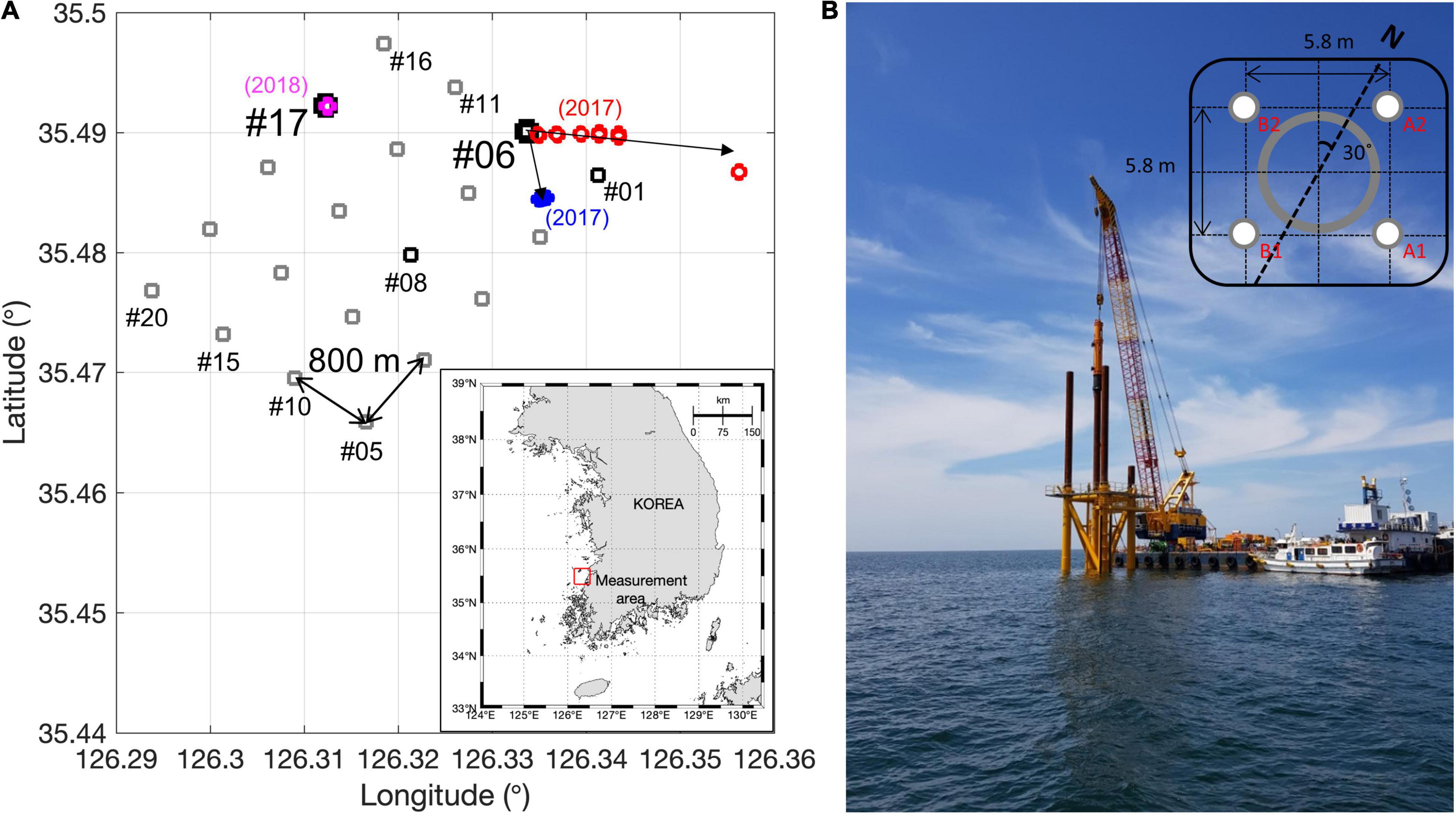
Figure 1. (A) Location of “Southwest offshore wind farm” located on the southwest coast of Korea and layout of twenty offshore wind turbines. Black squares indicate wind turbines that are either completed or under construction and gray squares indicate the expected locations for wind turbine installation. Circles represent measurement points. (B) Photograph of wind turbine construction. (Inset) Schematic diagram of wind turbine 6 consisting of four piles (A1, A2, B1, and B2).

Measurements were first made as a function of strike number for pile B2 at a point ∼640 m away from the pile after anchoring the vessel (blue circles in Figure 1A). Next, impact pile driving noise as a function of range was measured at distances of 112, 288, 520, 695, 884, and 2,077 m, while drifting the vessel in an easterly direction (red circles in Figure 1A). Acoustic data at distances of 112, 288, and 520 m were measured during piling work for pile A1. Pile A2 corresponded to distances of 695 and 884, and pile B1 corresponded to 2,077 m.

The second additional measurements were performed in April 2018 to acquire the time-separated multipath arrivals of impact piling driving noise. The measurements were made on a turbine 17 using the same 3-channel hydrophone array used in 2017 and the distance from the pile ranged from 15 to 24 m (magenta circles in Figure 1A). All acoustic measurements were conducted in accordance with an international standard and guide (Robinson et al., 2014; International Organization for Standardization [ISO], 2017b) with the vessel engine off.

The maximum stroke strength of the piston and the potential energy were 2,000 mm and 284 kN-m, respectively, and the impact energy of 142 kN-m was constant during the installation of four piles except for a few strokes at the beginning of each pile installation. The length of the pile was 80.7 m, with a diameter 0.9 m, and the pile material was a structural steel (S355). According to several manufacturers, the density ρ_p of the structure steel S355 is reported in the range of 7,700 and 7,850 kg/m³, but there are few reports on the sound speed. The density and the compressional sound speed c_p of 7,700 kg/m³ and 5,950 m/s, used by Zampolli et al. (2013) for their model prediction were used in this paper. Because the sound speed in the pile is much higher than that of water, it was expected that the Mach wave was transmitted down through the pile and radiated into the water medium at an angle of ∼14.9°C.

Pile driving produces an impulse-shaped waveform, and therefore, it can be characterized using sound exposure level L_E and peak sound pressure level L_P, which measure the total energy for the duration of exposure and the maximum zero-to-peak pressure of the exposure signal, respectively. These are given by:

$L_E=10\mathrm{l}{\text{og}}_{10}\left(\frac{E_p}{E_{p,0}}\right),\mathrm{where}{E}_p={\int }_{t_1}^{t_2}{p}^2\left(t\right)\mathit{dt}(3)$

$L_p=20\mathrm{l}{\text{og}}_{10}\left(\frac{p_{pk}}{p_0}\right),(4)$

where p(t) and p_pk are the measured pressure signal and its peak absolute value, respectively. p₀ is a reference value of sound pressure (equal to 1μPa) and E_p,0 = 1μPa²s is the reference value of the time-integrated squared sound pressure. t₁ and t₂ are the start and end points of time window, respectively, for consideration of the exposure duration (International Organization for Standardization [ISO], 2017a).

The spectrum of pile driving noise can be expressed in energy spectral density (ESD), which is commonly used to describe impulsive-type signals, and the ambient noise is expressed in power spectral density (PSD):

$\int P{\left(t\right)}^2\mathit{d}t={\int }_0^{f_{max}}E\left(f\right)\mathit{d}f(5)$

$\frac{1}{T}\int P{\left(t\right)}^2\mathit{d}t={\int }_0^{f_{max}}P\left(f\right)\mathit{d}f(6)$

where E(f) is the ESD in units of μPa²sec/Hz and P(f) is PSD in μPa²/Hz (Carey, 2006). Here, a time duration of 1 s was used in the ESD analysis, making the ESD of impact pile driving noise directly comparable to the PSD of ambient noise.

Results

Acoustic Properties of Pile Driving Noise

The waveform of pile driving noise consisted of several Mach waves propagating downward and upward along the pile, producing an axisymmetric and cone-shaped acoustic field called a Mach cone (Reinhall and Dahl, 2011). The first phase is a down-going cone that arrives first with the highest amplitude, the second phase is a Mach cone traveling upward and originating from a reflection of the first down-going Mach wave at the end of the pile, and the third phase is another reflection from the top of the pile, reproducing the downward wave. Additional subsequent phases are also generated, but they are negligible owing to the superposition of reflection loss at the pile-bottom interface (Reinhall and Dahl, 2011). The first phase separated in time from the subsequent phases can generally be measured in the range of less than H/tan(θ_w), where H is the water depth (Reinhall and Dahl, 2011). Because the measurements of impact pile driving noise at the distance satisfying this condition were not made during the construction of turbine 6, the measurements of the time-resolved the first-phase waveform were conducted in April 2018. In our case, which corresponds to a water depth of ∼12 m, it is expected that it can be measured at distances of less than 45 m. The time lag between first and third phases, which can be estimated by dividing twice the pile length by the compressional sound speed, was estimated to be 25.2 ms for the pile length of the turbine 17 (75.12 m), assuming a reported pile sound speed of 5,950 m/s (Zampolli et al., 2013). However, the time lag between the first and second phases depends on the penetration depth of the pile into the sediment (Reinhall and Dahl, 2011). In our case, the time lag between the first and second phases are predicted to increase from ∼2.6 to 15.8 ms as the wetted pile length increases. Wetted pile length means the length of the pile immersed in water and sediment. Figure 2A shows an ensemble average of 55 waveforms acquired by a hydrophone placed 4 m above the water-sediment interface in April 2018. Three thick black lines are the estimated first, second and third phases in this order. Red and magenta dashed lines are the first-phase waveform, weighted by –0.7 and 0.3, with time delays of 12.8 and 25.5 ms, respectively, for comparison with the second and third phases. The normalized spectrums of the first phases of 55 waveforms and their average were shown in Figure 2B, which was obtained from the square root of the average of magnitude-squared spectra of the first phase smoothed with a Tukey window. An angle-of-arrival analysis was performed to estimate the arrival angle using the first phase waveforms received from three vertically placed hydrophones. The arrival angle was estimated to be approximately ∼14.5°C, which is very consistent with the value predicted by Eq. (1) using the sound speed of the pile (5,950 m/s) used by Zampolli et al. (2013).

FIGURE 2

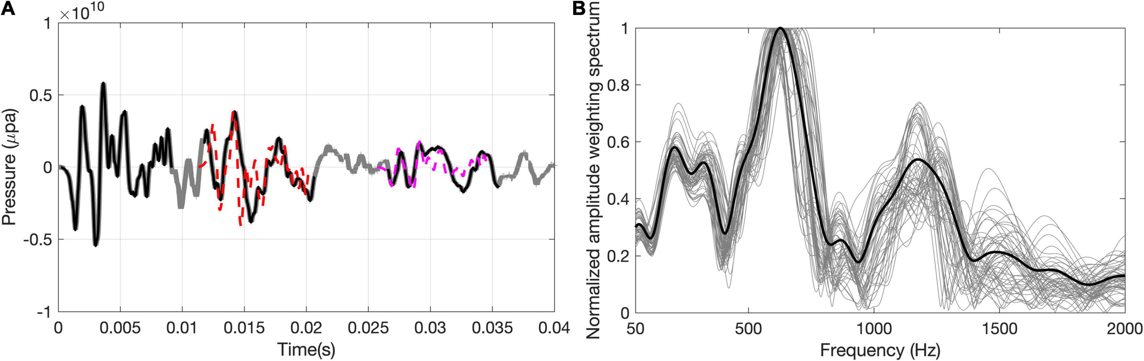
Figure 2. (A) Ensemble average of 55 waveforms acquired by a hydrophone placed 4 m above the water-sediment interface at distances of 15–24 m from the turbine 17. (B) Normalized amplitude-weighting spectrums estimated from the 55 first phase waveforms and their average spectrum (thick black line), which was used in the broadband PE simulation.

Figures 3A,B show the snapshots of the first three pile driving pulses and their corresponding spectrograms, respectively, which were acquired at a bottom receiver positioned approximately 3 m above the seafloor and 639 m from the source in 2017. Impact pile driving noises were received approximately every 1.2 s. The waveform was impulse-like and 90% the energy was included within 100 ms, although the reverberant tail lasted until the next snapshot was received. The beginning of each signal was broadband but higher-frequency components decayed quickly, leaving only energy at frequencies of less than ∼2,000 Hz after ∼100 ms (Figure 3B).

FIGURE 3

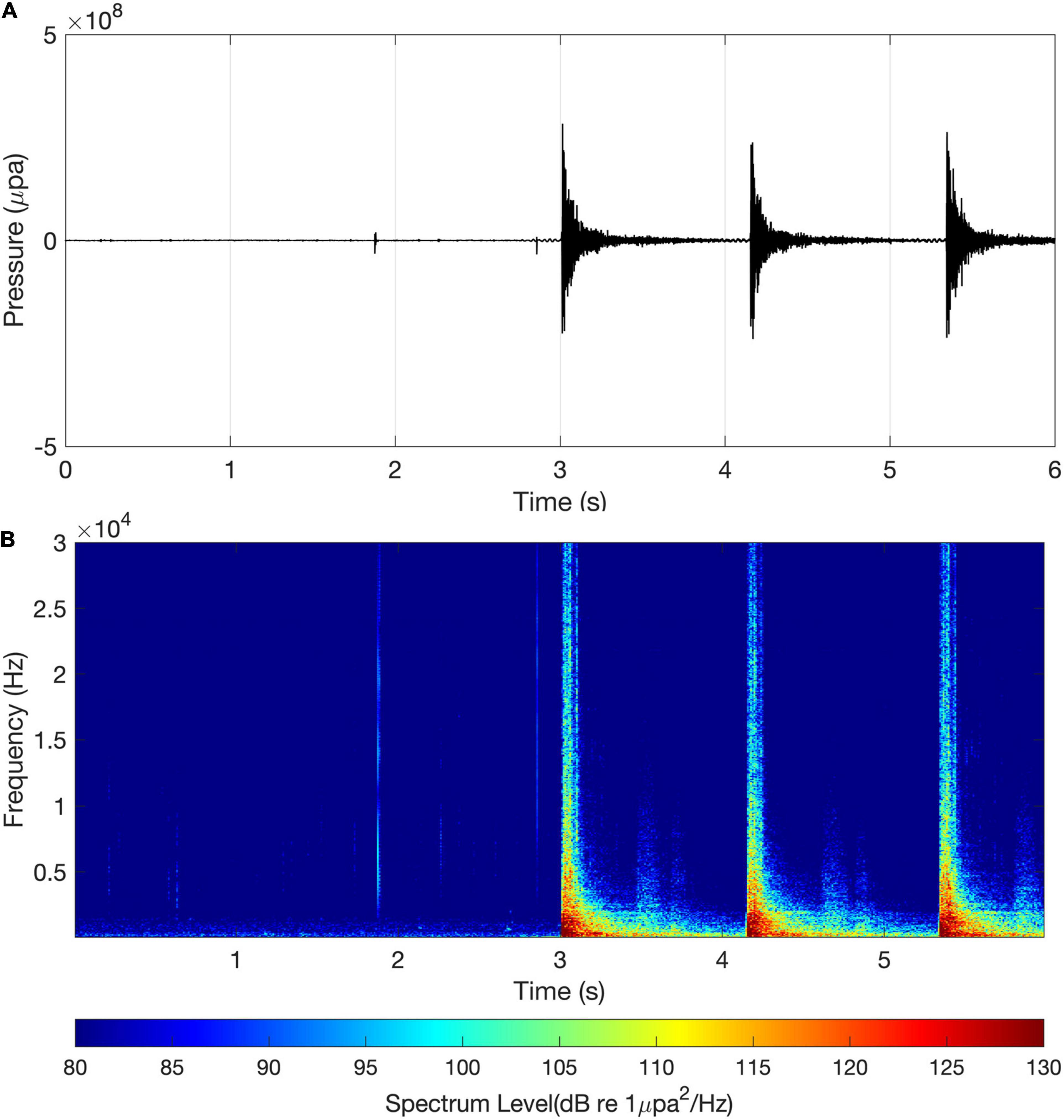
Figure 3. (A) Time series and (B) the spectrogram of impact pile driving noise measured ∼639 m from the pile and a depth of 3 m above the seafloor.

Figure 4 shows the ESD averaged for pile driving noise received by three hydrophones for 200 pile driving pulses for pile B2 at a point approximately 640 m from the pile. For the ESD estimates, a time series 1 s long for each impact pile driving event was extracted such that the main arrival was approximately 0.1 s within the time window. The data were then demeaned and tapered using a Tukey window with a taper parameter of 0.2. In the ESD, several prominent peaks with a mean frequency interval of approximately 38 Hz were observed between 80 and 500 Hz, which is the inverse of the time lag between the first and third phases. Because the estimated time lag was 27.1 ms, its inverse was approximately 37 Hz, which was consistent with the frequency interval of peaks of ESD of impact pile driving noise. The background ambient noise was also measured before and after the pile driving operation and their PSDs were analyzed using the same Tukey window used for the ESD analysis, which was directly compared to the ESD of impact pile driving noise.

FIGURE 4

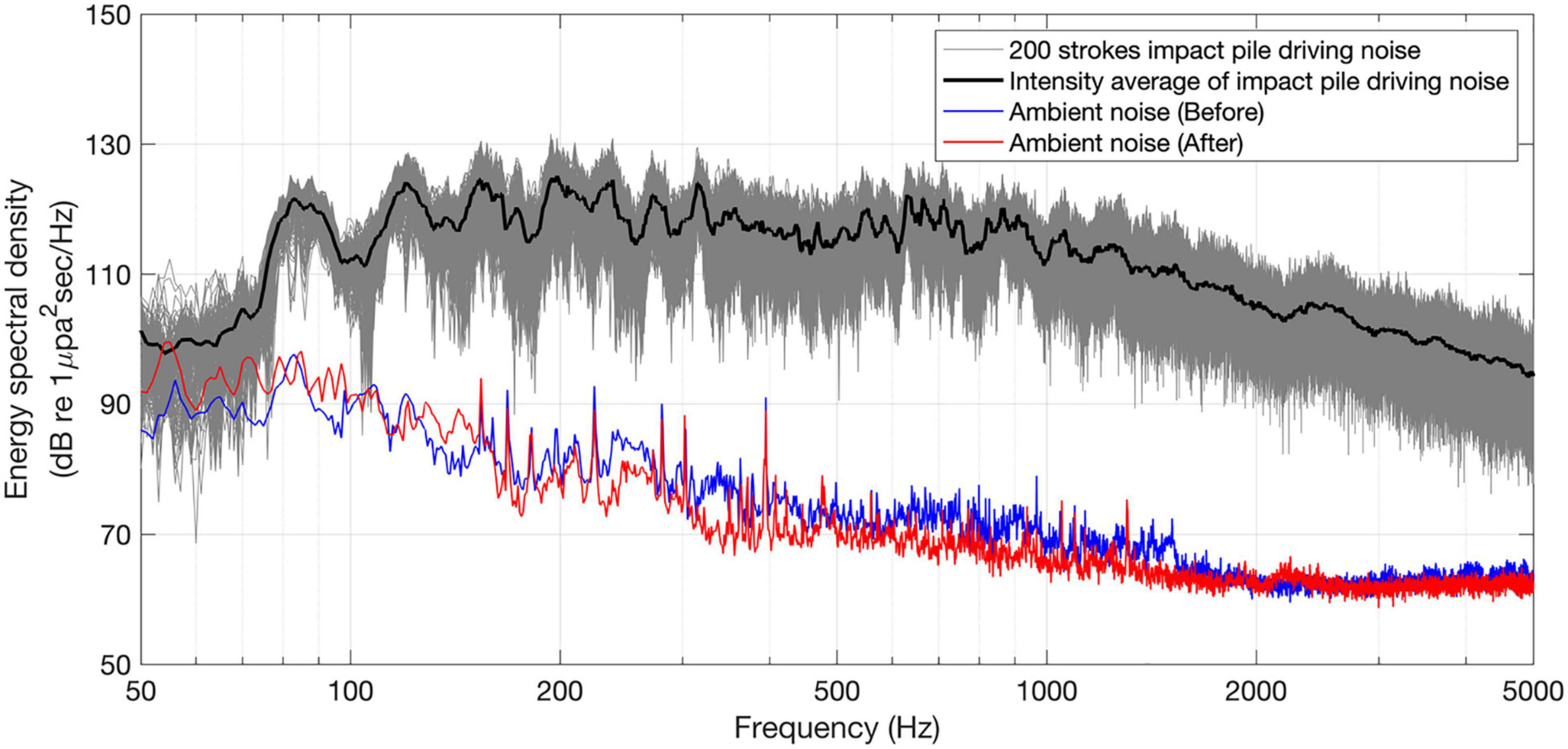
Figure 4. Comparison of the spectrum levels between impact pile driving noise for pile B2 and ambient noise. The thick black line represents the depth-averaged ESD of pile driving noise averaged for 200 snapshots. The thin blue and red lines display the PSD of ambient noise measured before and after the pile driving operations.

Variation of Pile Driving Noise With Hammer Blows

Hammer blows were repeated until the pile was driven to the required depth. At early stages of the blow process, called a soft-start period, the pile was driven with low stroke energy to induce the escape of marine animals in the vicinity, and then the hammer energy was gradually increased to reach half its maximum stroke strength (Robinson et al., 2007). In the case of pile B2, the hammer blows were repeated 622 times for 14 min, including the soft-start period corresponding to the initial 10 hammer blows. Figures 5A,B, respectively, depicts the measured sound exposure levels and peak sound pressure levels as a function of the number of hammer blows for 200 strokes. Only data prior to the 211th hammer blow were used because the vessel from which the receiver system was deployed drifted in ocean currents after the 210th stroke. Data for the initial 10 blows corresponding to the soft-start period were also excluded. The value of the sound exposure level at 3, 5, and 7 m above the seafloor were nearly constant, with the values of 148.5 ± 2.1 dB, 148.2 ± 2.1 dB, and 149.1 ± 2.1 dB, respectively. In the case of peak sound pressure, the difference in depth was slightly larger than that of the sound exposure level, but the values were stable with respect to the hammer blow number, showing the values of 170.3 ± 2.2 dB, 169.7 ± 2.1 dB and 173.7 ± 2.1 dB at 3, 5, and 7 m above the seafloor, respectively. Statistical fluctuations in the level for three depths were in a range of ± 0.5 and ± 0.6 dB based on 200 strokes, which were added in quadrature to the uncertainty of receiving voltage sensitivity of hydrophone, ± 2.0 dB to estimate the total measurement error (International Organization for Standardization [ISO], 2017b). Now, the sound exposure levels and the peak sound pressure levels for three depths were depth averaged for comparison with the predictions by DCSM, which were 148.6 ± 2.1 dB and 171.6 ± 2.8 dB, respectively.

FIGURE 5

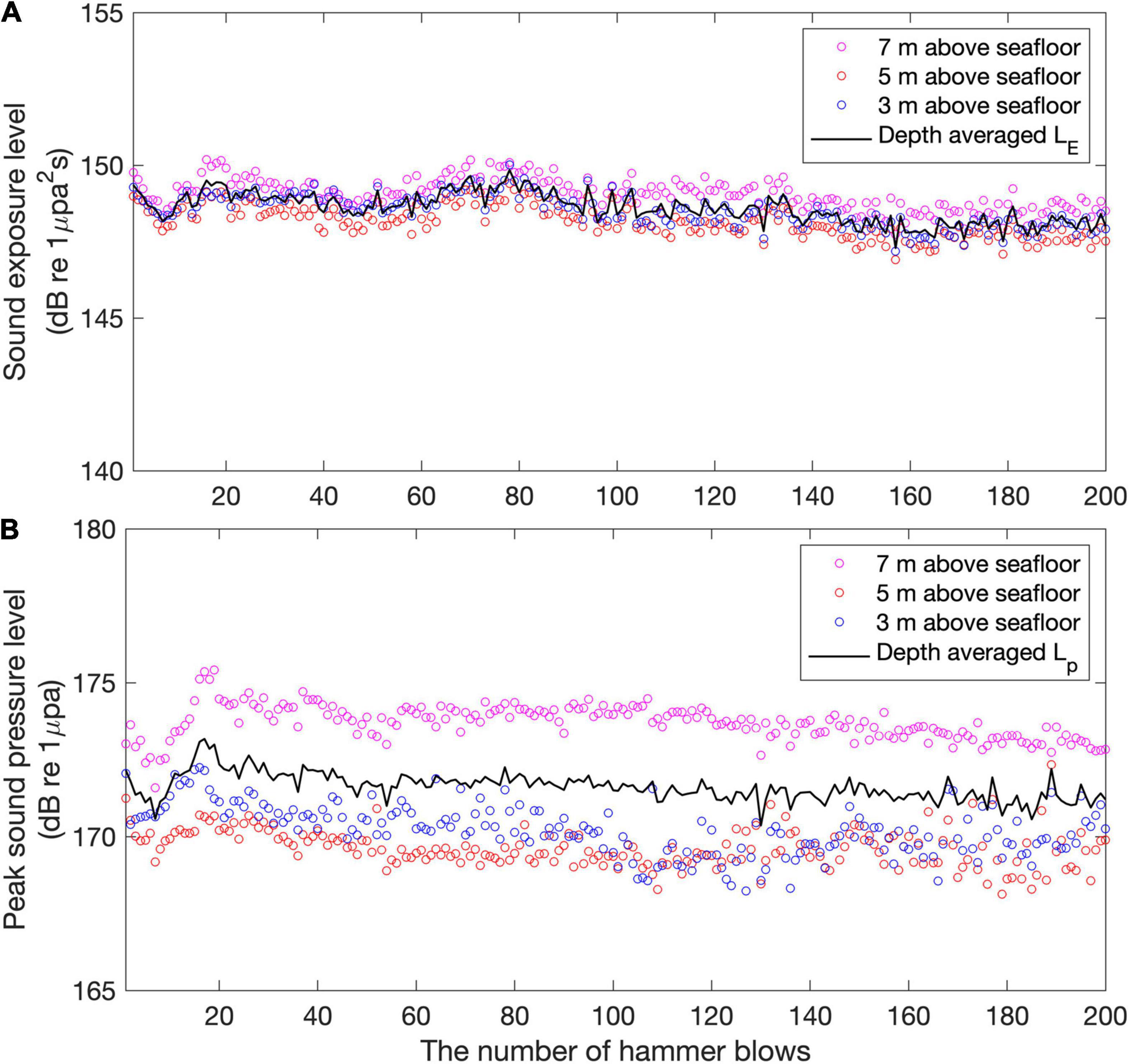
Figure 5. (A) Measured sound exposure levels and (B) peak sound pressure levels as a function of the number of hammer blows. The blue, red, and magenta circles for both cases represent the values measured at the depths of 3, 5, and 7 m above the seafloor, respectively. Thick black lines indicate the depth-averaged noise levels.

Variation of Pile Driving Noise With Distance

To investigate the propagation properties of the impact pile driving noise as a function of distance, measurements were made at 112, 288, 520, 695, 884, and 2,077 m from turbine 6. Figure 6 shows the measured sound exposure levels and peak sound pressure levels as a function of distance and their comparisons with a regression curve based on a simple transmission-loss model. The pressure levels at 112, 288, and 520 m were estimated using data collected during the piling work for A1. Those at 695 and 884 m were obtained from the data from pile A2, and the levels at 2,077 m were obtained from pile B1 data. Blue, red, and magenta circles represent the noise levels at depths of 3, 5, and 7 m above the seafloor, respectively. Black circles represent the depth-averaged noise levels, for which mean values and their estimated uncertainties are listed in Table 1. Distance errors caused by ship drifting were negligible, less than ∼10 m. Note that the difference according to the penetration depth of the pile into the sediment was not included in the uncertainty of our data. As mentioned in section “Comparison With Parabolic Equation-Based Propagation Model,” a trial has been made to measure the impact pile driving noise from the beginning to the end of the pile driving process on a single pile at a point ∼640 m away from the pile. But because the vessel drifted, only data corresponding to the first 200 stokes could be accepted as data obtained from a single point. Assuming that the penetration depth of the pile increases at a constant depth interval for each stoke, the penetration depth in the sediment layer corresponding to the first 200 stokes ranges from 0 to 20 m (for reference, the final target penetration depth of the pile immersed in the water and sediment was 60 m). The difference in the received noise level due to this difference in penetration depth was estimated to be less than ± 0.6 dB (see Figure 5). Dahl and Dall’Osto (2017) estimated that the difference due to the penetration depth would be on the order of 3 dB based on observations of impact pile driving at range 12 m during which penetration depth was increasing; this change was also reflected in their modeling.

FIGURE 6

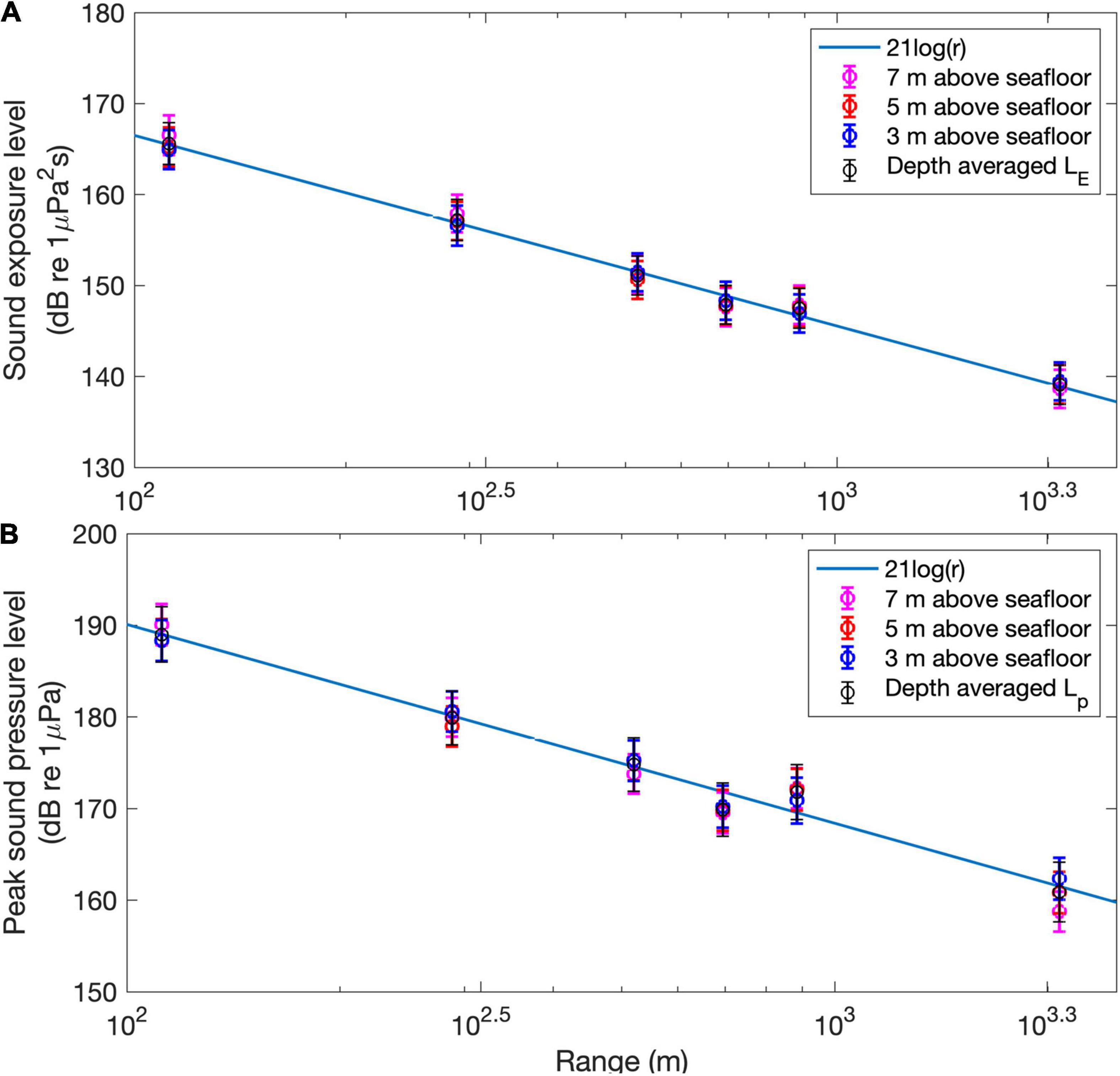
Figure 6. (A) The sound exposure levels and (B) peak pressure levels estimated as a function of distance (blue, red, and magenta are those measured at 3, 5, and 7 m above the seafloor, respectively) and their comparisons with the regression curves corresponding to 21log⁡r+ C.

TABLE 1

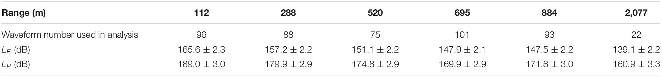
Table 1. Sound exposure levels and peak pressure levels estimated for impact pile driving noise as a function of distance.

The simple transmission-loss model is defined by Nlog⁡r + C, where N is a spreading constant, and C is an offset constant. In both cases, the regressive curve that best fitted the data was 21log⁡r, with different arbitrary decibel offsets, which was slightly higher than the transmission loss for spherical spreading alone (= 20log⁡r). A strong acoustic interaction with the seafloor due to a downward radiation of impact pile driving noise appeared to result in a relatively rapid energy loss with increasing distance.

Comparison With Model Predictions

Comparison With Damped Cylindrical Spreading Model

The DCSM is a simple prediction model defined by Equation (2) based on cylindrical spreading. Additional loss other than cylindrical spreading loss is considered with a frequency-independent decay factor α (in decibels per meter), which is defined by Lippert et al. (2018):

$\mathrm{\alpha }=\frac{-10{\text{log}}_{10}({\left|R\right|}^2)}{2Hcotan({\mathrm{\theta }}_w)},(7)$

where R is a Rayleigh reflection coefficient at the water-sediment interface (Frisk, 1994). The acoustic parameters used to estimate the decay factor are listed in Table 2. The sound speed of the pile was assumed to vary between 5,950 and 6,140 m/s. The lower bound was a value used in a previous study (Zampolli et al., 2013). The upper bound was estimated using the pile driving noise measured at a point 640 m from the pile for pile B2, which was estimated by dividing the twice the pile length by the time lag between first and third phases (the inverse of the frequency interval of the spectrum peaks in ESD in Figure 4). Because the water depth decreased slightly from 12 m at the piling position to 10 m at 2,100 m, water depths between 10 and 12 m were considered in Equation (7). The ranges of sound speed, density, and attenuation in sediment were determined by a mid-frequency geoacoustic model (Bachman, 1985). Geoacoustic parameters were used to calculate the bottom reflection coefficient in Equation (7). Figure 7 compares the depth-averaged sound exposure levels as a function of distance and the DCSM prediction curve obtained using 288 m as the reference distance. The model input parameters were randomly selected in ranges suggested in Table 2 using a Monte Carlo simulation. A total of 10⁸ random runs were made. The thick dashed line in Figure 7 represents the model curve predicted using the best-fit decay factor, which was 6.2 dB/km. Two thin, gray, dashed lines show the upper and lower bounds of model predictions, which correspond to decay factors of 3.5 dB/km and 12 dB/km, respectively. The effect of the reference distance on DCSM accuracy was investigated by Lippert et al. (2018), who concluded that the DCSM was more or less independent of the choice of reference distance. The DCSM predictions that best fitted the measured depth-averaged sound exposure levels were performed using six distances each as the reference distance. The model predictions for the five distances except for the reference distance of 112 m were similar, showing best-fit decay factors between 5.0 and 6.2 dB/km. However, the best-fit decay factor predicted using 112 m as the reference distance was 8.8 dB/km, which was slightly higher than the other cases.

TABLE 2

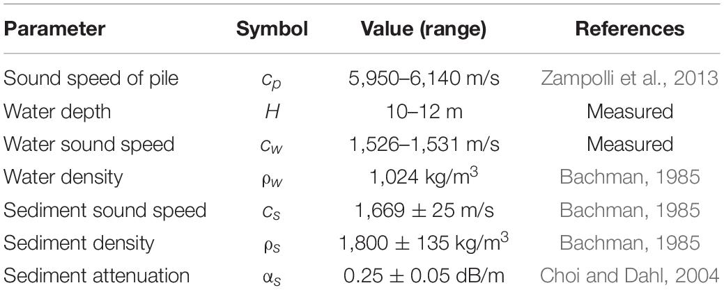
Table 2. Input parameters used for the DCSM predictions.

FIGURE 7

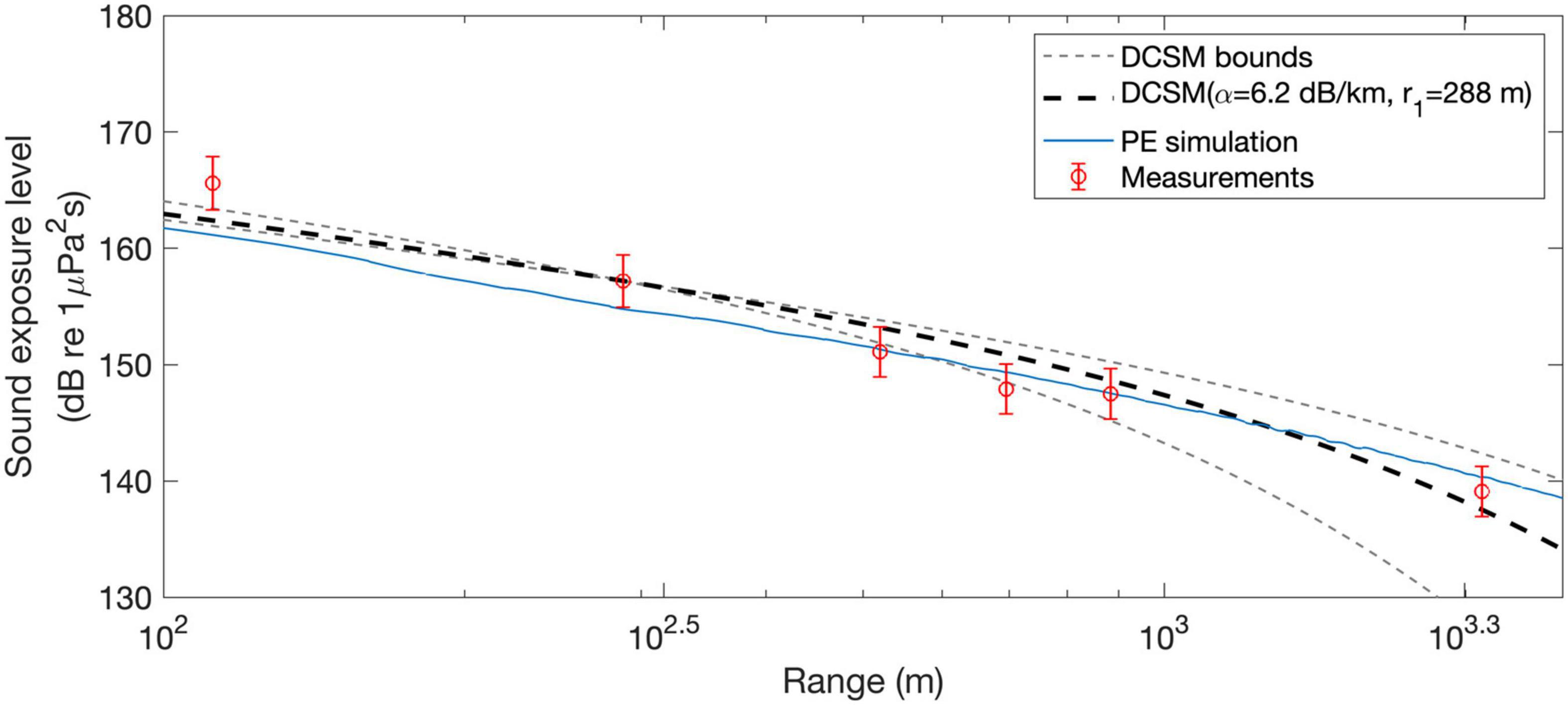
Figure 7. Measured depth-averaged sound exposure levels (red circles) as a function of distance and a comparison with model predictions. Thick dashed line is the best-fitted DCSM predictions obtained using a reference range of 288 m. Two thin gray dashed lines represent upper and lower bounds of the DCSM predictions obtained using decay factors estimated from the combination of input parameters listed in Table 2. The blue solid line represents the depth-averaged sound exposure level curve predicted by the broadband PE simulation.

Comparison With Parabolic Equation-Based Propagation Model

This section compares the measured sound exposure levels with those predicted by the broadband PE simulation using the RAM. The frequency band between 50 Hz and 2 kHz was considered, and the environmental conditions at the site, such as sound speed in water, bathymetry, and geoacoustic parameters in sediment, were used as model input. The PE simulation of the impact pile driving noise was based on the method presented by Reinhall and Dahl (2011). Because Mach wave propagates along the pile, the pile was assumed to be a vertical-line array source with directivity from Equation (1). It was assumed that 120 virtual point sources were distributed along the pile from 0.5 to 60 m at intervals of 0.5 m because the final penetration length of the pile immersed in the water and sediment was 60 m.

Figure 8 shows the geometry and bathymetry used in the PE simulation. Because the surficial sediment at the site consisted of sand with a mean grain size of 4.0ϕ, frequency-dependent dispersion corrections for the sediment sound speed and sediment attenuation were made based on Biot theory (Williams et al., 2002; Zhou et al., 2009), and the sediment sound speed from 1,566 to 1,725 m/s and sediment attenuation from 0.001 to 1.202 dB/m were used within the frequency range of 50 Hz to 2 kHz. The sediment density was assumed to be 1,800 kg/m³, based on the empirical formula (Bachman, 1985).

FIGURE 8

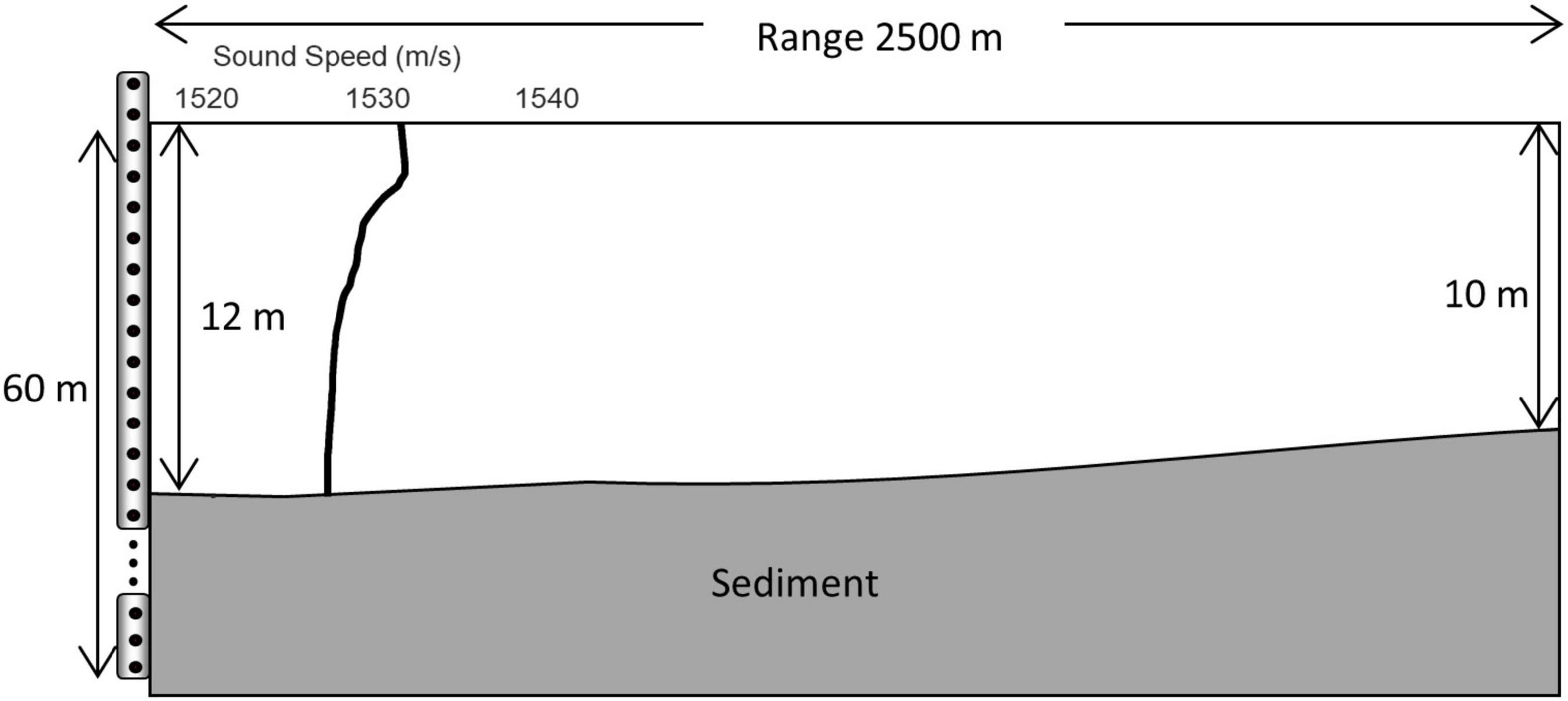
Figure 8. Bathymetry of the site and the geometry showing virtual acoustic point sources. The thick solid line in water column represents the sound-speed profile with depth.

The acoustic fields emitted from the pile can be expressed as a function of frequency at receiver position (r,z):

$p_i(r,z,f)=\sum _{m=1}^M{G}_{i,m}(r,z,f)A\left(f\right)e^{-i\mathrm{\omega }{\mathrm{\tau }}_{i,m}},(8)$

where G_i,m(r,z,f) is Green’s function, which is a point-source response predicted by the RAM for the m-th point source at the i-th phase. ω is the angular frequency, and τ_i,m is the time delay of m-th point source, which is equal to the time it takes for the signal generated at the top of the pile source by hammering to reach the m-th point source. For the first phase, this corresponds to a depth of the m-th point source divided by c_p. In this study, only the first three phases were considered because the energies of the subsequent phases were negligible due to the superposition of reflection loss at the pile-bottom interface (Reinhall and Dahl, 2011). A(f) is an amplitude-weighting spectrum corresponding to the normalized source spectrum of pile driving noise (see Figure 2B).

The total acoustic field radiated from the pile can be predicted by the coherent summation of three phases:

$P(r,z,f)=p_1(r,z,f)+{\mathrm{\kappa }}_2{p}_2(r,z,f)+{\mathrm{\kappa }}_3{p}_3(r,z,f)(9)$

where κ_i is the amplitude scaling factor of each phase, which is related to the reflection coefficient at each end of the pile and is determined by the amplitude ratio between the first phase and other phases. In our case, κ₂ and κ₃ were estimated to be approximately –0.7 and 0.3, respectively.

The sound exposure level for the broadband signal can be estimated using Parseval’s theorem (Ainslie, 2010; Dahl and Dall’Osto, 2017) as follows:

$L_E(r,z)=-10{\log }_{10}\text{[}\frac{1}{B}\int P(r,z,f)P^{*}(r,z,f)df]+K,(10)$

where B is the frequency bandwidth (50 Hz to 2 kHz in the simulation). The asterisk means a complex conjugate and K is an offset constant.

Figure 9A shows the PE-simulated acoustic field produced by the impact pile driving as a function of depth and distance, in which ρ_p and c_p used in the simulation were 7,700 kg/m³ and 5,950 m/s, respectively. The offset constant K was 185.9 dB, which was derived from a least-squares fit between the simulated acoustic field and the sound exposure levels measured at 18 points marked in Figure 9A. The strong interference patterns by the Mach cones propagating up and down are seen in the simulated acoustic field.

FIGURE 9

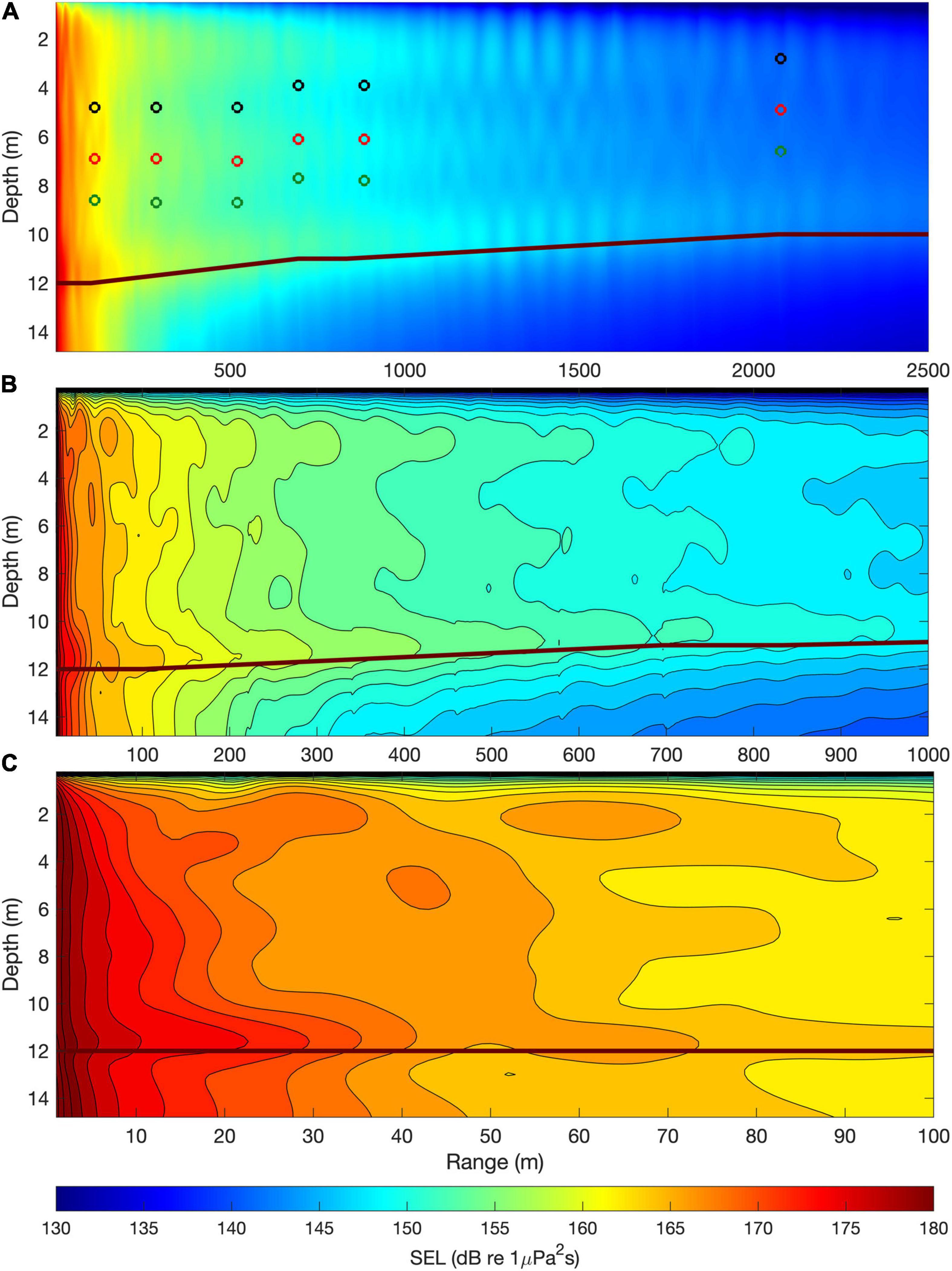
Figure 9. (A) PE-simulation of acoustic field produced by the impact pile driving. Hydrophone positions were marked with circles (green, red, and black positions are 3, 5, and 7 m above the seabed). The brown line represents the water-sediment interface. Water depths gradually decreased as the distance from the pile increased. (B) Expanded view of the simulated acoustic field with contours up to the distance of 1,000 m. (C) Further expanded view up to distance of 100 m.

The PE outputs were depth-averaged and compared with the measurements and the DCSM prediction, as shown in Figure 7. The blue solid line represents the depth-averaged sound exposure level curve predicted by the broadband PE simulation, which is also in agreement with the measured sound exposure levels of the impact pile driving noise. The root mean square errors between the measurements and model predictions from DCSM and PE simulation were 2.1, 2.2 dB, respectively. The sound exposure source levels at 1 m from the pile predicted by the DCSM and the PE simulations were 184 and 183 dB re 1μPa²s, respectively. Although the specifications of the hammer and pile were not the same, the predicted source level was comparable to that reported previously (Leunissen and Dawson, 2018).

Summary and Discussion

Impact pile driving noise was measured as a function of distance on the southwest coast of Korea. Sound exposure levels were measured at three depths corresponding to 3, 5, and 7 m above the seafloor at six points at distances of 100–2,100 m and compared with predictions from the DCSM and broadband PE simulation. The DCSM is a simple model based on cylindrical spreading with a decay factor related to the environmental acoustic properties of the site, producing depth-averaged sound exposure levels as a function of distance. The broadband PE simulation predicted the sound exposure levels as a function of depth and distance, assuming that the pile was a vertical-line array source with a beam pattern of axisymmetric Mach cone. The broadband PE simulation results as a function of distance, obtained using the geoacoustic properties of surficial sediments, were in close agreement with the measurements. However, it is necessary to use the geoacoustic information including sub-bottom layers as model inputs to obtain more accurate model predictions because the low-frequency sound propagation, which is a predominant component of pile driving noise, can be greatly influenced by geoacoustic properties of sub-sediment layers. The sound exposure levels averaged for three depths were in close agreement with both model predictions.

Several studies reported that the noise level of pile driving noise near the seafloor was generally higher than at the sea surface (Reinhall and Dahl, 2011; Tsouvalas, 2020). However, in our case, which was measured at approximately 640 m from the pile in 2017, the sound exposure level and the peak pressure level were the lowest at 5 m above the seafloor, and rather higher at 3 and 7 m above the seafloor, as shown in Figures 5A,B. Figures 9B,C show the simulated acoustic field as a function of depth and distance up to a distance of 1,000 m, and its expanded view up to a distance of 100 m, respectively. Overall, in our case, it is also simulated to have higher noise levels near the seafloor. However, there is a variation in the noise level with depth due to strong acoustic interference of down and upward radiations. That is, it is simulated that there are layers with somewhat higher noise levels even in the surface layer at a depth of about 2–3 m and in the middle layer at a depth of about 6–7 m. The strong acoustic interaction with the seafloor of the Mach-cone wave sequence radiating upwards and downwards appears to cause relatively rapid energy loss with increasing distance, and thus the depth-averaged noise level tended to decrease with increasing distance, following 21log⁡r in our case.

The amplitude scaling factor (κ_i) in broadband PE simulation was different from the previous study. Reinhall and Dahl (2011) estimated the value of κ₂ for the second phase to be approximately − 0.38. They assumed that the reflection at the top of the pile was subject to the strain relief boundary, and therefore the third phase was approximately an inverse second phase without additional amplitude reduction (that is, κ₃≈ 0.38). This differs from our results in that the amplitude of the third phase was somewhat reduced compared with that of the second phase. The reason for this difference was not evident. However, a diesel hammer was used in Reinhall and Dahl (2011), whereas a hydraulic hammer was used in our case. The primary parts of pile driving system at the top of the pile are the helmet and hammer. Typically, the helmet consists of several components, such as a cap, hammer cushion, pile cushion, and striker plate (Hannigan et al., 2006). The hammer cushion protects the ram against metal fatigue due to the repetitive shock loads, and the pile cushion is used to protect the top of the pile (Lucieer, 2000). Some of components may differ or not exist depending on the hammer type (Hannigan et al., 2006). The acoustic characteristics of these components may affect the amplitude of the third phase. The hammer used in the construction included a plastic hammer cushion, but there was no pile cushion. However, we do not know the exact structure of the hammer in more detail.

Based on the model predictions, the sound exposure source levels were predicted to be approximately 183–184 dB re 1μPa²s. The spatial distribution of the impact pile driving noise can be predicted using the broadband PE model. Figure 10A is a contour map of the depth-averaged sound exposure level predicted for turbine 6 using a sound exposure source level of 183 dB re 1μPa²s, and Figure 10B depicts the bathymetry of the site used in the PE simulation, which was extracted from Global Multi-Resolution Topography data (Ryan et al., 2009). The sound-speed profile in Figure 8 was used for predictions on the assumption that the sound-speed profile is spatially identical. The depth-averaged sound exposure level as a function of distance was predicted for 36 azimuthal angles at 10° intervals for the turbine-6 position and then interpolated to obtain the contour map. Combining the spatial distribution simulation result of the impact pile driving noise with the noise-induced damage threshold of local marine life, it may be possible to assess the environmental impact of the wind power plant construction on marine ecosystems. Yellow croaker (Larimichthys polyactis), for example, is one of the most abundant fish in the region where the Southwest offshore wind farm is located (National Institutes of Fisheries Sciences [NIFS], 2017). Popper (2008) reported that the Atlantic croaker belonging to the same croaker family (Sciaenidae), although not the same species as yellow croaker, detects sounds from 0.1 to 1.0 kHz and is most sensitive at 0.3 kHz. In addition, hearing loss in marine mammals exposed to loud noise has been investigated in some previous studies. Nehls et al. (2007) summarized the recommended values for Temporary Threshold Shift (TTS) and Permanent Threshold Shift (PTS) in the results of Ketten and Finneran (2004). In other words, for cetaceans, TTS and PTS were recommended at 183 and 215 dB re 1μPa²s in sound exposure level, respectively, and the TTS for Pinnipeds was recommended at 163 dB re 1μPa²s in sound exposure level. Applying the TTS for Pinnipeds to the spatial distribution simulation results, the spatial extent that can affect the TTS for Pinnipeds can be estimated with a radius of about 0.11–0.14 km from the pile. However, the physical damage to marine life due to anthropogenic noise should be carefully discussed through multidisciplinary assessments.

FIGURE 10

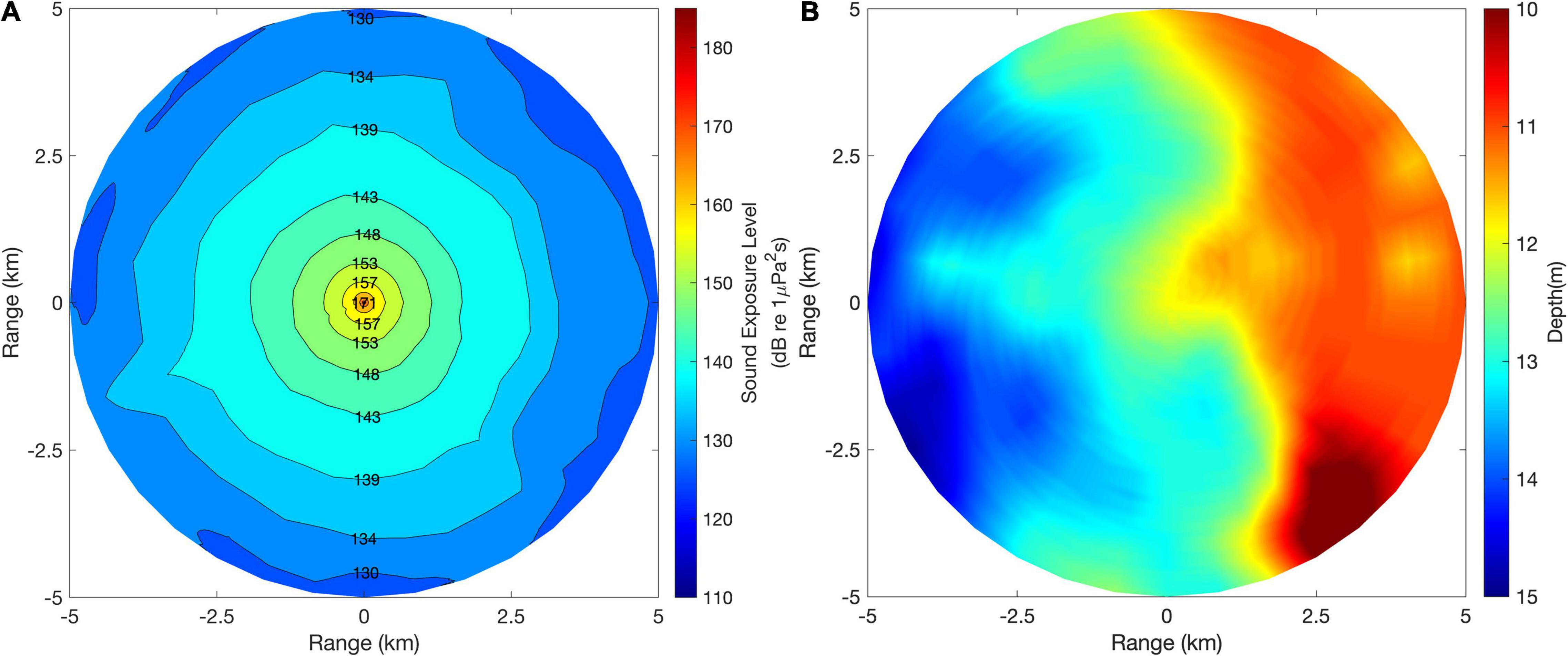
Figure 10. (A) A contour map of depth-averaged sound exposure level of impact pile driving noise predicted by the broadband PE model using a sound exposure source level of 183 dB re 1μPa²s, and (B) the topography of the target area (5 km ×5 km) extracted from the Global Multi-Resolution Topography data.

Finally, the relation between the peak sound pressure level and the sound exposure level was investigated. Previous studies (Galindo-Romero et al., 2015; Lippert et al., 2015) used a linear regression curve equation, which is given by L_P=AL_E + B, where A and B are empirical constants. Figure 11 depicts the relationship between peak sound pressure levels and sound exposure levels of the impact pile driving noise measured at three depths and six distances, and the best-fitted regression curve line obtained using constants for A and B of 1.0 and 20, respectively. The constant values are somewhat different from those presented in Lippert et al. (2015). However, this difference was reasonable because both constants are related to environmental properties and pile characteristics. That is, the constant A is related to the change of peak value with energy change and thus is related to the properties of the waveguide. The constant B is a variable that determines the initial relationship between the peak sound pressure level and the sound exposure level, and is thus related to source attributes such as pile and hammer characteristics (Lippert et al., 2015). Because the broadband PE simulation predicted the sound exposure source level to be ∼183 dB re 1μPa²s, the source peak sound pressure level at 1 m was estimated to be 203 dB re 1μPa using the best-fitted regression curve.

FIGURE 11

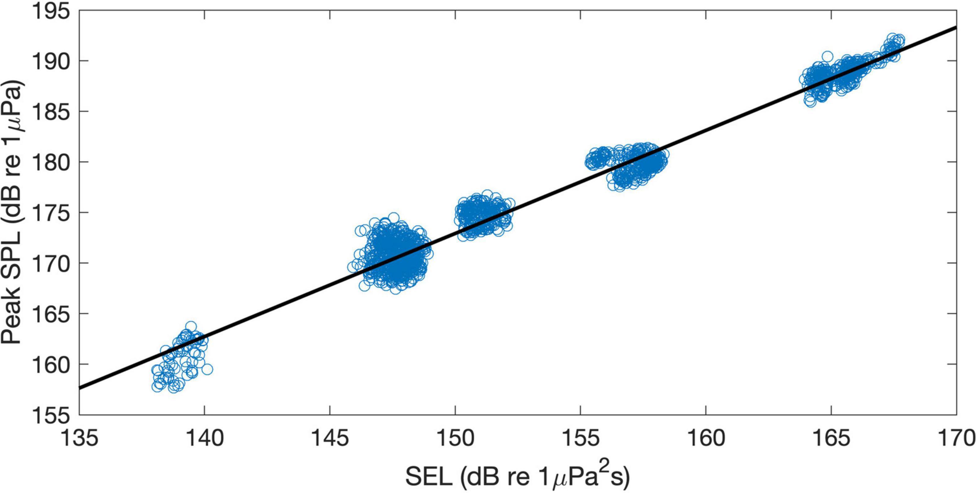
Figure 11. The relation between peak sound pressure level and sound exposure level estimated from the data recorded at the six distances and three depths (blue circles). The black line represents the best-fitted regression curve, which is equal to L_P=L_E + 20.

Over the last century, as human activities in the ocean have increased, so has underwater ambient noise (Dahl et al., 2007; Slabbekoorn et al., 2010; Chapman and Price, 2011; Frisk, 2012), in part due to offshore wind power plants construction activities. It is therefore important to assess the noise impact, including the measurements of pile driving noise levels, and investigate their propagation properties as a function of distance in an underwater waveguide. In this paper, impact pile driving noise was measured and analyzed in one specific area off the Korea peninsula, but the effects of noise generated by various piles and hammers on the marine environment should be continuously investigated in various area.

Data Availability Statement

The original contributions presented in the study are included in the article/supplementary material, further inquiries can be directed to the corresponding author/s.

Author Contributions

D-GH carried out acoustic data analysis and propagation modeling. JWC contributed to the supervision and validation of the measurement and prediction results. Both authors contributed to the writing of the original draft.

Funding

This research was supported by Korea Institute of Energy Technology Evaluation and Planning (KETEP) grant funded by the Korea Government (MOTIE) (20203030020080, Environmental Impact Analysis on the Offshore Wind Farm and Database System Development) (JWC) and the “Ecosystem structure and function of marine protected area (MPA) in Antarctica” project (PM20060) from the Ministry of Oceans and Fisheries (20170336) (D-GH).

Conflict of Interest

The authors declare that the research was conducted in the absence of any commercial or financial relationships that could be construed as a potential conflict of interest.

Publisher’s Note

All claims expressed in this article are solely those of the authors and do not necessarily represent those of their affiliated organizations, or those of the publisher, the editors and the reviewers. Any product that may be evaluated in this article, or claim that may be made by its manufacturer, is not guaranteed or endorsed by the publisher.

References

Ainslie, M. A. (2010). Principles of Sonar Performance Modeling. Berlin: Springer-Verlag.

Google Scholar

Ainslie, M. A. (2011). Standard for Measurement and Monitoring of Underwater Noise, Part I: Physical Quantities and Their Units. Rep. No. TNO-DV 2011 C235. Available online at: https://tethys.pnnl.gov/publications/standard-measurement-monitoring-underwater-noise-part-i-physical-quantities-their (accessed September 1, 2011).

Google Scholar

Bachman, R. T. (1985). Acoustic and physical property relationships in marine sediment. J. Acoust. Soc. Am. 78, 616–621. doi: 10.1121/1.392429

CrossRef Full Text | Google Scholar

Bagocius, D. (2015). Piling underwater noise impact on migrating salmon fish during Lithuanian LNG terminal construction (Curonian Lagoon, Eastern Baltic Sea Coast). Mar. Pollut. Bull. 92, 45–51. doi: 10.1016/j.marpolbul.2015.01.002

PubMed Abstract | CrossRef Full Text | Google Scholar

Carey, W. M. (2006). Sound sources and levels in the ocean. IEEE J. Ocean. Eng. 31, 61–75. doi: 10.1109/JOE.2006.872214

CrossRef Full Text | Google Scholar

Casper, B. M., Smith, M. E., Halvorsen, M. B., Sun, H., Carlson, T. J., and Popper, A. N. (2013). Effects of exposure to pile driving sounds on fish inner ear tissues. Comp. Biochem. Physiol. A Mol. Integr. Physiol. 166, 352–360. doi: 10.1016/j.cbpa.2013.07.008

PubMed Abstract | CrossRef Full Text | Google Scholar

Chapman, N. R., and Price, A. (2011). Low frequency deep ocean ambient noise trend in the Northeast Pacific Ocean. J. Acoust. Soc. Am. 129, EL161–EL165. doi: 10.1121/1.3567084

CrossRef Full Text | Google Scholar

Choi, J. W., and Dahl, P. H. (2004). Mid-to-high-frequency bottom loss in the East China Sea. IEEE J. Ocean. Eng. 29, 980–987. doi: 10.1109/JOE.2004.834178

CrossRef Full Text | Google Scholar

Collins, M. D. (1993). A split-step Pade solution for the parabolic equation method. J. Acoust. Soc. Am. 93, 1736–1742. doi: 10.1121/1.406739

CrossRef Full Text | Google Scholar

Dahl, P. H., and Dall’Osto, D. R. (2017). On the underwater sound field from impact pile driving: arrival structure, precursor arrivals, and energy streamlines. J. Acoust. Soc. Am. 142, 1141–1155. doi: 10.1121/1.4999060

CrossRef Full Text | Google Scholar

Dahl, P. H., de Jong, C. A. F., and Popper, A. N. (2015). The underwater sound field from impact pile driving and its potential effects on marine life. Acoust. Today 11, 18–25.

Google Scholar

Dahl, P. H., Miller, J. H., Cato, D. H., and Andrew, R. K. (2007). Underwater ambient noise. Acoust. Today 3, 23–33. doi: 10.1121/1.2961145

CrossRef Full Text | Google Scholar

de Jong, C. A. F., Ainslie, M. A., and BlacquieÌre, G. (2011). Standard for Measurement and Monitoring of Underwater Noise, Part II: Procedures for Measuring Underwater Noise in Connection with OffshoreWind Farm Licensing. Rep. No. TNO-DV 2011 C251. Available online at: https://scholar.google.com/citations?view_op=view_citation&hl=ko&user=mc0xth8AAAAJ&cstart=100&pagesize=100&sortby=pubdate&citation_for_view=mc0xth8AAAAJ:r0BpntZqJG4C

Google Scholar

Fricke, M. B., and Rolfes, R. (2015). Towards a complete physically based forecast model for underwater noise related to impact pile driving. J. Acoust. Soc. Am. 137, 1564–1575. doi: 10.1121/1.4908241

CrossRef Full Text | Google Scholar

Frisk, G. V. (1994). Ocean and Seabed Acoustics: A Theory of Wave Propagation. Hoboken, NJ: Prentice-Hall Inc.

Google Scholar

Frisk, G. V. (2012). Noiseonomics: the relationship between ambient noise levels in the sea and global economic trends. Sci. Rep. 2:437. doi: 10.1038/srep00437

PubMed Abstract | CrossRef Full Text | Google Scholar

Galindo-Romero, M., Lippert, T., and Gavrilov, A. (2015). Empirical prediction of peak pressure levels in anthropogenic impulsive noise. Part I: airgun arrays signals. J. Acoust. Soc. Am. 138, EL540–EL544. doi: 10.1121/1.4938269

CrossRef Full Text | Google Scholar

Hannigan, P. J., Goble, G. G., Likins, G. E., and Rausche, F. (2006). Design and Construction of Driven Pile Foundation; Reference Manual – Volume II. FHWA-NHI-05-043. Available online at: https://cpb-us-w2.wpmucdn.com/sites.uml.edu/dist/0/59/files/2020/01/FHWA-NHI-05-043-Design-and-Construction-of-Driven-Pile-Foundations-Volume-II.pdf

Google Scholar

Hawkins, A. D., and Popper, A. N. (2014). Assessing the impact of underwater sounds on fishes and other forms of marine life. Acoust. Today 11, 30–41.

Google Scholar

Hawkins, A. D., and Popper, A. N. (2017). A sound approach to assessing the impact of underwater noise on marine fishes and invertebrates. ICES J. Mar. Sci. 74, 635–651. doi: 10.1093/icesjms/fsw205

CrossRef Full Text | Google Scholar

International Organization for Standardization [ISO] (2017a). ISO 18405. Underwater Acoustics-Terminology. Geneva: ISO.

Google Scholar

International Organization for Standardization [ISO] (2017b). ISO 18406. Underwater Acoustics-Measurement of Radiated Underwater Sound From Percussive Pile Driving. Geneva: ISO.

Google Scholar

Jensen, F. B., Kuperman, W. A., Porter, M. B., and Schmidt, H. (2011). Computational Ocean Acoustics. New York, NY: Springer.

Google Scholar

Kastelein, R. A., van Heerden, D., Gransier, R., and Hoek, L. (2013). Behavioral responses of a harbor porpoise (Phocoena phocoena) to playbacks of broadband pile driving sounds. Mar. Environ. Res. 92, 206–214. doi: 10.1016/j.marenvres.2013.09.020

PubMed Abstract | CrossRef Full Text | Google Scholar

Ketten, D., and Finneran, J. (2004). Noise exposure criteria: injury (PTS) criteria. Paper Presented at the Second Plenary Meeting of the Advisory Committee on Acoustic Impacts on Marine Mammals, Arlington, VA.

Google Scholar

Leunissen, E. M., and Dawson, S. M. (2018). Underwater noise levels of pile-driving in a New Zealand harbor, and the potential impacts on endangered Hector’s dolphins. Mar. Pollut. Bull. 135, 195–204. doi: 10.1016/j.marpolbul.2018.07.024

PubMed Abstract | CrossRef Full Text | Google Scholar

Leunissen, E. M., Rayment, W. J., and Dawson, S. M. (2019). Impact of pile-driving on Hector’s dolphin in Lyttelton Harbour, New Zealand. Mar. Pollut. Bull. 142, 31–42. doi: 10.1016/j.marpolbul.2019.03.017

PubMed Abstract | CrossRef Full Text | Google Scholar

Lippert, S., Nijhof, M., Lippert, T., Wilkes, D., Gavrilov, A., Heitmann, K., et al. (2016). COMPILE-A generic benchmark case for predictions of marine pile-driving noise. IEEE J. Ocean. Eng. 41, 1061–1071. doi: 10.1109/JOE.2016.2524738

CrossRef Full Text | Google Scholar

Lippert, T., Ainslie, M. A., and von Estorff, O. (2018). Pile driving acoustics made simple: damped cylindrical spreading model. J. Acoust. Soc. Am. 143, 310–317. doi: 10.1121/1.5011158

CrossRef Full Text | Google Scholar

Lippert, T., Galindo-Romero, M., Gavrilov, A. N., and von Estorff, O. (2015). Empirical estimation of peak pressure level from sound exposure level. Part II: offshore impact pile driving noise. J. Acoust. Soc. Am. 138, EL287–EL292. doi: 10.1121/1.4929742

CrossRef Full Text | Google Scholar

Lucieer, W. J. (2000). “Rules of thumbs for field and construction engineer in relation to impact pile driving,” in Proceedings of the Sixth International Conference on the Application of Stress-Wave Theory to Piles, eds S. Niyama and J. Beim (Rotterdam: Balkema).

Google Scholar

National Institutes of Fisheries Sciences [NIFS] (2017). Weekly Fishing Report; No. 36–39. Incheon: West Sea Fisheries Research Institute.

Google Scholar

National Marine Fisheries Service [NMFS] (2018). 2018 Revisions to Technical Guidance for Assessing the Effects of Anthropogenic Sound on Marine Mammal Hearing (Version 2.0): Underwater Thresholds for Onset of Permanent and Temporary Threshold Shifts. NOAA Technical Memorandum NMFS-OPR-59. Washington, DC: NOAA, 167.

Google Scholar

Nedwell, J., Langworthy, J., and Howell, D. (2003). Assessment of Sub-Sea Acoustic Noise and Vibration From Offshore Wind Turbines and its Impact on Marine Wildlife; Initial Measurements of Underwater Noise During Construction of Offshore Windfarms, and Comparison With Background Noise. Subacoustech Rep. No. 544R 0424. Southampton: Subacoustech Ltd.

Google Scholar

Nehls, G., Betke, K., Eckelmann, S., and Ros, M. (2007). Assessment and Costs of Potential Engineering Solutions for the Mitigation of the Impacts of Underwater Noise Arising from the Construction of Offshore Windfarms. COWRIE ENG-14-2007. Windsor, CT: COWRIE Ltd.

Google Scholar

Oestman, R., Buehler, D., Reyff, J., and Rodkin, R. (2009). Technical Guidance for Assessment and Mitigation of the Hydroacousticc Effects of Pile Driving on Fish. Prepared for California Department of Transportation. Available online at: https://tethys.pnnl.gov/publications/technical-guidance-assessment-mitigation-hydroacoustic-effects-pile-driving-fish (accessed February 1, 2009).

Google Scholar

Popper, A. N. (2008). Effects of Mid- and High-Frequency Sonars on Fish. NUWC Technical Rep. Contract N66604-07M-6056. Newport: Naval Undersea Warfare Center Division.

Google Scholar

Reinhall, P. G., and Dahl, P. H. (2011). Underwater mach wave radiation from impact pile driving: theory and observation. J. Acoust. Soc. Am. 130, 1209–1216. doi: 10.1121/1.3614540

CrossRef Full Text | Google Scholar

Robinson, S. P., Lepper, P. A., and Ablitt, J. (2007). “The measurement of the underwater radiated noise from marine piling including characterization of a “soft start” period,” in Proceedings of the Oceans 2007 - Europe, Aberdeen, doi: 10.1109/OCEANSE.2007.4302326

CrossRef Full Text | Google Scholar

Robinson, S. P., Lepper, P. A., and Hazelwood, R. A. (2014). Good Practices Guide for Underwater Noise Measurement. Teddington: National Measurement Office. NPL Good Practice Guide No. 133.

Google Scholar

Ryan, W. B. F., Carbotte, S. M., Coplan, J. O., O’hara, S., Melkonian, A., Arko, R., et al. (2009). Global multi-resolution topography synthesis. Geochem. Geophys. Geosyst. 10, 1–9. doi: 10.1029/2008GC002332

CrossRef Full Text | Google Scholar

Sánchez, S., López-Gutiérrez, J.-S., Negro, V., and Esteban, M. D. (2019). Foundations in offshore wind farms: evolution, characteristics and range of use. analysis of main dimensional parameters in monopile foundations. J. Mar. Sci. Eng. 7:441. doi: 10.3390/jmse7120441

CrossRef Full Text | Google Scholar

Schecklman, S., Laws, N., Zurk, L. M., and Siderius, M. (2015). A computational method to predict and study underwater noise due to pile driving. J. Acoust. Soc. Am. 138, 258–266. doi: 10.1121/1.4922333

CrossRef Full Text | Google Scholar

Slabbekoorn, H., Bouton, N., van Opzeeland, I., Coers, A., ten Cate, C., and Popper, A. N. (2010). A noisy spring: the impact of globally rising underwater sound levels on fish. Trends Ecol. Evol. 25, 419–427. doi: 10.1016/j.tree.2010.04.005

PubMed Abstract | CrossRef Full Text | Google Scholar

Southall, B. L., Finneran, J. J., Reichmuth, C., Nachtigall, P. E., Ketten, D. R., Bowles, A. E., et al. (2019). Marine mammal noise exposure criteria: updated scientific recommendations for residual hearing effects. Aquat. Mamm. 45, 125–232. doi: 10.1578/AM.45.2.2019.125

CrossRef Full Text | Google Scholar

Tsouvalas, A. (2020). Underwater noise emission due to offshore pile installation: a review. Energies 13, 872–879. doi: 10.3390/en13123037

CrossRef Full Text | Google Scholar

Tsouvalas, A., and Metrikine, A. V. (2013). A semi-analytical model for the prediction of underwater noise from offshore pile driving. J. Sound Vib. 332, 3232–3257. doi: 10.1016/j.jsv.2013.01.026

CrossRef Full Text | Google Scholar

Weston, D. E., and Tindle, C. T. (1979). Reflection loss and mode attenuation in a Pekeris model. J. Acoust. Soc. Am. 66, 872–879. doi: 10.1121/1.383241

CrossRef Full Text | Google Scholar

Williams, K. L., Jackson, D. R., Thorsos, E. I., Tang, D., and Schock, S. G. (2002). Comparison of sound speed and attenuation measured in a sandy sediment to predictions based on the Biot theory of porous media. IEEE J. Ocean. Eng. 27, 413–428. doi: 10.1109/JOE.2002.1040928

CrossRef Full Text | Google Scholar

Zampolli, M., Nijhof, M. J. J., de Jong, C. A. F., Ainslie, M. A., Jansen, E. H. W., and Quesson, B. A. J. (2013). Validation of finite element computations for the quantitative prediction of underwater noise from impact pile driving. J. Acoust. Soc. Am. 133, 72–81. doi: 10.1121/1.4768886

CrossRef Full Text | Google Scholar

Zhou, J., Zhang, X., and Knobles, D. P. (2009). Low frequency geoacoustic model for the effective properties of sandy seabottoms. J. Acoust. Soc. Am. 125, 2847–2866. doi: 10.1121/1.3089218

CrossRef Full Text | Google Scholar