 Takayuki Kanki
 Kenta Nakamoto1
 Takashi Kitagawa
- 1International Coastal Research Center, Atmosphere Ocean Research Institute, The University of Tokyo, Otuschi, Japan
- 2Atmosphere Ocean Research Institute, The University of Tokyo, Kashiwa, Japan
Previous studies of habitat suitability of sessile organisms on subtidal rocky substrata have been focused only one or two terrain attributes. In this study, we propose a new method to construct a centimeter resolution seafloor topographic model by using underwater photogrammetry to obtain multiple terrain variables and to investigate relationships between the distribution of sessile organisms and multiple terrain variables. Point cloud models of five square sections (11.3–25.5 m2) of the bedrock surface of Otsuchi Bay were reconstructed with a 0.05 m resolution. Using the 0.01 m resolution point cloud models, five terrain variables were calculated on each face of the mesh models: height above seafloor, topological position index, slope, aspect, and ruggedness. The presence/absence data of four species of sessile organisms (ascidian Halocynthia roretzi, barnacle Balanus trigonus, polychaete Paradexiospira nakamurai, and articulated coralline algae Pachyarthron cretaceum) were located on the mesh models. H. roretzi and B. trigonus were more abundant on vertical and high faces above the seafloor, and P. nakamurai were more abundant at high faces above the surroundings. In high position where the current velocity increases, the three sessile animals may have an advantage for their suspension feeding. In contrast, P. cretaceum, unlike the other three sessile animal species, occurred at various heights and on gentle slope faces suitable for photosynthesis.
Introduction
Sessile organisms cannot move once they have settled, and therefore their distributions are greatly affected by the environmental conditions around the attachment substrates where they settled. For example, distributions of sessile organisms in shallow waters are affected by physical environmental factors, such as wave exposure (Sanford and Menge, 2001), flow velocity (Smith, 1946; Leichter and Witman, 1997; Thomason et al., 1998) and light intensity (Barnes et al., 1951; Crisp and Barnes, 1954; Hirose and Kawamura, 2017), and also by biological factors, such as predation pressure (Paine, 1966) and competition (Ponti et al., 2014).
Other important factors influencing the distribution of sessile organisms are terrain attributes, such as height above the seafloor (Hughes, 1975), slope (Chabot and Bourget, 1988; Connell, 1999; Chiba and Noda, 2000; Knott et al., 2006; Perkol-Finkel et al., 2006; Lozano-Cortés and Zapata, 2014), aspect (Barnes et al., 1951; Crisp and Barnes, 1954), and ruggedness (Archambault and Bourget, 1996; Chiba and Noda, 2000; Johnson et al., 2003; Chase et al., 2016) of substrates. These terrain attributes may directly affect the distribution of sessile organisms, for example, through the selective behavior of larvae during settlement (Keough and Downes, 1982). Some terrain attributes indirectly affect the distribution of sessile organisms by modifying other physical or biological factors. For example, slope and aspect of the substrate surface have been reported to affect the light intensity (Connell, 1999) and the ruggedness of the substrate surface has been reported to influence vulnerability to predation (Johnson et al., 2003). Thus terrain variables directly and indirectly affect the distribution of sessile organisms.
Conventional studies about the distribution of sessile organisms in shallow coastal settings usually focus on one or two terrain variables, probably due to the difficulty in obtaining multiple terrain variables with SCUBA diving. For example, one method to measure the ruggedness of the seafloor is to divide the length of a rope crawling between two points on the seafloor by the length of a straight line between the two points. This method requires a lot of time and includes measurement errors due to the skill of measurers (Friedman et al., 2012).
A three-dimensional (3D) model of the seafloor topography is a powerful tool to obtain multiple terrain variables easily. At each point on a 3D model, multiple terrain variables, such as slope, aspect and ruggedness can be numerically calculated. There are two main methods to construct a 3D model of the seafloor topography, acoustic-based or optical-based. Conventionally, acoustic depth measurements using side-scan sonar or multi-beam sonar have been used for constructing 3D models of the seafloor (Robert et al., 2017). By integrating multiple terrain variables calculated by 3D models using acoustic methods and the distribution of sessile organisms obtained by ROV transects or dredge samplings, habitat suitability models have been constructed (Wilson et al., 2007; Dolan et al., 2008; Tong et al., 2013; Georgian et al., 2014; Smith et al., 2015; Miyamoto et al., 2017).
However, acoustic-based methods usually require very expensive equipment. Photogrammetry is an optical-based method to survey the topography by obtaining 3D structures from image sequences taken from various angles. In the Structure from Motion (SfM) algorithm, an orthodox method in photogrammetry, by matching features extracted from each image and bundle adjustment, the location of each image and the 3D structure of the subject can be estimated (Westoby et al., 2012). The equipment necessary for SfM photogrammetry is only a digital camera and a computer, so the photogrammetry method is cost-effective.
Unlike side-scan and multi-beam sonar, undersea photogrammetry is not suitable for large-scale surveys, but it can obtain details of seafloor topography at smaller scales than the acoustic-based method (Robert et al., 2017). SfM photogrammetry has become practical due to recent improvements in the computational power of personal computers. In recent years, SfM photogrammetry has been used in seafloor topographic surveying in shallow sea areas, such as coral reefs (Courtney et al., 2007; Burns et al., 2015; Leon et al., 2015; Pizarro et al., 2017; Bryson et al., 2017; Young et al., 2017; Agudo-Adriani et al., 2019; Bayley et al., 2019; Fallati et al., 2020) or oyster reefs in the intertidal zone (Kim et al., 2018). Photogrammetric surveying can obtain more accurate and objective terrain variables than field measurements (Friedman et al., 2012). Despite the possibility of applying photogrammetry to habitat suitability models, there is only one study that has investigated the relationships between the distribution of two species of sessile organisms and multiple terrain variables (slope and ruggedness) in the deep sea (Robert et al., 2017), and no surveys have been conducted in shallow waters.
Using multiple terrain variables obtained from high resolution 3D models of seafloor topography, it is possible to gather more accurate information (in comparison to analysis based on a single variable) on the distribution of sessile organisms. For example, the combination or the relative importance of variables determining distribution of each species cannot be detected using small number of terrain variables.
The purpose of this paper is establishing a method to elucidate relationships between distributions of sessile organisms and multiple terrain variables on subtidal rocky substrates. For this purpose, using underwater photogrammetry, we constructed 3D models of the bedrock surfaces on the subtidal rocky shore in Otsuchi Bay, Japan. Subsequently, we calculated multiple terrain variables from the 3D seafloor topographic models and investigated the effect of the multiple terrain variables to the distribution of sessile organisms.
Materials and Methods
Study Site
We conducted the field survey on the subtidal rocky shore at Akahama in Otsuchi Bay, Japan (39°21′00″ N, 141°56′10″ E) (Figure 1). Otsuchi Bay is elongated in an east-west direction, and the bay entrance is on the east side. The study site is located on the central part of the north coast of the bay. The sea surface temperature ranged 3–25°C. The west wind is dominant in the winter and the wind in the summer is moderate (Otobe et al., 2009). The wave height is usually less than 1 m and the southwest wave direction is dominant (Komatsu and Tanaka, 2017).
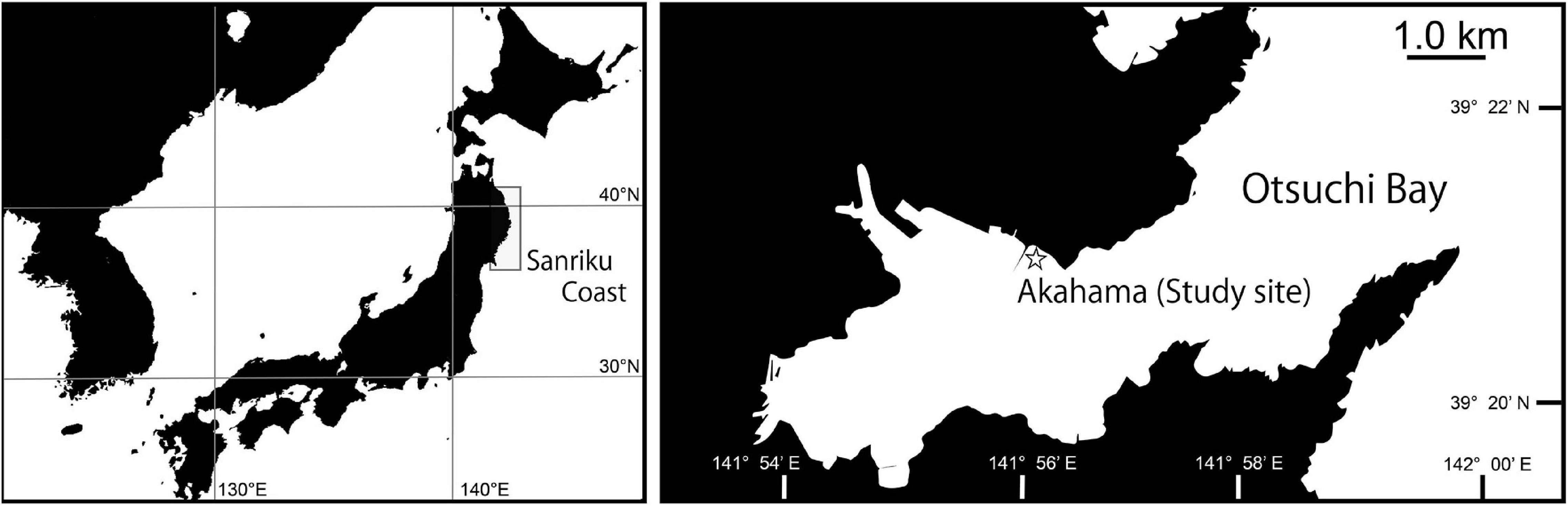
Figure 1. The survey site was located on the subtidal rocky shore in Otsuchi Bay, Japan. The shaded area indicates the area of Sanriku Coast, and the star symbol indicates the location of the survey site.
Obtaining Image Sequences
At the study site, five sections (A01 to A05) were chosen from the part of the bedrock surface for obtaining image sequences. The horizontal projected areas of the five sections were 11.3–25.5″, and they were located at 1.5–5.0 m depth. For each section, 89–178 photos were taken from various angles using SCUBA equipment (Figures 2A–C). Overlap rates between two consecutive photos were more than 70%. Photos were taken using a waterproof digital camera Tough TG-5 OLYMPUS with a wide-angle lens. The camera was set to the underwater wide mode, and no flash was used. Large seaweeds sway in the waves and veil the surface of the bedrocks so that the construction of 3D models was difficult when dense large seaweeds occur. In the study site, annual seaweeds Ulva spp., Desmarestia virdis (Müller) Lamouroux, 1813, and Undaria pinnatifida (Harvey) Suringar, 1872 dominated and they grew from winter to summer. Therefore, we conducted the field survey during November 2018 when large seaweeds were detached and the bedrock surface were exposed. Photographing was conducted at the daytime when the current was calm, the water clarity was high, and strong shadows did not occur.
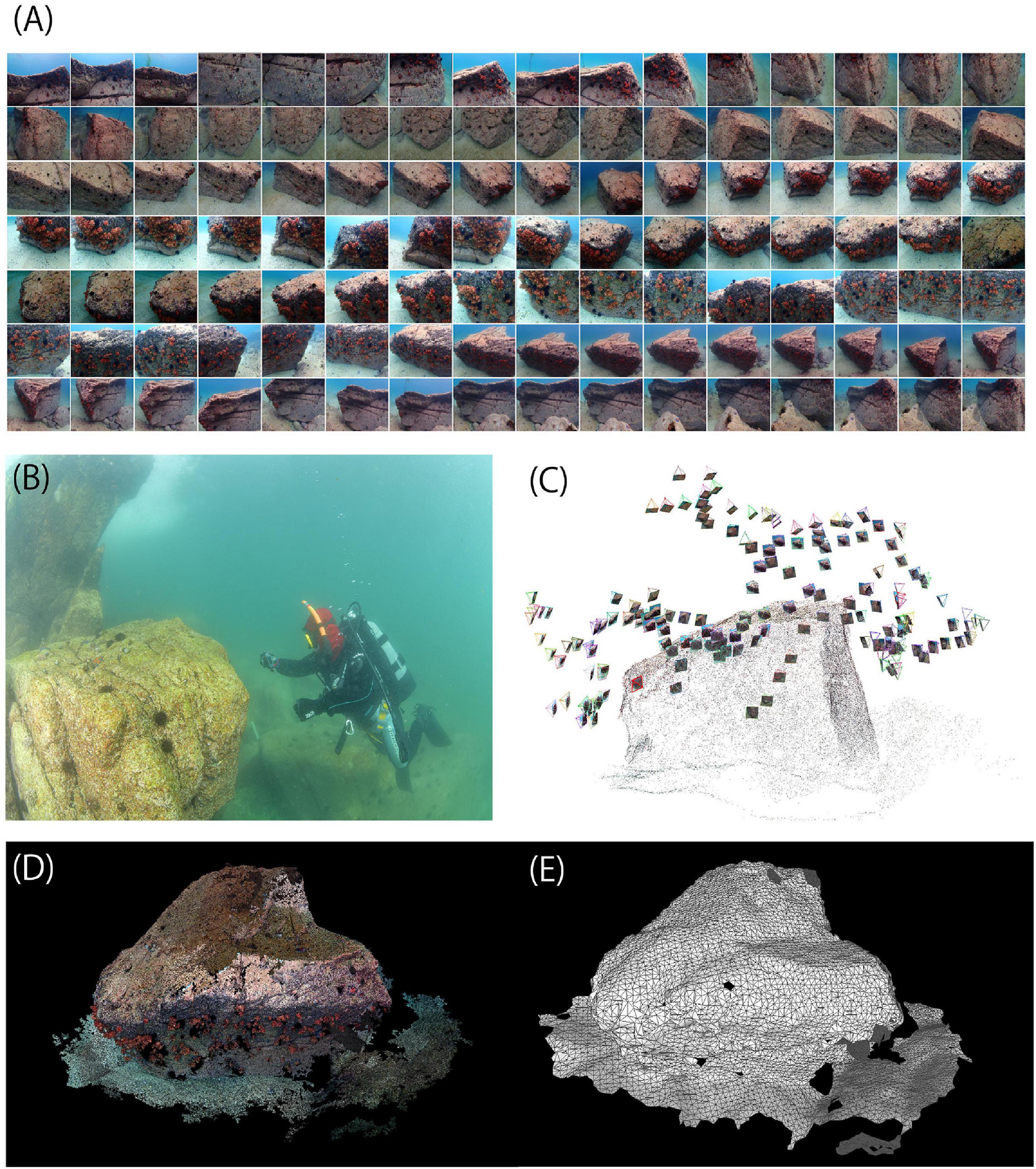
Figure 2. Figures of the 3D seafloor topographic model construction process. (A) Image sequences of the section A01. (B) The scene of survey by SCUBA diving. (C) Locations of each photo estimated by Visual SfM. (D) The 3D point cloud model reconstructed from image sequences. (E) 0.05 m resolution mesh model translated by Meshlab.
On each bedrock surface for surveying, a reference point where the slope is 0 degree was found with a clinometer. At the reference point, the depth and azimuth were measured using a depth meter of the digital camera Tough TG-5 and an azimuth magnetic needle, respectively. In addition, for setting the size of the 3D models, a 20 cm square frame was placed at this point and a photograph was taken from a distance that can distinguish the location of the reference point on the 3D model.
3D Model Construction From Image Sequences
The 3D structure of each rock was reconstructed using the Visual SfM v0.5.26, an open-source software (Wu et al., 2011; Wu, 2013) that implements the Structure from Motion (SfM) algorithms. Visual SfM reconstructs the 3D structure from continuous overlapping image sequences (Figure 2D). Uploading the images to the Visual SfM, the tools Pairwise Matching, Reconstruct Sparse, and Reconstruct Dense were executed. The 3D model constructions were conducted using a HP Workstation with 32 GB memory and 1 GB GPU.
Meshing of the 3D Models
The obtained 3D point cloud models (Figure 3) were converted to 0.01 m resolution point cloud models and 0.05 m resolution mesh models. The 3D point cloud models constructed by Visual SfM were deployed using MeshLab 2016.12, an open-source software. The x-axis, y-axis, and z-axis directions were set to north, east, and vertical upward based on the value of the azimuth magnetometer taken at the reference point. The length 1.0 of the 3D models was set to 1.0 m based on the 20 cm square frame photograph taken at the reference point. The resolution of the obtained point cloud models differed both among rocks and within rocks because the quality of each image was different due to the variation of brightness.
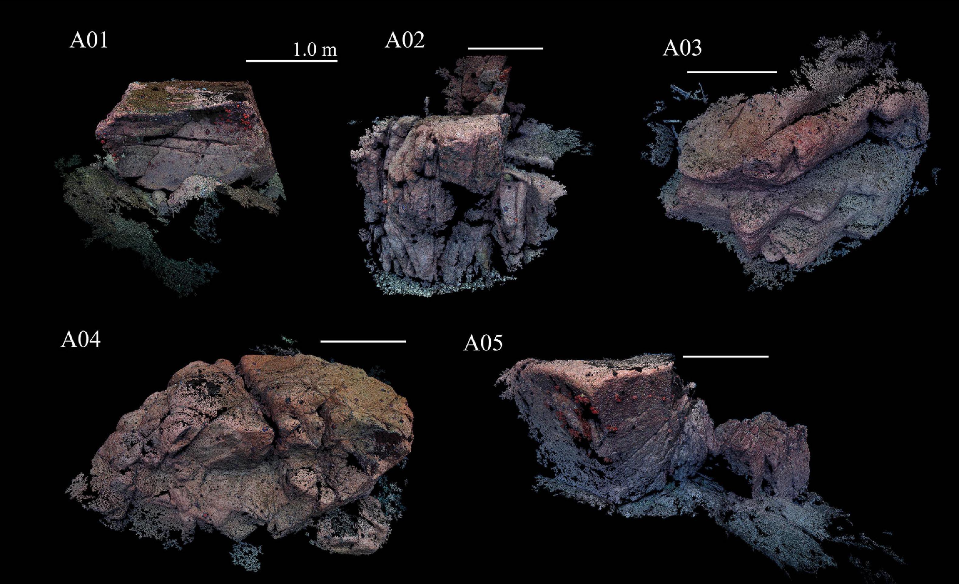
Figure 3. 3D seafloor topographic models of the five sections of the subtidal rocky shores in Otsuchi Bay, Japan.
The point cloud models were equalized to the 0.01 m and 0.05 m resolution models using the “Clustered Vertex Subsampling” tool setting “Cell size” as 0.01 and 0.05. The 0.05 m resolution point cloud models were converted to the triangular irregular network (TIN) mesh models using the “Surface Reconstruction: Ball Pivoting” tool (Figure 2E). In general, 3D point cloud models of seafloor topography are converted to raster models in which elevation values are stored for each grid of the x-y plane, but raster models are prone to be rough for the near-vertical plane due to rapid changes in elevation (Kemp, 2007). Therefore, TIN models were used in order to handle bedrock surfaces including near-vertical planes. The directions of the faces were calculated by the “Compute normal for point sets” tool. Some faces were incorrectly directed back from the actual front sides. The incorrectly directed faces were manually flipped in MeshLab.
Due to shadows in the photos and low resolution of the obtained 3D point cloud models, some areas in the 3D mesh models were missing. Because the missing areas were smaller than 10% of the total models and the number of sessile organisms on these areas was small, we ignored these areas and conducted the subsequent analysis.
Input of the Presence/Absence Data of Sessile Organisms
Four sessile species, a solitary ascidian Halocynthia roretzi (Drasche, 1884), a barnacle Balanus trigonus Darwin, 1854, a tube-forming polychaete Paradexiospira nakamurai Uchida, 1971, and an articulated coralline alga Pachyarthron cretaceum (Postels and Ruprecht) Manza, 1937 were dominant on the surface of bedrock in the study site (Figure 4). Three sessile animals H. roretzi, B. trigonus, and P. nakamurai are suspension feeder.
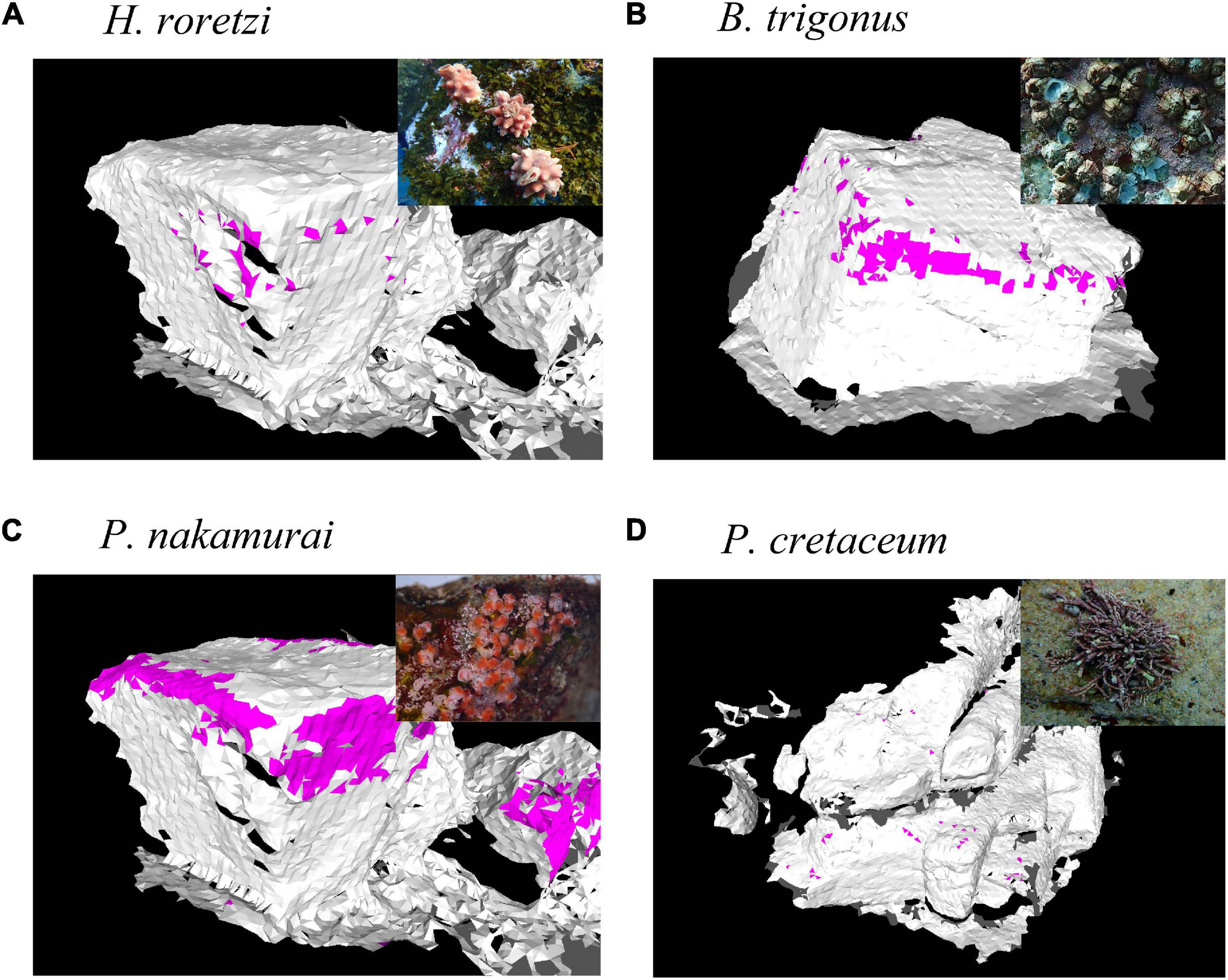
Figure 4. Examples of occurrence data of sessile organisms. Colored faces indicate the faces each species occurred. (A) Halocynthia roretzi, (B) Balanus trigonus, (C) Paradexiospira nakamurai, (D) Pachyarthron cretaceum.
In preliminary samplings, we caught and identified the sessile species dominated in the study site. Presence/absence data of each species were added to the 3D mesh models (Figure 4). Species and the location of each individual were identified from the photos which were also used for photogrammetry. In H. roretzi and P. cretaceum, as their diameters were larger than 5 cm, the presence data on a face of the two species is equivalent to the occurrence of one individual. In P. nakamurai and B. trigonus, as their diameters were smaller than 1 cm and they are gregarious species, the presence data on a face of the two species can include multiple individuals. This data included the location of dead individuals of B. trigonus, as the presence of the empty shell still indicates that the area was suitable for barnacle growth.
Calculating the Terrain Variables
On all the faces of each 0.05 m resolution mesh model, seven terrain variables; height above seafloor (as height), topological position index (as TPI), northness, eastness, 360 degrees azimuth (as aspect), as well as slope, and ruggedness were calculated based on the vertices of the 0.01 m resolution point cloud models (Figure 5). The vertices set of 0.01 m are denoted by V0.01={vm|vm ∈ R3}(m=1,…m0.01). vm=(xm,ym,zm) is the coordinates of the m-th vertice. m0.01 is the number of vertices V0.01. The vertices and faces set of the 0.05 m resolution mesh models are denoted by and T0.05={tn|tn⊂V0.05}(n=1,…n0.05), respectively. m0.05 is the number of vertices of the mesh model V0.05, and n0.05 is the number of the faces of the mesh model T0.05. Because we used triangular faces, the elements of each face are represented as tn=(v1n,v2n,v3n),(vin∈V0.05), using three vertices that constitute the face. The following terrain variables were calculated by Python3.7.3.
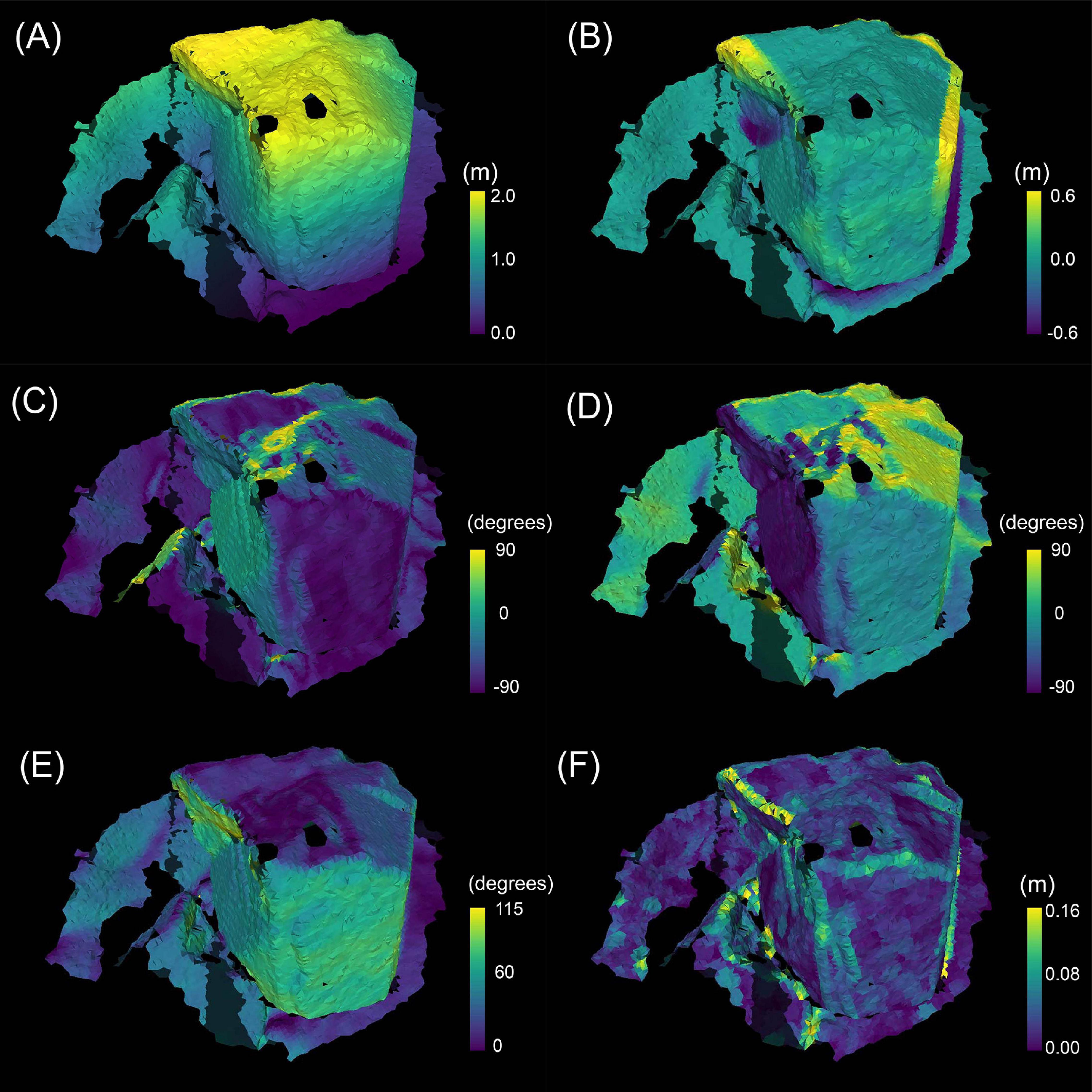
Figure 5. The terrain variables calculated on the 3D mesh model of site A01. The brightness of the color indicates the magnitude of each variable. (A) height above the seafloor (height), (B) topological position index (TPI), (C) slope, (D) aspect (northness), (E) aspect (eastness), (F) ruggedness.
Height Above Seafloor (Height)
Height is a parameter of the height above the seafloor. The seafloor was defined as the lowest z-value point in each mesh model. In each mesh model, the lowest z-value point is denoted by min(zm). The center of gravity coordinates on the target face tnis denoted by . Height is calculated in meters as subtracting z_G with min(zm), i.e.:
Topological Position Index (TPI)
TPI is an index of the height above or below the mean height of surroundings defined by a specific neighborhood (Weiss, 2001). A positive TPI value indicates the z-axis directional convex terrain, such as ridges or peaks. In contrast, a negative TPI value indicates the z-axis directionally recessed terrain, such as a valley or depression. TPI values near zero are either flat or constant slope areas. The vertices in the circle around t_G with radius Rm are referred to as V_R. TPI is calculated in meters as subtracting z_G with the mean z-value of V_R, that is z_R i.e.:
Northness, Eastness, and 360 Degrees Azimuth (Aspect)
360 degrees azimuth were splitted to northward component (northness) and eastward component (eastness). V_R was fit to the plane DR:ax + by + cz + d=0. The coefficients a, b, c, and d were calculated by the method of least squares of the V_R. Northness, Eastness, and 360 degrees azimuth (aspect) were calculated using the normal of the D_R. The normal of the D_R was denoted by nDR=(nx,ny,nz). The direction of the normal was specified with the front and back direction of the target face. Since the x-axis direction was specified as east, the y-axis direction as north,
Northness and eastness take the value from -90 to 90. The combination of northness and eastness gives a 360 degrees azimuth. For example, (northness, eastness) = (90, 0) indicates that it is facing north, while (northness, eastness) = (−90, 0) indicates facing south. The 360 degrees azimuth were defined as 0 degrees north, 90 degrees east, 180 degrees south, and 270 degrees west.
Slope
0 degree in slope indicates the horizontal plane, 90 degree indicates vertical plane, and 180 degree indicates overhang plane. Slope was also calculated using the normal of the D_R. Slope is calculated as the following equation:
Ruggedness
Ruggedness was the parameter of the unevenness of the terrain. Ruggedenss was defined as the difference of the maximum height above or maximum depth below the plane D_R. Ruggedness was calculated in meters with the following equation:
vi means the coordinates of the i-th vertex and means the average coordinates of the VR.
The small scale of the topographic survey resulted in 3D topographic models including the shape of the organisms themselves. This may have resulted in a significant error in the values of the terrain variables, especially in faces where large H. roretzi and seaweeds were present. A practicable solution for this problem is to take a sufficiently wide computational range of R to obtain the terrain variables. In this study, TPI, slope and aspect were calculated in the range of 0.10 m, and ruggedness was calculated in the range of 0.20 m for detecting a wide range of topographic changes. This allowed us to represent topographic changes on a scale larger than the size of the organisms surveyed in this research.
Statistical Analysis
Correlation Analysis Between Terrain Variables
The correlations between terrain variables (height, TPI, northness, eastness, slope, and ruggedness) were calculated by Pearson’s linear correlation coefficient (LCC), and maximal information coefficient (MIC). MIC is the non-linear correlation coefficient based on the mutual information criteria between two variables. MIC can detect complex variable relationships, whereas LCC can detect only linear relationships (Speed, 2011).
In order to reduce the calculation time, the randomly 50% extracted data of terrain variables were used in calculating MIC. LCC and MIC were computed by Python 3.7.3 with the library scipy1.2.1, and minepy1.2.4, respectively.
Comparison of the Occurrence Conditions Among Species
For each variable (height, TPI, northness, eastness, slope, and ruggedness), the difference of occurrences pattern between species (including background data) was examined. Background data means the terrain variables obtained in the whole 3D models. As the normality of all the distributions was rejected by Shapiro-Wilk’s test (p < 0.01) and therefore, the difference of occurrence pattern between species were examined by the multiple comparison with Mann-Whitney U test. As multiple comparisons were made, the significance level was reduced from 0.05 to 0.005 (=0.05/10) to adjust for 10 multiple comparisons (Bonferroni procedure). These statistical tests were conducted by the library scipy1.2.1 with Python3.7.3.
Contribution of Each Terrain Variable to Occurrence of Sessile Organisms
The contribution rate of each terrain variable for the four sessile organisms was estimated by the jackknife test with maximum entropy modeling which is the machine learning method for modeling species geographic distributions with presence-only datasets (Phillips et al., 2006). We used MaxEnt version 3.4.1, a software that implements the maximum entropy modeling for estimating the contribution rate of each parameter. MaxEnt was applied using linear features, quadratic features, and product features for each terrain variable. MaxEnt outputs the contribution rate of each terrain variable as the regularized training gain by the jackknife test. Simultaneously, the performance of the maximum entropy model was evaluated using the area under the curve (AUC) derived from the threshold independent receiver operating characteristics (ROC) curves.
Results
3D Model Construction
Figure 3 shows the 3D models of the five sections of the bedrock surfaces constructed using photogrammetry. The point cloud models constructed using SfM (raw model) were composed of more than 1.5-million points (Table 1). The raw models were converted to 0.01 m resolution point cloud models composed of 290–520 thousand points and 0.05 m resolution mesh models composed of 13–42 thousand points and 25–42 thousand faces.
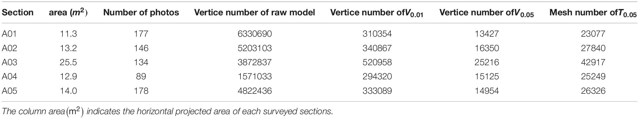
Table 1. Properties of the 3D models at five surveyed sections (A01–A05).
Correlation of Terrain Variables
Figure 6 shows the Pearson’s linear correlation coefficients (LCC) and mutual information criteria (MIC) between terrain variables. Aspect is divided into northness and eastness. The maximal value of LCC was 0.45, which was recorded between height and TPI. The maximal value of MIC was 0.78 between northness and eastness. The values of MIC were lower than 0.16 among height, TPI, slope, and ruggedness.
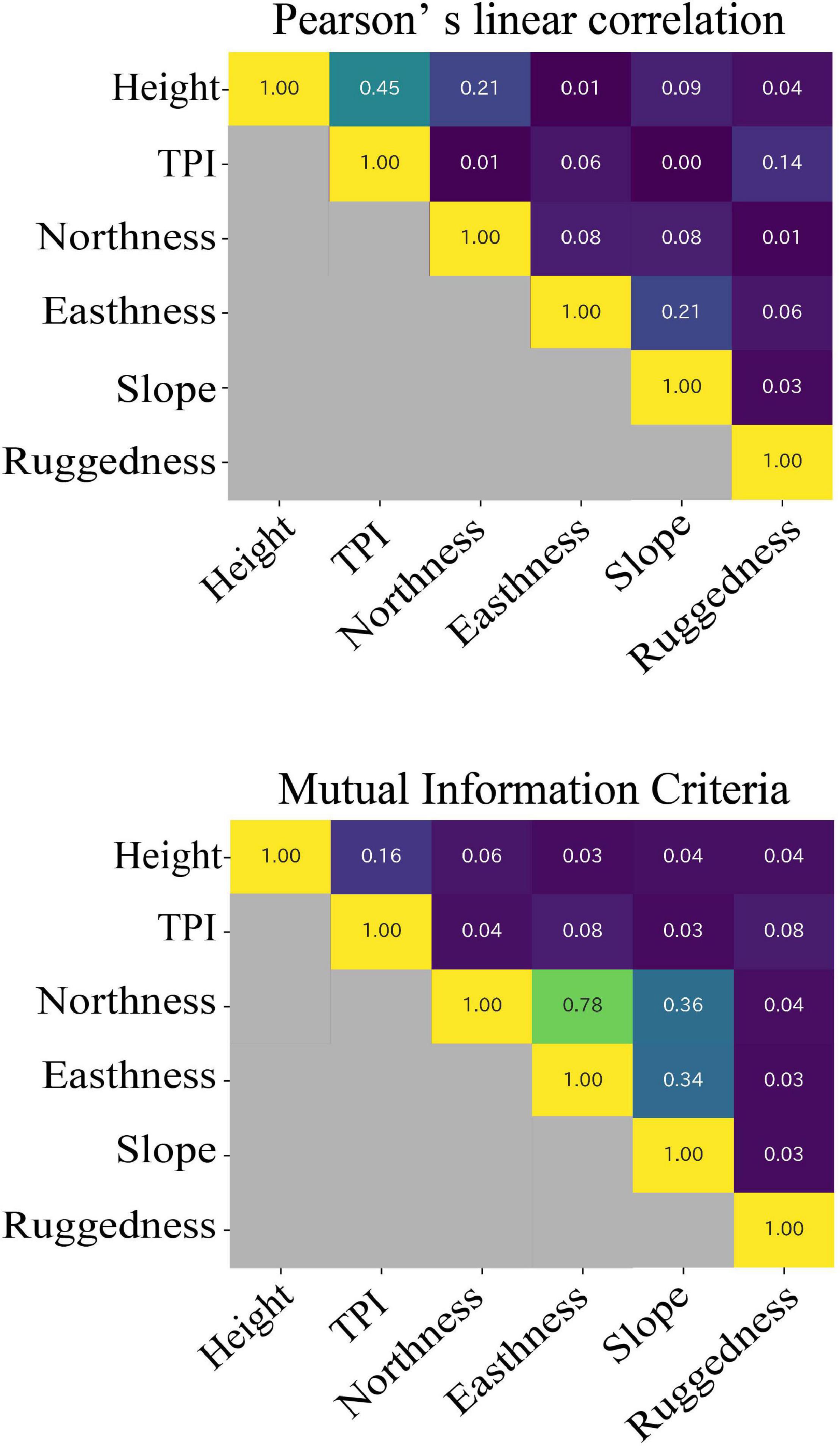
Figure 6. Results of Pearson’s linear correlation coefficients (LCC) and maximal information coefficients (MIC).
Species Occurrences
The total number of faces where at least one species of sessile organisms occurred was 9,522. Paradexiospira nakamurai was the dominant sessile organisms and occurred on 5,293 faces. The species compositions differed among the surveyed sections. Halocynthia roretzi occurred on all the surveyed sections, but the occurrences of H. roretzi was low on A02, A03, and A04. Pachyarthron cretaceum also occurred on all the surveyed sections. Balanus trigonus did not occur on A03 and A04, and P. nakamurai did not occur on A01 and A04 (Table 2).
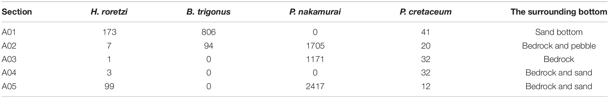
Table 2. The numbers of faces on which each species occurred at each section (A01–A05) and surrounding bottoms.
Species Distribution and Terrain Variables
Height
In all the surveyed bedrocks (background), the maximum value of the height was 3.9 m. More than 95% of H. roretzi, B. trigonus, and P. nakamurai occurred on 1.0–3.0 m height. P. cretaceum occurred on the surface areas higher than 0.3 m height, and 95% of them occurred at 0.5–3.0 m height. P. cretaceum distribution height range was wider than those of the three sessile animals (Figure 7). The median height where P. nakamurai occurred was 2.1 m, which was higher than values for the other species (Figure 8), and significant differences between P. nakamurai and the other species as well as background were detected by the multiple comparison with Mann-Whitney U test (p < 0.005, Table 3). For all species, the densities of occurrences showed similar patterns to the number of occurrences (Figure 7).
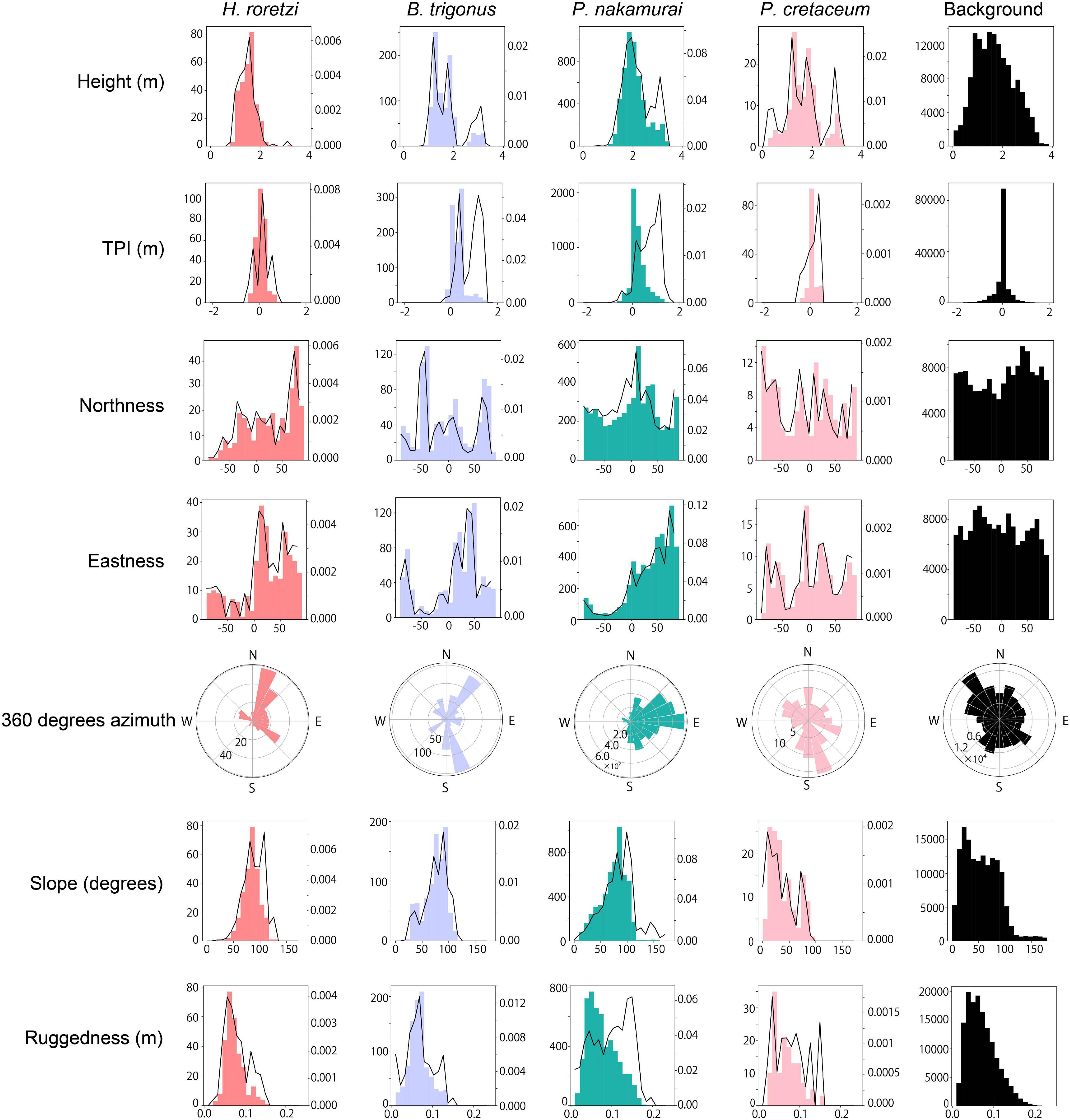
Figure 7. Relationships between each terrain variable (height, TPI, northness, eastness, 360 degrees azimuth, slope, and ruggedness) and the occurrences of each species. For each parameter and each species, the number of occurrences is shown in histograms. Except for 360 degrees azimuth, the density of the occurrences was shown in line plots, which is the number of occurrences divided by the number of each bin of the background histogram. The horizontal axis refers to the value of each terrain variable, the left side of the vertical axis refers to the number of occurrences, and the right side of the vertical axis refer to the density of the occurrences which is the number of occurrences divided by the number of background in each bin. In aspects, the r direction refers to the number of occurrences and the θ direction refers to the aspect.
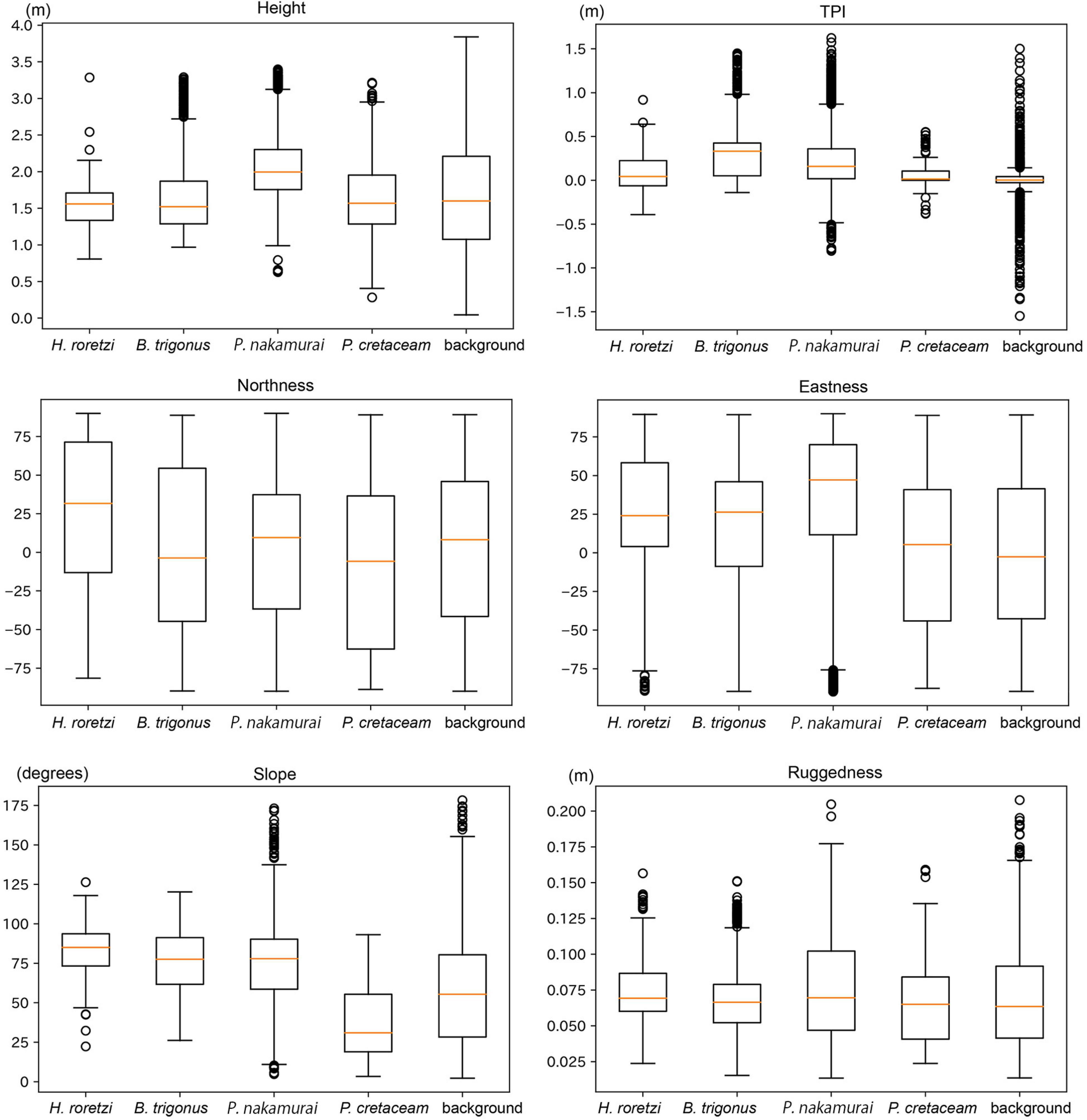
Figure 8. Boxplots of terrain variables of the faces where each species occurred. Boxplots show the range (solid black lines), median (red lines), 25 and 75% quantiles (box), and outliers at 95% confidence (points).

Table 3. P-values of the multiple comparison with the Mann-Whitney test.
TPI
In all the surveyed bedrocks, TPI ranged -2.1 to 2.0. TPI distributed symmetrically from the center of 0.0 in all the surveyed bedrocks. More than 75% of H. roretzi, B. trigonus, and P. nakamurai occurred on the position with positive values of TPI. More than 80% of P. cretaceum occurred in the range -0.2 to 0.2 TPI (Figure 7). In all the species, the median TPIs where each species occurred was larger than the median TPI of the background (Figure 8), and significant difference between the four species and background was detected by the multiple comparison with Mann-Whitney U test (p < 0.005, Table 3). The densities of occurrences of H. roretzi showed similar patterns to the number of occurrences. Two peaks, around 0.0 and 1.0, were observed in the densities of occurrences of B. trigonus. In P. nakamurai and P. cretaceum, peaks were found around 1.0 and 0.5, respectively, in the densities of occurrences, which were larger than the mean values of the numbers of occurrences (Figure 7).
Aspect
In all the surveyed bedrocks, northeast faces were slightly dominant. The numbers of occurrences of H. roretzi were higher on northern faces, and that of B. trigonus was higher on northern and southwestern faces. Large numbers of P. nakamurai occurred on northeastern faces, and they rarely occurred on western faces. Most P. cretaceum occurred on southeastern faces (Figure 7). The median northness of the faces where H. roretzi occurred, and the median eastness of the faces where P. nakamurai occurred were higher than those of the other species (Figure 8). Significant differences between H. roretzi and the other species in northness were detected using the multiple comparison with Mann-Whitney U test (p < 0.005, Table 3). Significant differences between P. nakamurai and the other species in eastness were detected using the multiple comparison with Mann-Whitney U test (p < 0.005, Table 3). For all species, the densities of occurrences showed similar patterns to the numbers of occurrences (Figure 7).
Slope
In all the surveyed bedrocks, there were two peaks around near-horizontal approximately 30 and near-vertical approximately 90 degrees in the slope distribution. In terms of the three sessile animals, H. roretzi, B. trigonus, and P. nakamurai, there were peaks in the 70–100 degrees slope. H. roretzi distribution slope range was wider than those of B. trigonus and P. nakamurai (Figure 7). These species also occurred on an overhanging faces > 90 degrees. In P. cretaceum, there was a peak in the 10–20 degrees slope. No P. cretaceum occurred on the position with overhang faces >90 degrees (Figure 7). The median slope of the faces where P. cretaceum occurred was less than those of the other species (Figure 8). Significant differences between them were detected by the multiple comparison with Mann-Whitney U test (p < 0.005, Table 3). For all species, the densities of occurrences showed similar patterns to the numbers of occurrences (Figure 7).
Ruggedness
In all the surveyed bedrocks, the ruggedness ranged from 0.01 to 0.24 (Figure 7). H. roretzi and P. nakamurai occurred on higher ruggedness faces than B. trigonus and P. cretaceum (Figure 8). Significant differences between them were detected by the multiple comparison with Mann-Whitney U test (p < 0.005, Table 3). In B. trigonus, the peak of ruggedness (0.66–0.70) was the highest in all species. In P. nakamurai, the peak of the densities of occurrences was 0.14, which was higher than that of the numbers of occurrences. In the other three species, the densities of occurrences showed similar patterns to the number of occurrences (Figure 7).
The Combination of Multiple Conditions
The parallel coordinates were used to visualize the combinations of terrain variables with high occurrences and the interactions between variables (Figure 9). H. roretzi and B. trigonus were abundant in areas of more than 1.0 m height above the seafloor, on steep slopes of 45–120 degrees, and on various degrees of aspect and ruggedness. P. nakamurai was more abundant in areas of more than 1.0 m height above the seafloor and on various degrees of slope, aspect and ruggedness. P. cretaceum was more abundant on 0–60 degrees slope, southwestern faces, and various heights.
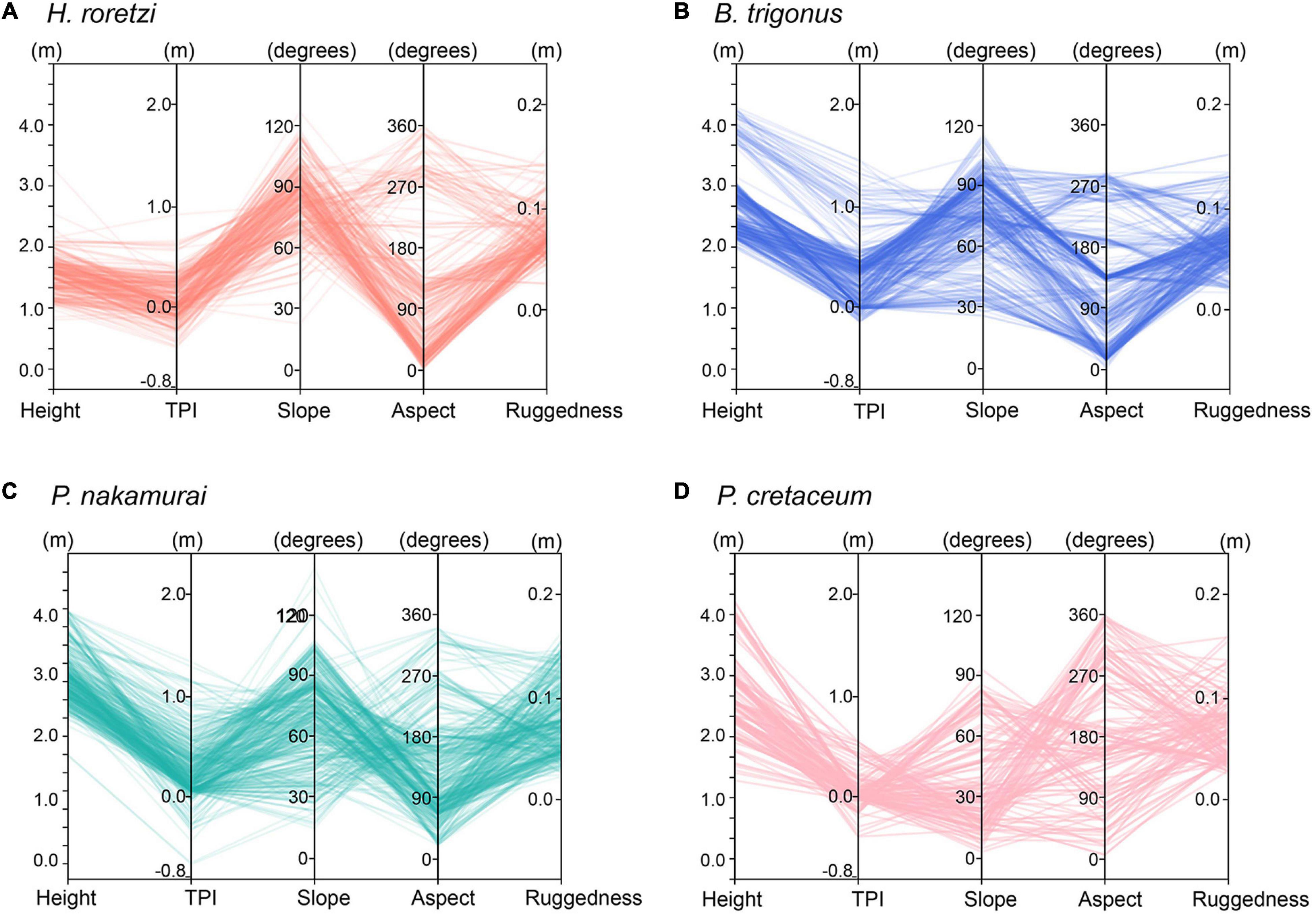
Figure 9. Parallel coordinate graphs showing the combinations of terrain variables which each species of sessile organisms occurred [(A) H. roretzi (B) B. trigonus (C) P. nakamurai (D) P. cretaceum]. In parallel coordinates, each terrain variable at the location where an individual occurred is connected by a single plot. Respective lines indicate individual faces each species occurred. This allowed us to visualize not only the distribution of each terrain variable, but also the combinations of terrain variables with high occurrences.
Contribution of Each Terrain Variable
For H. roretzi and P. cretaceum, the contribution of slope was the largest, followed by height in H. roretzi, and TPI in P. cretaceum (Figure 10). For B. trigonus, the contribution of TPI was the largest, followed by slope. For P. cretaceum, the contribution of height was the largest, followed by TPI. In H. roretzi and B. trigonus, the AUCs of training data were 0.922 and 0.897, respectively. In P. cretaceum and P. nakamurai, the AUCs of training data were 0.792 and 0.762, respectively, which were lower than those of other two species.
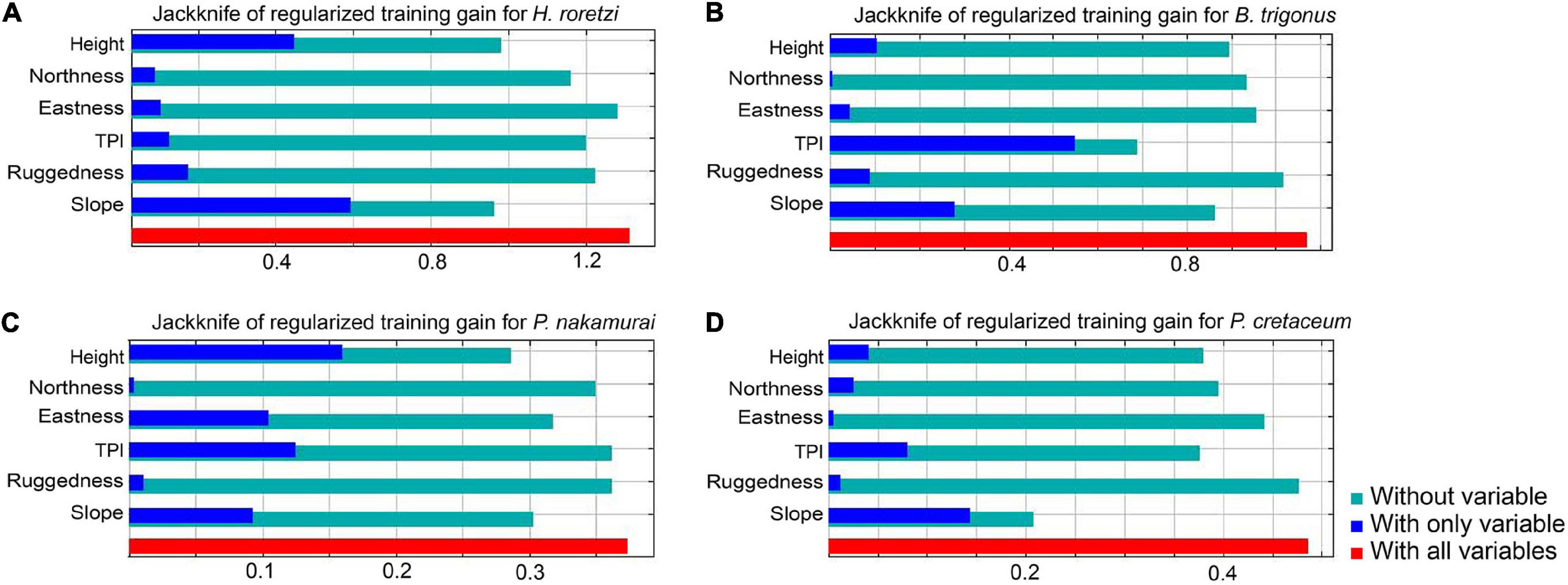
Figure 10. Jacknife of regularized training gain for (A) H. roretzi, (B) B. trigonus, (C) P. nakamurai, (D) P. cretaceum. The lengths of the bars “With all variables” represent the full model accuracies with all parameters. Those of “Without variables” represent the model accuracies in which each variable was excluded. Those of “With only variables” represent the accuracies of the model in which only each variable was used, and effectively shows the contribution rate for explaining the presence or absence of the distribution.
Discussion
Seafloor Topographic Surveying Methods
In the present study, we succeeded in measuring multiple terrain variables of the subtidal rocky shore using underwater photogrammetry. In conventional field measurement methods, the ability to obtain detail of multiple terrain variables on a lot of points has been limited. Therefore, the relationships between the distribution of sessile organisms and terrain variables have been investigated only at the meter-scale with side-scan sonar or multibeam sonar (Wilson et al., 2007; Dolan et al., 2008; Tong et al., 2013; Georgian et al., 2014; Miyamoto et al., 2017). The resolution of the 3D seafloor topographic models obtained in the present study is much more detailed (0.05 meter-resolution) than those in the acoustic-based methods, which enabled us to investigate the distribution patterns of sessile organisms using more detailed scale of terrain variables.
To implement the photogrammetry method in other sites, it should be noted that the resolution of photos is affected by the transparency of the water. At sites with insufficient brightness light, photos need to be taken using flash. In addition, to choose seasons when there are no large seaweeds swaying in the waves.
The photogrammetry method in the present study can measure terrain variables even on the entire model, resulting in an analysis of bedrock topography more accurate than those based on conventional field measurement methods. For example, in the study site, two peaks near horizontal and vertical slope were observed. This may indicate the topographic characteristics of the granite cliff (Dale, 1923), the fracture surface of which is prone to plane orthogonally (cleavage), resulting in a block shaped bedrock (Figure 7).
Distribution patterns of each species based on 0.01 meter-scale terrain variables will be essential information for predicting what species occur on what kind of topographies (biological habitat mapping) in shallow marine rocky shores. In deep waters, biological habitat mapping has been conducted mainly for setting up the protect areas of cold-water corals from the bottom trawling fishery (Wilson et al., 2007; Dolan et al., 2008; Tong et al., 2013; Georgian et al., 2014; Miyamoto et al., 2017). In the shallow waters, the seafloor topography is often simplified by human activities. Topological simplifications significantly affect diversity and biomass of sessile organism communities (Perkol-Finkel et al., 2006). The species richness of sessile organisms often decreases on the artificial reefs of which the centimeter scale topography is simple (Loke and Todd, 2016). The communities of sessile organism play important roles for ecosystems on the subtidal rocky shore, such as habitat, food, spawning substrate, and shelter for other benthic organisms in coastal areas (Sarà, 1986). Seaweeds are also important as primary producers (Dean and Connell, 1987). Therefore, maintaining the biomass and the diversity of sessile organisms are important. To predict the decrease of sessile organisms by topographic alterations and to find the measures for conservation of the sessile organisms, the detailed scale habitat suitability modeling using photogrammetry may greatly contribute.
Habitat Suitability of Sessile Organisms
By analysis using multiple terrain variables, the combination of terrain variables of the faces on which each species occurred was elucidated. This enable more accurate distribution patterns of sessile organisms than those obtained in conventional studies focusing on one or two terrain variables. For example, occurrences of barnacles and ascidians were previously detected to be more on vertical planes than on horizontal planes (Wendt et al., 1989; Connell, 1999). The present study revealed that the number of the ascidian Halocynthia roretzi and the barnacle Balanus trigonus were large at high and vertical planes, and small at low positions, even on vertical planes.
The most important terrain variable for habitat preference varied with species. These variables were height (height above the seafloor and TPI) or slope. These variables may indicate the physical environment, such as light intensity and the current velocity. At steep slopes and high positions above the seafloor, the numbers of the three species of sessile animals (H. roretzi, B. trigonus, and the tube-forming polychaete Paradexiospira nakamurai) were higher than at low positions. Simulations and experiments of the currents around artificial reefs have shown that the presence of topographic abrupt changes cause contractions of the current flow and upwellings (Su et al., 2007; Liu and Su, 2013). In the case study on the artificial reefs about 20 m wide and 10 m high, the wake vortex flow arises behind the artificial reefs due to the contraction. Due to upwelling and backflow vortex, high densities of plankton have been shown to locally form on the upper part of the artificial reefs (Yanagi and Nakajima, 1991). Even on small, natural bedrocks in the subtidal rocky shore, since the depth which rapid becomes shallow is similar to that of the case study, the upwellings may arise and increase the food supply at high positions above the seafloor.
Therefore, on vertical planes at high positions, a large amount of particles may pass through due to the exposure to the contractions and the backflow vortex, which results in the favorable environment for suspension feeders. Conversely, at low positions on horizontal and vertical planes, obtaining food may be difficult for suspension feeders due to stagnant currents. Suspended materials close to the seafloor may also hinder feeding and growth of sessile suspension feeders (Robbins, 1983).
Most of H. roretzi occurred on north, vertical and middle height (lower than 2 m height) faces (Figures 7, 8), therefore H. roretzi might prefer the place with low light intensity. In addition, the southwestern wave direction excelled in the study site. Therefore, the contraction frequently may occur on the north and vertical faces, and these faces might well be favorable environment for H. roretzi feeding. Most of H. roretzi, B. trigonus, and P. nakamurai occurred on high ruggedness convex and concave surfaces (Figures 7, 8), which may function as refuges from predators like starfishes, sea urchins, and gastropods. In convex areas, the flow velocity increases due to the generation of turbulence. The feeding pressure on kelps by sea urchins is known to decrease in high current velocities (Kawamata, 2010). In concave areas, predators like large starfishes, sea urchins, and fish are prevented from access (Menge and Lubchenco, 1981). These phenomena may decrease the feeding pressure on sessile animals by predators in convex and concave areas. The articulated coralline alga, Pachyarthron cretaceum is not a suspension-feeder unlike the sessile animals, and therefore may occur even at lower heights and ruggedness faces than other suspension-feeding animals. More P. cretaceum occurred at a height over 1.0 m above the seafloor on southeastern near-horizontal faces, which will be suitable for their photosynthesis due to higher light intensities. Sea urchins more favorably prey on sessile animals than articulated coralline algae which have a low nutritional value for sea urchins (Endo et al., 2007). The low feeding pressure on P. cretaceum by sea urchins may be one of the factors allowing them to grow at low heights and ruggedness faces where the current velocities are moderate and feeding by sea urchins was minimal.
In order to detail the precise factors regulating the distribution of sessile organisms, elucidating how terrain variables are specifically indicative of the physical and biological environments is needed. However, investigating the relationships between topographic conditions and physical environments is a frontier that has not been considered for rocky reef ecosystems, which could be carried by the development of numerical simulations and measurements of flow speed and light availability.
Although the distribution ranges were different among four sessile species, the occurrence conditions were similar and overlapped among three sessile animals H. roretzi, B. trigonus, and P. nakamurai. However, the number of occurrences at the peak of each species was much smaller than (less than 1/10) the number of background data. For example, the number of P. nakamurai occurrences peaked approximately 1,000 faces at 81–90 degrees, and the number of background data at 81–90 degrees was approximately 10,000 faces. Therefore, in the study site, there were surplus suitable habitat, suggesting that the sessile species were not under intense competition and they occurred in accordance with their habitat preferences.
In each terrain variable except TPI, the number and the density of occurrences showed similar patterns in all species. The peaks of the number of occurrences may indicate the suitable habitat conditions for each species. In TPI, for three sessile species except H. roretzi, the peaks of the density of occurrences were higher than those of the number of occurrences (Figure 7). Therefore, high TPI faces may be more suitable for the inhabitation of B. trigonus, P. nakamurai, and P. cretaceum than moderate TPI faces. High TPI faces may be under competition among those three species, and therefore, the number of occurrences may be higher on moderate TPI faces than on high TPI faces.
The species compositions of sessile organisms were different among the five sections of the bedrocks surface. The occurrences of H. roretzi, B. trgionus, and P. nakamurai became more concentrated in specific section of the bedrock surface. The communities of sessile organisms in the intertidal zone are known to be affected by the priority effect: when the substrate became vacant, the species of which a lot of larvae exist can settle on and dominate the substrates (Connell, 1961). The same effect may have caused biases of the species occurrences among sections. In addition, some species of barnacles have been reported to attach close to the adult individuals of the same species (Knight-Jones and Stevenson, 1950; Crisp and Meadows, 1962), which may result in the bias of the occurrences among sections.
In addition, the parameters not obtained in the photogrammetry method, such as the distance from the shore, distribution of the surrounding sediments or the terrain variables calculated on meter scales can possibility affect the species occurrences. For example, the distribution of P. nakamurai may be affected by aspects on a wider scales. The surveyed sections “A02,” “A03,” and “A05” were located on the east side of rocky shore of the study site, and therefore were composed of mainly east faces at the sufficiently larger scale than 0.1 m. P. nakamurai only occurred on these sections. Although the reason for this occurrence pattern is unknown, this may be related to the fact that east side of the rocky shore in the study site was susceptible to the effects of southwestern wave direction. Relationships between the surrounding sediment of each section and the species occurrence were not detected (Table 2). Although we focused only on centimeter-scale terrain variables in this study, coarse and broad scale topographic surveying by echo sounder is also necessary in order to investigate these wider scale environmental conditions. By combining narrow but detailed methods by photogrammetry and coarse but wide methods, we will get better ecological understandings about habitat suitability of various sessile organisms.
Conclusion
In the present study, 3D seafloor topographic models with 0.05 m resolution were constructed using photogrammetry on subtidal rocky shore, and the relationships between distributions of sessile organisms and multiple terrain variables calculated from the 3D models were successfully investigated.
Distributions of each species were found to be affected by multiple terrain variables, such as height, TPI, aspect, slope, and ruggedness. High height above the seafloor was important for the distributions of three species of sessile animals, and gentle slope was important for that of an articulated coralline alga, P. cretaceum. The light intensity and flow conditions controlled by these terrain variables might affect the distribution of each species.
As measuring the multiple terrain variables was difficult with conventional direct measurement methods, the effects of topography on the distribution of sessile organisms have not received much attention in spite of their underlying importance. In the present study, we developed a new method to investigate the relationships between the distribution of sessile organisms and multiple terrain variables, which can provide more accurate information of habitat suitable conditions for each species than the previous studies conducted on subtidal rocky shores.
Data Availability Statement
The raw data supporting the conclusions of this article will be made available by the authors, without undue reservation, to any qualified researcher.
Author Contributions
TKan conducted all the field survey and data analysis, also developed the analytical methods, and drafted the manuscript. JH planned the field surveys. KN joined the field surveys. KN and JH helped to draft the manuscript. TKit and TKaw supervised this study. All authors discussed the results and approved the submitted version of the manuscript.
Funding
This work was supported by the Sasakawa Scientific Research Grant (2018-7020) and the Tohoku Ecosystem-Associated Marine Sciences project.
Conflict of Interest
The authors declare that the research was conducted in the absence of any commercial or financial relationships that could be construed as a potential conflict of interest.
Acknowledgments
We greatly thank Masaaki Hirano, Takanori Suzuki, Nobuhiko Iwama, Naoya Otsuchi, Masafumi Kodama, and other members of International Coastal Research Center, Atmosphere and Ocean Research Institute, The University of Tokyo, Masato Hirose (Kitasato University), and Kaito Fukuda (Fukuda Marine Research Diving) for supporting surveying in Otsuchi Bay. We also thank Eijiroh Nishi (College of Education Yokohama National University) for supporting identification of polychaete.
References
Agudo-Adriani, E. A., Cappelletto, J., Cavada-Blanco, F., and Cróquer, A. (2019). Structural complexity and benthic cover explain reef-scale variability of fish assemblages in Los Roques National Park, Venezuela. Fron. Mar. Sci. 6:690. doi: 10.3389/fmars.2019.00690
Archambault, P., and Bourget, E. (1996). Scales of coastal heterogeneity and benthic intertidal species richness, diversity and abundance. Mar. Ecol. Prog. Ser. 136, 111–121. doi: 10.3354/meps136111
Barnes, H., Crisp, D. J., and Powell, H. T. (1951). Observations on the orientation of some species of barnacles. J. Anim. Ecol. 20, 227–241. doi: 10.2307/1542
Bayley, D. T. I., Mogg, A. O. M., Koldewey, H., and Purvis, A. (2019). Capturing complexity: field-testing the use of ‘structure from motion’ derived virtual models to replicate standard measures of reef physical structure. PeerJ 7:e6540. doi: 10.7717/peerj.6540
Bryson, M., Ferrari, R., Figueira, W., Pizarro, O., Madin, J., Williams, S., et al. (2017). Characterization of measurement errors using structure-from-motion and photogrammetry to measure marine habitat structural complexity. Ecol. Evol. 7, 5669–5681. doi: 10.1002/ece3.3127
Burns, J. H. R., Delparte, D., Gates, R. D., and Takabayshi, M. (2015). Utilizing underwater three-dimensional modeling to enhance ecological and biological studies of coral reefs. Int. Arch. Photogramm. Remote Sens. Spat. Inf. Sci. XL-5/W5, 61–66. doi: 10.5194/isprsarchives-XL-5-W5-61-2015
Chabot, R., and Bourget, E. (1988). Influence of substratum heterogeneity and settled barnacle density of the settlement of cypris larvae. Mar. Biol. 97, 45–56. doi: 10.1007/BF00391244
Chase, A. L., Dijkstra, J. A., and Harris, L. G. (2016). The influence of substrate material on ascidian larval settlement. Mar. Pollut. Bull. 106, 35–42. doi: 10.1016/j.marpolbul.2016.03.049
Chiba, S., and Noda, T. (2000). Factors maintaining topography-related mosaic of barnacle and mussel on a rocky shore. J. Mar. Biol. Assoc. U. K. 80, 617–622. doi: 10.1017/S0025315400002435
Connell, J. H. (1961). The influence of interspecific competition and other factors on the distribution of the barnacle Chthamalus Stellatu. Ecology 42, 710–723. doi: 10.2307/1933500
Connell, S. D. (1999). Effects of surface orientation on the cover of epibiota. Biofouling 14, 219–226. doi: 10.1080/08927019909378413
Courtney, L. A., Fisher, W. S., Raimond, S., Oliver, L. M., and Davis, W. P. (2007). Estimating 3-dimensional colony surface area of field corals. J. Exp. Mar. Biol. Ecol. 351, 234–242. doi: 10.1016/j.jembe.2007.06.021
Crisp, D. J., and Barnes, H. (1954). The orientation and distribution of barnacles at settlement with particular reference to surface contour. J. Anim. Ecol. 23, 142–162. doi: 10.2307/1664
Crisp, D. J., and Meadows, P. S. (1962). The chemical basis of gregariousness in cirripedes. Proc. R. Soc. B 156, 500–520.
Dean, R. L., and Connell, J. H. (1987). Marine invertebrates in an algal succession. III. Mechanisms linking habitat complexity with diversity. J. Exp. Mar. Biol. Ecol. 109, 249–273. doi: 10.1016/0022-0981(87)90057-8
Dolan, M. F. J., Grehan, A. J., Guinan, C., and Brown, C. (2008). Modelling the local distribution of cold-water corals in relation to bathymetric variables: adding spatial context to deep-sea video data. Deep Sea Res. 55, 1564–1579. doi: 10.1016/j.dsr.2008.06.010
Endo, H., Nakabayashi, N., Agatsuma, Y., and Taniguchi, K. (2007). Food of the sea urchins Strongylocentrotus nudus and Hemicentrotus pulcherrimus associated with vertical distributions in fucoid beds and crustose coralline flats in northern Honshu, Japan. Mar. Ecol. Prog. Ser. 352, 125–135. doi: 10.3354/meps07121
Fallati, L., Saponari, L., Savini, A., Marchese, F., Corselli, C., and Galli, P. (2020). Multi-temporal UAV data and object-based image analysis (OBIA) for estimation of substrate changes in a post-bleaching scenario on a Maldivian reef. Remote Sens. 12:2093. doi: 10.3390/rs12132093
Friedman, A., Pizarro, O., Williams, S. B., and Johnson-Roberson, M. (2012). Multi-scale measures of rugosity, slope and aspect from benthic stereo image reconstructions. PLoS One 7:e50440. doi: 10.1371/journal.pone.0050440
Georgian, S. E., Shedd, W., and Cordes, E. E. (2014). High-resolution ecological niche modelling of the cold-water coral Lophelia pertusa in the Gulf of Mexico. Mar. Ecol. Prog. Ser. 506, 145–161. doi: 10.3354/meps10816
Hirose, M., and Kawamura, T. (2017). Distribution and seasonality of sessile organisms on settlement panels submerged in Otsuchi Bay. Coast. Mar. Sci. 40, 66–81. doi: 10.15083/00074036
Hughes, R. G. (1975). The distribution of epizoites on the hydroid Nemertesia antennina (L.). J. Mar. Biol. Assoc. U. K. 55, 275–294. doi: 10.1017/S0025315400015940
Johnson, M. P., Frost, N. J., Mosley, M. W. J., Roberts, M. F., and Hawkins, S. J. (2003). The area-independent effects of habitat complexity on biodiversity vary between regions. Ecol. Lett. 6, 126–132. doi: 10.1046/j.1461-0248.2003.00404.x
Kawamata, S. (2010). Inhibitory effects of wave action on destructive grazing by sea urchins: a review. Bull. Fish. Res. Agency 32, 95–102.
Kemp, K. (ed.) (2007). Encyclopedia of Geographic Information Science. Thousand Oaks, CA: SAGE publications, Inc.
Keough, M. J., and Downes, B. J. (1982). Recruitment of marine invertebrates: the role of active larval choices and early mortality. Oceologia 54, 348–352. doi: 10.1007/BF00380003
Kim, K., Lecours, V., and Frederick, P. C. (2018). Using 3d micro-geomorphometry to quantify interstitial spaces of an oyster cluster. PeerJ Prepr. 7:e27596v1. doi: 10.7287/peerj.preprints.27596v1
Knight-Jones, E. W., and Stevenson, J. P. (1950). Gregariousness during settlement in the barnacle Elminius modestus Darwin. J. Mar. Biol. Assoc. U. K. 29, 281–297.
Knott, N. A., Underwood, A. J., Chapman, M. G., and Glasby, T. M. (2006). Growth of the encrusting sponge Tedania anhelans (Lieberkuhn) on vertical and on horizontal surfaces of temperate subtidal reefs. Mar. Freshw. Res. 57, 95–104. doi: 10.1071/MF05092
Komatsu, K., and Tanaka, K. (2017). Swell-dominant surface waves observed by a moored buoy with a GPS wave sensor in Otsuchi Bay, a ria in Sanriku, Japan. J. Oceanogr. 73, 87–101. doi: 10.1007/s10872-016-0362-4
Leichter, J. J., and Witman, J. D. (1997). Water flow over subtidal rock walls: relation to distributions and growth rates of sessile suspension feeders in the Gulf of Marine water flow and growth rates. J. Exp. Mar. Biol. Ecol. 209, 293–307. doi: 10.1016/S0022-0981(96)02702-5
Leon, J. X., Roelfsema, C. M., Saunders, M. I., and Phinn, S. R. (2015). Measuring coral reef terrain roughness using ‘Structure-from-Motion’ close-range photogrammetry. Geomorphology 242, 21–28. doi: 10.1016/j.geomorph.2015.01.030
Liu, T. L., and Su, D. T. (2013). Numerical analysis of the influence of reef arrangements on artificial reef flow fields. Ocean Eng. 74, 81–89. doi: 10.1016/j.oceaneng.2013.09.006
Loke, L. H. L., and Todd, P. A. (2016). Structural complexity and component type increase intertidal biodiversity independently of area. Ecology 97, 383–393.
Lozano-Cortés, D. F., and Zapata, F. A. (2014). Invertebrate colonization on artificial substrates in a coral reef at Gorgona Island, Colombian Pacific Ocean. Rev. Biol. Trop. 62, 161–168. doi: 10.15517/rbt.v62i0.16273
Menge, B. A., and Lubchenco, J. (1981). Community organization in temperate and tropical rocky intertidal habitats: prey refuges in relation to consumer pressure gradients. Ecol. Monogr. 51, 429–450. doi: 10.2307/2937323
Miyamoto, M., Kiyota, M., Murase, H., Nakamura, T., and Hayashibara, T. (2017). Effects of bathymetric grid-cell sizes on habitat suitability analysis of cold-water gorgonian corals on seamounts. Mar. Geodesy 40, 205–223. doi: 10.1080/01490419.2017.1315543
Otobe, H., Onishi, H., Inada, M., Michida, Y., and Terazaki, M. (2009). Estimation of water circulation in Otsuchi Bay, Japan inferred from ADCP observation. Coast. Mar. Sci. 33, 78–86. doi: 10.15083/00040706
Paine, R. T. (1966). Food web complexity and species diversity. Am. Nat. 100, 65–75. doi: 10.1086/282400
Perkol-Finkel, S., Shashar, N., and Benayahu, Y. (2006). Can artificial reefs mimic natural reef communities? The roles of structural features and age. Mar. Environ. Res. 61, 121–135. doi: 10.1016/j.marenvres.2005.08.001Get
Phillips, S. J., Anderson, R. P., and Schapire, R. E. (2006). Maximum entropy modeling of species geographic distributions. Ecol. Modell. 190, 231–259. doi: 10.1016/j.ecolmodel.2005.03.026
Pizarro, O., Friedman, A., Bryson, M., Williams, S. B., and Madin, J. (2017). A simple, fast, and repeatable survey method for underwater visual 3D benthic mapping and monitoring. Ecol. Evol. 7, 1770–1782. doi: 10.1002/ece3.2701
Ponti, M., Perliini, R. A., Ventra, V., Grech, D., Abbiati, M., and Cerrano, C. (2014). Ecological shifts in Mediterranean coralligenous assemblages related to gorgonian forest loss. PLoS One 9:e102782. doi: 10.1371/journal.pone.0102782
Robbins, I. J. (1983). The effects of body size, temperature, and suspension density on the filtration and ingestion of inorganic particulate suspensions by ascidians. J. Exp. Mar. Biol. Ecol. 70, 65–68. doi: 10.1016/0022-0981(83)90149-1
Robert, K., Huvenne, V. A. I., Georgiopoulou, A., Jones, O. B., Marsh, L., Carter, G. D. O., et al. (2017). New approaches to high-resolution mapping of marine vertical structures. Sci. Rep. 7:9005. doi: 10.1038/s41598-017-09382-z
Sanford, E., and Menge, B. A. (2001). Spatial and temporal variation in barnacle growth in a coastal upwelling system. Mar. Ecol. Prog. Ser. 209, 143–157. doi: 10.3354/meps209143
Sarà, M. (1986). Sessile macrofauna and marine ecosystem. Ital. J. Zool. 53, 329–337. doi: 10.1080/11250008609355518
Smith, F. G. W. (1946). Effect of water currents upon the attachment and growth of barnacles. Biol. Bull. 90, 51–70. doi: 10.2307/1538061
Smith, J., O’Brien, P. E., Stark, J. S., Johnstone, G. J., and Riddle, M. J. (2015). Integrating multibeam sonar and underwater video data to map benthic habitats in an East Antarctic nearshore environment. Estuar. Coast. Shelf Sci. 164, 520–536. doi: 10.1016/j.ecss.2015.07.036
Speed, T. (2011). A correlation for the 21st century. Science 334, 1502–1503. doi: 10.1126/science.1215894
Su, D. T., Liu, T. L., and Ou, C. H. (2007). A comparison of the PIV measurements and numerical predictions of the flow field patterns within an artificial reef. Paper Presented at the 17th International Offshore and Polar Engineering Conference, Vol. 1–4, Lisbon, 2239–2245.
Thomason, J. C., Hills, J. M., Clare, A. S., Neville, A., and Richardson, M. (1998). Hydrodynamic consequences of barnacle colonization. Hydrobiologia 375/376, 191–201. doi: 10.1023/A:1017088317920
Tong, R., Purser, A., Guinan, J., and Unnithan, V. (2013). Modeling the habitat suitability for deep-water gorgonian corals based on terrain variables. Ecol. Inf. 13, 123–132. doi: 10.1016/j.ecoinf.2012.07.002
Weiss, A. D. (2001). “Topographic positions and landforms analysis (poster),” in Poster at the ESRI International User Conference, San Diego, CA: ESRI.
Wendt, P. H., Knott, D. M., and Van Dolah, R. F. (1989). Community structure of the sessile biota on five artificial reefs of different ages. Bull. Mar. Sci. 44, 1106–1122.
Westoby, M. J., Brasington, J., Glasser, N. F., Hambrey, M. J., and Reynolds, J. M. (2012). ‘Structure-from-Motion’ photogrammetry: a low-cost, effective tool for geoscience applications. Geomorphology 179, 300–314. doi: 10.1016/j.geomorph.2012.08.021
Wilson, M. F. J., O’Connell, B., Brown, C., Guinan, J. C., and Grehan, A. J. (2007). Multiscale terrain analysis of multibeam bathymetry data for habitat mapping on the continental slope. Mar. Geodesy 30, 3–35. doi: 10.1080/01490410701295962
Wu, C. (2013). “Towards linear-time incremental structure from motion,” in Proceedings of the 2013 International Conference on 3D Vision – 3DV 2013, Seattle, WA, 127–134. doi: 10.1109/3DV.2013.25
Wu, C., Agarwal, S., Curless, B., and Seitez, S. M. (2011). “Multicore bundle adjustment,” in Proceedings of the CVPR 2011, Colorado Springs, CO, 3057–3064. doi: 10.1109/CVPR.2011.5995552
Yanagi, T., and Nakajima, M. (1991). Change of oceanic condition by the man-made structure for upwelling. Mar. Pollut. Bull. 23, 131–135. doi: 10.1016/0025-326X(91)90662-C
Keywords: topographic features, benthic communities, habitat suitability modeling, rocky shore ecology, Sanriku Coast
Citation: Kanki T, Nakamoto K, Hayakawa J, Kitagawa T and Kawamura T (2021) A New Method for Investigating Relationships Between Distribution of Sessile Organisms and Multiple Terrain Variables by Photogrammetry of Subtidal Bedrocks. Front. Mar. Sci. 8:654950. doi: 10.3389/fmars.2021.654950
Received: 18 January 2021; Accepted: 01 March 2021;
Published: 29 March 2021.
Edited by:
Javier Xavier Leon, University of the Sunshine Coast, AustraliaReviewed by:
Xihan Mu, Beijing Normal University, ChinaMarilia Bueno, State University of Campinas, Brazil
Hirokazu Abe, Iwate Medical University, Japan
Giovanni Coletti, Milano Bicocca University, Italy
Copyright © 2021 Kanki, Nakamoto, Hayakawa, Kitagawa and Kawamura. This is an open-access article distributed under the terms of the Creative Commons Attribution License (CC BY). The use, distribution or reproduction in other forums is permitted, provided the original author(s) and the copyright owner(s) are credited and that the original publication in this journal is cited, in accordance with accepted academic practice. No use, distribution or reproduction is permitted which does not comply with these terms.
*Correspondence: Takayuki Kanki, dGthbmtpQGFvcmkudS10b2t5by5hYy5qcA==