Global Oceanic Eddy Identification: A Deep Learning Method From Argo Profiles and Altimetry Data

The inadequate spatial resolution of altimeter results in low identification efficiency of oceanic eddies, especially for small-scale eddies. It is well known that eddies can not only induce sea surface signal but more importantly have typical vertical structure characteristics. However, although the vertical structure characteristics are usually used for statistical analysis, they are seldom considered in the process of eddy recognition. This study is devoted to identifying eddies from the perspective of their vertical signal derived from the 18-year Argo data. Due to the irregular and noisy profile pattern, the direct identification of eddy core from Argo profile is deemed to be a challenge. With the popularity of artificial intelligence, a new hybrid method that combines the advantages of convolutional neural network (CNN) with extreme gradient boosting (XGBoost) is proposed to extract the representative vertical feature and identify eddy from a profile. First, CNN is employed as a feature extractor to automatically obtain vertical features from the input profile at the bottom of the network. Second, the obtained high-dimensional feature vectors are inputted into the XGBoost model, combined with other profile features for classifying profiles that are outside altimeter-identified eddies (Alt eddy). Finally, extensive experiments are implemented to demonstrate the efficiency of the proposed method. The results show that the classification accuracy of CNN-XGBoost model can reach 98%, and about 36% eddies are recaptured. These eddies, dubbed CNN-XGB eddies, are benchmarked against Alt eddies for the vertical structure and geographical distribution, demonstrating a similar or even stronger vertical signal and a prominent eddy belt in the tropical ocean. Within the proposed theory framework, there are various potentials to obtain a better outlook for eddy identification and in situ float observations.

Introduction

Ocean eddies are omnipresent and play a significant role in transporting water mass, heat, and nutrients since their capacity of trapping fluid parcels and generate vertical movements within their cores, effectively impacting the ocean’s circulation, large-scale water distribution, and biology (Bryden and Brady, 1989; Chelton et al., 2011a,b; Faghmous et al., 2012; Zhang et al., 2014; Amores et al., 2018).

Oceanic eddy detection is a key step in promoting the development of eddy science, which has been widely studied based on the variety of remote sensing data. The current mainstream eddy recognition method based on an automatic algorithm from gridded maps of sea level anomaly (SLA) is proved to be an effective method (Chelton et al., 2011b; Faghmous et al., 2015; Le Vu et al., 2018). Although the merged dataset is enabling observational studies of mesoscale features [with a spatial resolution of (1/4)° and a temporal resolution of daily] that were not previously possible using altimetry data (e.g., ∼315 km at the equator of the TOPEX/Poseidon), the limitation of satellite altimeter dataset in spatial resolution is still proven to be too large to resolve the two-dimensional of oceanic eddies (Fu et al., 2010), especially the oceanic eddies with a diameter smaller than 50 km. Amores et al. (2018) concluded that eddy recognition method based on sea surface height is largely underestimating the density of eddies; capturing only between 6 and 16% of the total number of eddies due to the limited resolution of the altimeter gridded products is not enough to capture the small-scale eddies that are the most abundant. Besides, some studies have tried to identify eddies from other sea surface characteristics. For instance, Gonzalez-Silvera et al. (2004) effectively identified and tracked 18 eddies in the tropical Pacific Ocean using 5 months of SeaWiFS and AVHRR data. D’Alimonte (2009) used sea surface temperature (SST) data to iterate the SST isotherm for automatic eddy detection. However, eddy detection using SST is prone to false positives because many other ocean phenomena also impact the sea surface temperature and surface ocean color (chlorophyll concentration) (Du et al., 2018). While the eddy detection based on the SAR principle has a high resolution and a small coverage area that can identify submesoscale or even small-scale eddies, it is easily affected by the wind field on the sea surface. Besides, many studies have shown that eddies also sometimes present as subsurface phenomena that are not noticeable by snapshots from satellite altimetry or other satellite sensors, leading to detecting uncertainties (Jeronimo and Gomez-Valdes, 2007; Andrade et al., 2014; Zhang et al., 2014; Gordon et al., 2017).

The sign of temperature/salinity anomalies inside individual eddies occurs due to geostrophic uplift and depression of the background pycnocline vertical profiles associated with eddies (Dong et al., 2012). Compared with 1–30 cm amplitude of the sea surface caused by eddies, the ∼1,000 m seawater anomaly amplitude below the sea surface caused by them cannot be ignored. The main part of the eddy should be considered as the underwater position where the largest seawater density anomaly occurs or in other words, the eddy core. It is more stable than the eddy features mapped to the sea surface and is not limited by the spatial resolution of satellite remote sensing. Its strength and depth directly determine the eddy energy and is the key to the study of eddy dynamics and thermodynamics. In this way, eddies, especially small eddies, weak eddies, subsurface eddies, etc., which cannot be detected by remote sensing, can be identified by their three-dimensional structure characteristics. With the development of the Argo global network, studies on the vertical structure of eddy have been enriched and developed. Recently, it has been effectively proved that we can derive the vertical distribution caused by eddies as criteria for anticyclonic eddies (AE)/cyclonic eddies (CE) identification through a training–learning process using concurrent altimeter-Argo measurements at a given location and then scanning all Argo profiles outside altimetrically derived eddies according to the setup criteria to locate missing eddies (Chen et al., 2020). However, the shape of an eddy’s vertical structure is complex, regionally susceptible, and polarity controlled. For example, by collocating historical records of Argo profiles and satellite altimetry data, Chaigneau et al. (2011) reconstructed the mean 3-D eddy structure in the eastern South Pacific Ocean and suggested that the core (maximum temperature and salinity anomalies in the vertical direction) of CE is centered at ∼150 m below the surface, while the core of AE is centered at ∼400 m. Dong et al. (2012) shed light on three types of eddies’ vertical shapes: bowl shaped (with the largest radius at the surface), lens shaped (with the largest radius at the middle), and cone shaped (with the largest radius at the bottom) based on high-resolution numerical model product. Pegliasco et al. (2015) analyzed different eddy vertical shapes by using clustering analysis in four major Eastern Boundary Upwelling Systems. These existing studies have a common conclusion, that is, the vertical shapes of oceanic eddies are not spatially and timely uniform, and the eddy cores of AE and CE are asymmetric even if they are in the same region. Moreover, these eddy structures were obtained through the composite superposition or multiprofile averaged, which were relatively smooth and regular. But in general, an original eddy profile will present a more irregular and noisy profile pattern making it a challenge to seek out the eddy core directly. Consequently, the application of artificial intelligence will be the expecting method to extract the representative feature of each profile for eddy identification.

Deep-learning algorithms, which learn the representative and discriminative features hierarchically from the data, have been becoming a hotspot and have been introduced into the geoscience community for big data analysis. Considering the low-level features as the bottom level, the output feature representation from the top level of the network can be directly fed into a subsequent classifier for pixel-based classification (Zhang et al., 2016). Convolutional neural network (CNN) is an efficient deep learning model with hierarchical structure to learn high-quality features at each layer. Since the model can reduce the complexity of network structure and the number of parameters through local receptive fields, weight sharing, and pooling operation, and can actively extract high-dimensional features from big data as well, it is a suitable model that can be used to extract profile feature information. Although CNN has been recognized as one of the most powerful and effective mechanisms for feature extraction, traditional classifiers connected to CNN cannot fully understand the extracted features (Ren et al., 2017). Boosting is one of the most prominent classification techniques in the state-of-the-art, providing the best accuracy levels at many problems. However, the most known boosting algorithm, AdaBoost, has already been proven to be sensitive against noise. Since Chen’s proposal of the extreme gradient boosting (XGBoost) model (Chen and Guestrin, 2016), the theory and application of the decision tree method have developed significantly. This model is proven to be the most robust algorithm in both binary and multiclass datasets for its strong resolution of data noise, fast calculation speed, and high accuracy and has been widely employed in various classification applications. Inspired by the above facts, we aimed to develop a novel hybrid CNN-XGBoost model for fully learning the profile features. This composite model can provide more accurate classification results by regarding CNN as a trainable feature extractor to automatically obtain features from the input profile and XGBoost as a recognizer and combined with other remarkable profile features in the top level of the network to produce results.

This paper aims to propose a new perspective to identify eddies from vertical structure characteristics with deep learning architecture. The objective of this paper is mainly twofold: one is the hybrid CNN-XGBoost architecture construction for vertical characteristics extraction, and the other is the comparison and verification of the obtained eddy dataset. This is a significant step forward compared to previous studies that focused only on “sea surface characteristics of eddies” for identification. Such an unprecedented improvement in state-of-the-art spatial–temporal sampling and coverage of the Argo project allows us to obtain a unique and massive dataset of subsurface T/S records. The rest of the paper is organized as follows: In Data, we describe the two datasets (altimetry and Argo data) used in this work, and the eddy identification algorithm based on satellite data is briefly presented. Methods introduces the methods, including the dataset preprocessing principles, CNN model, and XGB model principles and architecture along with the experimental environment. The results are presented in Results. The global eddy vertical structure characteristics are described in Global Eddy Vertical Structure Characteristics. Model Training Process explains the training process and accuracy evaluation of the model. In Eddy Identification Based on CNN-XGBoost Model, both the vertical structure and geographical distribution characteristics of identified eddies by our method are analyzed in detail. Additionally, a concise result on the relationship between eddy property and its vertical structure is presented in Vertical Structure of CNN-XGB Eddy. Finally, Conclusions contains a brief discussion and our conclusions.

Data

Satellite Altimeter Data

The sea level anomaly (SLA) data used in this study is delayed time products generated by Archiving, Validation, and Interpretation of Satellite Oceanographic (AVISO) from a combination of T/P, Jason-1, Jason-2, Jason-3, and Envisat missions. The SLA dataset spanned 18 years, from January 2002 to October 2019, and had a daily temporal resolution and a (1/4)° × (1/4)° spatial resolution. In the present analysis, a four-step scheme has been optimized for eddy identification based on our earlier work by Liu et al. (2016). First, a high-pass filtering is applied to the global SLA data using a Gaussian filter with a zonal radius of 10° and a meridional radius of 5° before seed points are effectively determined. Second, the global SLA fields are divided into regular blocks with a zonal spacing of 45° and a meridional spacing of 36°. Third, SLA contours are computed with a 0.25-cm interval, and eddy boundaries corresponding to maximum geostrophic velocity are subsequently extracted. Finally, all blocks are merged seamlessly into a global map with duplicated eddies eliminated. Following the identification schemes, a comprehensive eddy dataset has been created for the global ocean, which is available at http://coadc.ouc.edu.cn/tfl/ and http://data.casearth.cn/ (Data ID: XDA19090202), and relevant technical details (including models and procedures) can be found in Liu et al. (2016), Sun et al. (2017), and Tian et al. (2020).

Argo Floats

The Array for Real-time Geostrophic Oceanography (Argo) data also spanned from January 2002 to October 2019. The Argo project is the first global observation system for the subsurface ocean and is one of the best sources for in situ temperature measurements. Argo floats observe large temporal (seasonal and longer) and spatial (thousand kilometers and larger) scale subsurface ocean variability worldwide (Roemmich et al., 2009). At present, Argo is collecting ∼12,000 data profiles each month (∼400 a day). This greatly exceeds the amount of data that can be collected from below the ocean surface by any other method. By September 21, 2020, there are as many as 3910 active floats disseminated around the global ocean spacing nominally at every 3° of longitude and latitude. In this analysis, the Argo floats data are provided by the Coriolis Global Data Acquisition Center of France through their website: www.coriolis.eu.org. The quality control and processing of Argo data are conducted automatically by the Argo data center, and only profiles flagged as “good” or “probably good” are downloaded. Meanwhile, additional data filtering is applied to profiles with first measurement shallower than 10 m and last measurement deeper than 1,000 m and meanwhile having at least 30 valid data points within the 0–1,000 m depth range. Finally, linear interpolation with an interval of 1 m is carried out for all edited high-quality profiles in the global ocean.

Since density is a combination of temperature and salinity, it can comprehensively evaluate the vertical structure anomalies caused by eddies. Therefore, in this paper, the potential density anomaly (PDA) is chosen as the property to represent the vertical structure of eddies for eddy identification. After preprocessing and filtering the profile data, the potential density is calculated based on International Thermodynamic Equation of Seawater 2010 from Argo T/S profile data using the Gibbs Seawater Oceanographic toolbox (McDougall et al., 2009), and anomalies of every profile are computed by removing climatological profiles. Here, the climatological T/S profiles are obtained by interpolating the CSIRO Atlas of Regional Seas to floats’ positions and times (Dunn and Ridgway, 2002; Ridgway et al., 2002).

Materials and Methods

Data Preprocessing for Different Types of Eddies

We established our dataset starting from the Argo profiles data. Based on the positions and times of eddies and Argo floats, Argo profiles are classified into three categories depending on whether the floats are inside the effective boundaries (i.e., the outermost enclosed contour of SLA surrounding the eddy centroid) of the altimeter recognized eddies (Alt eddy) or outside eddies. The numbers of profiles that fall inside anticyclonic eddies (Alt AE) or cyclonic eddies (Alt CE) in this study are 343,802 and 328,936, respectively, and 1,271,784 profiles are outside Alt eddies. Figure 1 shows the geographical distribution of Argo profiles. In general, the patterns of these figures are determined by the locations where the Argo floats are gathered such as the Kuroshio extension, the Arabian Sea, and the North Atlantic. However, compared with Figures 1b,c, it can be found that the Argo profile inside Alt eddy only accounts for about one-third of the total profile (Figure 1b). Two-thirds of profiles are outside the Alt eddy (Figure 1c). However, whether these profiles are actually outside the eddy or actually inside the eddy but just not captured by the altimeter needs to be determined by their vertical structure characteristics.

FIGURE 1

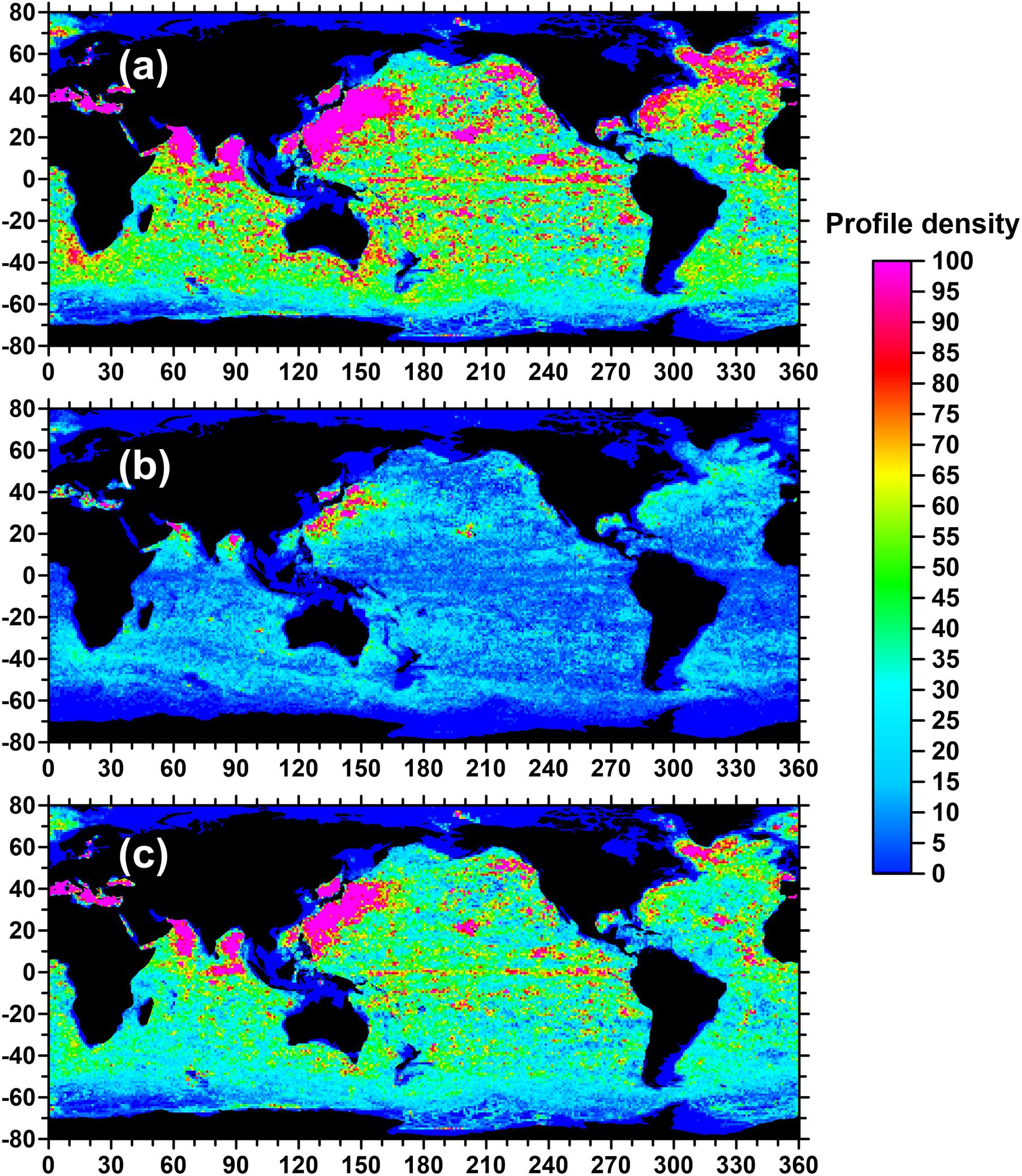
Figure 1. Global geographic distribution of Argo profiles during 2002–2019 under 1° × 1° grid. (a–c) Cumulative number of all profiles, profiles inside Alt eddies, and profiles outside Alt eddies, respectively.

There is a part of the eddies that are identified by the altimeter as cyclonic (anticyclonic) eddies, but there are negative (positive) PDA; that is, their positive and negative polarities of the eddy core are opposite to the polarity detected by the altimeter (Chen et al., 2020). Therefore, before performing eddy recognition, we first need to purify the profile data within the eddy and pick out abnormal eddies to ensure the data quality. Theoretically, the CE (AE) should have a positive (negative) anomaly, so we calculated the sum of the CE (AE) profile from 20 to 1,000 m (the near-surface layer depth is set to −20 m to reduce the effect of noise near the ocean surface), and eliminated the profiles with negative (positive) values. At present, there is no clear definition of which profiles are determined outside eddies. But generally, we suppose the profiles that are located outside the effective eddy boundary identified by the existing altimeter resolution and causes weak vertical structure signal to have a great probability of actually being outside eddies. Therefore, based on our research foundation and in order to keep a balance of the sample dataset, the out eddy profiles (OEs) dataset is established for the profiles that are outside the effective boundary of eddies and cause 15% of the weakest vertical structure signal in every 5° × 5° grid. After data preprocessing, the numbers of profiles inside AE or CE as the modeling dataset are 207,798 and 188,809, respectively. The datasets of these profiles are randomly sampled and divided into a training dataset (60%) and a testing dataset (40%). The statistical results of the training and testing datasets are shown in Table 1, including the total numbers of sample profiles and the mean ± standard deviation of the PDA values in each dataset.

TABLE 1

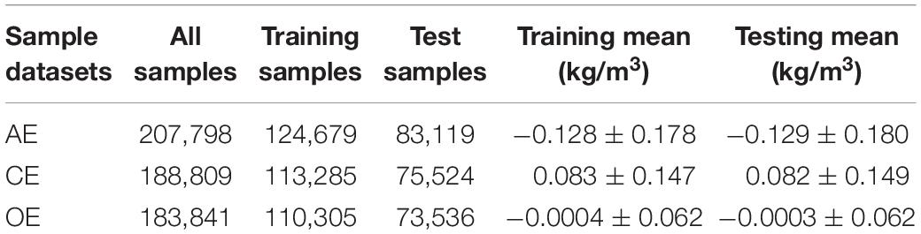
Table 1. Sample statistics of training and testing datasets.

Models

In this paper, a new hybrid model that combines the advantages of convolutional neural network (CNN) and extreme gradient boosting (XGBoost) is proposed. The proposed model is combined with two parts: feature extraction and classification. CNN is used to extract and select the features of the profile data at the bottom of the network, and the obtained high-dimensional feature vectors are inputted into the XGBoost model for profile classification. The experimental environment of model building is performed on a computer with an Intel i7-9700F CPU @3.00 GHz with 32 GB memory, Windows 10 OS, and Anaconda 3. Python is the main programming language, and CNN is implemented under the neural network framework Pytorch 1.5.1.

Convolutional Neural Network

A supervised CNN model is proposed to extract features from profiles. CNN model goes through a training process with inputted training profiles, and the cross-entropy loss is computed for back propagation to optimize the model parameters. The detailed process of the model is described as follows.

For our dataset with m profiles and k-dimensional vertical features, let $p_{train}^l=(d_{20},d_{21},d_{22},\mathrm{\dots },d_{k-1},d_k,k=1,000)$ be an input vector of the CNN, where d_z represents the PDA at the depth of z (m). The features extracted by the first hidden layer can be described as Equation (1).

$$Z_1=W_1\otimes P_{train}^l+b_1(1)$$

where ⊗ represents the convolution process. W₁ and b₁ are the weight and bias of the first hidden layer, respectively, and Z₁ is the output of the first hidden layer.

Then, other hidden layers can be described as Equation (2).

$$Z_i=W_i\otimes Z_{i-1}+b_{i-1},i=2,\mathrm{\dots },n(2)$$

where n is the number of the hidden layer. Suppose q(f₁,f₂,,f_j,,j = 64) = C(p^l) is the obtained feature vector from CNN, the process of XGBoost model can be defined as P = X(q,features_vertical), where P represents the output probability of XGBoost model, which is computed by softmax function. features_vertical represents the additional vertical structure features (see details in CNN-XGBoost Model). Therefore, the proposed model can be defined as Equation (3).

$$P=X\left[C(p_{train}^l)\right](3)$$

The cross-entropy loss is defined as Equation (4).

$$L=-\sum _{a=1}^c{y}_a\log P_a(4)$$

where y_a is the real label, P_a is the probability of class a, and c is the class number. The training process finished when the loss convergence. Then, the testing dataset $[p^l{}_{test}=(d_{20},d_{21},d_{22},\mathrm{\dots },d_{k-1},d_k,k=1,000)]$ are inputted into the model to evaluate accuracy.

Extreme Gradient Boosting

XGBoost is a highly effective scalable machine learning model developed by Chen and Guestrin (2016), which has been widely used in many fields to achieve state-of-the-art results on data challenges. It is greatly improved and optimized on the traditional Gradient Boosting Decision Tree, mainly including using the second-order Taylor expansion and introducing the regular term to prevent overfitting, which greatly promotes the accuracy, efficiency, and flexibility of the model. After the training of CNN model, a 64-dimensional feature vector is obtained and inputted into the XGB model. The principle of the XGBoost model is described as follows. For a dataset with n samples and m features D = {(x_i,y_i)}(|D| = n,x_i ∈ ℝ^m,y_i ∈ ℝⁿ), ${\widehat{y}}_i^k$ is the predicted result of x_i in round k. A tree boosting model output ${\widehat{y}}_i^k$ with K trees is defined as follows:

$$\widehat{y_i}=\sum _{k=1}^K{f}_k\left(x_i\right),f_k\in F(5)$$

where F = {f(x) = w_q(x)}(q:ℝ^m→T,w ∈ ℝ^T) is the space of regression or classification trees, w is the weight of the leaf child nodes of the regression tree, and q is the structure of the regression tree. T is the number of leaf nodes. In order to learn the parameters of this model, it is necessary to minimize the objective function:

$$Obj=\sum _{i}l(\widehat{y_i},y_i)+\sum _k\mathrm{\Omega }(f_k)(6)$$

where l in Equation (6) is a training loss function that measures the distance between the prediction $\widehat{y_i}$ and the object y_i. The second term in Equation (6) is defined as follows, which represents the penalty term of the tree model complexity.

$$\mathrm{\Omega }\left(f_t\right)=\mathrm{\gamma }T+\frac{1}{2}\mathrm{\lambda }\sum _{j=1}^T{\mathrm{\omega }}_j^2(7)$$

where γ is the regularization term (based on the number of leaves of the tree and the scores of each leaf), and T is the number of leaves. λ is the L2 regularization parameter, and the final prediction by summing up the score in the corresponding leaves is given by ω. XGBoost is a forward step-by-step algorithm, that is, in the round t iteration, adding a new model f_t needs to minimize the following target function:

$$Ob{j}^{(t)}=\sum _{i=1}^{n}l(y_i,{\widehat{y_i}}^{(t-1)}+f_t(x_i))+\mathrm{\Omega }(f_t)(8)$$

XGBoost algorithm uses second-order Taylor expansion for optimization. After the second-order Taylor expansion, the following formula is obtained:

$$Ob{j}^{(t)}=\sum _{i=1}^n\left[l(y_i,{\widehat{y}}_i^{(t-1)})+g_i{f}_t\left(x_i\right)+\frac{1}{2}{h}_i{f}_t^2\left(x_i\right)\right]+\mathrm{\Omega }\left(f_t\right)(9)$$

Denote I_j = {i|q(x_i) = j} as the instance set of leaf. Where $g_i={\partial }_{{\widehat{y}}^{\left(t-1\right)}}l(y_i,{\widehat{y}}^{\left(t-1\right)})$, $h_i={\partial }_{{\widehat{y}}^{\left(t-1\right)}}^{2}l(y_i,{\widehat{y}}^{\left(t-1\right)})$ are first- and second-order gradient statistics on the loss function. After substituting g_i, h_i, and into Equation (9), the formula can be rewritten as:

$$Ob{j}^{(t)}=\sum _{j=1}^T\left[G_j{w}_j+\frac{1}{2}\left(H_j+\mathrm{\lambda }\right)w_j^2\right]+\mathrm{\gamma }T(10)$$

where G_j = ∑_{i ∈ Ij}g_i, H_j = ∑_{i ∈ Ij}h_i. For a regression tree with a specific structure, the solution weight $w_j^{*}=\frac{G_j}{H_j+\mathrm{\lambda }}$ is used to evaluate the quality of the tree structure by deriving w_j. A greedy algorithm is used to determine the tree structure that starts from a single leaf and iteratively adds branches to grow the tree structure. Whether adding a split to the existing tree structure can be decided by the following function:

$$O_{split}=\frac{1}{2}\left[\frac{G_L^2}{H_L+\mathrm{\lambda }}+\frac{G_R^2}{H_R+\mathrm{\lambda }}-\frac{G^2}{H+\mathrm{\lambda }}\right]-\mathrm{\gamma }(11)$$

where I_L and I_R are the instance sets of the left and right nodes after the split and I = I_L∪I_R.

CNN-XGBoost Model

In this paper, the specific structure CNN-XGBoost model is used for eddy identification. Figure 2 visualizes the architecture of the model. We use six CNN building blocks with convolutional, batch normalization, activation layers, and a pooling layer. Because of the strong feature expression ability of CNN, the accuracy of the model will decrease with the increase in convolution layer, but restricting the depth of the model may reduce the classification accuracy. Therefore, we adopt a doubleconvpool structure. Doubleconvpool structure includes two convolution layers, two batch normalization layers, and one pooling layer. That is, there is no pooling layer between two consecutive convolution layers to realize the retention and transmission of feature information and balance between the high-dimensional characteristics of profile and model depth. Meanwhile, the model uses batch normalization and dropout to avoid overfitting. Then, the ReLU activation function is set after convolution to add nonlinear factors to increase the expression ability of the model. Each profile is inputted into the model as a one-dimensional feature vector (the depth range is 20–1,000 m). After six layers of CNN learning, a 64-dimensional feature vector is obtained and input into the XGB model. For the XGBoost classifier, in addition to the profile feature vector learned through the CNN model, the input features also include the spatiotemporal features of the eddy (location: longitude and latitude, month in which the eddy is recognized) as well as the vertical structure characteristics of eddy (including profile minimum, maximum and its corresponding depth, integral area of the entire profile, integral areas of 300 m interval, extreme values of 300 m intervals, and the corresponding depth) to comprehensively evaluate the characteristics of the eddy profile. After training and verifying the XGBoost model, the outputs are the probabilities of the classes “AE,” “CE,” or “non-eddy.”

FIGURE 2

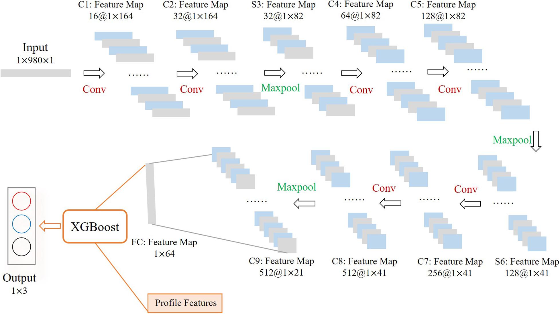
Figure 2. Convolutional neural network with extreme gradient boosting (CNN-XGBoost) architecture.

Results

Global Eddy Vertical Structure Characteristics

The vertical PDA profiles of Alt eddy are shown in Figure 3. The thick lines in Figure 3A represent the global average profiles over the entire time series. The thin lines are two randomly selected profiles in Alt eddy without smoothing. They show notable eddy vertical structures and accompanied by large noise and burr signal. Meanwhile, there is a dual-core in the AE (thin red line in Figure 3A). Even if the anomaly caused by the lower eddy core is smaller, the main eddy core should be located here with a wider eddy core. For CE (thin blue line in Figure 3A), obviously, in addition to a small anomaly in the sea surface, this eddy presents a single core structure with a depth ranging from about 50 m to nearly 400 m. The seasonal mean profiles from 2002 to 2019 are shown in Figure 3B, suggesting that the position and intensity of the eddy core will change along with the change in seasons, which is a reason that we add months as a feature to the model. Figures 3C,D present the latitude average vertical structure of the eddy PDA to show the variation in the depth and intensity of the eddy core on the latitude zone. On the whole, the eddy intensity in the northern hemisphere is stronger than that in the southern hemisphere, and the intensity of AE is stronger than that of CE. Along with the increase in latitude, the depth of the eddy core gradually increases, and a dual-core structure may appear in mid-latitude regions. Regarding the eddy intensity, we take about 200 m as the boundary. With the increase in latitude, the PDA intensity above 200 m becomes weaker and below 200 m becomes stronger. From the latitude-averaging profiles, we can see the general change trend of the eddy core, but for different small areas, the pattern of the eddy profiles will be greatly different (see Figure 6 for details). Thus, it is essential to consider the location (longitude and latitude of the eddy) when determining whether a float is located inside the eddy.

FIGURE 3

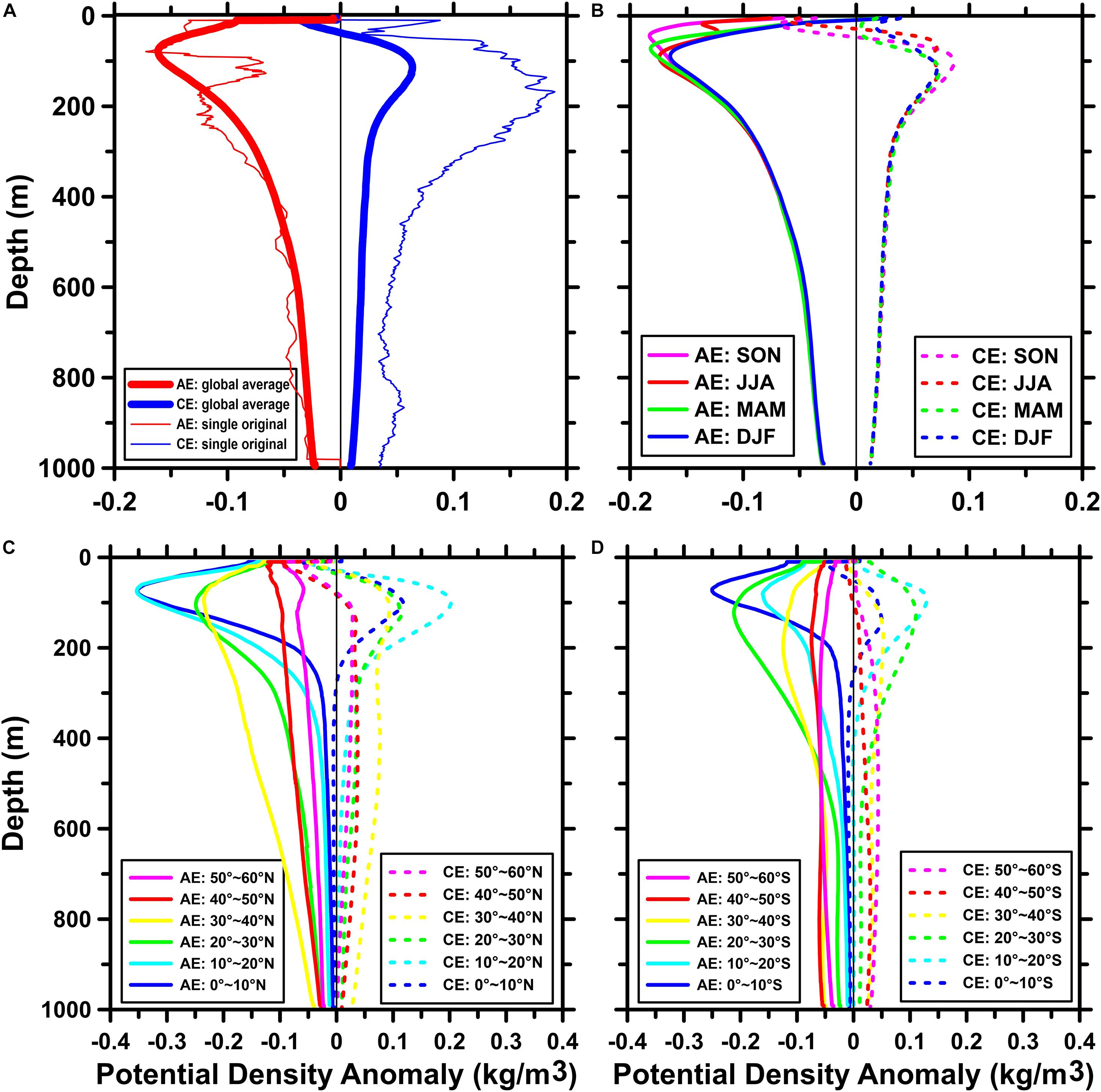
Figure 3. Vertical profiles of the potential density anomaly of Alt eddy. (A) Global average profiles from 2002 to 2019 (thick lines). The thin red (blue) line is the original eddy profile inside Alt anticyclonic eddies (AE) [cyclonic eddies (CE)], and the buoy number is 1901621 on March 26, 2018 and 1901817 on October 9, 2018, respectively. (B) Global average profiles in different seasons. (C) Latitudinal average profiles in the Northern hemisphere and (D) latitudinal average profiles in the Southern hemisphere.

Model Training Process

In order to reveal the effectiveness of the CNN-XGB hybrid model, we test the accuracy of CNN model, XGB model, and the hybrid model for profile classification. The input feature of CNN and XGBoost model is the PDA profile vector, and softmax is used as the classifier. The running time, accuracy, and sensitivity assessment of these three models are summarized in Table 2. Note that the sensitivity assessment refers to the proportion of a kind of eddies that are mistakenly classified into the other two types (i.e., AE is misjudged as CE or OE), so as to evaluate the specificity of the proposed algorithm to eddies in different polarity. It can clearly reflect that the classification accuracy of CNN-XGBoost model is better than that of CNN or XGBoost alone, and the accuracy can be improved by ∼4 and ∼6% on CNN and XGBoost model, respectively. The specificity analysis of the three models shows that the probability of AE being misjudged is less than that of CE. The reason for this result is that compared with the PDA induced by AE, CE is weaker (see Table 1 and Figure 3 for the mean PDA values and profiles of AE and CE, respectively). This result is also consistent with the conclusion that the proportion of abnormal CE is larger (see Chen et al., 2020 for details). In addition, AE (CE) is more likely to be judged as OE than CE (AE). It is comprehensible that eddies with weak signals are easier to be judged as OE (for its critical PDA signal close to zero) rather than the classification of the opposite polarity.

TABLE 2

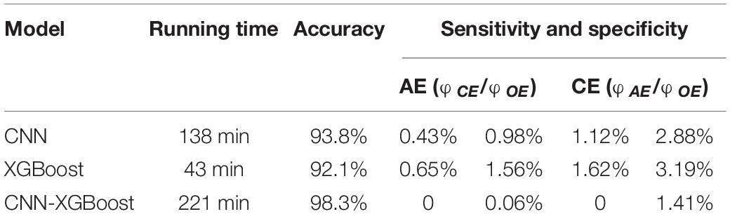
Table 2. Comparison of three different models.

To train CNN-XGBoost model, the first is the training of the CNN model. We used cross-entropy as the loss function, and the optimization algorithm of the training process adopts Adam algorithm. A 3 × 3 convolution kernel size is used in every convolutional layer, and the stride is 5. Furthermore, maximum pooling using a kernel of size 2 × 2 is added to prevent overfitting. We choose different learning rates (0.0005, 0.001, 0.003, 0.005, and 0.01) to experiment on the dataset. It shows that when the learning rate is 0.0005, the convergence speed is the fastest, and the loss function is the smallest when it converges, so this experiment uses 0.0005 as the value of the learning rate. After 100 epochs of training, the test accuracy of the CNN model can achieve ∼94%. Figure 4 presents the accuracy and loss variation on validation sets, showing that the loss and accuracy of the model have been well converged.

FIGURE 4

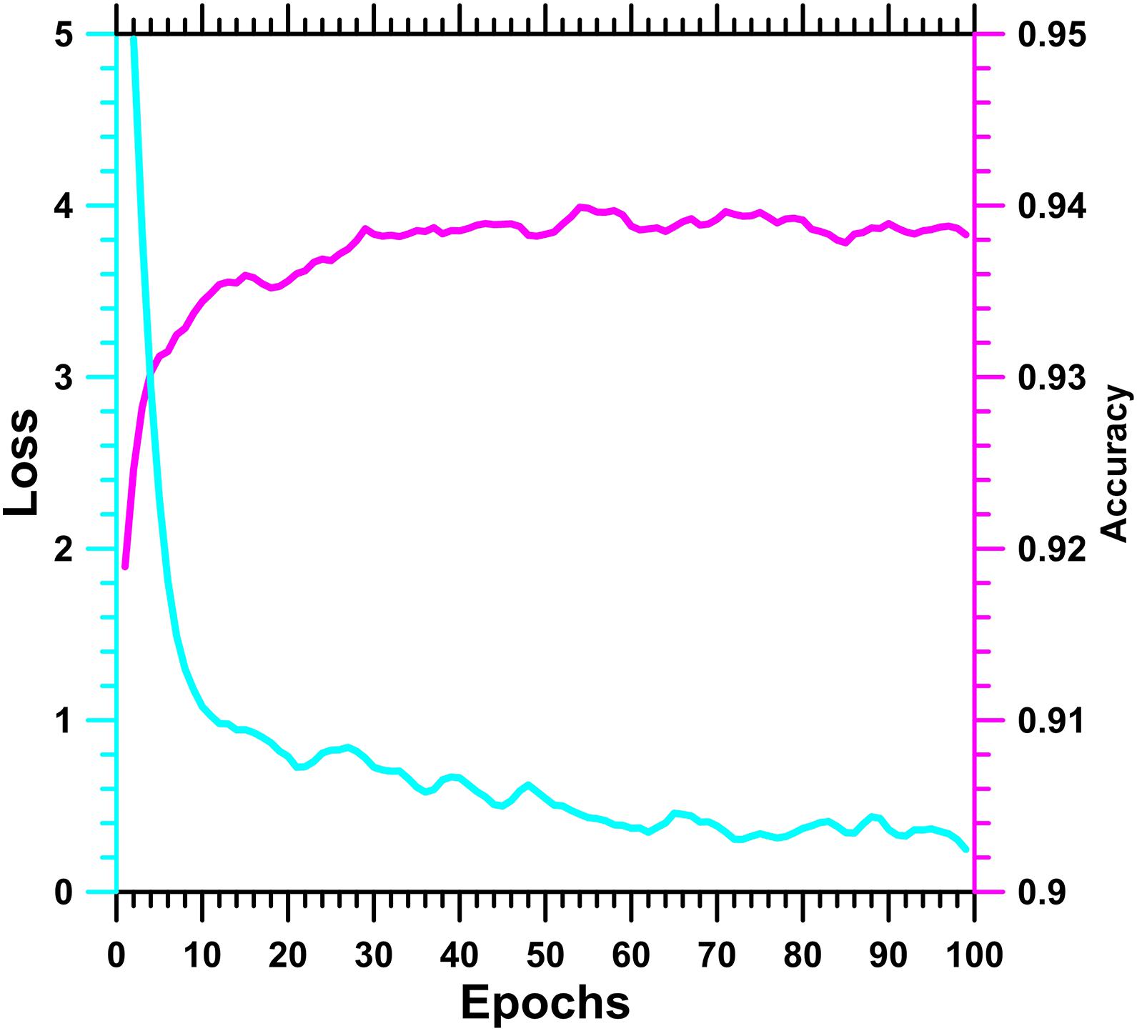
Figure 4. Accuracy and loss variation on validation sets of convolutional neural network (CNN) model.

For the XGBoost classifier, the Bayesian optimization is applied to obtain the best configuration of the hyperparameters. This optimization method is obtained from a Gaussian process prior and constantly updates the prior knowledge by considering the previous parameter information, whereas a conventional grid search or random search considers no prior parameter information. In addition, the Bayesian optimization process uses a small number of iterations and has a rapid running speed, allowing it to optimize algorithms with multiple parameters such as XGBoost. After parameters optimization, we select the best parameters including the eta, gamma, max_depth, and min_child_weight values of 0.4, 0.8, 10, and 1, respectively. The other parameters are set to the default values. The objective function is softmax for multiclassification, and the multiclass error rate is selected for the evaluation metric. After the 100 iterations’ training of XGBoost model, the CNN-XGB model accuracy reaches 98%.

Eddy Identification Based on CNN-XGBoost Model

The CNN-XGBoost model is used to learn and classify almost 120 million profiles that are not in the Alt eddy. It took only ∼17 min to classify the entire dataset, and then, we got the profiles that are outside Alt eddy but inside the eddy identified by the CNN-XGB method (CNN-XGB eddy). Recently, we proposed a methodology to effectively combine the vertical structure signals and sea surface topological structure of eddies based on a mathematical PDA algorithm (PDA eddy, Chen et al., 2020). Compared with this method, the CNN-XGB model has two significant advantages. First is higher computing efficiency. Based on the CNN-XGB method, we can scan the global profiles in < 20 min, while the mathematical method takes several days or even longer to complete the calculation, which reflects the unique advantages of AI model. Second is better spatial continuity. In order to take into account both the regional characteristics of eddy vertical structure and the number of training samples, we use 5° grid as the unit for eddy identification in the PDA algorithm, which limits the resolution of the algorithm to 5°. However, The AI model is not limited by the spatial grid and thus has stronger spatial continuity. In this section, we compare eddy features identified by the CNN-XGB model with those captured by the altimeter and obtained based on mathematical PDA methods, so as to verify the effectiveness of our model algorithm.

Vertical Structure of CNN-XGB Eddy

We first examined the vertical signals of the obtained CNN-XGB eddies. Figure 5 reflects the global average vertical structures of Alt eddy (short dashed line), PDA eddy (long dashed line), and CNN-XGB eddy (solid line). By and large, the global mean CNN-XGB eddy profiles have very significant PDA signals, which are much stronger than those of the Alt eddy and are almost as strong as PDA eddy signals, implying that the eddy identification based on CNN-XGB model is effective and robust. We can find out in detail that for these profiles, the anomaly increases with depth from the sea surface, reaches its maximum at ∼90 m and decreases thereafter. Although they present a similar depth position of eddy core, the magnitude of eddy core intensity varies greatly. For Alt eddy, the magnitude of maximum anomaly is ∼−0.18 kg/m³ for AE and only ∼0.08 kg/m³ for CE, while a maximum anomaly inside CNN-XGB AE (CE) is ∼−0.33 kg/m³ (∼0.20 kg/m³) for centered at ∼72 m (∼93 m). The eddy core intensity of CNN-XGB eddy is almost equal to PDA eddy (∼−0.32 kg/m³ for PDA AE and ∼0.21 kg/m³ for PDA CE, respectively) and present a slightly shallower eddy core depth compared to PDA eddy, which may due to the fact that the CNN-XGB model can find more eddies in the equatorial region where eddy cores are shallower (see Figure 7). The anomaly intensity of CNN-XGB eddy is almost twice as strong as Alt eddy, while the eddy core depth is close to each other, proving that some of the Argo profiles that are not captured by the altimeter show typical eddy vertical structure signals, which can be successfully extracted by the CNN-XGB algorithm.

FIGURE 5

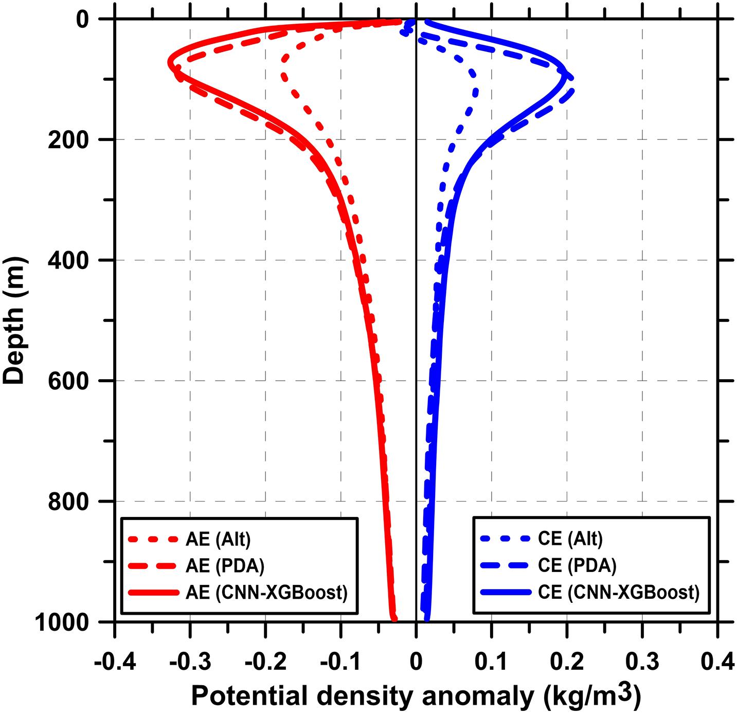
Figure 5. Global mean potential density anomaly profiles for different types of eddies from 2002 to 2019. The short dashed line is the profile of Alt-eddy. The long dashed line is the profile of potential density anomaly (PDA) eddy and the solid line is the vertical structure that is inside eddies through the convolutional neural network with extreme gradient boosting (CNN-XGBoost) model but not recognized by the altimeter. Red lines represent anticyclonic eddies (AE), and blue lines are cyclonic eddies (CE).

FIGURE 6

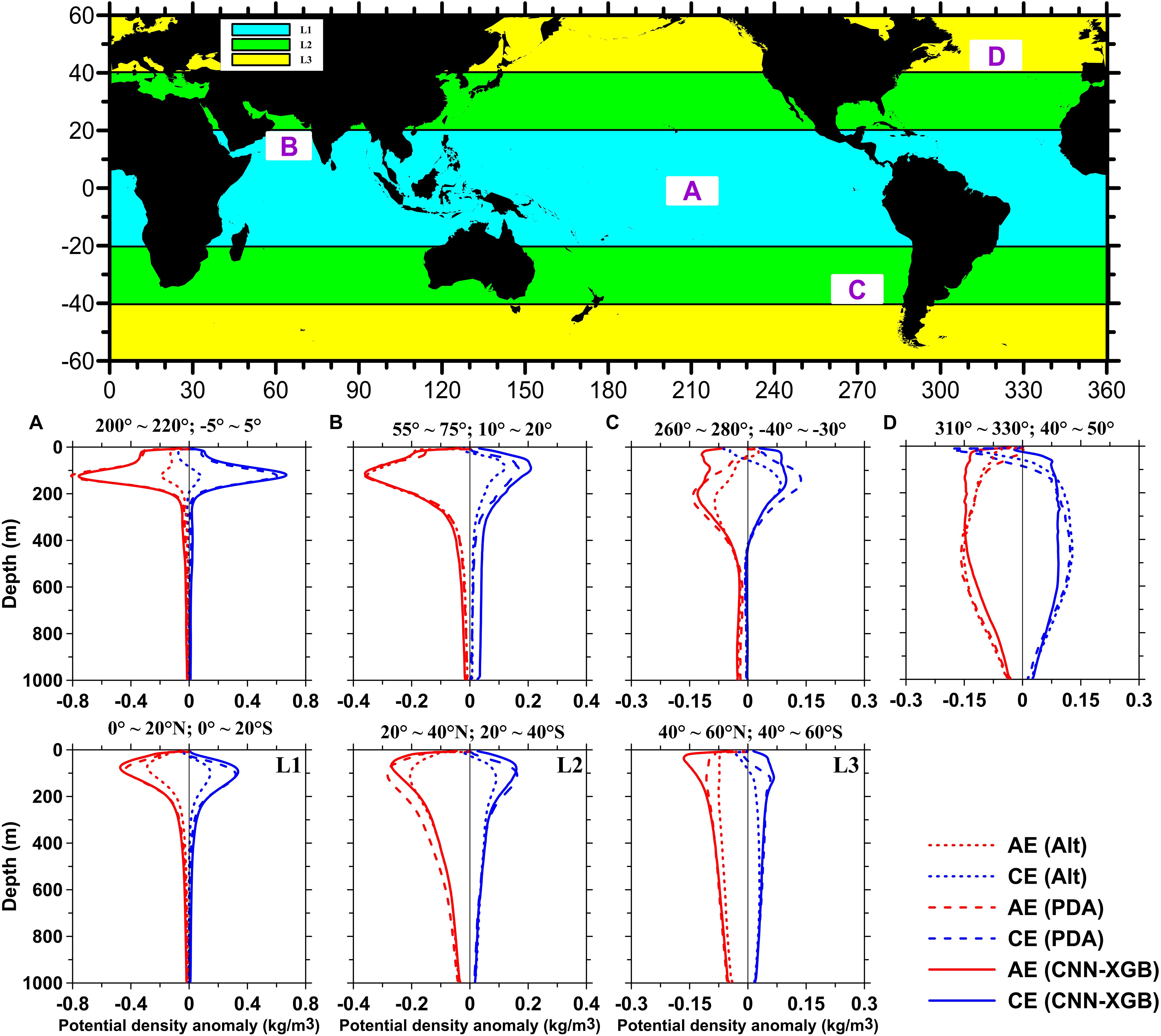
Figure 6. Mean potential density anomaly profiles of four areas in different latitude zones and average profiles of the different latitude zones. The white boxes marked with capital letters in the geographic distribution map represent the location of the corresponding areas, and the bands of different colors represent the corresponding latitude zones. (A,B) Average profiles in areas A and B in latitude 1 (L1: 0−20N and 0−20S), (C) Average profiles in area C in latitude 2 (L2: 20−40N and 20−40S), and (D) Average profiles in area D in latitude 3 (L3: 40−60N and 40−60S). The short dashed red (blue) lines are the profiles of Alt anticyclonic eddies (AE) [cyclonic eddies (CE)], long dashed red (blue) lines are the profiles of potential density anomaly (PDA) AE (CE), and the solid red (blue) lines are the profiles of CNN-XGB AE (CE).

FIGURE 7

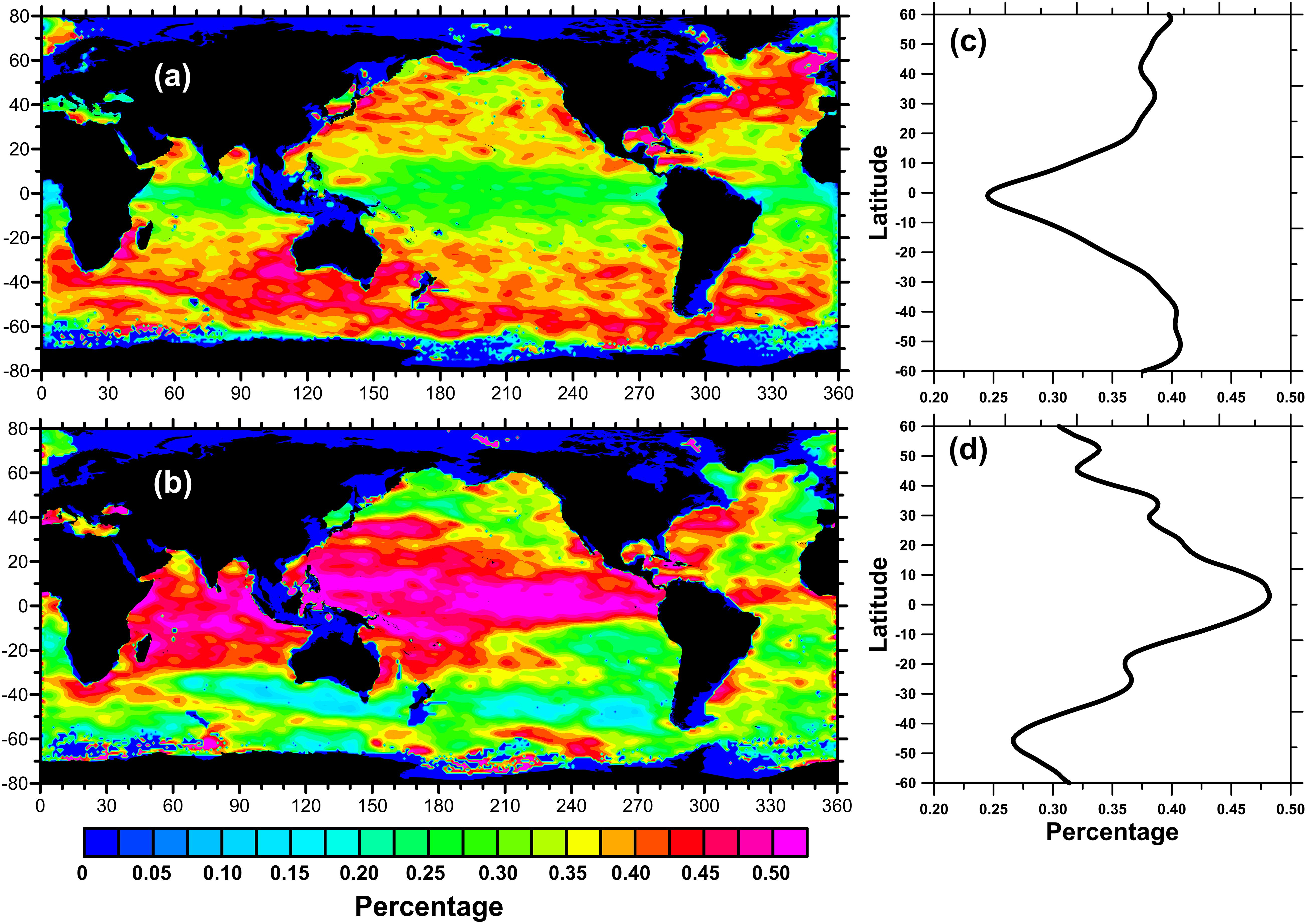
Figure 7. Global geographic distribution of profiles inside Alt eddy and convolutional neural network with extreme gradient boosting (CNN-XGBoost) eddy during 2002 to 2019 under a 1° grid. (a,b) The frequencies of Argo profiles in Alt eddy and CNN-XGBoost eddy occurrence with respect to all Argo profiles within the same grid, respectively. (c,d) Corresponding zonal distributions of Panels (a,b).

Since the vertical structure of eddies will have obvious inconsistencies with regional and latitudinal differences, we randomly selected four small areas in different latitude zones (white boxes in Figure 6) as well as the corresponding latitude zones (banded colors in Figure 6) to compare the vertical structures of the Alt eddy, PDA eddy, and CNN-XGB eddy to further verify the reliability of our results. Examining each panel, an overall impression is that CNN-XGB eddies show a stronger vertical signal than Alt eddies and a close signal with PDA eddies, which further proved that our eddy identification model is not only globally fitted but also regionally sensitive. The geographical distribution at the top of Figure 6 shows the location of the selected grid points and the division of latitude zone. Areas A and B are within the latitude range of 20N–20S (L1), which is covered by the light blue area. In area A, the signal at the eddy core (∼120 m) of CNN-XGB eddy is much stronger than that of Alt eddy, displaying a maximum of ∼−0.76 kg/m³ (∼−0.19 kg/m³) of CNN-XGB (Alt) AE and ∼0.66 kg/m³ (∼0.08 kg/m³) of CNN-XGB (Alt) CE. Area B locates in the Arabian Sea where the characteristics of the eddy core are consistent with Figure 7 in de Marez et al. (2019), showing that eddy-induced ocean anomalies in this area are mainly confined in the upper 300 m. The shift increases rapidly for both AE and CE, and the AE anomalies are slightly greater than those of CE. Looking at the mid-latitude, ranging from 20N–40N to 20S–40S (L2), which is covered by the green area, the eddy core goes deeper, and a double core structure may appear. A similar conclusion can be found in area C, which can be compared with the eddy structure in Pegliasco et al. (2015). Results show that the maximum PDA inside composite Alt CE is 0.08 kg/m³ at ∼170 m, while that inside the Alt AE is −0.09 kg/m³ at ∼240 m. In the CNN-XGB eddy profiles, a stronger PDA appears; the maximum inside the AE is ∼−0.13 kg/m³ and the maximum inside the CE is ∼0.1 kg/m³. A similar pattern is also found in the mean PDA profile of the latitudinal zone (L1–L3). Along with the increase in latitude, the magnitude of maximum anomaly remarkably decreases, but the signal of CNN-XGB eddy is always stronger than that of Alt eddy.

The vertical structure can intuitively reflect the strength of the eddy signal of the two identification methods. We suppose that such a large proportion of profiles with strong vertical structure signals are not recognized by the altimeter and may mainly include three aspects. First, a considerable part of CNN-XGB eddies is found distributed at the equator where the altimeter sampling interval is the largest (see Figure 7) so that even a part of eddies having notable sea surface characteristics is missing. Second, a part of the floats inside Alt eddy is relatively far away from the eddy center, which makes the vertical structure signal weaker because the vertical structure of the eddy weakens with the increase in the distance between the float and the eddy center. Third, even if the sea surface signal of the eddy is too small to be distinguished by the altimeter in higher latitude, it will have an evident vertical signal, and the existence of subsurface-intensified eddy that lacks strong surface signals cannot be eliminated.

Geographical Distribution of CNN-XGB Eddy

Another perspective to validate the effectiveness of eddy recognition is its global distribution characteristics. Figure 7 shows the global geographic distribution (left column) and the corresponding zonal distribution (right column) of Alt eddies and CNN-XGB eddies. In order to eliminate the influence of Argo floats location on the geographical distribution, the percentage of floats per 1° grid is calculated and shown. The percentage refers to the profiles falling into eddies divided by the total number of profiles in the corresponding grid. Comparing Figures 7a,b, the complementarity between the Alt eddy and CNN-XGB eddy is remarkable, showing that almost 50% of the profiles are inside eddies but are missed by the altimeter in the tropical ocean. The equatorial low latitude area is also the area where altimeter sampling is relatively sparse, and more eddies may not be detected. With the increase in latitude, the percentage of the profiles in Alt eddy increases gradually, while that in CNN-XGB eddy decreases. Since the geographic distance corresponding to the 1° spatial distance on the earth decreases with the increase in latitude, the spatial resolution of an altimeter with the same orbital spacing near the equator is much lower than that of high-latitude regions. The space distance of 1° latitude on the earth drops from about 111 km at the equator to about 55 km at the poles; that is, the corresponding geographic scale in the equatorial region is larger, and the spatial resolution of the altimeter is lower than that in the middle and high latitudes, so more eddies are missed. Through the vertical structure of the eddy, a large number of eddies in the equatorial region have been identified where the spatial resolution of the gridded altimetric products is not enough to capture the small-scale eddies. In addition, the geographical distribution of profiles inside CNN-XGB eddy has a consistency with that of the short-lived eddy proposed by Chen and Han (2019). It is also proved that eddy properties such as amplitude, vorticity, and kinetic energy are positively correlated with the eddy’s lifetime, and this can further confirm that there are plenty of eddies with a smaller radius and lower energy in the tropical equatorial region that can hardly be captured through the altimeter.

Further, both Alt eddies and CNN-XGB eddies are classified into AEs and CEs, as shown in Figure 8. Figures 8a,b are the difference between the Alt (CNN-XGB) AE and Alt (CNN-XGB) CE. Both of these two figures show a strip distribution of alternating positive and negative values, which further imply that our model has no eddy polarity preference. A belt of maximum in the tropical ocean also appears for both CNN-XGB AE and CE where altimeter eddy identification is known to be ineffective (Figures 8d,f). Figures 8c,d show the percentage of Alt (CNN-XGB) AE. It is obvious that in addition to picking up a large proportion of eddies in low latitudes, more missing AEs are found in AE accumulation areas such as the Kuroshio area, eastern Australia, and Southwest Atlantic. CE is the same, seeing in the South Pacific and North Atlantic for example (Figures 8e,f).

FIGURE 8

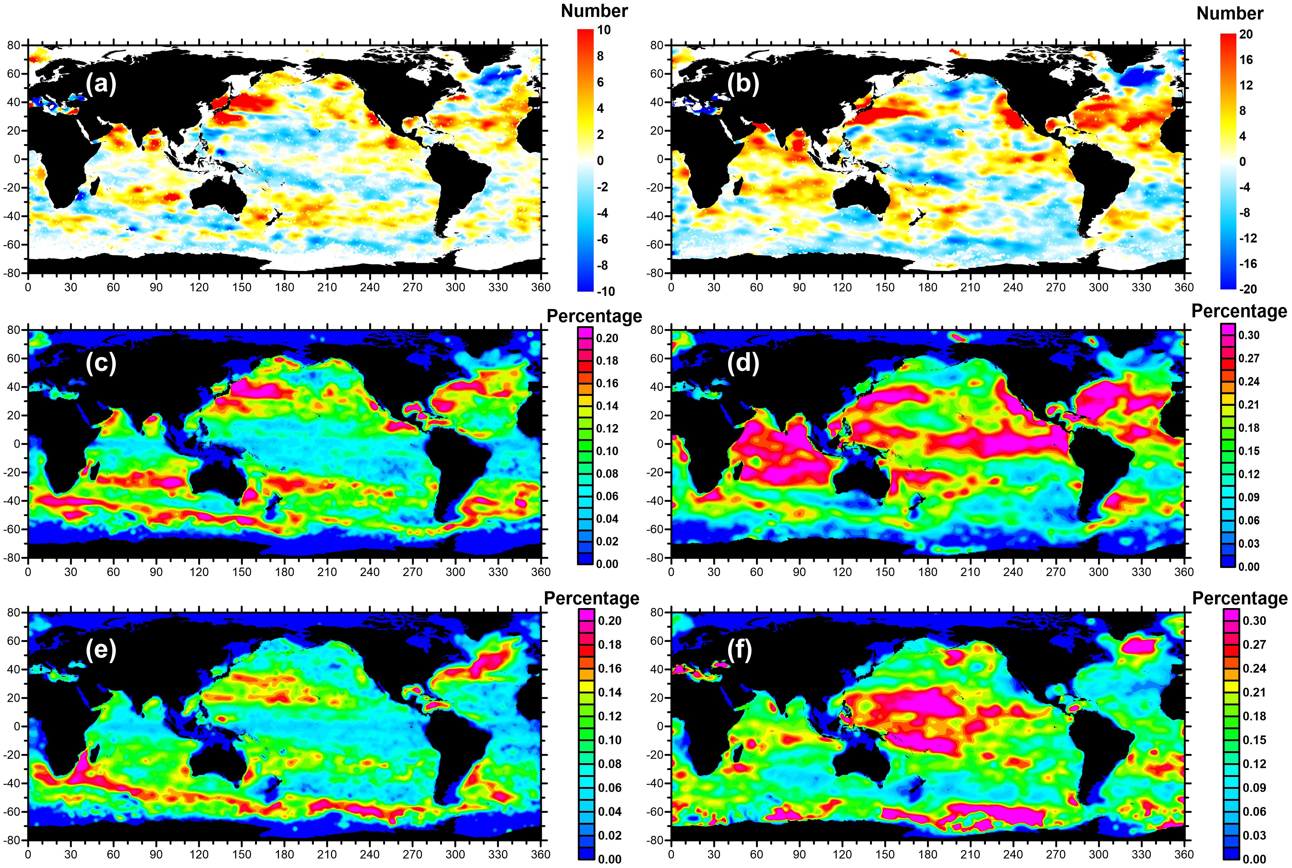
Figure 8. Global geographic distribution of Argo profile density per 1° × 1° grid during 2002 to 2019. (a) Distribution of numbers of Argos in Alt anticyclonic eddies (AE) minus the numbers of Argos in Alt cyclonic eddies (CE) in the corresponding grid. (b) Same as Panel (a) but is the Argos in CNN-XGB eddies. (c,d) The frequencies of Argo profiles in Alt AE and CNN-XGB AE occurrence with respect to all Argo profiles within the same grid, respectively. (e,f) same as Panels (c,d) but for CEs.

Table 3 summarizes the global average profile rate picked up by Alt eddy and CNN-XGB eddy. For the Alt eddy, the percentage of Argo captured is about 34.60%. After the CNN-XGB algorithm, the percentage of Argo inside eddy is increased by 36.04%, and the remaining 29.36% of Argo is indeed outside eddies. We further confirm the percentage inside CNN-XGB AE and CE for 18.69 and 17.35%, respectively, increases by ∼1% compared with Alt eddy.

TABLE 3

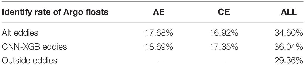
Table 3. Comparison of the statistics of Argo floats identified by altimeter and CNN-XGB.

Relationship Between Eddy Property and Its Vertical Structure

At present, we have realized the recognition of the eddy missed by the altimeter through artificial intelligence and the vertical structure of the eddy but only the recognition of the eddy point. It is well-known that an eddy is not only a vertical profile point but also a body with a certain radius and can cause the amplitude of the sea surface with a certain kinetic energy. Thus, the next step is to predict the surface characteristics of the eddy based on deep learning regression analysis, such as the radius, amplitude, and kinetic energy. Scatter diagrams of eddy radius, amplitude, and eddy kinetic energy (EKE) as a function of PDA intensity are illustrated in Figure 9. Basically, the three properties all have the most likelihood line in terms of data density, which displays a slowly increasing trend with PDA intensity: from ∼100 to ∼130 km for radius (Figure 9A), from ∼1 to ∼15 cm for amplitude (Figure 9B), and from ∼0 to ∼300 cm²/s² for EKE (Figure 9C). This result proves that there is an intrinsic correlation between the eddy surface properties and its vertical structure. It is feasible and reliable to invert the eddy surface parameters through the vertical structure characteristics.

FIGURE 9

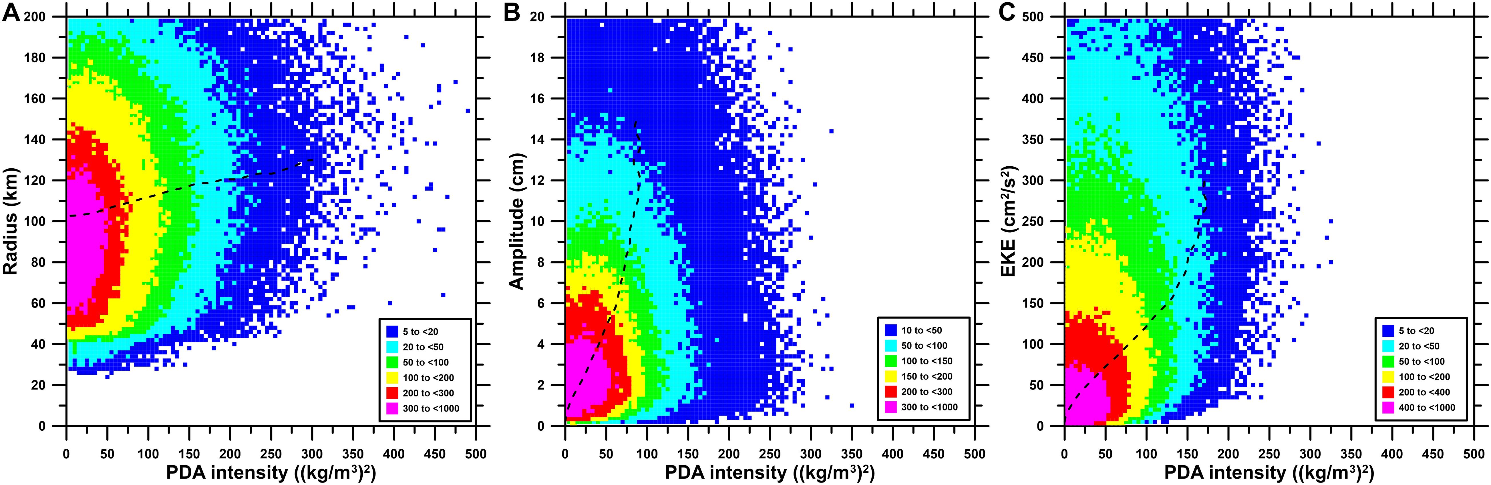
Figure 9. Scatter diagrams of eddy property versus potential density anomaly intensity during 2002–2019. (A) Radius, (B) amplitude, and (C) eddy kinetic energy (EKE). The color bars denote eddy numbers. The black dashed curves depict the most likelihood of eddy properties with respect to potential density anomaly intensity.

Conclusion

In this paper, a new hybrid model that combines the advantages of CNN and XGBoost is proposed to achieve oceanic eddy detection from 18-year Argo profiles. The major conclusions of the study can be summarized as follows.

First, the proposed CNN-XGBoost model has promising performance in extracting eddy vertical profile features. The CNN model has a design of six convolution layers, and a doubleconvpool structure is applied to improve the accuracy and efficiency of feature extraction. Moreover, the method can get the highest convergence when the learning rate is 5 × 10^–4. Furthermore, the 64-dimensional feature vectors learned from CNN are inputted into the XGBoost model combined with the profile position, date, and profile features. After 100 iterations, the final model is obtained, with a classification accuracy of 98%. Compared with CNN or XGBoost, the accuracy is improved by 4 and 6%, respectively. We further measured the sensitivity of the proposed model by calculating the erroneous judgment of AE and CE. Results show that compared with AE, CE is more likely to be misjudged (1.41 versus 0.06%) since the abnormal signal caused by CE is smaller than that of AE. Nevertheless, the CNN-XGBoost model presents the lowest error percentage among the three models with the highest misclassification rate of <2% (see Table 2 for details). The results provide an insight that the proposed deep learning method can be used as an effective methodology for eddy identification.

Second, vertical profiles of CNN-XGB eddies show a remarkable consistency with that of the Alt eddies. After carrying out the global average, latitudinal average, and grid average, we found that these eddies’ mean vertical shapes are homologous, and the vertical anomaly signal of the CNN-XGB eddy is similar or even stronger than that of the Alt eddy. For the global average, the magnitude of the maximum anomaly of Alt eddy is ∼−0.18 kg/m³ for AE and only ∼0.08 kg/m³ for CE, while the anomaly intensity of the CNN-XGB eddy is almost twice as strong as that of the Alt eddy, indicating ∼−0.33 kg/m³ for AE and ∼0.20 kg/m³ for CE. The reason why such a large proportion of profiles with strong vertical structure signals are not recognized by the altimeter may due to the larger sampling interval of the altimeter at the equator, the farther distance between the float and eddy center, and the existence of subsurface eddies.

Third, among Argo profiles from 2002 to 2019, ∼34.6% of the profiles are captured by Alt eddies, and about 36% of the profiles (∼19% for AE and ∼17% for CE) are actually inside eddies but missed by the altimeter and captured through our eddy identification method; the other ∼29% profiles are indeed outside eddies. The geographical distribution of the profiles inside CNN-XGB eddies is complementary to that inside Alt eddies. A prominent eddy belt with more than 50% of the profiles inside the CNN-XGB eddies is found in the tropical ocean. There is also the area abundant in short-lived eddy, which further proved that weak and small eddy may be lost with a greater probability. Consequently, the vertical profile datasets can be extended to improve the identification ability of the altimeter.

The present research shows that there is a positive correlation between eddy properties (e.g., radius, amplitude, kinetic energy) and the abnormal strength of eddy’s vertical structure. Therefore, based on the deep learning method, the inversion of eddy properties from its vertical structure should be further studied, so as to establish a more complete Argo-eddy identification dataset. In the spirit of reproducibility, the Python code will be available at https://github.com/, and we will also share the training and testing data used for this work to encourage competing methods and, especially, other deep learning architectures.

Data Availability Statement

The data used to support the findings of this study are available as follows. The altimeter all-sat merged sea level anomaly datasets generated for eddy identification can be found in the Archiving, Validation, and Interpretation of Satellite Oceanographic (AVISO, https://www.aviso.altimetry.fr/index.php?id=3122). The eddy identification dataset can be obtained from http://coadc.out.edu.cn/tfl/ and http://data.casearth.cn/ (Data ID: XDA19090202). Argo profile data can be obtained from ftp://ftp.ifremer.fr/ifremer/argo/.

Author Contributions

XC performed methodology, software, validation, data curation, visualization, and writing of the original draft. GC contributed to conceptualization, investigation, writing review and editing, and supervision. LG performed the model framework construction. BH performed validation and investigation. CC performed validation and review. All authors contributed to the article and approved the submitted version.

Funding

This research was jointly supported by the National Natural Science Foundation of China (No. 42030406), Marine Science & Technology Fund of Shandong Province for Pilot National Laboratory for Marine Science and Technology (Qingdao) (No. 2018SDKJ0102), and ESA-NRSCC Scientific Cooperation Project on Earth Observation Science and Applications: Dragon 5 (No. 58393).

Conflict of Interest

The authors declare that the research was conducted in the absence of any commercial or financial relationships that could be construed as a potential conflict of interest.

References

Amores, A., Jordà, G., Arsouze, T., and Le Sommer, J. (2018). Up to what extent can we characterize ocean eddies using present-day gridded altimetric products? J. Geophys. Res. 123, 7220–7236. doi: 10.1029/2018JC014140

CrossRef Full Text | Google Scholar

Andrade, I., Hormazabal, S., and Combes, V. (2014). Intrathermocline eddies at the Juan Fernandez Archipelago, southeastern Pacific Ocean. Lat. Am. J. Aquat. Res. 42, 888–906. doi: 10.3856/vol42-issue4-fulltext-14

CrossRef Full Text | Google Scholar

Bryden, H. L., and Brady, E. C. (1989). Eddy momentum and heat fluxes and their effect on the circulation of the equatorial Pacific Ocean. J. Mar. Res. 47, 55–79. doi: 10.1357/002224089785076389

CrossRef Full Text | Google Scholar

Chaigneau, A., Texier, M. L., Eldin, G., Grados, C., and Pizarro, O. (2011). Vertical structure of mesoscale eddies in the eastern South Pacific Ocean: a composite analysis from altimetry and Argo profiling floats. J. Geophys. Res. 116:C11025. doi: 10.1029/2011JC007134

CrossRef Full Text | Google Scholar

Chelton, D. B., Gaube, P., Schlax, M. G., Early, J. J., and Samelson, R. M. (2011a). The influence of nonlinear mesoscale eddies on near-surface oceanic chlorophyll. Science 334, 328–332. doi: 10.1126/science.1208897

PubMed Abstract | CrossRef Full Text | Google Scholar

Chelton, D. B., Schlax, M. G., and Samelson, R. M. (2011b). Global observations of nonlinear mesoscale eddies. Prog. Oceanogr. 91, 167–216. doi: 10.1016/j.pocean.2011.01.002

CrossRef Full Text | Google Scholar

Chen, G., Chen, X., and Huang, B. (2020). Independent eddy identification with profiling Argo as calibrated by altimetry. J. Geophys. Res. 125:e2020JC016729. doi: 10.1029/2020JC016729

CrossRef Full Text | Google Scholar

Chen, G., and Han, G. (2019). Contrasting short-lived with long-lived mesoscale eddies in the global ocean. J. Geophys. Res. 124, 3149–3167.

Google Scholar

Chen, T., and Guestrin, C. (2016). “XGBoost: a scalable tree boosting system,” in Proceedings of the Acm Sigkdd International Conference on Knowledge Discovery & Data Mining, San Francisco, CA, 13–17.

Google Scholar

de Marez, C., L’Hégaret, P., Morvan, M., and Carton, X. (2019). On the 3D structure of eddies in the Arabian Sea. Deep Sea Res. Part I. 150:103057. doi: 10.1016/j.dsr.2019.06.003

CrossRef Full Text | Google Scholar

Dong, C., Lin, X., Liu, Y., Nencioli, F., Chao, Y., Guan, Y., et al. (2012). Three-dimensional oceanic eddy analysis in the Southern California Bight from a numerical product. J. Geophys. Res. Oceans 117:46218. doi: 10.1029/2011JC007354

CrossRef Full Text | Google Scholar

Du, Y., Song, W., He, Q., Huang, D., Liotta, A., and Su, C. (2018). Deep learning with multi-scale feature fusion in remote sensing for automatic oceanic eddy detection. Inf. Fusion 49, 89–99. doi: 10.1016/j.inffus.2018.09.006

CrossRef Full Text | Google Scholar

Dunn, J. R., and Ridgway, K. R. (2002). Mapping ocean properties in regions of complex topography. Deep Sea Res. Part I 49, 591–604. doi: 10.1016/S0967-0637(01)00069-3

CrossRef Full Text | Google Scholar

D’Alimonte, D. (2009). Detection of mesoscale eddy-related structures through iso-sst patterns. IEEE Geosci. Remote Sens. Lett. 6, 189–193. doi: 10.1109/lgrs.2008.2009550

CrossRef Full Text | Google Scholar

Faghmous, J. H., Frenger, I., Yao, Y., Warmka, R., Lindell, A., and Kumar, V. (2015). A daily global mesoscale ocean eddy dataset from satellite altimetry. Sci. Data 2:150028. doi: 10.1038/sdata.2015.28

PubMed Abstract | CrossRef Full Text | Google Scholar

Faghmous, J. H., Styles, L., Mithal, V., Boriah, S., Liess, S., Kumar, V., et al. (2012). “Eddyscan: a physically consistent ocean eddy monitoring application,” in Proceedings: 2012 Conference on Intelligent Data Understanding; CIDU 2012, eds K. Das, N. V. Chawla, and A. N. Srivastava (Piscataway, NJ: IEEE), 96–103. doi: 10.1109/cidu.2012.6382189

CrossRef Full Text | Google Scholar

Fu, L. L., Chelton, D. B., LeTraon, P. Y., and Morrow, R. (2010). Eddy dynamics from satellite altimetry. Oceanography 23, 14–25. doi: 10.5670/oceanog.2010.02

CrossRef Full Text | Google Scholar

Gonzalez-Silvera, A., Santamaria-del-Angel, E., Millán-Nuñez, R., and Manzo-Monroy, H. (2004). Satellite observations of mesoscale eddies in the Gulfs of Tehuantepec and Papagayo (Eastern Tropical Pacific). Deep Sea Res. Part II 51, 587–600. doi: 10.1016/J.DSR2.2004.05.019

CrossRef Full Text | Google Scholar

Gordon, A. L., Shroyer, E., and Murty, V. (2017). An intrathermocline eddy and a tropical cyclone in the Bay of Bengal. Sci. Rep. 7:46218.

Google Scholar

Jeronimo, G., and Gomez-Valdes, J. (2007). A subsurface warm-eddy off northern Baja California in July 2004. Geophys. Res. Lett. 34:L06610. doi: 10.1029/2006GL028851

CrossRef Full Text | Google Scholar

Le Vu, B., Stegner, A., and Arsouze, T. (2018). Angular momentum eddy detection and tracking algorithm (ameda) and its application to coastal eddy formation. J. Atmos. Ocean. Technol. 35, 739–762. doi: 10.1175/JTECH-D-17-0010.1

CrossRef Full Text | Google Scholar

Liu, Y., Chen, G., Sun, M., Liu, S., and Tian, F. (2016). A parallel SLA-based algorithm for global mesoscale eddy identification. J. Atmos. Ocean. Tech. 33, 2743–2754. doi: 10.1175/jtech-d-16-0033.1

CrossRef Full Text | Google Scholar

McDougall, T. J., Feistel, R., Millero, F. J., Jackett, D. R., Wright, D. G., Kin, B. A., et al. (2009). The International Thermodynamic Equation of Seawater 2010 (TEOS-10): Calculation and Use of Thermodynamic Properties. Global Ship-based Repeat Hydrography Manual, IOCCP Report No, 14. París: UNESCO.

Google Scholar

Pegliasco, C., Chaigneau, A., and Morrow, R. (2015). Main eddy vertical structures observed in the four major Eastern Boundary Upwelling Systems. J. Geophys. Res. Oceans 120, 6008–6033. doi: 10.1002/2015JC010950

CrossRef Full Text | Google Scholar

Ren, X., Guo, H., Li, S., Wang, S., and Li, J. (2017). “A novel image classification method with CNN-XGBoost model,” in Digital Forensics and Watermarking. IWDW 2017. Lecture Notes in Computer Science, Vol. 10431, eds C. Kraetzer, Y. Q. Shi, J. Dittmann, and H. Kim (Cham: Springer).

Google Scholar

Ridgway, K. R., Dunn, J. R., and Wilkin, J. L. (2002). Ocean interpolation by four-dimensional weighted least squares: application to the waters around Australasia. J. Atmos. Ocean. Technol. 19, 1357–1375. doi: 10.1175/1520-0426(2002)019<1357:oibfdw>2.0.co;2

CrossRef Full Text | Google Scholar

Roemmich, D., Johnson, G., Riser, S., Davis, R., Gilson, J., Owens, W., et al. (2009). The Argo program observing the global ocean with profiling floats. Oceanography 22, 34–43. doi: 10.5670/oceanog.2009.36

CrossRef Full Text | Google Scholar

Sun, M., Tian, F., Liu, Y., and Chen, G. (2017). An improved automatic algorithm for global eddy tracking using satellite altimeter data. Remote Sens. 9:206. doi: 10.3390/rs9030206

CrossRef Full Text | Google Scholar

Tian, F., Wu, D., Yuan, L., and Chen, G. (2020). Impacts of the efficiencies of identification and tracking algorithms on the statistical properties of global mesoscale eddies using merged altimeter. Int. J. Remote Sens. 41, 2835–2860. doi: 10.1080/01431161.2019.1694724

CrossRef Full Text | Google Scholar

Zhang, Z., Wang, W., and Qiu, B. (2014). Oceanic mass transport by mesoscale eddies. Science 345, 322–324. doi: 10.1126/science.1252418

PubMed Abstract | CrossRef Full Text | Google Scholar

Zhang, L., Zhang, L., and Du, B. (2016). Deep learning for remote sensing data: a technical tutorial on the state of the art. IEEE Geosci. Remote Sens. Mag. 4, 22–40. doi: 10.1109/MGRS.2016.2540798

CrossRef Full Text | Google Scholar