Predicting Cetacean Distributions in the Eastern North Atlantic to Support Marine Management

Correia, Ana M.; Sousa-Guedes, Diana; Gil, Ágatha; Valente, Raul; Rosso, Massimiliano; Sousa-Pinto, Isabel; Sillero, Neftalí; Pierce, Graham J.

doi:10.3389/fmars.2021.643569

ORIGINAL RESEARCH article

Front. Mar. Sci., 19 May 2021

Sec. Marine Megafauna

Volume 8 - 2021 | https://doi.org/10.3389/fmars.2021.643569

This article is part of the Research Topic Small Cetacean Conservation: Current Challenges and Opportunities View all 51 articles

Predicting Cetacean Distributions in the Eastern North Atlantic to Support Marine Management

$\r\nAna M. Correia,*$ Ana M. Correia^1,2*

Diana Sousa-Guedes³

Ágatha Gil^1,2,4

Raul Valente^1,2

Massimiliano Rosso^1,5

Isabel Sousa-Pinto^1,2

Neftalí Sillero³

Graham J. Pierce^6,7,8

¹Interdisciplinary Centre of Marine and Environmental Research (CIIMAR), Matosinhos, Portugal
²Department of Biology, Faculty of Sciences, University of Porto (FCUP), Porto, Portugal
³Centro de Investigação em Ciências Geo-Espaciais (CICGE), Faculty of Sciences, University of Porto (FCUP), Porto, Portugal
⁴Department of Biology and Environment, Centre for the Research and Technology of Agro-Environmental and Biological Sciences (CITAB), University of Tras-os-Montes and Alto Douro, Vila Real, Portugal
⁵International Center for Environmental Monitoring CIMA Research Foundation, Savona, Italy
⁶Instituto de Investigacións Mariñas (CSIC), Vigo, Spain
⁷Oceanlab, University of Aberdeen, Aberdeen, United Kingdom
⁸CESAM and Department of Biology, University of Aveiro, Aveiro, Portugal

Data on species occurrence at the scale of their distributional range and the determination of their habitat use requirements are essential to support conservation and define management plans that account for their habitat requirements. For wide-ranging species, such as cetaceans, especially considering that their marine habitats include offshore areas, collection of such data is challenging. In the absence of dedicated surveys, alternative methodologies are needed, such as the use of data collected from platforms of opportunity and modelling techniques to predict distribution in unsurveyed areas. Using 6 years of cetacean occurrence data collected along cargo ship routes between the Iberian Peninsula, northwestern African coasts and the Macaronesian islands, we developed ecological niche models to assess habitat preferences and predict suitable habitats of the eight most frequently sighted cetacean taxa in the area. Explanatory variables used for model fitting included topographic, oceanographic, detectability, geographic and seasonal features. To provide a robust habitat characterisation, along with predictions of habitat suitability, making best use of occurrence datasets, we applied two modelling techniques, GAM and Maxent, which offer complementary strengths. Coastal areas provide important habitats for common and bottlenose dophins, while other dolphin species (spotted and striped dolphins) have a more oceanic distribution. The predicted niches of Cuvier’s beaked whale and minke whales are mainly in the high seas at northern latitudes. Suitable habitats for sperm whales and pilot whales are mostly in southern areas in continental slope regions. For all the species, models indicated that areas around seamount features offer suitable habitats, likely of high relevance in oligotrophic offshore waters. As such, dedicated survey effort in such areas would facilitate development and implementation of appropriate management plans, which are currently lacking. Our models offer an important contribution to baseline knowledge of cetacean distribution at basin-scale in the region and could support the definition of priority areas, monitoring plans, and conservation measures, essential to comply with the requirements of the EU Marine Strategy Framework Directive.

Introduction

One of the main issues for cetacean conservation is related to managing data deficiency. Lack of data is often viewed, at least by policy-makers, as an absence of any cause for concern. This interpretation often leads to a failure to develop conservation plans, delays in the implementation of management actions and reduced funding for scientific investigation on species that potentially are in need of more research effort (Parsons, 2016). Consequently, cetacean conservation is hindered, given that over 35% of cetacean species are categorised as “data deficient” by the IUCN¹. This leads to questions such as, how can we address data gaps and provide useful data for decision-makers? How can we apply the precautionary principle when data are deficient? How can we obtain comprehensive data on wide-ranging species that travel long distances over areas with no physical barriers? How can we sample remote areas like open-ocean waters where long-term monitoring programs are financially and logistically challenging? Possible solutions include the use of observation platforms of opportunity (OPOs), coupled with remote sensing data and ecological niche modelling.

Recently, the use of OPOs to collect long-term data on cetacean occurrence has increased considerably (Tobeña et al., 2016; Alves et al., 2018b; Tepsich et al., 2020). Sampling protocols and techniques used in data processing and analysis have been refined. Data collected from OPOs are now frequently used to conduct ecological niche modelling in order to assess cetacean distribution and understand its relationship with habitat characteristics (e.g., Correia et al., 2015, 2019b; Breen et al., 2017; Redfern et al., 2017; Derville et al., 2018; Fernandez et al., 2018; Fiedler et al., 2018; García et al., 2018; Passadore et al., 2018; Barragán-Barrera et al., 2019; García-Barón et al., 2019; Valente et al., 2019). Results from such models have been successfully applied in the definition of monitoring plans, management strategies and creation of Marine Protected Areas (MPAs) (Passadore et al., 2018; García-Barón et al., 2019).

Presence-only and presence-background models, which can be constructed without survey effort data, may provide reliable information on cetacean occurrence ranges (Redfern et al., 2006; MacLeod et al., 2008a; Friedlaender et al., 2011; Thorne et al., 2012; do Amaral et al., 2015; Derville et al., 2018; Fiedler et al., 2018; Smith et al., 2020). These algorithms are often an appropriate option to map habitat suitability of highly mobile species, for which data, especially effort-based, are hard to obtain (Sillero, 2011; Smith et al., 2020). This is especially so for cetaceans, since, in addition to horizontal mobility, they spend only a small proportion of time at the sea surface. On the other hand, the use of presence-absence models with effort-based data provides better insights into species habitat characteristics as such models account for surveyed habitat and quantify absence, for example, by using pseudo-absence data representative of the surveyed habitat (Brotons et al., 2004; Redfern et al., 2006; MacLeod et al., 2008a; Tepsich et al., 2014; Derville et al., 2018; Fiedler et al., 2018) or by dividing the survey track into segments and calculating encounter rates for each.

In general, the most frequently used predictors in ecological niche modelling for cetaceans are static habitat variables (such as those describing topography), as they are easier to quantify (they usually only have to be measured once) and to use for management purposes (e.g., definition of MPAs). Moreover, at least broadly speaking, there are good reasons to suppose that variables such as depth, seabed slope and substrate type are relevant to cetacean habitat choice (e.g., Redfern et al., 2006; MacLeod et al., 2008a; Viddi et al., 2010). Nonetheless, oceanographic processes play a fundamental role in determining the distribution of cetaceans, not only through their effects on prey availability but also in relation to physiological limits (e.g., the thermal niche, MacLeod et al., 2008b; MacLeod, 2009; Lambert et al., 2011, 2014). Hence, a combination of static and dynamic variables should be considered when modelling cetacean distribution, as well as for management purposes (Tobeña et al., 2016; Breen et al., 2017).

Another fundamental consideration is the spatial and/or temporal scale(s) (and resolution) of each variable to be used in the modelling process. The scales chosen can strongly influence model results and application. The association of the animals with oceanographic features may be stronger with ephemeral, mesoscale, seasonal, and/or more permanent features (Mannocci et al., 2017). For example, sea temperature may be relevant to cetacean distribution at several scales. At larger scales (i.e., low spatial resolution) sea-surface temperature can be used to define the limits of the thermal niches of cetaceans and their prey at different life-cycle stages, and to reflect the locations of water masses and current systems. At smaller scales (i.e., high spatial resolution), sea-surface temperature data can be used to determine the occurrence of mesoscale oceanographic features which may be associated with prey aggregations. Therefore, multi-scale models and/or the testing of several scales are recommended (Fernandez et al., 2018). Overall, the best model approach and methodology must be selected given the data available, sampled area and the aims of the models (Guisan and Zimmermann, 2000; Redfern et al., 2006), taking into account the biology of the species.

In the eastern North Atlantic, within the area encompassing the Iberian and northwestern (NW) African coasts and the Macaronesia, 36 species of cetaceans have been recorded, with the eight most frequently sighted representing all of the main guilds of cetaceans: small dolphins (bottlenose dolphins Tursiops truncatus, common dolphins Delphinus delphis, striped dolphins Stenella coeruleoalba, and Atlantic spotted dolphins Stenella frontalis), large dolphins (pilot whale Globicephala sp.), beaked whales (Cuvier’s beaked whales Ziphius cavirostris), sperm whales (Physeter macrocephalus) and baleen whales (minke whales Balaenoptera acutorostrata) (Correia et al., 2020). This is an area with a wide latitudinal and longitudinal range, encompassing substantial habitat variability (Mason, 2009; Sala et al., 2013). The composition of cetacean community species profiles varies among sub-regions (Correia et al., 2020), but cetaceans move and migrate across the entire area (Alves et al., 2018a; Valente et al., 2019). Therefore, to fully understand the habitat requirements of cetacean species in this area, distribution patterns need to be analysed at the basin-scale. However, similarly to many other areas in the globe, there are few data on cetacean occurrence in oceanic (high seas) waters of the eastern North Atlantic (Hammond et al., 2013; Correia et al., 2015; Jungblut et al., 2017).

In this study, we aimed to relate habitat characteristics to the distribution of the eight most frequently sighted cetacean species within the eastern North Atlantic, by using ecological niche models, at basin-scale, with data collected between 2012 and 2017 from OPOs along long-distance routes (CETUS Project; Correia et al., 2019a). A description of the spatial and temporal distributions of all cetacean species sighted is presented in Correia et al. (2020). Here, we applied two different modelling techniques, thus benefitting from the strengths of each in a complementary approach: a presence/pseudo-absence approach accounting for sampling effort using Generalised additive models (GAMs) to analyse cetacean-habitat relationships, and a presence/background approach including a larger dataset (all presence points) using Maximum entropy models (Maxent) to forecast habitat suitability for the eight cetacean species over the entire study area.

Materials and Methods

Study Area

Cetacean occurrence data were collected within the CETUS Project, a cetacean monitoring program in the eastern North Atlantic, which has been running since 2012. Here we analysed data spanning from 2012 to 2017. Through a collaboration with TRANSINSULAR, a Portuguese company for maritime transport, cargo ships are used as OPOs to collect data along commercial routes between continental Portugal, the Macaronesian archipelagos and NW Africa. In general, three commercial routes were sampled: Continental Portugal to Madeira (2012–2017); Continental Portugal to Azores (2014–2017) and Continental Portugal to Canary Islands, Northwest Africa and Cape Verde (2015–2017). Campaigns occurred mostly in summer and early autumn months (July–October) with the remaining months (February, March, May, June, November, and December) being surveyed in only one of the years. There were no campaigns in January or April. For spatiotemporal details on the sampled transects, see Correia et al. (2020).

The eastern North Atlantic is a very diverse region in terms of the topographic and oceanographic environment, which includes both narrow and wide continental platforms, abyssal plains, steep slopes, numerous seamounts and canyons, four archipelagos (Azores, Madeira, Canaries, and Cape Verde), major currents (Portugal, Azores, Canary, and Mauritania currents) and frequent occurrence of mesoscale eddies (Mason, 2009; Supplementary File 1).

Collection of Occurrence Data

Every year, each ship receives a team of two marine mammal observers (MMOs) for cetacean surveys. MMOs follow the standard sampling protocol for visual monitoring along line-transect surveys, from sunrise to sunset (Hammond et al., 2013; Tepsich et al., 2014; Correia et al., 2015). The survey data are subsequently divided into “legs,” i.e., periods of continuous observation (by at least one observer), generally corresponding to a full day from sunrise to sunset. Each leg is divided into “transects,” with each transect corresponding to an uninterrupted on-effort period, during which observers are monitoring actively.

Monitoring is performed from the front of the vessel, focused on a field of view of 180° centred on the heading of the vessel. Observers usually stand in both wings of the navigation bridge (at a height of between 13.5 and 16 m above sea level, considering maximum draught and speed, and depending on the ship), occasionally monitoring from inside of the ship when weather is uncomfortable (i.e., strong winds or moderate rain) but still suitable for surveying. Each observer stands on one side of the vessel and the two observers switch position every 60 min (approximately) to avoid fatigue and possible biases associated with different detection capacities of the observers. Moreover, in turns, both observers take (staggered) 1 h breaks for meals and two optional rests of up to 40 min (one in the morning and another during the afternoon). Each MMO usually covers 90° (one half of the overall field of view); at mealtimes and resting periods, the lone MMO covers the entire 180° range from one of the sides. Observers scan for cetacean presence with the naked eye, performing occasional scans with binoculars (fitted with a compass and a distance scale with seven or eight reticules, 7 × 50 mm). Apart from the year 2012, in which the route of the ship was recorded in a Garmin GPS and positions, along with associated data, were recorded on paper forms, all the data are recorded using a tablet with an inbuilt GPS and running the application MyTracks², which registers date and time, speed and direction of the route. After a survey leg, the data are stored in the app, in the internal memory of the tablet, and subsequently uploaded to a laptop. Then, at the end of each trip (from one port to another), all data are sent to the team coordinator on land for posterior data processing and analysis. The registers for each leg are always kept in two devices (at least) to avoid loss of data.

Weather conditions are assessed at the beginning and end of each survey leg and every time there is a significant change in the conditions. The following variables are recorded: sea state (using the Douglas scale), wind speed (using the Beaufort scale), visibility and the occurrence of rain. Visibility is measured on a standard categorical scale used by the crew for navigation purposes, which ranges from 1 to 10 (with 1 being visibility less than 50 m, and 10 being visibility over 50,000 m, see Supplementary File 2 for further details) and is estimated based on the definition of the horizon line and reference points at a known range (e.g., ships with an AIS system). The presence of marine traffic, categorised as small and large vessels (less than and over 20 m in length, respectively) in the area, detected with or without binoculars, is registered at the beginning and end of each survey leg, every hour and at every sighting. For this purpose, a 360° field of view is covered, with the observers performing a 360° sweep (i.e., searching all around their monitoring position, and not just in front of the vessel). Marine traffic data were not used in the present analysis. Sampling effort stops when weather conditions are unfavourable for cetacean monitoring, i.e., Beaufort and/or Douglas values > 4, visibility < 1 km or 5 in the visibility scale, and/or heavy rain, and when the survey stand is unavailable (e.g., during safety drills, manoeuvres). Any data collected until effort resumes are considered opportunistic (off-effort).

Whenever a cetacean species is sighted, both observers gather on the side of the boat where the animals were spotted in order to collect data on the occurrence. This marks the end of an on-effort transect.

Identification is attempted to the species level, although the taxonomic level registered is always the level to which the MMOs are confident of their identification. For group size estimates, the observers provide the minimum, maximum and most likely (best estimate) number of individuals in a sighting. Moreover, whenever possible, information on the heading of the group and its behaviour toward the ship (i.e., approaching, indifferent or avoiding) is also collected. After registering the sighting and collecting the above-mentioned data, each MMO returns to his/her side of the vessel, and a new on-effort transect starts. Data on the occurrence of pelagic megafauna other than cetaceans are also collected along the transect. However, observers record only taxonomic information and number of individuals, without interrupting the on-effort track.

During off-effort periods, cetacean sightings are still recorded as opportunistic (i.e., off-effort sightings). The same methodology for data collection is followed as much as possible, considering limitations associated with off-effort periods (i.e., poor weather conditions, observation stand unavailable, registering of another sighting).

Cetacean occurrences are reported as corresponding to the ship’s position at the moment of the cetacean sighting. Locations were not corrected based on the angle and distance to the cetacean, due to the errors associated with varying heights of the observation platform (e.g., due to the amount of cargo carried) and also to the interference in functioning of the compasses in the binoculars caused by the iron of the ship.

Environmental Data Collection

For ecological niche modelling, in addition to weather conditions and spatiotemporal variables, we derived habitat variables (static and dynamic) from satellite data at several temporal and spatial scales (see Supplementary File 2). The environmental variables were selected on the basis of their reported influence on cetacean occurrence (e.g., Redfern et al., 2006, 2017; Azzellino et al., 2012; Tobeña et al., 2016; Breen et al., 2017). Seabed topographic features are related with upwelling systems, turbulence and aggregation of prey species. Remotely sensed chlorophyll-a constitutes an adequate proxy for productivity while sea-surface temperature is commonly used to identify upwelling systems and thermal fronts and, in the study area, it shows a marked gradient from northern colder to southern warmer waters (Mason, 2009; Robinson, 2010). Finally, sea-surface altimetry is influenced by oceanographic dynamism including current systems. Sea level anomalies are a good indicator of up- and downwellings caused by the influence of topographic features or mesoscale eddies (Robinson, 2010).

Seabed slope was derived from bathymetry data. For distance to seamounts, we delimited topographic features classified as seamounts, banks, hills, ridges and rises in GEBCO³. We used contour lines created every 50 m and defined a polygon from the outermost closed contour line around the geographic location of the top of the features. Then, we calculated the distance from the base of the seamounts and from the coastline (distance to coast) to the sightings. Both slope and distances were computed using ArcGIS 10.5.

Chlorophyll-a and sea-surface temperature were obtained from NASA⁴ and are ocean products derived from the satellite Aqua, through the sensor MODIS. The algorithms return the near-surface concentration of chlorophyll-a (from in situ remote sensing reflectance) and temperature (from measured radiances). We extracted both variables at two different spatial scales (4 and 9 km) and two different temporal scales (8-day and monthly).

For altimetry, the mean sea level anomalies were obtained from Ssalto/Duacs multimission altimeter products provided by AVISO⁵. The sea level anomalies are sea-surface heights computed with respect to a 20-year mean profile (1993–2012). We used delayed products⁵, available around 2 months after collection, after re-analysis and re-processing. For this variable, 8-day and monthly resolutions were computed by averaging daily products.

Ecological Niche Modelling

We used two ecological niche modelling techniques, recognising the strengths of each as reported in the literature (e.g., Derville et al., 2018; Fiedler et al., 2018). Each type of algorithms (GAM and Maxent) forecast different things: presence-absence algorithms such as GAM distinguish between occupied and non-occupied habitats, while presence-background algorithms such as Maxent distinguish between suitable and unsuitable habitats (Sillero, 2011). GAM is accounting for the sampling effort in the transect, as absences cannot be guaranteed, and modelling the observed distribution of the species at the moment of the survey. GAMs were used to analyse species-habitat relationships and explore species habitat preferences, including seasonality of dynamic variables and a time variable (day of the year). Only on-effort records of occurrence were used. On the other hand, Maxent models the habitat suitability of the species by comparing the species presences with the available habitat (i.e., background). These were used to model of the realised niche of the species and map habitat suitability across the entire study area. In this case, dynamic variables were time-averaged, as there were insufficient data to model monthly (or seasonal) cetacean distributions. Nevertheless, taking into account the complementary approach, seasonality was not lost in the analysis as it was already introduced and assessed with the GAM models. For Maxent, all occurrence records were included (on and off-effort), therefore allowing for the use of the entire set of presence points.

Explanatory variables were chosen to reflect spatiotemporal, detectability and environmental factors (Supplementary File 2). Previous work with CETUS dataset (Correia et al., 2019b) prove that it is important to include detectability factors (sea state, wind state and visibility) in the modelling process and the combination of detectability, spatiotemporal and environmental predictors has been previously applied (and recommended) for cetacean ecological niche models (e.g., Díaz Lopez and Methion, 2017, Díaz López and Methion, 2018; Correia et al., 2019b).

We fitted models for the eight most frequently sighted species with, at least, 30 presence records collected on-effort (Stockwell and Peterson, 2002): common dolphin, Atlantic spotted dolphin, striped dolphin, bottlenose dolphin, Cuvier’s beaked whale, pilot whale, sperm whale, and minke whale.

Generalised Additive Models (GAMs)

For GAMs, we chose a presence/pseudo-absence approach based on used/available habitat (Pearce and Boyce, 2006; Elith and Leathwick, 2009; Correia et al., 2015, 2019b), with used (cetacean occurrence) and available (survey route) habitat points combined to generate a binary (1,0) response variable. We fitted binomial GAMs (with link: logit) to these response variables, allowing a maximum of four splines (k = 4) to limit the complexity of smoothers describing the effects of explanatory variables. The set of available points was generated as in Correia et al. (2015, 2019b), by creating equidistant points (every 5 km) along all on-effort transects. This guarantees an appropriate number of pseudo-absences representative of the environmental space (Barbet-Massin et al., 2012; Virgili et al., 2017). Moreover, the survey effort is taken into account in the models as regions with more surveyed legs result in more points of available habitat than those regions surveyed less often (i.e., with fewer surveyed legs). As points of available habitat were created randomly along surveyed legs (5 km equidistant), we looked for potential spatial and temporal overlap between these points and the cetacean occurrence points, to delete any erroneous pseudo-absence points. In practice, none of the selected pseudo-absence points coincided with locations at which cetaceans were present. The values of the explanatory variables were obtained for the set of used and available points. To derive values for oceanographic variables, we used Marine Geospatial Ecology Tools (MGET) for ArcGIS (Roberts et al., 2010).

Prior to modelling, we computed Pearson correlations between all pairs of explanatory variables to allow us to exclude highly correlated variables from the same model, using a threshold of 0.75 (after Marubini et al., 2009). Distance to coast and depth were the only pair of variables which were highly correlated. Both were of interest, hence, we first fitted a GAM model with depth as the predictor and distance to coast as the response variable. The depth and the residuals of this model were then used as explanatory variables in subsequent models (see Smith et al., 2011). The resulting spline for the residuals term should be interpret as the effects of proximity to coast in the species occurrence, at a given depth. Moreover, we assessed multiple correlation among explanatory variables through the Variance Inflation Factor (VIF, with a threshold of 3) (Zuur et al., 2010). All VIF values were lower than the threshold, so no additional variables were removed.

Following Correia et al. (2015, 2019b), and to account for varying group sizes, we included the best estimate of the number of animals sighted in a group as a weight parameter in the models. For (pseudo-)absences, the weight was always 1, while the presences were weighted according to the group size associated with the sighting. For species usually seen singly or in small groups (sperm whales, Cuvier’s beaked whales and minke whales), the weight was equal to the number of animals sighted in the group (group size best estimate). For species usually sighted in large groups (common dolphins, spotted dolphins, striped dolphins, bottlenose dolphins, and pilot whales), there was a wide range of group size and high uncertainty on the best estimate. As such, for these species, we assigned weights as follows: 1–5 animals, weight = 1; 6–20 animals, weight = 2; > 20 animals, weight = 3.

We considered only main effects of the variables, and started with saturated models including all static variables, followed by backward selection (Qian, 2009; Correia et al., 2015, 2019b). In the resultant model from this process, we selected the “best” scale for each of the dynamic predictors based on forward selection. This was necessary to avoid including correlated variables in the model, since each of the oceanographic variables showed correlations between values associated with the different spatiotemporal resolutions. We then performed a final backward selection. We selected the best models by using the Akaike Information Criterion (AIC) as a measure of goodness of fit, choosing the model with the lowest AIC value at each step of the model fitting process, i.e., comparing otherwise identical models with or without a specific explanatory variable. If the difference in AIC values between two models was less than 2, the models were compared using a Chi-squared test (Zuur et al., 2007). Whenever differences between AIC values were not statistically significant (based on δAIC < 2 and the chi-squared test result), we kept the simplest model in the backward selection process (following the principle of parsimony, e.g., Burnham and Anderson, 2002), or the highest resolution for the oceanographic variables (4 km over 9 km for spatial resolution, and 8-day over monthly for temporal resolution). If a spline was close to linear (with estimated degrees of freedom of ∼1), we removed the smooth term and fitted a linear function. We also checked final models for influential data points [all Hat values were under 0.25, indicating no strongly influential data points; the usual cut-off is 1.0 (Zuur et al., 2007)] and for relationships between residuals and explanatory variables (no clear patterns were seen). Finally, we evaluated the models by creating two random subsets of data: fitting and evaluating sets (75 and 25% of the data, respectively). The prediction power of the models was determined using the Area Under the Curve (AUC) of the Receiving Operator Characteristic (ROC) plot (Beck and Shultz, 1986; Liu et al., 2005). Random models have an AUC equal to 0.5; the closer an AUC is to 1, the higher discriminatory power of the model.

Models were developed using the “mgcv” package in R 3.4.4. (R Core Team, 2018) with R Studio.

Maximum Entropy Models (Maxent)

We modelled the ecological realised niches (see Sillero, 2011) of the eight species using the Maximum Entropy method implemented in Maxent 3.4.1. software⁶ (Phillips et al., 2006, 2017), a correlative niche algorithm for presence-only and background records (Guillera-Arroita et al., 2014). This method distinguishes between suitable and unsuitable habitats (Sillero, 2011). Maxent starts with a uniform probability distribution (gain = 0) and alters one weight at a time to maximise the likelihood of the occurrence data set, converging to the optimum probable distribution (Phillips et al., 2006, 2017). The output values range from 0.0 to 1.0, representing the habitat suitability (not the occurrence probability, as presence-absence algorithms do; Sillero, 2011).

Maxent generates a background sample of points, randomly selected from the whole study area, without any reference to the presence or absence of the species (Phillips et al., 2009; Elith et al., 2011; Guillera-Arroita et al., 2014). Thus, the background sample of points provides a spectrum of the available conditions, not meaning that species are absent (Phillips et al., 2009). Model performance improves if background points are extracted from areas near to species presences (Phillips et al., 2009). For this reason, we clipped the environmental variables with four different buffer sizes (5, 10, 20, and 50 km) around the cetacean presence points, selecting the random background points from within the buffer area. We then projected the models onto the whole study area. We defined the buffer sizes considering visibility (height of the observation deck, visibility range) during at-sea surveys and the likelihood of observers detecting different cetacean species (dolphins jumping or travelling vs. blow of the whales, etc.) (after Fourcade et al., 2014), as follows: up to 5 km, most animals are spotted under favourable conditions and jumping dolphins near the ship are sighted even in off-effort weather conditions; at a 10 km range, whales’ blows are seen and some jumping dolphins can still be spotted under favourable weather conditions; 20 km is the most common visibility range during CETUS surveys (with ships at a distance of ∼20 km still visible at the horizon line, as confirmed with the AIS system of the cargo vessel); the maximum visibility range ever recorded was 50 km (with ships being spotted at the horizon line at a distance of ∼50 km, range confirmed with the AIS system of the cargo vessel).

We selected five explanatory variables with between-variable Pearson correlations lower than 0.75 (Supplementary File 2): slope, chlorophyll-a, distance to seamounts, sea surface temperature, and depth. Distance to coast (correlated with depth) and latitude (correlated with sea surface temperature) were excluded. We did not include mean sea level anomaly due to its very low spatial resolution. We averaged the dynamic variables (chlorophyll-a and sea surface temperature) during the fieldwork period (Continental Portugal-Madeira: July–October 2012; June–October 2013; August–October 2014; June–October 2015; July–October 2016; September 2017; Continental Portugal-Azores: July–September 2014; July–October 2015; July–October 2016; July–October 2017; Continental Portugal-Canarias-Cabo Verde: May–October 2015; February-March and August–December 2016; June–September 2017) in Macaronesia region using 8-day resolution files with Raster Calculator in QGIS. The static variables remained the same for all periods. The spatial resolution of the environmental variables chosen was 4 km. We run Maxent with default settings, using 70% of the points as training data and 30% as test data. Duplicated records (i.e., two or more presences in the same pixel) were eliminated, thus we included only one presence per pixel. We built 100 model replicates for each species and gathered the arithmetic mean and the standard deviation for each set of 100 replicate models, as Maxent is a machine learning method. We ran Maxent in clog-log format (Phillips et al., 2017).

Model performance was evaluated based on the AUC of the ROC plot (Liu et al., 2005). In addition, as AUC is designed for presence-absence algorithms and not presence-only methods, we calculated a set of 100 null models for each species, following the methodology by Raes and ter Steege (2007). For this, we created 100 different datasets with the same number of random points as the species presences, following a Poisson distribution (suitable for counts, as in this case of number of presences). We obtained the AUC values of the ROC plots for each set of 100 null models. Then, we compared the training AUC values between species models and null models using a Kruskal-Wallis test. Null models were calculated in R 3.4.4. (R Core Team, 2018) using ‘dismo 1.1-4’ package (Hijmans et al., 2017).

The importance of each environmental variable was determined by the average percentage of contribution and permutation importance of each variable to the models through factor analysis: (1) a jack-knife analysis of the average AUC using training and test data; and (2) a calculation of the average percentage contribution of each variable to the models. For this purpose, the variables were excluded in turn and a model was created with the remaining variables; then a model was created using each individual variable.

Results

Sightings and Survey Effort

A total of 124,428 km of survey effort was distributed along three main routes, from continental Portugal to the Azores, to Madeira and to Cape Verde (the latter with stopovers in the Canary Islands and Northwest Africa) (Supplementary File 1). We collected 2807 sightings of which 1266 were analysed within this study, i.e., those of the eight most frequently sighted species (919 collected on-effort and 347 recorded opportunistically): D. delphis (394 sightings, of which 262 were on-effort), S. frontalis (226 sightings, 167 on-effort), S. coeruleoalba (154 sightings, 119 on-effort), T. truncatus (134 sightings, 92 on-effort), Z. cavirostris (64 sightings, 51 on-effort), Globicephala sp. (59 sightings, 44 on-effort), P. macrocephalus (152 sightings, 116 on-effort), and B. acutorostrata (92 sightings, 75 on-effort). Since 11 single sightings included two of the selected species (i.e., species were sighted in association with each other), those are accounted twice above when presenting the number of sightings by species (Supplementary File 1).

Ecological Niche Models

GAM and Maxent Models: Overview

All models performed better than a random model (AUC > 0.5). From the eight final GAM models, the best was that obtained for Globicephala sp., with an AUC of 0.93 and 26.8% of deviance explained, while the worst was that obtained for S. frontalis, with an AUC of 0.81 and 7.45% of deviance explained. All eight final models included variables related to detectability, spatiotemporal variables, and environmental (both static and dynamic) factors (Table 1). With the exception of S. frontalis, wind state affected the detectability of all species, with a general decrease of recorded occurrence with increased wind speed. S. frontalis occurrence was influenced by sea state, with an increase of detections up to sea state 2, and a roughly constant likelihood of detection thereafter. The detection of S. coeruleoalba, P. macrocephalus, and B. acutorostrata, increased with improved visibility (Figure 1).

TABLE 1

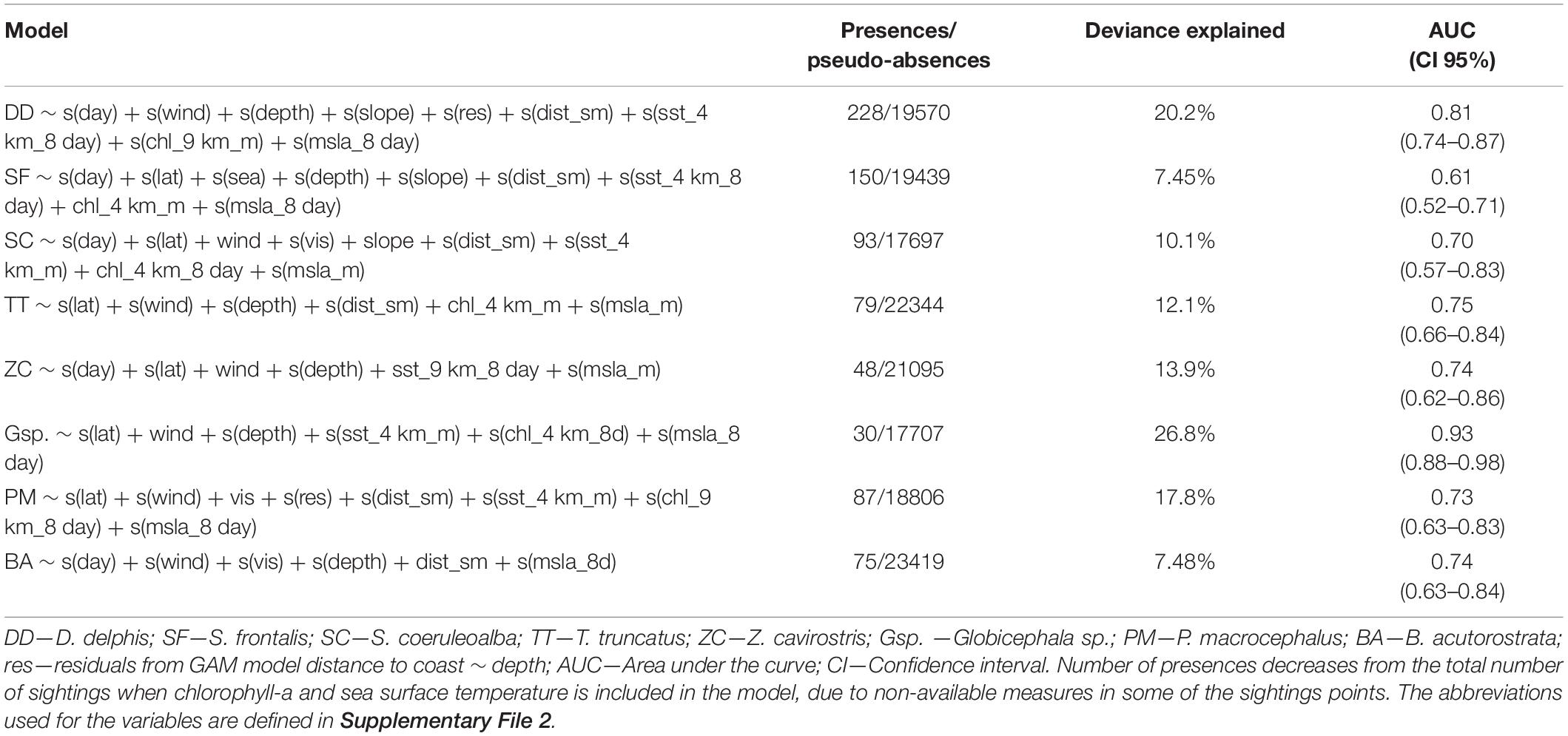
Table 1. Results from the best final GAM models developed for the eight most frequently sighted species.

FIGURE 1

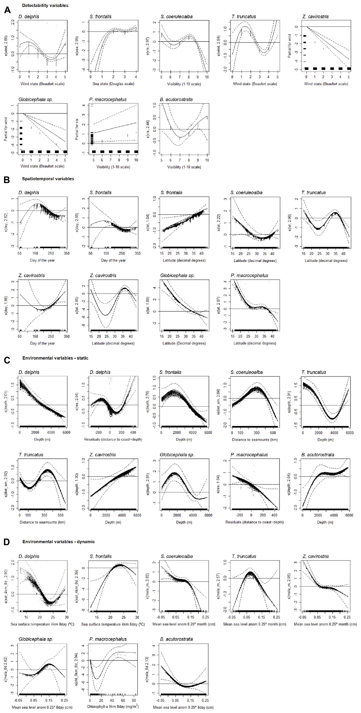
Figure 1. GAM fitted splines of the response variable species presence as a function of the explanatory variables for the environmental model produced for the eight most frequently sighted species. The degrees of freedom are shown in brackets on the y-axis. Tick marks above the x-axis indicate the distribution of observations. Dashed lines delimit the 95% confidence intervals of the spline functions and dots on the graph area represent the residuals. lat—latitude, wind—wind state in the Beaufort scale, dist_sm—distance to seamounts, chl—chlorophyll-a, msla—mean sea level anomalies. (A) Detectability variables; (B) spatiotemporal variables; (C) environmental static variables; (D) environmental dynamic variables.

The best Maxent models were obtained with a buffer size of 50 km (results are not shown for the other buffer sizes). The eight Maxent models had mean training AUC values close to 0.8 and test AUC close to 0.7. For all models, training AUC were significantly higher than those of null models (Kruskal-Wallis with p-values < 0.001). The best Maxent model was obtained for the most frequently sighted species (D. delphis), with a training AUC value of 0.85 and test AUC of 0.83, while the worst model was obtained for spotted dolphin (S. frontalis), with a training AUC of 0.75 and a test AUC of 0.69 (Table 2). The explanatory variable that contributed most to the B. acutorostrata and Z. cavirostris Maxent models was distance to seamounts. For D. delphis, Globicephala sp., and T. truncatus models, the most important variable was depth; for P. macrocephalus, S. coeruleoalba, and S. frontalis it was sea surface temperature (Table 2).

TABLE 2

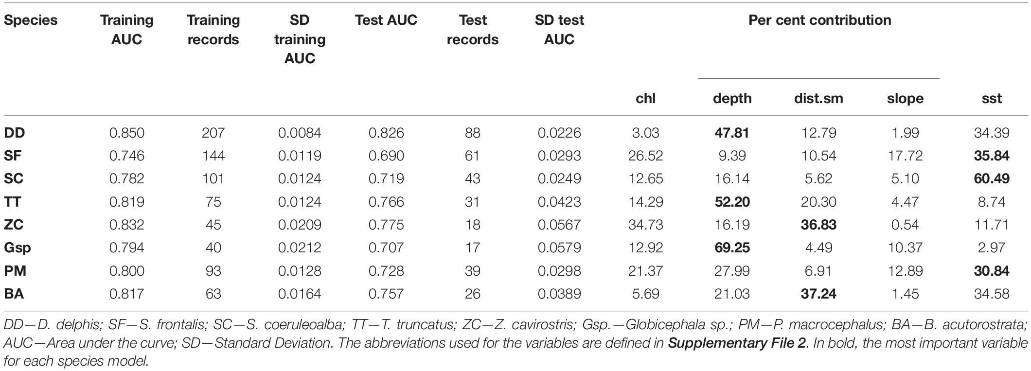
Table 2. Results from the Maxent models developed for the eight most frequently sighted species with the 50 km buffer.

Habitat Preferences and Suitability

To interpret the species’ habitat preferences, we used the GAM fitted splines, in the areas of parameter space where the confidence intervals were satisfactory, thus generally excluding the extremities of the functions where confidence limits tend to be widest (Figure 1). The descriptions of habitat suitability across the area are based on the maps obtained with the Maxent models, considering the areas represented by warmer colours as areas of higher habitat suitability and those with colder colours being less suitable or unsuitable habitat, in a percentage scale from 0 to 100% (Figure 2).

FIGURE 2

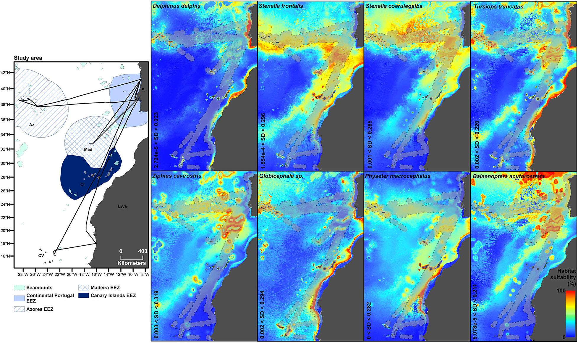
Figure 2. Averaged maps of the eight final niche models obtained with Maxent. The range of standard deviation (SD) of each model is at the bottom left margin of the maps. The 50 km buffer around each presence point is in light grey delimited by dashed lines.

The occurrence of D. delphis, the most frequently sighted species, decreased from the beginning to the end of the summer months. The species was found to be associated with shallower depths and, at the same depth, to locations closer to the coast, and also, at lower sea surface temperatures (Figure 1). These habitats preferences were corroborated by predicted highly suitable habitat occurring mainly in coastal areas with associated upwelling systems, i.e., off continental Portugal and NW Africa, and around the Macaronesian archipelagos (Figure 2).

Similarly, S. frontalis occurrence also decreased throughout the summer months. The species preferred northern waters, contrasting with S. coeruleoalba, the preferred habitat of which decreased toward the north (up to 25°N). Occurrence of both Stenella species peaked at a distance of ∼300 km from the seamounts, at ∼23°C of sea surface temperature, and showed an overall decreasing tendency toward high positive sea level anomalies (Figure 1 and Supplementary File 4). S. frontalis occurrence increased with depth up to 2,000 m, decreasing thereafter (Figure 1). Maxent predictions point to a widespread habitat in the study area for both Stenella species, with higher suitability located mostly in oceanic waters, especially when comparing to the habitat suitability for the other two dolphin species (D. delphis and T. truncatus) (Figure 2).

T. truncatus presented peaks of habitat preferences in different areas: at latitudes ∼15 and ∼35°N, at lower and higher depths, closer to and further from seamounts and at low positive anomalies in altimetry (∼0.05–0.10 cm) (Figure 1). The predicted realised niche pointed to a higher habitat suitability mostly in coastal waters and particularly around the Azores and continental Portugal (Figure 2).

The presence of Z. cavirostris increased from the beginning to the end of the summer months, peaked at ∼35°N latitude, increased with sea depth and decreased toward positive sea level anomalies (Figure 1). The predicted higher habitat suitability of the species was mostly in oceanic areas, with clearly important areas near seamounts, especially those located mid-way between southwest Portugal and Madeira island (Figure 2).

B. acutorostrata had an oceanic occurrence, with preference for areas with depths greater than ∼2,000 m and occurrence generally decreasing toward high positive sea level anomalies (Figure 1). Predicted suitable habitat for minke whales was mainly in oceanic areas, with a clear increase in habitat suitability when in proximity to seamounts (Figure 2), a finding also agreeing with the GAM fitted spline for distance to seamounts (negative relationship with increasing distance to seamounts, Supplementary File 4).

Both Globicephala sp. and P. macrocephalus preferred southern latitudes in the study area. Pilot whale occurrence peaked at ∼1,800 m depth and increased toward high positive sea level anomalies. Sperm whales, at the same depths, had a preference for areas closer to the coast, with an overall increase of occurrence toward areas with higher concentrations of chlorophyll (Figure 1). Higher predicted habitat suitability for both pilot and sperm whales was associated with the continental slope (Figure 2).

Overall, the maps based on Maxent predictions indicated low habitat suitability for all the eight species in oceanic areas which lacked seamounts or islands (Figure 2). All the fitted splines of the eight final best GAM models, including those not illustrated in Supplementary File 4.

Discussion

Cetacean Habitat at Basin-Scale

To our knowledge, this is the first study predicting and mapping suitable habitat for cetaceans, at basin-scale in this region of the eastern North Atlantic, including the high-seas. Many studies focus on cetacean distribution patterns across areas much smaller than their ranging capabilities, thus potentially overlooking the complexity of their biogeographical occurrence patterns (Alves et al., 2018a; García-Barón et al., 2019).

Alves et al. (2018a) illustrated the connectivity of Macaronesia and Iberian Peninsula for one cetacean species (Globicephala macrorhynchus), presenting its wide-range movements, and its spatial structuring, across the entire area. They highlighted the advantages of ecological niche modelling and satellite-linked telemetry to assess the key drivers of the biogeographical patterns in cetacean species occurrence. However, the limitations of ecological niche modelling need to be considered when working with highly mobile species at such a wide scale–we are likely not considering all predictors shaping the species’ distributions: (i) observation data portray only a subset of cetacean occurrence (as cetaceans spend a great amount of time underwater and detectability factors influence data collection); (ii) we are potentially grouping animals at different stages of their life cycle, and/or from different populations or sub-populations (e.g., transient and resident, regional sub-populations) which may have different habitat preferences (Fernández et al., 2013; Correia et al., 2019b; Mannocci et al., 2020), and (iii) those aspects of habitat choice which vary at smaller spatial scales are unlikely to be captured well by a basin-scale model.

In fact, explained deviances of our GAM models were relatively low. Hence, we need to be cautious and avoid over- (or erroneous) interpretation of the results. On the other hand, Redfern et al. (2017) showed that using datasets from multiple (local) ecosystems, i.e., with a wide range of spatial and temporal variability, improves transferability and allows the identification of potentially suitable habitats in data-poor areas, at least if the species’ ecology remains similar to that seen in the ecosystems used to fit the model. In this sense, we are reasonably confident about the transferability of our model predictions as we used a dataset accounting for considerable habitat variability over a wide latitudinal and longitudinal range across the eastern North Atlantic, and we tested the utility of several predictors at multiple scales (Redfern et al., 2006; Fernandez et al., 2018; García et al., 2018).

Cetacean Habitat Preferences and Ecological Niches

Spotted Dolphin and Striped Dolphin

The models, obtained with both techniques, showed the poorest performance for the two Stenella species. Predicted suitable habitat for these species was the most widespread in the area amongst the eight modelled cetaceans. This may indicate that these oceanic dolphins do not have very specific habitat requirements and are more ecological generalists, or that their preferred habitat was not properly sampled. Both hypotheses could explain the low values of deviance explained that were obtained (Brotons et al., 2004).

Common Dolphin

The Maxent model for the common dolphin showed the best performance out of the models for the eight species, with the GAM model explaining about a fifth of the spatiotemporal variation in the occurrence of this species. This is likely related to the fact that the species is the most abundant in the area (e.g., Hammond et al., 2013; Silva et al., 2014; Tobeña et al., 2016; Alves et al., 2018b), with the highest number of sightings among those species used in the modelling process, but it is also relevant that it is an ecological specialist (Marçalo et al., 2018; Correia et al., 2019b). Common dolphins presented clear habitat preferences that limited the predicted regions of highly suitable habitat. The apparent preference for colder waters could be due to either the distribution of suitable habitats mostly in northern latitudes of the study area (northern colder waters) or the preference for coastal areas associated with upwelling systems, located both in the mainland coasts (Portugal and NW Africa) and around the archipelagos. On the contrary, Fernández et al. (2013) reported that common dolphin showed a preference for warmer waters within the northwest Iberian Peninsula. Preliminary analysis of the CETUS dataset, including the first 2 years of surveys along the route from continental Portugal to Madeira, also pointed to a positive tendency of higher occurrence in warmer waters (from 16 to 19°C, stabilising thereafter) (Correia et al., 2015). These results are not necessarily contradictory: the three studies cover very different ranges of surveyed latitudes and, therefore, of surveyed temperatures [Fernández et al., 2013–Galicia; Correia et al., 2015–from North Portugal to Madeira (∼16–∼27°C); and the present study–from Galicia to Cape Verde (∼13–∼30°C)]. This may indicate that within the northernmost part of the study area, at a finer scale, warmer waters are selected by the species. Following the thermal niche theory, as presented by Lambert et al. (2011), it is possible that the waters in northern regions (North of Continental Portugal and Galicia) have temperatures that are marginal in the thermal niche of common dolphins, and hence temperature will strongly influence habitat selection, with the species occurring only in warmer waters. It should be noted though that in the eastern North Atlantic, common dolphins are found as far north as Scotland, likely expanding northwards due to ocean warming (e.g., MacLeod et al., 2005). Over the whole study area (extending as far south as Cape Verde), which comprises mostly warmer waters corresponding to the core temperatures of the species’ thermal niche (>14°C), common dolphins can select more suitable habitats, for example associated with upwelling systems, hence colder waters (but still within the core temperatures). Year-round survey effort is needed to assess seasonal shifts in suitable habitat (i.e., answering the question: where do common dolphins go from autumn to spring?).

Bottlenose Dolphin

GAM models are likely to perform less well, with lower explained deviances, if different populations or ecotypes with varying habitat preferences or habitat uses are being included in the analysis. This may have been the case for the models obtained for the bottlenose dolphin, which has both coastal and oceanic ecotypes in the area (e.g., Fernández et al., 2011; Correia et al., 2020). Nevertheless, clear habitat preferences and areas of highly suitable habitat were found.

The bottlenose dolphins preferred shallower waters in areas where sea depth was less than 4,000 m, but preferred deeper waters in areas where depth exceeded 4,000 m. In areas further from the coast, the species seems to take advantage of the proximity of the seamounts, benefiting from the local upwelling and the lower depths (Pitcher et al., 2007). The preferences also differ depending on the latitudinal range, with a preference for southern areas when between 15 and 25°N, while, from 25 to 35°N, preference increases toward northern waters. The bottlenose dolphin is included in Annex II of the Habitats Directive (Directive 92/43/CEE), hence EU Member States are required to designate Special Areas of Conservation (SACs) for its protection. Moreover, it has also been selected as a priority species to assess indicators for the Marine Strategy Framework Directive. This increases the need for a more complete knowledge of the species’ distribution. Highly suitable habitat includes coastal areas, both for the mainland (Iberia Peninsula and NW Africa) and the archipelagos, with suitable habitats extending further into the high seas adjacent to the mainland. The continental platform and upwelling systems are larger in the mainland than in the archipelagos (Mason, 2009) which may explain the greater extent of suitable habitat in coastal areas of the Iberia Peninsula and NW Africa. These results highlight the need to extend conservation efforts into areas further from the coast. On the other hand, the archipelagos present a narrower continental platform which probably restricts suitable habitat for bottlenose dolphins. Depth was the most important variable for suitable habitat, with bottlenose dolphins mostly restricted to the continental platforms and, when further from the coast, to the seamounts. The majority of these areas are still within the either the Portuguese or the Spanish EEZs. This may facilitate protection measures as individuals occurring within those areas can be included in national management units, reducing the need for (if not the desirability of) cooperation between nations to design a management plan (Santos and Pierce, 2015).

Minke Whale and Cuvier’s Beaked Whale

Minke whales were found mainly in the north of the study area, with suitable habitat restricted to oceanic waters. As in the models for bottlenose, the co-existence of different populations within the area (resident and migratory) may lower the explained deviance of the model. Therefore, research effort should focus on understanding the habitat requirements for migratory vs. resident individuals. Moreover, the movements of the whales (latitudinal and longitudinal) should be further investigated (Valente et al., 2019).

Seamounts were important features shaping habitat suitability for all modelled cetacean species, but their importance was most noticeable for those species occurring most exclusively in oceanic waters –the minke whale and the Cuvier’s beaked whale. Results highlight a very important region of highly suitable habitat: the seamounts of the Madeira-Tore, and specifically the Ampère/Coral Patch Seamounts and the Gorringe Bank. These structures are located between south of mainland Portugal and Madeira island (Dionísio and Arriegas, 2018).

Cuvier’s beaked whale is “data deficient” in European waters and more research effort in the high seas is needed to fill this gap. In fact, large gaps in the environmental space coverage of the eastern North Atlantic were identified, especially in deep and tropical waters (Virgili et al., 2018). We recommend dedicated campaigns coupling acoustic and visual techniques including photo-ID and biopsy collection in the Madeira-Tore (prioritising Ampère/Coral Patch and Gorringe Bank). This could provide baseline data on population density, demography and structuring. Finally, we would recommend surveys during autumn or winter, as the predictions point to an increase of the species occurrence toward the end of the summer season.

Pilot Whale and Sperm Whale

Two species had a clear preference for the south of the study area: pilot whales and sperm whales. For both, habitat suitability was high over the continental slope of the African coastline.

Pilot whales also presented important suitable habitat in the Cape Verde islands. Alves et al. (2018a) demonstrated connectivity of G. macrorhynchus within the Iberian archipelagos but connectivity with Cape Verde or the mainland Africa was not assessed. This should be further investigated to fully understand the species’ movements and population structuring within the study area. Although identification was not achieved to the species level (as both short-finned and long-finned species occur in the area and the two species are almost indistinguishable at sea; Hazevoet et al., 2010; Moura et al., 2017), most sightings were probably of short-finned pilot whale (G. macrorhynchus), given its southern range in comparison with the long-finned pilot whale (Globicephala melas).

For sperm whales, the most important variable was temperature, possibly related to the latitudinal temperature gradient across the surveyed area, with warmer southern waters. However, once this trend was taken into account, occurrence decreased with increasing temperature. As such, it is likely that, within southern (and warmer) areas, sperm whales prefer colder waters (probably associated with upwelling systems; Robinson, 2010). This is also in agreement with the thermal niche theory (Lambert et al., 2011)—sperm whales occurring in waters within the core temperatures of their thermal niche can select preferred habitat characteristics regardless of the temperature. As described in the literature, sperm whales tend to distribute along the continental slope where their preferred prey (cephalopods) are more prevalent (Tepsich et al., 2014). Both Madeira and Canaries have narrower continental platforms than mainland Africa, facilitating the access to the continental slope for research (considering logistics and costs). Along the African continental slope, suitable habitat is most evident in the waters of Western Sahara and Mauritania. In the literature on cetacean occurrence in the NW Africa, Western Sahara is the country for which there is the least information (A. Correia, unpublished data), but in Mauritania, where more research effort exists, sperm whales are indeed reported to have a high prevalence (Camphuysen et al., 2012; Baines and Reichelt, 2014; A. Correia unpublished data). NW African waters suffer from several conservation management issues mostly related to poorly managed or inefficient fishing agreements between African nations and the European Union, with dramatic negative consequences for the marine ecosystems, such as over-exploitation of the fishing resources (Nagel and Gray, 2012; Corten, 2014). Many African countries lack the capacity (e.g., financial) to ensure the conservation of the species in their waters. Hence, given the importance of the area for the eastern North Atlantic sperm whales (and likely for pilot whales as well), conservation of these populations relies on appropriate non-exploitative international support and cooperation. Improved management strategies are urgent to tackle the inevitable increase in human pressures and threats to habitats, such as climate change (Weir and Pierce, 2013).

Overview of the Models

Although it was possible to assess the effects of several environmental variables on cetacean presence, we must highlight that the data were influenced by detectability factors, which emphasises the importance of including such variables in modelling processes and thus taking into account the biases they may cause. As expected, with the exception of S. frontalis, species occurrences decreased with poorer weather conditions (higher wind speed and wave heights, and worse visibility). In the case of S. frontalis, the species is well known for its aerial behaviours, probably more likely when there is a certain amount of surface disturbance (e.g., with moderate wave height), which may cause the species to be easier to spot at a certain sea state—in the present study, the presence of spotted dolphins increased with sea state up to 2, remaining roughly constant thereafter. Since the predictions obtained with Maxent models do not account for weather conditions (as we lack complete spatial data for these variables), the areas of suitable habitat are probably being underestimated: more detections might be made if the weather allowed it.

The ecological meaning of the relationships between species occurrence and chlorophyll-a concentration is hard to interpret, probably due to the temporal (and sometimes spatial) lag inherent to the relationship between chlorophyll measurements and the availability of prey to cetaceans (Frederiksen et al., 2006; García et al., 2018). This lag varies amongst cetacean species according to their prey (i.e., position of the prey/predator in the trophic chain). In previous analyses of habitat preferences for common dolphins, we tested the effect of chlorophyll concentration with various lags (i.e., chlorophyll concentration measured 1 and 2 weeks or months before the date of cetacean observation) and the best model included chlorophyll concentration without lag (Correia et al., 2019b). However, García et al. (2018) found time-lagged chlorophyll concentrations to be useful when modelling the distribution of blue whales in Azores. Thus, we advise testing lagged relationships with chlorophyll concentration in further ecological niche modelling approaches. Altimetry is a proxy for oceanographic processes, such as currents, that alter the ocean surface and cause positive and negative sea level anomalies, mostly related with up- and downwellings due to topographic features and mesoscale eddies (Robinson, 2010). This variable was important in all final GAM models, but the variable was not included when fitting the Maxent models due to its poor resolution. However, it is evident that currents play an important role in cetacean habitat preferences. To improve resolution, other sources of data or proxies should be tested (e.g., in situ measures, current speed or direction).

GAM is a robust technique that supports solid ecological interpretation of habitat preferences, even when working with relatively few sightings. However, GAMs require absence (or pseudo-absence) data, usually implying some sort of survey effort information and often reducing the size of the dataset suitable for analysis. On the other hand, the Maxent technique is widely used to predict habitat suitability with satisfactory results, and it requires only presence data, often significantly increasing the sample size (Redfern et al., 2006; MacLeod et al., 2008a; Derville et al., 2018; Fiedler et al., 2018; Barragán-Barrera et al., 2019). However, Maxent offers few options to estimate the error in the predictions (Phillips et al., 2006). For example, there is no measure of deviance explained, so the explanatory capacity of the model is difficult to quantify, hence this modelling technique is often refered to as “black box” (Phillips et al., 2017). Moreover, since predictor data need to be available for the entire area, the effect of the detectability variables is overlooked. Also, in the present study, due to lack of an adequate sample size by season or month, dynamic variables were averaged and seasonality was lost with Maxent models. Using the two techniques in a complementary approach allowed the integration of the results in order to provide a robust habitat characterisation and interpretation of habitat preferences, an assessment of the detectability influence and seasonality, and the use of the entire dataset to map predictions of habitat suitability (with supporting information of deviance explained, hence explanatory capacity, provided by GAMs, to avoid over-interpretation of results).

Future Directions

Our results are based on data collected mostly during summer, hence interpretations are only applicable for this season. Year-round monitoring would be needed to understand the seasonality of choice of habitats. Seasonality in cetacean habitat preferences has been previously shown (e.g., Fernández et al., 2013). As such, successful marine management may depend on appropriate adaptive strategies for the designation of dynamic Marine Protected Areas (Hooker et al., 2011).

Further endeavours in ecological niche modelling should ideally include other relevant environmental variables (e.g., currents, thermal fronts), consider lags in the oceanographic variables (e.g., chlorophyll concentration), test more spatial and temporal resolutions, and assess geographical variation in species-habitat relationships (Mannocci et al., 2020). This would be ideally done with a bigger dataset, such as would be expected to arise from the CETUS Project as it continues into the 2020s. Modelling should also be performed at finer scales, at least for the areas where highly suitable habitat was predicted, which would require dedicated survey campaigns. Coupling broad-scale and narrow-scale models would improve the understanding of the distribution of suitable habitats. As we stand at the cusp of likely dramatic changes in the marine environment due to climate change, the ecological niche modelling approach should be used to estimate cetacean niches under future climate change scenarios, to support meaningful conservation measures for the cetacean community in the eastern North Atlantic (e.g., MacLeod et al., 2008b; Lambert et al., 2014).

At the deadline of the Strategic Plan for Biodiversity 2010–2020, only 7.4% of the global ocean is protected, against the established 10% target to be achieved by 2020 (according to the last report; UNEP-WCMC et al., 2018). When comparing protection in areas within the EEZs to areas beyond national jurisdiction, the difference is enormous: 16.8% protection against 1.2% (UNEP-WCMC et al., 2018). Furthermore, the increasing impact of several anthropogenic activities on cetacean life history, including shipping traffic, fisheries activity and seismic surveys has been frequently reported (e.g., Azzellino et al., 2017; Kavanagh et al., 2019). Specifically, in offshore waters of the Northeast Atlantic, it has been documented a continuous development of commercial activities in marine areas, together with the lack of management of the use of marine space (European Commission, 2013). Our results have highlighted offshore seamounts as highly suitable habitats for all eight cetacean species, and notably for oceanic bottlenose dolphins, Cuvier’s beaked whales and minke whales. These are areas that need implementation of monitoring programmes and the definition–and implementation–of management plans.

Managing protected areas in the high seas poses several challenges: remoteness limits monitoring and enforcement of measures, transboundary areas require coordinated management across countries, and lack of legislation in areas beyond national jurisdiction calls for adequate international agreements. Cost-effective monitoring programmes, such as the CETUS Project, or programmes based on new technologies that allow remote monitoring (e.g., use of automated vehicles) may be the solution to guarantee the data collection. Ecological modelling approaches or other relatively cheap analysis (e.g., environmental DNA, photo-ID techniques) are potentially suitable methods to support long-term and efficient management and conservation of these remote areas (Bohorquez et al., 2019).

Data Availability Statement

The datasets presented in this study can be found in online repositories. The names of the repository/repositories and accession number(s) can be found below: The dataset analysed for this study can be found openly available in VLIZ, distributed by OBIS and EMODnet at https://doi.org/10.14284/350 – associated data paper (Correia et al., 2019a). Supplementary Material is also provided.

Ethics Statement

Ethical review and approval was not required for the animal study because data used is on visual records of wild ceaceans occurrence only, and no experimentation was undertaken.

Author Contributions

AC was in charge of data collection, processing, analysis, and redaction of the manuscript. DS-G conducted the Maxent models with NS supervision. ÁG and RV were involved in data collection and processing. MR supervised the work and provided assistance in data collection protocol. IS-P was the supervisor and PI of the project under which the data were collected. GP was the lead supervisor of this work and advised on data collection protocol and assisted in data analysis and manuscript redaction. All authors were highly involved in the preparation of this manuscript and reviewed and approved its submission.

Funding

This study was conducted within the Ph.D. program of AC, from the Faculty of Sciences of the University of Porto, Portugal, hosted by the Centre of Marine and Environmental Research (CIIMAR—Porto, Portugal) and funded by the Portuguese national funding agency for science, research and technology (FCT) under the grant SFRH/BD/100606/2014. Two Ph.D. fellowships for authors AG (PD/BD/150603/2020) and RV (SFRH/BD/144786/2019) were granted by Fundação para a Ciência e Tecnologia (FCT, Portugal) under the auspices of Programa Operacional Regional Norte (PORN), supported by the European Social Fund (ESF) and Portuguese funds (MECTES). NS was supported by a CEEC2017 contract (CEECIND/02213/2017). CETUS Project is a monitoring programme, led by CIIMAR | University of Porto in partnership with the cargo ship company TRANSINSULAR | ETE Group.

Conflict of Interest

The authors declare that the research was conducted in the absence of any commercial or financial relationships that could be construed as a potential conflict of interest.

Acknowledgments

We thank all the volunteers for their contribution and dedication during the monitoring campaigns. This manscript is a product of the work of every observer who participated in the CETUS Project. We are extremely grateful to TRANSINSULAR, the cargo ship company that provided all the logistic support, and to the ships’ crews for their hospitality. We also thank Vasilis Valavanis for his valuable advice about the use of oceanographic variables.

Supplementary Material

The Supplementary Material for this article can be found online at: https://www.frontiersin.org/articles/10.3389/fmars.2021.643569/full#supplementary-material

Footnotes

References

Alves, F., Alessandrini, A., Servidio, A., Mendonça, A. S., Hartman, K. L., Prieto, R., et al. (2018a). Complex biogeographical patterns support an ecological connectivity network of a large marine predator in the north-east Atlantic. Divers. Distrib. 25, 269–284.

Google Scholar

Alves, F., Ferreira, R., Fernandes, M., Halicka, Z., Dias, L., and Dinis, A. (2018b). Analysis of occurrence patterns and biological factors of cetaceans based on long-term and fine-scale data from platforms of opportunity: Madeira Island as a case study. Mar. Ecol. 39:e12499. doi: 10.1111/maec.12499