Rapid Assessment of Seabed Habitats Around Pitcairn Island in Aid of Activity Management During the COVID-19 Global Pandemic

The global COVID-19 pandemic of 2020 has forced small island states to make rapid changes to the way they manage their marine estates following changes in global shipping practices and access which are essential for the supply of food items and island’s infrastructure. Following the closure of the border of neighboring French Polynesia, changes had to be made to the Pitcairn Islands’ sole supply vessel route, which resulted in the vessel requiring to set anchor on arrival at the island to conserve fuel. Considering this change and to ensure the continued protection of vulnerable coral habitats the local government has had to make swift decisions to identify anchoring zones that minimize seabed disturbance. Data collected in January 2020, just prior to the pandemic, were assessed using a rapid assessment method and combined with earth observation data to create the first shallow water (<∼20 m) habitat map of this island. The results show the distribution of vulnerable coral communities and other habitats, achieving an accuracy of 68% compared with previously collected datasets making the results the best available evidence for management purposes. Although the seabed data were not originally collected for this analysis, having both video and stills imagery aligned with global positioning meant a rapid assessment method could be easily applied to the data. The assessment technique used has resulted in the first reliable habitat distribution maps to be produced in a management critical timeframe, providing managers with the evidence they required to make informed decisions relating to the protection and conservation of Pitcairn’s pristine, marine habitats during these unprecedented times.

Introduction

Over the past decade “Large Ocean States” have been the main driver behind the creation of large scale marine protected areas (MPAs; Chan, 2018). By the end of 2020, all but one of the top 10 largest MPAs by area, whether sorted by highly protected or mixed-use categories, can be found around these large ocean states or autonomous territories (MCI, 2020). Although highly ambitious there can be difficulty in managing these extensive areas with many of these large ocean states having small populations and very small teams of scientists, marine managers, and enforcement staff (Jones and De Santo, 2016). Changes in the environment and in human behavior create additional challenges for marine managers which need to be overcome to ensure that these valuable areas can remain or become productive and healthy.

For many of these Large Ocean States climate change and the associated pressures will be the main driver behind management in the future. The predicted increase in extreme weather events under current climate change scenarios (IPCC, 2018) will mean managers are going to need to react quickly to changing situations to ensure that their marine environment is protected against negative impacts. Threats to fish populations, tourism opportunities and the removal socio-economic benefits to the local and international population will have to be answered (Forster et al., 2014; Browning et al., 2019). To counter the impact of extreme weather and climate, management measures are tailored toward building ecosystem resilience and ensuring that recovery can take place unimpeded by ongoing human activities that could have a negative impact on the marine ecosystems (McMillen et al., 2014; Anthony et al., 2015).

Human pressures can be managed more directly through restrictions and legislation which are designed to reduce the impact of each activity on coastal ecosystems. Where natural or climatic pressures occur in the same spatial and temporal zone as more direct human pressures, there can be a cumulative impact on the ecosystem (Judd et al., 2015). Although little can be done by local managers to reduce the immediate pressure from a natural/climatic source, such as following a cyclone, managers can reduce the overall impact on the ecosystem by focusing their efforts on reducing the pressure from direct human activities such as extractive or polluting activities (Anthony et al., 2015). To ensure that situations are not exacerbated by management decisions, it is important that managers have access to the best possible evidence (Hayes et al., 2019). It is preferable to gather all the available evidence needed to make those decisions and where the evidence base does not exist, new data are collected to inform the decision (Shucksmith and Kelly, 2014). Following a storm event or the onset of a global pandemic, it may not be possible to collect new data. In these situations, being able to make use of existing datasets to meet the demands of the decision-making process can help reduce the immediate need for new data (Addison et al., 2018).

The Pitcairn Islands are a group of islands located in the central South Pacific, consisting of one volcanic island and three coral atolls. Of the four islands only the second largest, Pitcairn Island, is inhabited with a resident population of approximately 52 (GPI, 2020). The Pitcairn Islands are home to some of the most southerly warm water coral reef systems in the world. Across the four islands 87 species of hard coral have so far been recorded (Irving and Dawson, 2012). Pitcairn Island, being the most southerly, has only 24 recorded coral species. Coral cover at Pitcairn Island is much lower than the other three islands of the group with an average coverage of 5.2% compared to 56.3% at Ducie, 27.8% at Oeno, and 23.5% at Henderson (Friedlander et al., 2014). The comparatively low coverage at Pitcairn Island is likely to be associated with the cooler more southerly latitudes and the high densities of macroalgal species resulting from rain induced run-off (Irving and Dawson, 2013). The most abundant species at Pitcairn Island are Pocillopora verrucosa, Porites lobata, Pocillopora eydouxii, and Millepora platyphylla (Friedlander et al., 2014). Coral cover can range from 5 to 80% with several high density coral cover areas recorded off the north-east and east of the island (Irving and Dawson, 2012). The remainder of the habitats are dominated by macroalgae species including the species Lobophora variegata, Halimeda minima, and the encrusting Lithophyllum kotschyanum (Friedlander et al., 2014).

All imports to the islands arrive via a supply vessel that runs between the Pitcairn Islands and New Zealand and transports people on and off the island via the nearest airport in Mangareva over 500 km away in French Polynesia. Following the global outbreak of the COVID-19 pandemic, the borders of neighboring French Polynesia were closed to the supply vessel, restricting the movement of people off the island. To maintain the needs of the islanders, the frequency of the supply run between New Zealand and Pitcairn was increased. However, to conserve fuel and ensure this route remains financially viable, the supply vessel needed to set anchor while at Pitcairn Island. Previously, due to the quick turn-around times while at Pitcairn and Mangareva there was no need to anchor. Although, anchorages are charted around the island, these are not based on ecological data and just on suitable holding grounds and shelter. Concern has been previously highlighted about the potential impact of anchoring at Pitcairn Island from the supply vessel, visiting yachts and cruise ships (Dawson et al., 2017).

Although previous diver-based investigations of benthic assemblages have taken place around Pitcairn Island, no attempt at describing the full spatial distribution of the different benthic habitats has been undertaken. There is a lack of evidence for the placement of safe anchoring zones which will not impact the potentially fragile coral habitats. The establishment of new “no anchor zones” were a priority of the Government of the Pitcairn Island. However, the urgency which has been brought about by the changing situation caused by COVID-19 has meant that community and substrate information was required to inform the decisions around anchoring quickly. Seabed video, for the analysis of benthic species and habitats, is collected widely by many institutions studying the marine environment. Following collection, analysis can range from an expert assigning a general habitat classification, to identifying and counting each individual seen in the data. The different analysis methods vary in the resolution of detail which is garnered and the time it takes to undertake the analysis with speed often being a trade-off for detail (JNCC, 2019).

The method used here to analyze existing datasets tries to strike a balance between gathering enough information on habitat types and abundance of key species to make an informed decision and the requirement to produce usable maps within less than a month. The study used benthic video data, combined with high resolution earth observations (EO) data already held by the island, to create a new substrate/habitat map for the shallow area around Pitcairn Island. The results of this were then used by the Government of Pitcairn Islands to manage the anchoring around Pitcairn and ensure the protection of vulnerable habitats.

Materials and Methods

Earth Observation Images

Seabed video stations of the original survey were positioned following interpretation of multispectral EO data collected by the European Space Agency’s Sentinel 2A instrument on August 29, 2019. Data was received as Level 2 processed to bottom-of-atmosphere reflectance at a resolution of 10 m.

Higher resolution EO data, obtained for a previous project was used to increase the resolution of the maps. The multispectral data from the WorldView 2 instrument dating from May 11, 2018, arrived as two tiles, a western tile and an eastern tile, with a horizontal resolution of 1.6 m and had been pre-corrected to the bottom-of-atmosphere reflectance. The data underwent several processing steps including cloud and land masking and sun glint correction before being used for mapping. Three new layers were also created using the depth invariant index to remove the impact of the water column. Differences in the spectral values between the two tiles meant that they could not be confidently merged resulting in the tiles being processed separately with the final classification maps merged at the end to form the final full coverage map. To ensure that the 2018 data still represented what was identified during the 2020 survey a comparison of low-resolution open access datasets was made.

Data collected around the same time as the high-resolution data (Sentinel 2A from February 25, 2018) and data from around the time of the video survey (Sentinel 2A from February 5, 2020) were compared. Comparisons were made using a multitemporal change detection method based on outlier detection (Desclée et al., 2006), although for this study the comparison was not tested for accuracy as data was not available. A low level (4.3% of the survey area) of statistically significant change in spectral values had occurred between the datasets. Visual interpretation of the identified changed areas indicated that many of the changes are likely to have resulted from misregistration between the two datasets and not from actual changes in the seabed. Changes in the seabed between 2018 and 2020 was therefore felt to be small enough to not cause problems in the mapping process.

Seabed Video Data

Seabed video data were collected by Joint Nature Conservation Committee (JNCC) and Centre for Environment, Fisheries and Aquaculture Science (Cefas) between 12 and 17 January 2020 during a seabed groundtruthing and coral reef monitoring expedition to the Pitcairn Islands. A total of 58 camera tows were completed during the expedition to gather data to feed directly into the management of the marine environment within the Pitcairn MPA.

The equipment was deployed from the vessel “Via Papa,” an open 6 m local vessel primarily used for fishing the inshore waters around Pitcairn. Seabed video was collected using a drop-down camera frame fitted with a GoPro Hero 7 video camera and an Olympus TG-5 stills camera fitted with a strobe flash. The frame was also fitted with two lasers for scaling images. However, due to the ambient light in the water the lasers were found to be ‘flooded’ out of most of the video. The drop frame was guided to the seabed using a mobile fish finder which allowed the user to maintain the frame approximately 1–2 m above the seabed. Once near the seabed the vessel and drop-down camera frame drifted with the prevailing wind for 10 min resulting in video tows of between 100 and 300 m depending on conditions.

Stations were positioned following interpretation of lower resolution Sentinel 2 data. The blue band, which has greatest depth penetration, underwent an unsupervised classification using the mean-shift segmentation and ISO unsupervised classification tools in ArcGIS v10.5 to split the seabed into classes of similar spectral properties (Esri, 2019). Stations were positioned randomly within each of these classes with the proportion of stations reflecting the total area coverage of each class (Figure 1). Upon request from the Government of the Pitcairn Islands ten stations were placed within Bounty Bay, just off Adamstown Harbour, with seven stations positioned in an area being considered for the placement of a permanent mooring for the supply vessel. Seabed videos were originally collected to assess the coral and other benthic communities around the island. The videos were collected in a manner that allowed individual colonies to be identified to the lowest taxonomic level and to monitor the health of the coral habitats. The total number of stations was limited by the time available to the survey team. The remoteness of the Pitcairn Islands meant that there was a fixed window between supply vessel runs in which the survey could take place.

FIGURE 1

Figure 1. Sampling locations around Pitcairn Island based on a random stratified design using the unsupervised classification of Sentinel 2A multispectral data as the units. The different colored areas represent the six predicted habitats/classes (0–5) which were grouped based on similar spectral properties of the blue band.

Video Analysis

The seabed video underwent a “rapid assessment,” recording the relative abundance of several key species. Species abundance was recorded using the SACFOR scale, which is used to estimate numbers or benthic coverage based on the typical size of the species (Hiscock, 1996). The scale was developed to support the observations of marine organisms in a semi-quantitative manner and provides a means of comparing the abundance and coverage of different species. The scale runs:

• Super-abundant (S)

• Abundant (A)

• Common (C)

• Frequent (F)

• Occasional (O)

• Rare (R)

The size of the individuals and whether the species is encrusting or massive play a part in how the scale is associated with coverage and total numbers (Table 1). This makes it possible to compare different morphotypes quickly and easily based on their impact on the scene.

TABLE 1

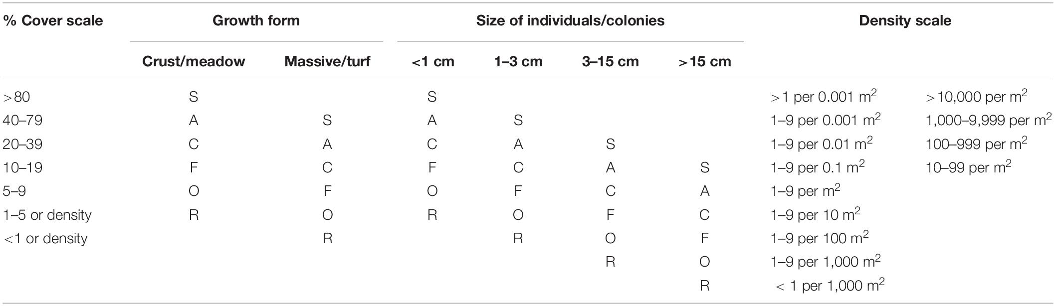
Table 1. The SACFOR abundance measure and how it is applied to different morphotypes and size classes. From Hiscock (1996).

The benthic groups which were selected for the rapid assessment were primarily based on the management needs to identify areas of coral for protection. Additional classes were based on reviews of previous studies around the island and on the survey scientists’ experience in the field. The five taxonomic groups identified were: hard corals, hydrocorals, macroalgae, pencil urchins, and holothurians. Although hard corals and hydrocorals often perform the same ecological role, they were reported on separately here following the guidelines set out by Global Coral Reef Monitoring Network (GCRMN) where hydrocorals are reported in the “Other” category (Moritz et al., 2018). Proportions of sand and rock, as an estimate of percentage cover, were also recorded for each transect. Videos were watched at 1× speed allowing the analysis of all the video data to occur over a few days. The semi-quantitative analysis of the video data was undertaken by four different operators. To ensure consistency between the operators, 10% of each person’s videos were re-analyzed by another operator.

Results from the analysis using the SACFOR scale cannot directly be used for statistical analysis and require conversion into numbers. Here we applied the method developed by Strong and Johnson (2020) which uses the lowest possible count for each category based on size of the individuals and percentage cover and then transforms these numbers by base 10 for counts and base 2 for percentage cover. The results of the video analysis were imported as a species matrix into Primer v7 (Clarke and Gorley, 2015) for interpretation. Multivariate analysis was undertaken to determine the groupings of the transects based on the benthic species abundances and thus the communities present in each video. The Cluster routine was undertaken within Primer producing a dendrogram showing the splits in the data and the similarities between transects at a 5% significance level based on Bray–Curtis similarity. Stations identified as an outlier by the Cluster routine were excluded from the analysis. The clusters were assigned different habitats based on the dominant species and underlying substrate.

Habitat Mapping

The new habitat map was created using object-based image analysis with a supervised classification approach, which used the information gained from the multivariate analysis of the seabed video data to train a predictive model. The input layers into the model included pre-processed high resolution EO bands, depth corrected EO layers (depth invariant index), bathymetry and a directional layer. These layers underwent an image segmentation to divide into objects with the aim of representing real world objects. A classification model was trained using the processed video data and used to predict habitats up to the limits of the EO data.

De-glinting

Sun-glint, off waves and ripples, can impact the mapping process by influencing the signal in the EO data and obscuring the seabed reflectance (Monteys et al., 2015). The impact of sun glint can be removed following the method derived by Hedley et al. (2005). Linear regression was performed separately for the coastal, blue, green and red bands against the near-infrared (NIR) values for an area selected over deep water with a visible glint. De-glinted radiance was calculated by subtracting the slope of the linear regression from the visible radiance values for each pixel (Equation 1).

$$R_i^{\prime }=R_i-b_i(R_{NIR}-Mi{n}_{NIR})(1)$$

Where the pixel value for band i (R_i) is reduced by the product of the regression slope (b_i) and the difference between the pixel NIR value (R_NIR) and the minimum NIR value for the sample area (Min_NIR).

Depth Invariant Index

The attenuation of light with depth can impact on the ability to accurately map different habitats and substrates across different depths. To remove the impact of the attenuation, EO data can be depth corrected based on the ratio of attenuation coefficients from pairs of bands (Leon and Woodroffe, 2011). The method developed by Lyzenga (1981) to correct water column attenuation has the advantage of not requiring depth information to undertake the correction. The correction is undertaken by first identifying areas on the image of the same substrate (e.g., sand) at unknown but different depths. The values for the different bands are log-transformed and then regression of the band-pair values is undertaken. The slope of the regression (k_i/k_j) is then used to calculate the depth invariant index band combination (Equation 2).

$$DI{I}_{ij}=\ln \left(L_i\right)-\left[\left(\frac{k_i}{k_j}\right)\text{ln}(L_j)\right](2)$$

Where L_i is the reflectance of band i, L_j the reflectance of band j, k_i is the attenuation coefficient for band i, and k_j is the attenuation coefficient for band j.

For the current study new depth-invariant layers were created using the following band combinations: Coastal:Blue; Coastal:Green; and Blue:Green for both tiles.

Direction and Bathymetry Layers

Two additional layers were created to supplement the spectral layers; a direction layer and a bathymetry layer.

The direction layer was created to account for any preference for habitats to occupy on one side of the island. Levels of exposure to wave energy, tidal currents, nutrient and freshwater inputs have a strong influence on the distribution of different habitats and species (Brown et al., 2011). Through discussions with local boat operators, it was identified that there may be differences in where habitats are found associated with the exposed and sheltered sides of the islands. Prevailing surface currents which affect all four islands are from the north-east (Irving, 1995). The direction layer was created by assigning each pixel in the EO layers an angular direction to the center point of the island using the Euclidean Direction tool in ArcMap v10.5. This was a proxy for the different levels of exposure which, if time and data were available, would be included with hydrodynamic or wave models.

The bathymetry layer was created using the method derived from Stumpf et al. (2003) and uses the ratio between the natural logarithm of two different wavelengths of light (Equation 3). The ratio approach makes use of the difference in attenuation of blue and green wavelength light through water and has shown to be a reliable bathymetric mapping methodology over variable substrates.

$$depth=m_1\frac{\ln \left(n{R}_W\left({\mathrm{\lambda }}_i\right)\right)}{\ln \left(n{R}_W\left({\mathrm{\lambda }}_j\right)\right)}-m_0(3)$$

Where m₁ is the slope between the ratio layer and the actual depths and m_o is the intercept; n is a fixed constant to assure that the logarithm will be positive.

Depths collected using the fish finder during the survey were used for the regression. As these depths were not corrected for changes in sound velocity through the water column or corrected for tides the resulting bathymetry layer is only suitable for contextual information and not for absolute values.

Object-Based Image Analysis

Object-based image analysis (OBIA) is a method of mapping based on computer vision which aims to delineate real-world items from remote sensing data and combine image processing and geographical information services (GIS) to use the spectral and contextual information in an integrated approach (Blaschke, 2010). In its simplest form OBIA involves the segmentation of the remote sensing data into objects which are then classified, either manually or using a classification algorithm.

The depth invariant layers and the processed coastal bands were loaded into the image processing software eCognition v9.3 (Trimble., 2018) at their original resolution of 1.6 m. This software was used in preference to ArcMap for the mapping steps, which was used in the planning stages, due to the ability to build complex process trees and test each step during the build. Image segmentation was carried out using the multi-resolution segmentation algorithm within eCognition which has shown to perform well when working with subtidal remote sensing data (Roelfsema et al., 2013, 2018). This is an optimization procedure that starts with an individual pixel and consecutively merges it with neighboring pixels to form an object. The process continues until a threshold value for a scale parameter determining the variability allowed in the objects is reached. For the segmentation the coastal band and the Depth Invariant Blue:Green layer were equally weighted with the other layers not used for the segmentation. The segmentation parameters were set to a scale parameter of 10 with shape and compactness set at 0.5. The scale parameter was derived from the visual inspection of the results of the segmentation using different scale parameters (1, 2, 10, 20, 30, and 50). The scale parameter of 10 appeared to represent the real-world objects in the EO data best and was used for both tiles.

The multi-resolution segmentation was set to over-segment the layers to ensure real world features were not missed. A region growing segmentation algorithm was then used to fuse objects of similar properties to form larger objects which are representative of what was seen in the remote sensing data. Habitat information was attributed to the map using the derived communities identified from the multivariate analysis based on the central location of the camera transect. Objects which coincided with the central location of the transect were tagged with the community. These tagged objects became the training dataset for the supervised classification of the remaining unclassified objects. Of the 65 samples which were processed for habitat type, 49 fell within the limit of the high-resolution EO data and were used for the classification of the data. Statistics based on the attributes of the classified objects were exported from eCognition and assessed for classification model fitting in R programming language (R Core Team, 2013). The statistics exported included the mean object value for the depth invariant values for Coastal:Blue; Coastal:Green; and Blue:Green along with the mean object values for coastal band, depth and directional layer. The within object standard deviation was also exported for all the layers.

For both tiles conditional inference trees were calculated based on the object statistics using the “party” R package. Conditional inference trees are a non-parametric class of decision tree and use recursive partitioning of dependent variables based on the values of correlation (Hothorn et al., 2006). The output from a conditional inference tree is relatively simple to understand and allows the user to easily translate the splits into a rule set for classification (Diesing, 2016). As the number of video transects was fairly low within this study there is a chance the splits that the model has created may not truly reflect the whole study area. Using expert interpretation, the splits can be adjusted slightly to more truly reflect the differences seen in the EO data. The conditional inference tree for the western tile was created first with the splits then being applied to the unclassified objects from the segmentation. For the Eastern Tile, the training dataset was supplemented using the classified objects from the Western Tile which overlapped the image. These overlapping objects were included in the segmentation of the Eastern Tile as a thematic layer. The conditional inference tree for the eastern tile was created and the splits applied to the unclassified objects.

Manual editing was applied to areas where classes had over-predicted a habitat, with this being particularly apparent in transitional areas. In total, 0.25 km² of the map was manually edited which equated to 2.53% of the total area mapped.

Consistency and Accuracy

As the map consisted of two tiles, which were mapped independently, all of the 2020 video data were used within the classification methodology to ensure that all of the classes were sufficiently represented. Therefore, no new samples were withheld from map creation to independently assess map accuracy. Instead, indicative assessments have been made against historical datasets collected using different methods and from different times. Two datasets were used for the comparison. The first was collected in 2012 as part of the National Geographic Pristine Seas Expedition (Friedlander et al., 2014), which undertook diver transects at 26 locations around Pitcairn Island. The second dataset was collected as part of a Darwin Initiative funded project looking at fish stocks (Duffy et al., 2021), which collected video data using baited remote underwater video cameras at 37 locations within the mapped area. As the datasets were collected and analyzed using different methods comparisons are made against the estimated habitats from each dataset against the derived habitats from the analysis here to give an indicative accuracy assessment.

Results

Community Analysis by Rapid Assessment

A total of 58 video transects were analyzed based on the rapid assessment method using the SACFOR abundance scale. No differences in use of the SACFOR scale between the different operators were found. The low number of easily identifiable taxa selected for analyses meant no further re-analysis or alteration of the dataset was needed. During analysis it was identified that there were seven transects where the substrate type changed notably for over 2 min of the 10 min videos (e.g., 100% rock to 100% sand). Where this occurred the transects were divided into two and re-analyzed as two transects. This led to 65 samples being imported into Primer for analysis.

The multivariate analysis identified six clusters along with four outlier stations at a 5% significance level. Based on similarities between the contributing species, identified from the Simper analysis, and the underlying substrates, two of the clusters were combined. The final five clusters are described in Table 2; the habitat description is based on the community analysis, majority underlying substrate, and visual interpretation of the relief.

TABLE 2

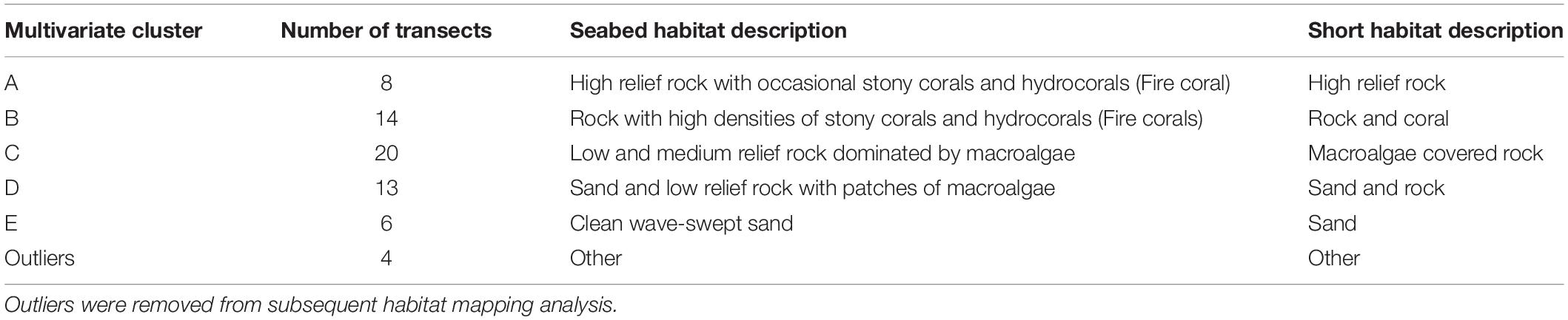
Table 2. Results of the multivariate clustering with the number of transects for each cluster and a habitat description based on the substrate and characterizing taxa.

Macroalgal species were present in all five habitats, dominating three of them (Figure 2). The low abundance of macroalgae found in the Sand habitat occurred on infrequent isolated stones and outcropping rock within the habitat. Stony corals dominated two of the habitats, “rock and coral” and “high relief rock,” both in terms of abundance and contributions to within cluster similarity. Low abundances of stony coral were also found within the “macroalgae covered rock” and “sand and rock” habitats but did not contribute more than 6% to within cluster similarity. Hydrocorals, which were mostly dominated by Millepora spp., were found in all the habitats associated with rocky substrates with the highest abundances seen in the “rock and coral” habitats.

FIGURE 2

Figure 2. Transformed average abundances for the five taxonomic groups within the five derived habitat classes. The size of the bar indicates the transformed abundance of each taxonomic group while the percentages show the contribution of each taxonomic group to within cluster similarity.

No incidences of anchor damage were identified from the video data. However, this was not part of the primary objective during the analysis so subtle signs of damage may have been overlooked.

Locations and Extents of Habitats in New Habitat Map.

Maps of the five habitats observed within the shallow waters of Pitcairn Island are presented in Figure 3; with the limits of the mapping extending to the usable EO data (∼20 m depth). “High relief rock” habitats were predicted to occupy the area immediately off the shore around the majority of the island, excluding the southwest side, and stretch to approximately 150 m from the shoreline. “Rock and coral” habitat, with high densities of stony and hydrocorals, was mostly predicted to occur to the south-east of the island. “Macroalgae covered rock” was the most widely spread, accounting for over a third of the total area mapped. This macroalgae dominated habitat was found around most of the island with the largest areas to the south and south-west of the island. The habitat “sand and rock,” which had similar characteristics to “macroalgae covered rock” but with lower densities of macroalgae, was found to occur more on the northern side of the island and also between the rockier areas to the south-west. Patches of clean wave-swept sand were predicted to occur around the island and were typically found around 200 to 300 m off the shoreline. To the north of the island these patches of sand extend into the deep regions and are likely to extend beyond the limits of the map here, with video transects showing sand in the deeper regions to the north and west of the island.

FIGURE 3

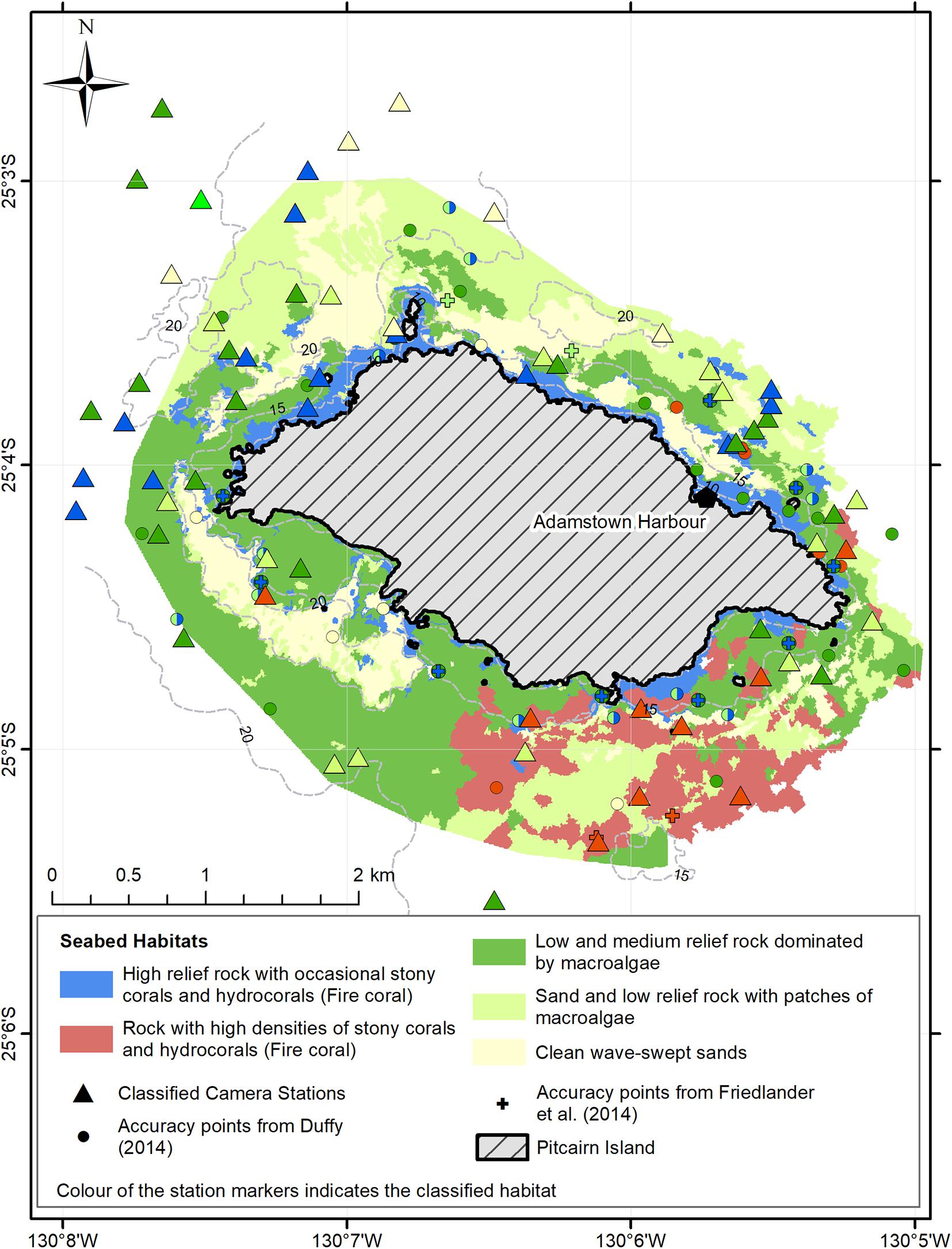
Figure 3. Spatial distribution of the five habitats around Pitcairn Island with the limit being approximately the 20 m depth contour. Individual points for the classified video samples and the historical datasets used for assessing accuracy are also displayed.

Accuracy Assessments

The accuracy assessments were based on the relationship between the estimated habitats from the historic datasets and the predicted habitats created within this study. A relationship table between the three studies was used to convert the habitats from the current study into the estimated habitats of the two historical studies (Table 3). The habitat classifications from this study were converted to those of the historical studies to undertake the accuracy assessment. Out of a total of 63 data points [26 from Friedlander et al. (2014) and 37 from Duffy et al. (2021)], 43 (68%) were found to be in agreement with the new predictive habitat map based on the relationships in Table 3. Comparison between the two historical datasets separately produced quite variable results. The comparison with the Friedlander et al. (2014) study showed an accuracy of 96% of samples being in agreement. However, the comparison with the results from Duffy et al. (2021) scored much lower with 49% of samples in agreement.

TABLE 3

Table 3. Relationship between habitat descriptions from the historical datasets and the current predictive maps.

Discussion

This study reveals the spatial distribution of habitats around Pitcairn Island for the first time, giving the island’s administration the evidence, in the form of the first habitat map of the nearshore area, required for effective and evidenced based management. Using a semi-quantitative method for the analysis of seabed video data, five different habitats were identified and then mapped using high resolution multispectral satellite imagery (Figure 3). The initial results were delivered to the Pitcairn Islands within a month of the COVID-19 pandemic interrupting shipping movements. The habitats identified through this study are similar to those identified during previous work (Friedlander et al., 2014; Duffy et al., 2021) but have now been associated with a spatial distribution. The data produced here have fed directly into the management of the anchoring around Pitcairn Island. Although formal “no anchor” zones have yet to be set up, the supply vessel and visiting yachts have been supplied with the new habitat map and asked to avoid areas with high densities of corals which may be damaged through anchoring. At the time of writing plans are in production for the placement of a new permanent mooring for use by the supply vessel and smaller visiting cruise ships. The new data will also help inform the environmental impact assessment for the new mooring.

Agreement between the processed data and the historical datasets was 68% for the overall map. The accuracy for the overall map were similar to studies of subtidal habitat mapping from EO data in tropical and subtropical environments which used a more detailed and time consuming method of seabed video analysis (Baumstark et al., 2016; Collin et al., 2016; McIntyre et al., 2018). However, these studies did undertake quantitative accuracy assessments with data separated into training and testing datasets which we were unable to perform here. When using the new map for management it is important to understand the limitations of the data as this can influence where the use of the map is appropriate and where it is not. This current investigation relies on historical datasets collected in 2012 and 2014 to undertake the assessment of accuracy. The age of these datasets may influence the outcome with potential changes in seabed habitats occurring in the intervening eight or 6 years between studies. In addition to the time differences, the matching of habitats between the current study and the ones identified during the previous studies was also likely to influence the accuracy (Table 3) and is a likely cause for the differences between the separate accuracy assessments. There is a level of subjectivity when matching the habitats between the three studies as both historical datasets used a broader set of classes for their description than was described here. There is likely to be overlap between the classes as the five classes here are matched between the four classes within the two historical datasets. Although the map is considered to be suitable for its intended use, based on the levels of agreement, the indicative nature of the assessment made here should be taken into account when using this map for management and the limitations in the accuracy made clear to the final users.

The use of pre-existing data also came in the form of the use of a pre-owned high resolution EO data collected in 2018. Ideally, the groundtruthing data and the layer which the predictions are made to would be collected simultaneously or as close in time as possible. This allows direct comparisons to be made and removes any temporal error from the map. In this instance new EO data was not acquired as it was felt that little change would have occurred in the shallow habitats around Pitcairn in the intervening 2 years. Statistical comparisons between low-resolution datasets spanning the same time period supported this assumption with only 4.3% of the survey area having significantly changed.

The level of agreement achieved between the new map and historical datasets can be partially attributed to the low number of habitat classifications which were derived from the community analysis. Having only five habitat classes, which are relatively broad in their nature, does mean that some of the information on natural variation and complexity is lost. The balance between the number of classes, habitat diversity and ease of use is an important consideration when building a map for management. Different management decisions require data at different levels of detail (Lecours, 2017). Mismatches in the resolution of impact, management and evidence have been shown to lead to failures in conservation and management (Cumming et al., 2006). The evidence produced here is to support the management of anchoring to protect the coral habitats around Pitcairn. The simple nature of this management advice request, which could be simplified to identifying areas of high coral cover and areas of little coral cover, along with the relatively low species diversity around Pitcairn Island (Irving and Dawson, 2013; Friedlander et al., 2014) fits with the broad scale nature of the habitat classes defined.

Some of the benthic features previously identified around Pitcairn, such as the extensive coral areas around the NE of the island (Irving and Dawson, 2012), were not identified during this study. This is likely to be associated with the depth cut-off used to limit the area mapped within the current study. Previously, these features had been found in water depths between 18 and 30 m, whereas the limits for the current map are around 20 m. This is one of the primary limitations of using EO data to map benthic habitats, in that one is limited by the penetration of light within the water column. The creation of the bathymetric layer using the Stumpf et al. (2003) method provided an extinction depth where seabed reflectance is no longer visible at approximately 20 m, which was then used to clip the predictor layers before applying the classifications. Although the waters around Pitcairn are known to be exceptionally clear, with underwater visibility in excess of 70 m, other factors on the day of EO image collection may have impacted the availability of light. Increased turbidity through surface run-off, waves and sunglint can all decrease the maximum mapping depth (Traganos et al., 2018). Other methods of seabed mapping such as using multibeam echo sounders can be used to further extend these maps into deeper water covering the areas missed by these maps. However, increased costs of equipment, vessel charter and time required to carry out a survey can be prohibitive. Although the new map does have limitations it is still the best available evidence for the management of the shallow waters around Pitcairn Island. The principle of evidenced based management and using the best available evidence are key principles for the effective management of MPAs (Addison et al., 2018; Hayes et al., 2019). As new data are collected and made available this map can be refined and updated to improve its accuracy and its applicability to other management decisions.

Semi-quantitative analysis of video data was undertaken to rapidly identify the different seabed habitats and in identifying habitats which may be impacted by anchoring or the placement of a permanent mooring base. Although the method has been shown to produce results which agree with previous datasets, there are limitations to this method when compared to undertaking a more quantitative approach, such as point counts. Analysis by the Joint Nature Conservation Committee has compared the accuracies of the different benthic image analysis methods including using the SACFOR abundance scale (Moore et al., 2019). Using a standard set of images and taxonomic lists, results using the SACFOR scale were found to be similar in accuracy and power to more comprehensive methods such as grid counts and point intercepts, giving statistically similar results for community analysis. However, it was also found that out of the different methods tested it was one of the least consistent approaches between operators. The SACFOR abundance scale is supported by quantitative thresholds and there is a level of subjectivity when applying these especially to video data. Where multiple scientists are working on the data and classifying video data in a short time frame, it is imperative to quality assure results between operators to ensure consistency. Consistency also improves with experience, training and predefined field methods and examples (Strong and Johnson, 2020). Within this study the low number of taxonomic groups and the relatively low complexity of the habitats around Pitcairn Island meant that inter-operator error was very low when using the method.

Semi-quantitative imagery analyses methods have been used extensively and are embedded in many of the methodologies for monitoring benthic marine ecosystems (Hiscock, 1996; Hill and Wilkinson, 2004; Obura, 2014; Wheater et al., 2020). The method is mainly used for recorded video data from drop-down cameras and remotely operated vehicles (ROVs). In subtropical and tropical locations, a focus on inshore habitats, higher water temperatures and the need for detailed inspections of corals for identification means using divers to undertake transects and quadrat surveys are more typical than the use of drop-down camera systems or ROVs. As such, the majority of methods created for the monitoring of coral reefs and other tropical ecosystems are tailored toward divers undertaking line or belt transects and undertaking the identification of taxa in real time (Hill and Wilkinson, 2004; Obura, 2014). As shown in this study having a permanent record, which can be re-analyzed to suit the situation, allows managers to react to rapidly changing situations with higher confidence. The recent reduction in costs seen for high-resolution waterproof cameras means collection of data from diver surveys can now also include video and stills data with very little additional outlay; allowing a permanent record of the data to be kept for future use.

Future imagery data collection at Pitcairn should employ the same methodology and equipment as this study to ensure data collected going forward can be readily compared to results of this study. More detailed analysis of imagery collected (i.e., segmenting transects by habitat type, quantifying and identifying all taxa present to lowest taxonomic level possible) would allow for more detailed mapping of habitats and for more quantitative assessment of change in biological communities over time. Increasing coverage and number of camera transects across the study area would also improve validation of and confidence in the habitat map.

A standardized method of data collection along with appropriate metadata gives the maximum likelihood that the data can be re-used. During the survey planning stages it is useful to take into account what potential uses the data may have in the future. The mantra of “collect once, use many times” has been widely pervaded as a way of getting added value from often expensive and time consuming marine surveys (Turrell, 2018). The sampling for this survey followed a stratified random sampling design, which is a well-established method (Nobel-James et al., 2018) designed to increase precision by ensuring all of the units, in this case habitats, are adequately represented in the data (Davies et al., 2001). Although international standards for metadata exist, such as ISO 19115 and EU Inspire Directive, even basic information such as time, date and location (coordinates) are invaluable for being able to repurpose datasets.

The unexpected changes that the island has seen during the COVID-19 pandemic created a challenging situation for the Government of the Pitcairn Islands. This new map provides the best available evidence on the spatial distribution of different habitats around the island. Although corals have been shown to be highly sensitive to anchor damage (Giglio et al., 2017), further work on the sensitivity of the corals at Pitcairn Island and other species within the different habitats to anchor damage would further improve the evidence base for any future decisions on the location of no-anchoring zones.

Conclusion

The analysis carried out here demonstrates the use of a rapid assessment method to repurpose pre-existing data to support marine management. The new habitat map produced from the combination of the rapid assessment and EO data provided the first shallow water spatial dataset for Pitcairn Island filling a gap in the evidence needed for effective management. The distribution of these habitats feeds into the decision-making process for Pitcairn Island for the zonal management of anchoring around the island. With increased pressure from climatic sources and changing human behaviors on marine ecosystems, being able to plan surveys which can be repurposed later in the event of a rapid change is essential.

Data Availability Statement

The raw and derived data supporting the conclusions of this article will be made available by the authors and will be submitted to the Cefas Data Hub, without undue reservation (data.cefas.co.uk).

Author Contributions

All authors contributed towards the planning, preparation and implantation of the fieldwork, data analysis and interpretation, and writing the manuscript. SA-R was the PI and lead author. PW, JO’C and AD worked on the analysis and in writing the manuscript.

Funding

The field work was funded through the UK Government Conflict Stability and Security Fund – Official Development Assistance. Earth Observation Data was acquired through funding provided by Defra Marine R&D. Funding for the analysis and writing of the manuscript was provided by the UK Governments Blue Belt Programme administered by the Foreign, Commonwealth and Development Office (FCDO).

Conflict of Interest

The authors declare that the research was conducted in the absence of any commercial or financial relationships that could be construed as a potential conflict of interest.

Publisher’s Note

All claims expressed in this article are solely those of the authors and do not necessarily represent those of their affiliated organizations, or those of the publisher, the editors and the reviewers. Any product that may be evaluated in this article, or claim that may be made by its manufacturer, is not guaranteed or endorsed by the publisher.

Acknowledgments

We would like to thank the Government of the Pitcairn Islands for their support and expert knowledge in the planning and completion of the fieldwork. We would also like to thank Peter Mitchell (Cefas) and Jane Hawkridge (JNCC) for their advice and for reviewing the manuscript in its final draft. The team would also like to thank Alan Friedlander for providing the metadata from their 2012 survey during the initial planning stage which then became so useful during the evaluation stages. We would also like to thank various staff at the JNCC and Cefas for assisting with the logistics in getting our personnel and equipment to and back from the Pitcairn Islands safely.

References

Addison, P. F. E., Collins, D. J., Trebilco, R., Howe, S., Hedge, P., Jones, G., et al. (2018). A new wave of marine evidence-based management: emerging challenges and solutions to transform monitoring, evaluating, and reporting. ICES J. Mar. Sci. 75, 941–952. doi: 10.1093/icesjms/fsx216

CrossRef Full Text | Google Scholar

Anthony, K. R. N., Marshall, P. A., Abdulla, A., Beeden, R., Bergh, C., Black, R., et al. (2015). Operationalizing resilience for adaptive coral reef management under global environmental change. Glob. Chang. Biol. 21, 48–61.

Google Scholar

Baumstark, R., Duffey, R., and Pu, R. (2016). Mapping seagrass and colonized hard bottom in Springs Coast, Florida using WorldView-2 satellite imagery. Estuar. Coast. Shelf Sci. 181, 83–92. doi: 10.1016/j.ecss.2016.08.019

CrossRef Full Text | Google Scholar

Blaschke, T. (2010). Object based image analysis for remote sensing. ISPRS J. Photogramm. Remote Sens. 65, 2–16. doi: 10.1016/j.isprsjprs.2009.06.004

CrossRef Full Text | Google Scholar

Brown, C. J., Smith, S. J., Lawton, P., and Anderson, J. T. (2011). Benthic habitat mapping: a review of progress towards improved understanding of the spatial ecology of the seafloor using acoustic techniques. Estuar. Coast. Shelf Sci. 92, 502–520. doi: 10.1016/j.ecss.2011.02.007

CrossRef Full Text | Google Scholar

Browning, T. N., Sawyer, D. E., Brooks, G. R., Larson, R. A., Ramos-Scharrón, C. E., and Canals-Silander, M. (2019). Widespread deposition in a coastal bay following three major 2017 Hurricanes (Irma, Jose, and Maria). Sci. Rep. 9:7101. doi: 10.1038/s41598-019-43062-4

PubMed Abstract | CrossRef Full Text | Google Scholar

Chan, N. (2018). “Large ocean states”: sovereignty, small islands, and marine protected areas in Global Oceans Governance. Glob. Governance 24, 537–555. doi: 10.1163/19426720-02404005

CrossRef Full Text | Google Scholar

Clarke, K., and Gorley, R. (2015). PRIMER version 7: User manual/tutorial. PRIMER-E 192.

Google Scholar

Collin, A., Laporte, J., Koetz, B., Martin-Lauzer, F. R., and Desnos, Y. L. (2016). “Mapping bathymetry, habitat, and potential bleaching of coral reefs using Sentinel-2,” in Proceedings of the 13th International Coral Reef Symposium (ICRS 2016), Honolulu, HI, 405–420.

Google Scholar

Cumming, G. S., Cumming, D. H. M., and Redman, C. L. (2006). Scale mismatches in social-ecological systems: causes, consequences, and solutions. Ecol. Soc. 11:14.

Google Scholar

Davies, J., Baxter, J., Bradley, M., Connor, D., Khan, J., Murray, E., et al. (2001). Marine Monitoring Handbook. Peterborough: JNCC.

Google Scholar

Dawson, T. P., Gray, K., Irving, R. A., Crick, A., O’Keefe, S., and Christian, M. (2017). Fisheries Management Plan for the Pitcairn Islands Coastal Conservation Areas. Report to the Natural Resources Division. Adamstown: Government of Pitcairn Islands.

Google Scholar

Desclée, B., Bogaert, P., and Defourny, P. (2006). Forest change detection by statistical object-based method. Remote Sens. Environ. 102, 1–11. doi: 10.1016/j.rse.2006.01.013

CrossRef Full Text | Google Scholar

Diesing, M. (2016). “Application of geobia to map the seafloor,” in Proceedings of the GEOBIA 2016 Solutions and Synergies, Enschede. doi: 10.3990/2.405

CrossRef Full Text | Google Scholar

Duffy, H. J., Letessier, T. B., Koldewey, H. J., Dawson, T. P., and Irving, R. A. (2021). Ensuring the sustainability of coastal small-scale fisheries at Pitcairn Island (South Pacific) within a large scale no-take MPA. Front. Mar. Sci. 8:528. doi: 10.3389/fmars.2021.647685

CrossRef Full Text | Google Scholar

Esri (2019). ArcGIS Desktop (Version 10.5).

Google Scholar

Forster, J., Lake, I. R., Watkinson, A. R., and Gill, J. A. (2014). Marine dependent livelihoods and resilience to environmental change: a case study of Anguilla. Mar. Policy 45, 204–212. doi: 10.1016/j.marpol.2013.10.017

CrossRef Full Text | Google Scholar

Friedlander, A. M., Caselle, J. E., Ballesteros, E., Brown, E. K., Turchik, A., and Sala, E. (2014). The real bounty: marine biodiversity in the Pitcairn Islands. PLoS One 9:e100142. doi: 10.1371/journal.pone.0100142

PubMed Abstract | CrossRef Full Text | Google Scholar

Giglio, V. J., Ternes, M. L. F., Mendes, T. C., Cordeiro, C. A. M. M., and Ferreira, C. E. L. (2017). Anchoring damages to benthic organisms in a subtropical scuba dive hotspot. J. Coast. Conserv. 21, 311–316. doi: 10.1007/s11852-017-0507-7

CrossRef Full Text | Google Scholar

GPI (2020). Government of Pitcairn Islands. Available online at: https://www.government.pn/. (accessed November 6, 2020)

Google Scholar

Hayes, K. R., Hosack, G. R., Lawrence, E., Hedge, P., Barrett, N. S., Przeslawski, R., et al. (2019). Designing monitoring programs for marine protected areas within an evidence based decision making paradigm. Front. Mar. Sci. 6:746. doi: 10.3389/fmars.2019.00746

CrossRef Full Text | Google Scholar

Hedley, J., Harborne, A., and Mumby, P. (2005). Technical note?: simple and robust removal of sun glint for mapping shallow-water benthos Simple and robust removal of sun glint for mapping shallow-water. Int. J. Remote Sens. 26, 2107–2112. doi: 10.1080/01431160500034086

CrossRef Full Text | Google Scholar

Hill, J., and Wilkinson, C. (2004). Methods for Ecological Monitoring of Coral Reefs. Townsville: Australian Institute of Marine Science.

Google Scholar

Hiscock, K. (1996). Marine Nature Conservation Review: Rationale and Methods. Peterborough: Joint Nature Conservation Committee.

Google Scholar

Hothorn, T., Hornik, K., and Zeileis, A. (2006). Unbiased recursive partitioning: a conditional inference framework. J. Comput. Graph. Stat. 15, 651–674. doi: 10.1198/106186006X133933

PubMed Abstract | CrossRef Full Text | Google Scholar

IPCC (2018). “Summary for Policymakers,” in Global Warming of 1.5°C. An IPCC Special Report on the Impacts of Global Warming of 1.5°C Above Pre-Industrial Levels and Related Global Greenhouse Gas Emission Pathways, in the Context of Strengthening the Global Response to the Threat of Climate Change, Sustainable Development, and Efforts to Eradicate Poverty World Meteorological Organization, eds V. Masson-Delmotte, P. Zhai, H.-O. Pörtner, D. Roberts, J. Skea, P. R. Shukla, et al. (Geneva: IPPC), 32.

Google Scholar

Irving, R. (1995). Near-shore bathymetry and reef biotopes of Henderson Island, Pitcairn Group. Biol. J. Linn. Soc. 56, 309–324. doi: 10.1006/BIJL.1995.0068

CrossRef Full Text | Google Scholar

Irving, R., and Dawson, T. (2012). The Marine Environment of the Pitcairn Islands. Dundee: Dundee University Press.

Google Scholar

Irving, R. A., and Dawson, T. P. (2013). Coral Reefs of the United Kingdom Overseas Territories. Dordrecht: Springer, doi: 10.1007/978-94-007-5965-7

CrossRef Full Text | Google Scholar

JNCC (2019). The Big Picture–Benthic Imagery Analysis Workshop. Peterborough: JNCC.

Google Scholar

Jones, P. J. S., and De Santo, E. M. (2016). Viewpoint–is the race for remote, very large marine protected areas (VLMPAs) taking us down the wrong track? Mar. Policy 73, 231–234. doi: 10.1016/j.marpol.2016.08.015

CrossRef Full Text | Google Scholar

Judd, A. D., Backhaus, T., and Goodsir, F. (2015). An effective set of principles for practical implementation of marine cumulative effects assessment. Environ. Sci. Policy 54, 254–262. doi: 10.1016/j.envsci.2015.07.008

CrossRef Full Text | Google Scholar

Lecours, V. (2017). On the use of maps and models in conservation and resource management (Warning: Results May Vary). Front. Mar. Sci. 4:288. doi: 10.3389/fmars.2017.00288

CrossRef Full Text | Google Scholar

Leon, J., and Woodroffe, C. D. (2011). Improving the synoptic mapping of coral reef geomorphology using object-based image analysis. Int. J. Geogr. Inf. Sci. 25, 949–969. doi: 10.1080/13658816.2010.513980

CrossRef Full Text | Google Scholar

Lyzenga, D. (1981). Remote sensing of bottom reflectance and water attenuation parameters in shallow water using aircraft and LANDSAT data. Int. J. Remote Sens. 2, 71–82. doi: 10.1080/01431168108948342

CrossRef Full Text | Google Scholar

MCI (2020). MPA Atlas. In: Mar. Conserv. Inst. Available online at: https://mpatlas.org/large-mpas (accessed June 17, 2021).

Google Scholar

McIntyre, K., McLaren, K., and Prospere, K. (2018). Mapping shallow nearshore benthic features in a Caribbean marine-protected area: assessing the efficacy of using different data types (hydroacoustic versus satellite images) and classification techniques. Int. J. Remote Sens. 39, 1117–1150. doi: 10.1080/01431161.2017.1395924

CrossRef Full Text | Google Scholar

McMillen, H. L., Ticktin, T., Friedlander, A., Jupiter, S., Thaman, R., Campbell, J. R., et al. (2014). Small islands, valuable insights: systems of customary resource use and resilience to climate change in the Pacific. Ecol. Soc. 19:44. doi: 10.5751/ES-06937-190444

PubMed Abstract | CrossRef Full Text | Google Scholar

Monteys, X., Harris, P., Caloca, S., and Cahalane, C. (2015). Spatial prediction of coastal bathymetry based on multispectral satellite imagery and multibeam data. Remote Sens. 7, 13782–13806. doi: 10.3390/rs71013782

CrossRef Full Text | Google Scholar

Moore, J., van Rein, H., Benson, A., Sotheran, I., Mercer, T., and Ferguson, M. (2019). Optimisation of Benthic Image Analysis Approaches. JNCC Report, No. 641. Peterborough: JNCC.

Google Scholar

Moritz, C., Jason, V. I. I., Lee Long, W., Tamelander, J., Thomassin, A., and Planes, S. (2018). Status and Trends of Coral Reefs of the Pacific. Honolulu, HI: Global Coral Reef Monitoring Network.

Google Scholar

Nobel-James, T., Jesus, A., and McBreen, F. (2018). Monitoring guidance for marine benthic habitats (Revised). Peterborough: JNCC.

Google Scholar

Obura, D. (2014). Coral Reef Monitoring Manual South-West Indian Ocean Islands. Honolulu, HI: Global Coral Reef Monitoring Network.

Google Scholar

R Core Team (2013). R: A Language and Environment for Statistical Computing. Vienna: R Foundation for Statistical Computing.

Google Scholar

Roelfsema, C. M., Kovacs, E., Ortiz, J. C., Wolff, N. H., Callaghan, D. P., Wettle, M., et al. (2018). Coral reef habitat mapping: a combination of object-based image analysis and ecological modelling. Remote Sens. Environ. 208, 27–41. doi: 10.1016/j.rse.2018.02.005

CrossRef Full Text | Google Scholar

Roelfsema, C. M., Phinn, S. R., Jupiter, S., Comley, J., and Albert, S. (2013). Mapping coral reefs at reef to reef-system scales, 10s-1000s km2, using object-based image analysis. Int. J. Remote Sens. 34, 6367–6388. doi: 10.1080/01431161.2013.800660

CrossRef Full Text | Google Scholar

Shucksmith, R. J., and Kelly, C. (2014). Data collection and mapping–principles, processes and application in marine spatial planning. Mar. Policy 50, 27–33. doi: 10.1016/j.marpol.2014.05.006

CrossRef Full Text | Google Scholar

Strong, J. A., and Johnson, M. (2020). Converting SACFOR data for statistical analysis?: validation, demonstration and further possibilities. Mar. Biodivers. Rec. 3, 1–18.

Google Scholar

Stumpf, R. P., Holderied, K., and Sinclair, M. (2003). Determination of water depth with high-resolution satellite imagery over variable bottom types. Limnol. Oceanogr. 48, 547–556. doi: 10.4319/lo.2003.48.1_part_2.0547

CrossRef Full Text | Google Scholar

Traganos, D., Poursanidis, D., Aggarwal, B., Chrysoulakis, N., and Reinartz, P. (2018). Estimating Satellite-Derived Bathymetry (SDB) with the Google Earth Engine and Sentinel-2. Remote Sens. 10, 1–18. doi: 10.3390/rs10060859

CrossRef Full Text | Google Scholar

Trimble. (2018). eCognition Developer (Version 10.1).

Google Scholar

Turrell, W. R. (2018). Improving the implementation of marine monitoring in the northeast Atlantic. Mar. Pollut. Bull. 128, 527–538. doi: 10.1016/j.marpolbul.2018.01.067

PubMed Abstract | CrossRef Full Text | Google Scholar

Wheater, P., Bell, J., and Cook, P. (2020). Practical Field Ecology: A Project Guide. Hoboken, NJ: Wiley-Blackwell.

Google Scholar