Quantifying the Atmospheric CO2 Forcing Effect on Surface Ocean pCO2 in the North Pacific Subtropical Gyre in the Past Two Decades

Despite the well-recognized importance in understanding the long term impact of anthropogenic release of atmospheric CO₂ (its partial pressure named as pCO₂air) on surface seawater pCO₂ (pCO₂sw), it has been difficult to quantify the trends or changing rates of pCO₂sw driven by increasing atmospheric CO₂ forcing (pCO₂sw^atm_forced) due to its combination with the natural variability of pCO₂sw (pCO₂sw^nat_forced) and the requirement of long time series data records. Here, using a novel satellite-based pCO₂sw model with inputs of ocean color and other ancillary data between 2002 and 2019, we address this challenge for a mooring station at the Hawaii Ocean Time-series Station in the North Pacific subtropical gyre. Specifically, using the developed pCO₂sw model, we differentiated and separately quantified the interannual-decadal trends of pCO₂sw^nat_forced and pCO₂sw^atm_forced. Between 2002 and 2019, both pCO₂sw and pCO₂air show significant increases at rates of 1.7 ± 0.1 μatm yr^–1 and 2.2 ± 0.1 μatm yr^–1, respectively. Correspondingly, the changing rate in pCO₂sw^nat_forced is mainly driven by large scale forcing such as Pacific Decadal Oscillation, with a negative rate (-0.5 ± 0.2 μatm yr^–1) and a positive rate (0.6 ± 0.3 μatm yr^–1) before and after 2013. The pCO₂sw^atm_forced shows a smaller increasing rate of 1.4 ± 0.1 μatm yr^–1 than that of the modeled pCO₂sw, varying in different time intervals in response to the variations in atmospheric pCO₂. The findings of decoupled trends in pCO₂sw^atm_forced and pCO₂sw^nat_forced highlight the necessity to differentiate the two toward a better understanding of the long term oceanic absorption of anthropogenic CO₂ and the anthropogenic impact on the changing surface ocean carbonic chemistry.

Introduction

Since industrialization, the global ocean has been a major sink of the increasing atmospheric CO₂, absorbing ∼25% of anthropogenic CO₂ in recent years (Sabine et al., 2004a; Friedlingstein et al., 2019; Gruber et al., 2019). On one hand, the continuous ocean sink of atmospheric CO₂ (its partial pressure is named as pCO₂air) is changing ocean carbonic chemistry and the ocean carbon cycle (Borges et al., 2005; Cai et al., 2006; Fujii et al., 2009; Landshützer et al., 2013; Wanninkhof et al., 2013; Xiu and Chai, 2014). On the other hand, the resulting ocean acidification has great potential to degrade marine ecosystems and marine biota, particularly the calcifying organisms such as shellfish and corals (Widdicombe and Spicer, 2008; Doney, 2010; Fabricius et al., 2011; Dickinson et al., 2012; Chan and Connolly, 2013; Davis et al., 2017). Both impacts are closely related to the sustainable development of the marine biota and ecology. Therefore, the anthropogenic effect on surface seawater carbonic chemistry and the potential of the ocean in absorbing anthropogenic CO₂ in the changing world are pressing concerns of the environmental research community.

At present, the study on anthropogenic CO₂ at the sea surface is quite limited. Instead, there are many studies on anthropogenic CO₂ in the ocean interior. The anthropogenic CO₂ stored in the ocean exists in various forms of carbon, originating from the cumulative CO₂ emissions from human activities (e.g., fossil fuel combustion, cement production, etc.) since the beginning of the Industrial Revolution. Several chemical and isotopic tracer approaches have been attempted to estimate the size of this pool of anthropogenic CO₂ (e.g., Sabine et al., 2002, 2004b; Lee et al., 2003; Quay et al., 2017; Gruber et al., 2019). However, due to the sparse measurements of chemical tracers in space and time, there is still significant uncertainty in the long-term accumulation rates of anthropogenic CO₂ and the potential of the ocean in continued absorption of anthropogenic CO₂, making it important to investigate the anthropogenic CO₂ variabilities at the sea surface.

One approach for tracking changes in surface pCO₂sw is through the collection of autonomous underway and mooring observations over the global ocean (e.g., Surface Ocean CO₂ Atlas (SOCAT, Bakker et al., 2016; Sutton et al., 2019). Many studies focused on the overall variabilities in surface pCO₂sw and CO₂ flux (e.g., Rödenbeck et al., 2015; Landshützer et al., 2016, 2019; Gregor et al., 2019; Denvil-Sommer et al., 2019; Iida et al., 2020 among others). However, because of the absence of isotope tracers in the autonomous observing systems of surface pCO₂sw, it is very challenging to estimate how much anthropogenic CO₂ emissions is driving measured pCO₂sw. Alternatively, it is known that surface pCO₂sw is affected by both increasing atmospheric CO₂ forcing (mainly caused by anthropogenic CO₂ emissions) and natural oceanic forcing (e.g., driven by oceanic physical and biogeochemical dynamics) (Fennel et al., 2008; Ikawa et al., 2013; Xue et al., 2016). The effect of atmospheric CO₂ forcing on surface pCO₂sw (named as pCO₂sw^atm_forced hereafter) actually refers to the changes of surface pCO₂sw driven by the increase of atmospheric CO₂. Since the increase of atmospheric CO₂ is due to anthropogenic emissions, the changing rates of pCO₂sw^atm_forced in the past decades can be used to infer the interannual-decadal variations of the anthropogenic signals in surface pCO₂sw. Yet the pCO₂sw^atm_forced should be differentiated from the total observed pCO₂sw because of the combination of the natural variability in surface pCO₂sw (pCO₂sw^nat_forced). Here pCO₂sw^nat_forced refers to the remaining pCO₂sw component without atmospheric CO₂ forcing effect, which could be influenced by different physical and biogeochemical processes in the ocean, including the biological activities (i.e., photosynthesis and respiration), ocean warming driven by climate change and anthropogenic CO₂ emissions, and ocean mixing, etc. The effect of all these different processes was regarded as the overall natural oceanic forcing effect on surface pCO₂sw, It should be clarified that, although we regard all these different oceanic processes to be natural, their changes can still not be completely due to “natural” forcing because these changes in 2002–2019 inherently and implicitly contain atmospheric forcing.

Long time data records are needed to quantify the interannual-decadal trends of pCO₂sw^atm_forced and pCO₂sw^nat_forced in the ocean. Indeed, Sutton et al. (2019) analyzed the time scale of trend detection using 40 autonomous mooring time series of total observed surface pCO₂sw over the globe, and found that anthropogenic trend detection requires a minimum 8 and 16 years of data records for the sites studies in open ocean and coastal regions, respectively. However, the current global time series observation network of surface pCO₂sw just starts to approach these time scales, which has made it difficult to track the atmospheric forcing effect for most oceanic environments where the moorings are deployed. Several recent studies attempted to examine the anthropogenic trend in pCO₂sw based on underway measurements in the past decades (Takahashi et al., 2009, 2014; McKinley et al., 2011). For example, Takahashi et al. (2009, 2014) found that pCO₂sw is increasing at varying rates of 1.2 ± 0.5∼2.1 ± 0.5 μatm yr^–1 in different ocean basins. However, the ship-based measurements are quite limited in both spatial and temporal coverage, leading to many uncertainties in the derived rates. More importantly, these rates are not exactly referring to the atmospheric forcing rates of surface pCO₂sw, because of the combination of natural variability (i.e., pCO₂sw^nat_forced) as mentioned above and the difficulty to differentiate and quantify both pCO₂sw^atm_forced and pCO₂sw^nat_forced using in situ observations of surface pCO₂sw alone.

When combined with in situ surface pCO₂sw observations, satellite remote sensing has become an important tool for synoptic estimation of surface pCO₂sw (e.g., Lohrenz et al., 2010, 2018; Hales et al., 2012; Signorini et al., 2013; Bai et al., 2015; Chen et al., 2019). Without a spectroscopic method for direct measurements of surface pCO₂sw from space, it is possible to develop satellite-based pCO₂sw models through correlations with other related environmental variables. A satellite-based surface pCO₂sw model also makes it possible to differentiate pCO₂sw^atm_forced from pCO₂sw^nat_forced. Indeed, satellite data accumulated in the past 20 years show great potential to quantify the interannual-decadal trends of the atmospheric forcing effect on pCO₂sw. However, the past remote sensing studies mainly focused on the retrieval of seasonal surface pCO₂sw (e.g., Lefèvre et al., 2005; Chierici et al., 2009; Zhu et al., 2009; Borges et al., 2010; Jo et al., 2012; Tao et al., 2012; Marrec et al., 2015; Parard et al., 2015; Le et al., 2019), and are quite limited in predicting interannual variability because of their insufficient parameterization of increasing atmospheric CO₂ forcing (Shadwick et al., 2010; Chen et al., 2019). Therefore, the satellite-based pCO₂sw algorithms need to be refined to enable their capabilities in assessing the interannual trends of pCO₂sw^atm_forced and pCO₂sw^nat_forced.

The Woods Hole Oceanographic Institution Hawaii Ocean Time-series Station (WHOTS) near Hawaii in the North Pacific Subtropical Gyre (NPSG) maintains high resolution surface pCO₂sw observations. It provides an important open ocean reference for Hawaiian coral reefs (Dore et al., 2003; Sutton et al., 2017; Terlouw et al., 2019), thus is important to know the interannual-decadal trends of the atmospheric forcing effect on surface pCO₂sw for a better understanding of the long-term ocean acidification and oceanic absorption of anthropogenic CO₂. The WHOTS station was selected mainly because it has sufficient field data records for anthropogenic trend detection as mentioned above. WHOTS is located at station ALOHA (A Long-term Oligotrophic Habitat Assessment) (Karl and Church, 2018) in the NPSG (Figure 1), under the large-scale climate forcing of Pacific Decadal Oscillation (PDO). Several published studies investigated the interannual variability of the upper ocean carbon cycle at this station (Dore et al., 2003, 2009; Keeling et al., 2004; Palevsky and Quay, 2017). For example, based on a 14-year time series (1988–2002) at ALOHA, Brix et al. (2004) found that surface pCO₂sw and isotopic ¹³C/¹²C showed long-term increase and decrease (yet no rates were provided), respectively, and they attributed it to the uptake of isotopically light anthropogenic CO₂ from the atmosphere. Using the same data time series of pCO₂sw at ALOHA, Dore et al. (2003) found that the significant decrease in CO₂ sink in 1989–2001 was driven by the climate variability in salinity (Lukas and Santiago-Mandujano, 2008). Later based on a longer data record of 19 years (1988–2007) at ALOHA, Dore et al. (2009) presented a pCO₂sw increasing rate of 1.88 μatm yr^–1. In contrast, with a synthesis of 35 years of observations in the North Pacific, Takahashi et al. (2006) found the interannual-decadal change in surface pCO₂sw is mostly correlated with the increases of sea surface temperature (SST) and anthropogenic CO₂. Therefore, it is necessary to further investigate the effects of both anthropogenic CO₂ emissions and the climate-driven natural variability in the ocean on surface pCO₂sw. However, to date, no studies have differentiated these two forcing effects.

FIGURE 1

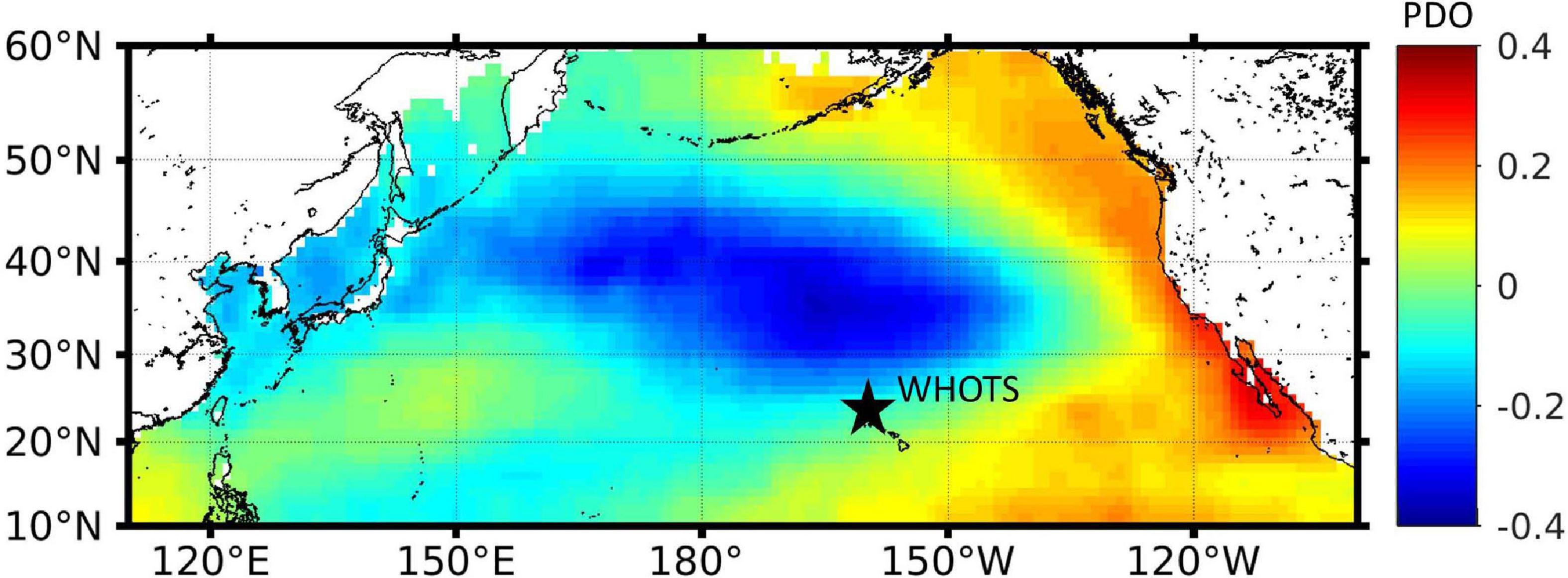
Figure 1. The geolocation of the study site WHOTS (annotated in black star), and the general climate mode of the North Pacific in terms of PDO based on the HadISST data set (Rayner et al., 2003) for the period 1870–2019.

Considering the importance of addressing this knowledge gap to promote our understanding of the ocean capability in absorbing anthropogenic CO₂ in the long run, here we for the first time differentiate the atmospheric forcing and natural forcing effects on surface pCO₂sw, that’s, pCO₂sw^atm_forced and pCO₂sw^nat_forced, based on a novel satellite-based pCO₂sw model developed in this study. Specifically, the objectives of this study include: (1) develop a satellite-based surface pCO₂sw model at WHOTS, which should be able to capture the interannual-decadal variabilities in pCO₂sw and differentiate pCO₂sw^atm_forced and pCO₂sw^nat_forced, and (2) quantify the interannual-decadal trends of both terms in the past 2 decades, and understand its implications for ocean acidification and long term oceanic uptake of anthropogenic CO₂. Although the study was conducted at the WHOTS station, the findings in this study may provide insight on the interannual-decadal trends of pCO₂sw driven by atmospheric and natural forcing effects, respectively, in other global subtropical open ocean regions. More importantly, the approach developed in this study can be extended to other regions with sufficient data available.

Data and Methods

Data

The WHOTS station (22.7°N, 158°W) is located in the subtropical oligotrophic region of the North Pacific and is operated by the Woods Hole Oceanographic Institution (WHOI). Field data time series [including surface pCO₂sw, and pCO₂air, SST, and sea surface salinity (SSS)] at this station collected between 2004 and 2018 at led by NOAA’s Pacific Marine Environmental Laboratory and were obtained from the National Centers for Environmental information (NCEI)¹ (Sutton et al., 2012). Specifically, the pCO₂ data were measured by a non-dispersive infrared gas analyzer (LI-COR^TM, model LI-820), which has a sampling frequency of every 3 h, with an accuracy of 2 μatm (or better) (Sutton et al., 2014; Sabine et al., 2020). Surface pCO₂sw data were collected at a water depth of <0.5 m, and the pCO₂air data were collected at 1.2 m above the sea surface. SST and SSS were obtained from a CTD (SBE16) integrated in the autonomous CO₂ mooring system. The details of data collection, processing, and quality control can be found in Sutton et al. (2014). These data were binned to daily time series to remove the diurnal variations (i.e., 0.4∼3.4 μatm), which are not considered in this study. The data time series were then averaged at monthly scales as presented in in Figures 2A,B,D. The Hawaii Ocean Time-series (HOT) program also maintains ship-based monthly sampling of surface pCO₂sw calculated from dissolved inorganic carbon (DIC) and total alkalinity (TA) at this location (Figure 2D). We chose to use the high-frequency data from the WHOTS buoy mainly to assure that there are sufficient data available to develop the machine learning pCO₂sw model and the monthly averages of the modeled pCO₂sw should have lower bias than the monthly observed pCO₂sw at HOT.

FIGURE 2

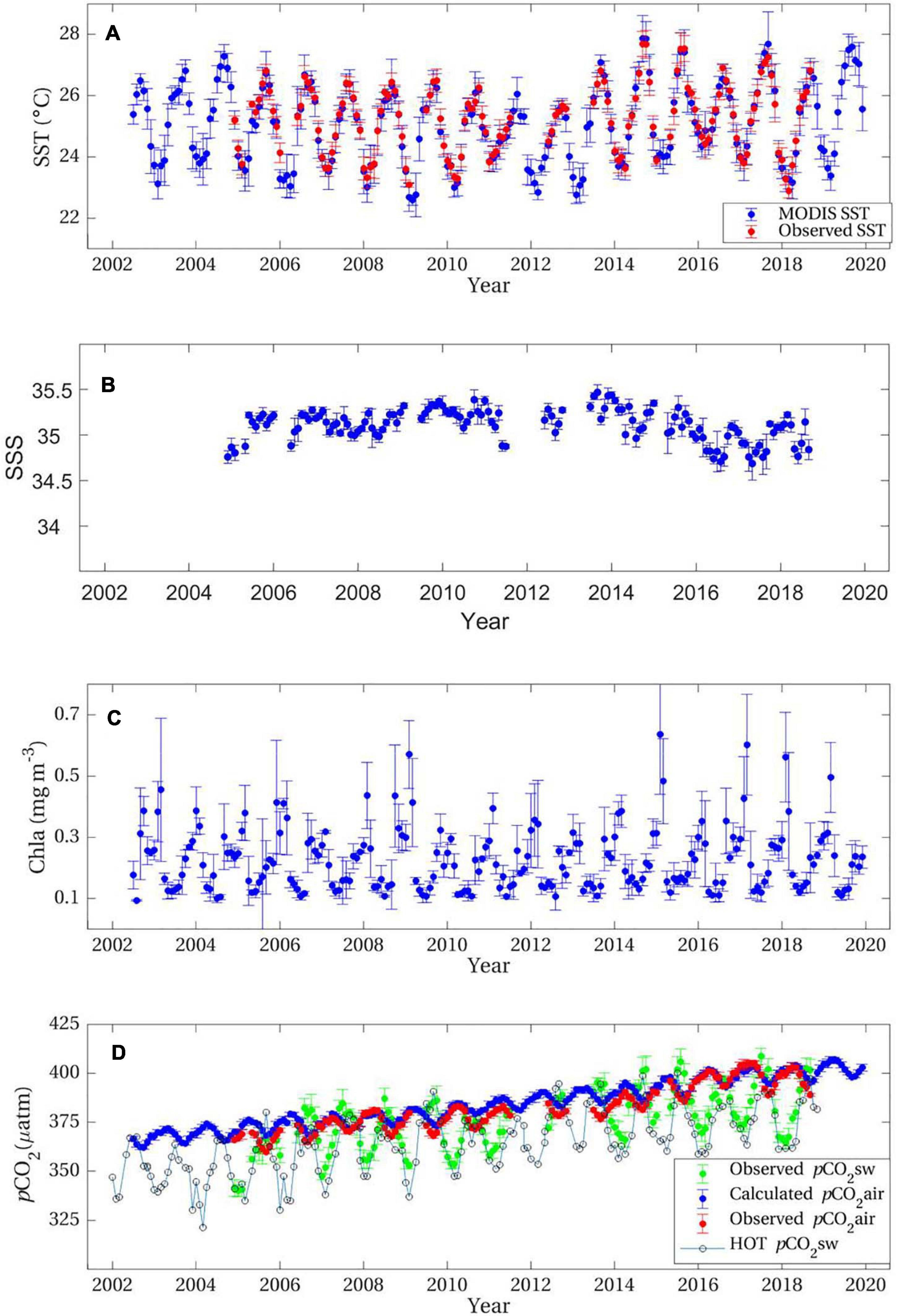
Figure 2. Interannual variations of the monthly SST (A), SSS (B), Chla (C), pCO₂air, and pCO₂sw (D) at the WHOTS station in the period of 2002–2019. Note that the ship-based monthly pCO₂sw time series at HOT calculated from DIC and TA measurements was overlaid in (D) for reference, and the calculated pCO₂air in (D) is based on the data of atmospheric CO₂ measured at MLO.

NASA standard daily SST (Figure 2A) and 8 day Chlorophyll-a (Chla, mg m^–3) (Figure 2C) Level-3 data products (version R2018.0) covering the study region for the period of July 2002–December 2019 with a spatial resolution of ∼4 km were downloaded from the NASA Goddard Space Flight Center (GSFC)². These Level-3 data products were derived from measurements by the Moderate Resolution Imaging Spectroradiometer (MODIS) on the Aqua satellite.

Clearly there are lots of data gaps in the field measurements (e.g., SST, pCO₂air, pCO₂sw, Figures 2A,C). Full record of SST is obtained from MODIS. For a full data record of pCO₂air at WHOTS between 2002 and 2019, daily time series of atmospheric xCO₂ (in unit of ppm) at Mauna Loa Observatory (MLO) in Hawaii between 2002 and 2019 were obtained from the NOAA ESRL Global Monitoring Laboratory (2019), and this data was regarded as the atmospheric xCO₂ at WHOTS over the study period considering the close distance between Mauna Loa and WHOTS. To calculate the corresponding pCO₂air at WHOTS from the atmospheric xCO₂ following the standard operating procedures (Weiss, 1974; Dickson et al., 2007), ancillary daily data of sea surface air pressure (in unit of atm) and specific humidity (in unit of%) were obtained from the National Centers for Environmental Prediction (NCEP), with a spatial resolution of 2.5°. The derived pCO₂air (Figure 2D) together with the MODIS data (Figures 2A,C) were used to estimate pCO₂sw between 2002 and 2019 based on the developed pCO₂sw model. It should be clarified that, for broader impact, one main reason in choosing MODIS SST and NCEP ancillary data instead of other in situ data at the WHOTS mooring was to demonstrate our model capability in dealing with the uncertainties in each parameter, particularly when extending our method to other locations or regions where field measurements could be limited.

Methods

Surface pCO₂sw is mainly controlled by four oceanic processes – the thermodynamic effect, biological activity, physical mixing, and air-sea CO₂ exchange (Fennel et al., 2008; Ikawa et al., 2013; Xue et al., 2016). Accordingly, satellite-derived variables of SST, SSS, and Chla are commonly used to estimate surface pCO₂sw from remote sensing in past studies (Olsen et al., 2004; Ono et al., 2004; Lohrenz and Cai, 2006; Sarma et al., 2006; Lohrenz et al., 2010, 2018; Nakaoka et al., 2013; Chen et al., 2016, 2017, 2019). However, these algorithms are quite limited in capturing the long-term trend in pCO₂sw, mainly because of the insufficient parameterization of the anthropogenic or atmospheric CO₂ forcing effect on pCO₂sw. Feely et al. (2006), and Landshützer et al. (2013, 2016) have investigated the interannual and decadal variations of pCO₂sw and CO₂ flux under the anthropogenic CO₂ forcing, yet to better quantify this effect, further studies are needed to differentiate the warming effect of SST from the atmospheric effect on surface pCO₂sw and quantify both effects separately.

Dore et al. (2003) found that the significant increase of pCO₂sw at ALOHA in 1989–2001 was mainly caused by the increase of SSS due to excess evaporation over this period, suggesting that the physical changes in the subtropical North Pacific may affect the ocean biogeochemistry including surface pCO₂sw. Yet in this study, SSS was found to have little effect on pCO₂sw (R = 0.102 at p > 0.05, which explains 1% nges in pCO₂sw) at the WHOTS station over the period of 2004∼2018, as also found by Sutton et al. (2017) which shows a small effect (<5%) of salinity changes on pCO₂sw increase. The SMOS satellite maintains the longest SSS data record since 2009 (Font et al., 2009, 2013), however, a comparison between the field SSS and SMOS-derived SSS shows a very large uncertainty of 1.1 for SSS ranging between 34.5 and 35.5 at WHOTS. As such, SSS was not used in the model. The mixed layer depth (MLD) could drive the interannual dynamics of surface pH at ALOHA (Dore et al., 2009), yet considering the lack of MLD data from remote sensing and the covariations of SST and MLD dynamics, we chose to use SST alone to indicate the effect of warming and mixing on surface pCO₂sw. Therefore, the inputs of the satellite pCO₂sw algorithm included observed SST and pCO₂air, and concurrent MODIS-derived Chla, as well as Julian day (Jday) normalized sinusoidally to “tune” the seasonal cycles of pCO₂sw (Friedrich and Oschlies, 2009; Signorini et al., 2013; Chen et al., 2016, 2017), and the output was modeled pCO₂sw (Eq. 1). In total, there were 3074 matched data samples between 2004 and 2017. Within this dataset, data samples collected in 2016 (N = 311) were kept for independent validation considering its near full coverage in each month (other years do not); the remaining were randomly divided into two groups: one for model training (N = 1,934), and the other for model validation (N = 829).

Various approaches have been used to model pCO₂sw from remote sensing, such as polynomial regression, mechanistic semi-analytical approach, machine-learning approaches (Friedrich and Oschlies, 2009; Jo et al., 2012; Landshützer et al., 2013; Bai et al., 2015; Moussa et al., 2016; Lohrenz et al., 2018). Chen et al. (2019) did extensive comparisons of these approaches and found that, the Random Forest based Regression Ensemble (RFRE) was the most robust one in modeling pCO₂sw. Therefore, this approach was used in this study with model parameters locally tuned for the WHOTS station (Eq. 1). RFRE is one type of machine learning technique, which ensembles many weighted regression trees to implement the random forest algorithm (Breiman, 1996, 2001; James et al., 2013) in Matlab (R2017a). For better model generalization, the RFRE takes advantage of each regression tree via bootstrap aggregation (or bagging) (Breiman, 1996; James et al., 2013) in model parameterization. In the model training phase, the ensemble regression trees grow independently on a drawn bootstrap replica of the training dataset. That’s, each regression tree can randomly select a subset of predictors at each split and can involve many splits in the algorithm. This manipulation greatly reduces the correlations among the developed regression trees, resulting in improved independency among the regression trees. The mean square error was used as loss function to adjust the model performance in each iteration. Briefly, there are two important parameters to define the RFRE model structure: the minimum leaf size and the number of regression trees. Leaf size refers to the number of data samples used in each node of a regression tree, and its minimum thus determines the splits and depth of a regression tree. By trial and error, these two parameters were optimized to be 8 and 28, respectively. With these settings, the RFRE model became stable and had the best model statistics, thus it was used to predict pCO₂sw. See Chen et al. (2019) for more details of the RFRE approach.

$$ModeledpC{O}_{2}sw=f_{RFRE}[SST,lo{g}_{10}(Chla),pC{O}_{2}air,cos(2\mathrm{\pi }\times Jday/365)](1)$$

Standard statistical measures, including root mean square difference (RMSD, both absolute and relative), coefficient of determination (R²), mean bias (MB), mean ratio (MR), unbiased percent difference (UPD), and mean relative difference (MRD) (Barnes and Hu, 2015), were used to quantify the accuracy of the modeled pCO₂sw.

We varied SST, Chla, and pCO₂air by ± 1°C, and ± 20%, and ± 5 μatm, respectively, to examine the sensitivity of the model to changes in each variable. The changes are based on the uncertainties in the MODIS-derived SST and Chla (Gregg and Casey, 2004; Mélin et al., 2007; Hu et al., 2009) as well as on the seasonal variations in pCO₂air.

The modeled pCO₂sw is the sum of pCO₂sw^atm_forced and pCO₂sw^nat_forced. Just as its name implies, the pCO₂sw^nat_forced refers to the pCO₂sw without atmospheric CO₂ forcing, thus based on the model developed following Eq. 1, the pCO₂sw^nat_forced was calculated by assuming that the pCO₂air remained at the same level as in in the start year (i.e., 2002) of the study period (Eq. 2). The pCO₂sw^atm_forced was defined as the difference between the modeled pCO₂sw (Eq. 1) and pCO₂sw^nat_forced (Eq. 3). To quantify the natural forcing effect, the net atmospheric CO₂ forcing effect over the study period (2002–2017) remained at exactly zero by keeping the pCO₂air values in the model at the same level as in 2002. By doing so, both the derived pCO₂sw^nat_forced and pCO₂sw^atm_forced are relative quantities to the year of 2002, which should be higher than those derived by referring to pre-industrialization. However, either referring to 2002 or other years only affects the absolute values of these quantities, and they would affect the changing rates of trends in both pCO₂sw^nat_forced and pCO₂sw^atm_forced in the past two decades that we are interested in.

$$pC{O}_{2}s{w}^{nat\mathrm{\_}forced}=f_{RFRE}[SST,lo{g}_{10}(Chla),pC{O}_{2}ai{r}_{\mathrm{@}2002},cos(2\mathrm{\pi }\times Jday/365)](2)$$

where the pCO₂air_@2002 means the pCO₂air data in 2002–2019 remained at the same level as in 2002 by assuming that there is no additional atmospheric effect referred to 2002.

$$pC{O}_{2}s{w}^{atmp\mathrm{\_}forced}=pC{O}_{2}sw-pC{O}_{2}s{w}^{nat\mathrm{\_}forced}(3)$$

Trends in pCO₂sw, pCO₂sw^atm_forced, pCO₂sw^nat_forced, pCO₂air, SST, and Chla were quantified based on their monthly anomalies, which were derived by subtracting the monthly climatologies from the monthly averages between 2002 and 2019 using least-square technique.

Results

Figure 3 shows the performance of the RFRE-based pCO₂sw algorithm in both model training and validation. Clearly, most of the data pairs of the observed and modeled pCO₂sw followed closely along the 1:1 line, with a RMSD of 2.2 μatm (0.6%) and R² of 0.98. The additional independent validation (Figure 4) using the data time series in 2016 also shows good consistency between the observed pCO₂sw and modeled pCO₂sw, with a RMSD of 4.3 μatm (1.1%) and R² of 0.87.

FIGURE 3

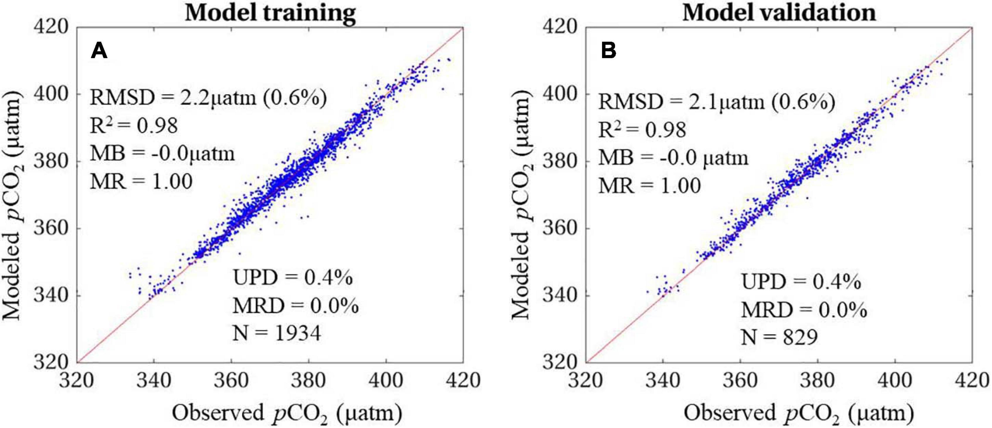
Figure 3. The RFRE model performance in estimating surface pCO₂sw in both model training (A) and model validation (B).

FIGURE 4

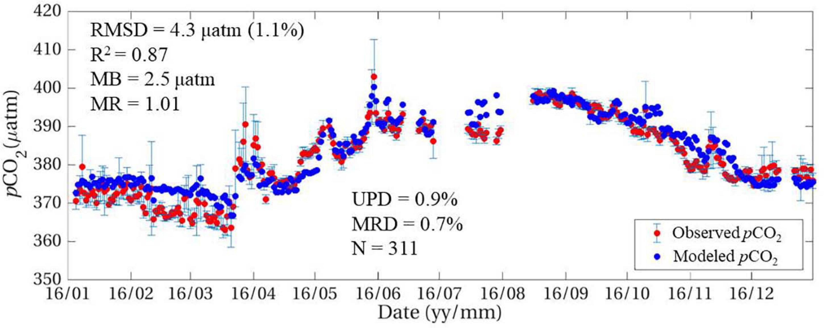
Figure 4. The RFRE model performance in reconstructing the surface pCO₂sw data time series in 2016, in comparison with the corresponding mooring-observed surface pCO₂sw. Note that none of the field observations in 2016 was used in the model development. The error bar represents one standard deviation of the diurnal changes of pCO₂sw time series.

The RFRE model is more sensitive to changes in SST and pCO₂air than to changes in Chla (Figure 5). Statistically, with + 1°C (-1°C) added to SST, the modeled pCO₂sw was higher (lower) than the original pCO₂sw, with RMSD of 9.7 μatm (2.6%) [8.0 μatm (2.1%)], R² of 0.89 (0.93), and MB of 8.5 μatm (-6.8 μatm). The resulting pCO₂sw shows slight underestimation and overestimation in cases of 20% increase and 20% decrease in Chla, with MB of 1.3 and −1.3 μatm, respectively. With + 5 μatm in pCO₂air, the new pCO₂sw was estimated higher than the original pCO₂sw, with RMSD of 5.7 μatm (1.6%), R² of 0.90, and MB of 3.7 μatm. With −5 μatm in pCO₂air, the new pCO₂sw was underestimated compared to the original pCO₂sw with RMSD of 6.1 μatm (1.6%), R² of 0.89 and MB of −4.2 μatm.

FIGURE 5

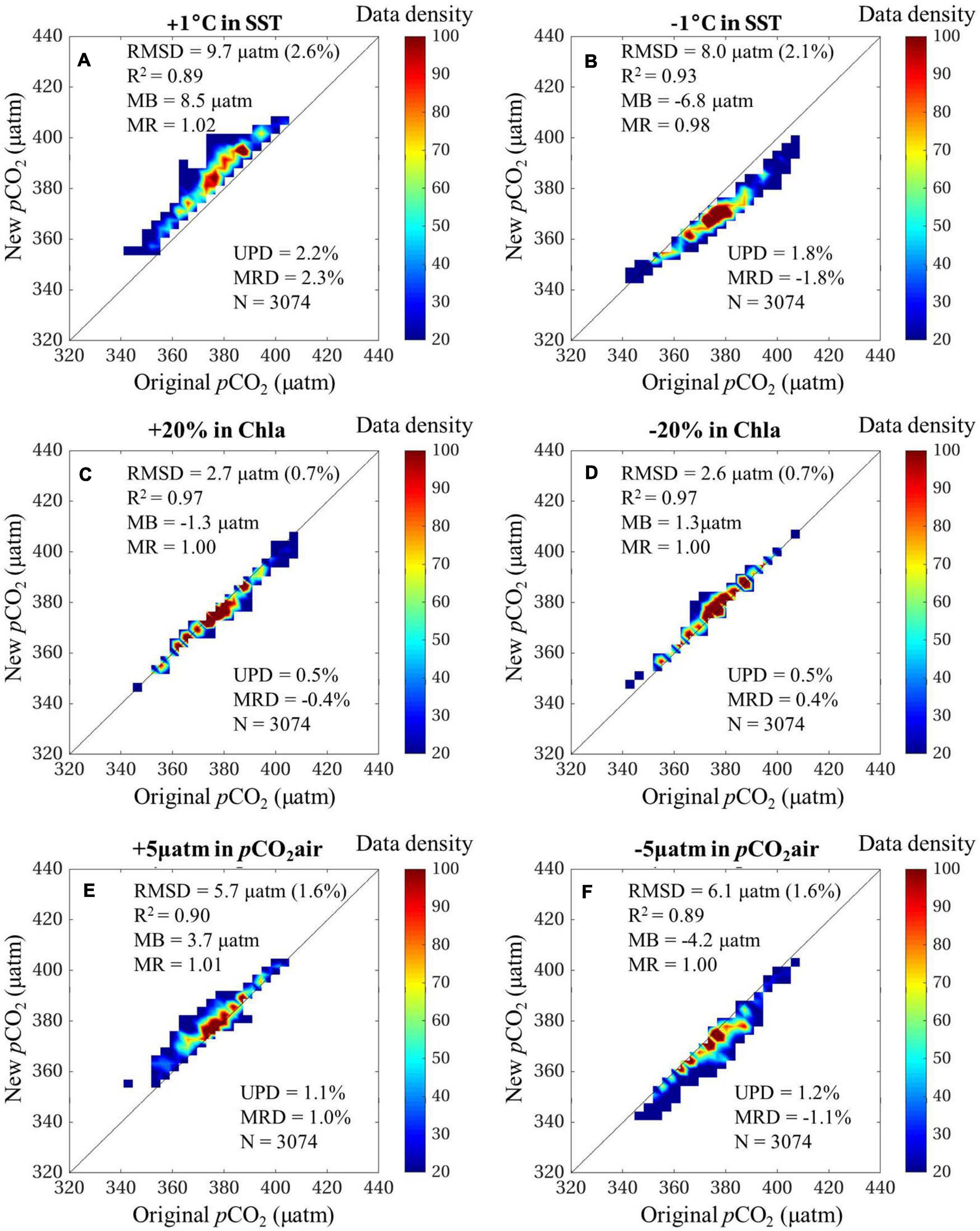
Figure 5. Sensitivity of the RFRE pCO₂sw algorithm to uncertainties in satellite-derived SST (A,B) and Chla (C,D) and to the natural variability of pCO₂air (E,F).

In the North Pacific subtropical gyre at the WHOTS station, time series of pCO₂sw between 2002 and 2019 was obtained using this RRFE-based pCO₂sw algorithm, with good consistency to the observed pCO₂sw in the overlapped time periods (Figure 6). Overall, the pCO₂sw follows the same seasonal pattern as SST from high values in summer to low values in winter, with a seasonal magnitude of ∼50 μatm, in the opposite phase of pCO₂air (Figure 6). In addition, the pCO₂sw was lower than the pCO₂air most of the time over the years, suggesting a continuous CO₂ flux from the atmosphere to the ocean.

FIGURE 6

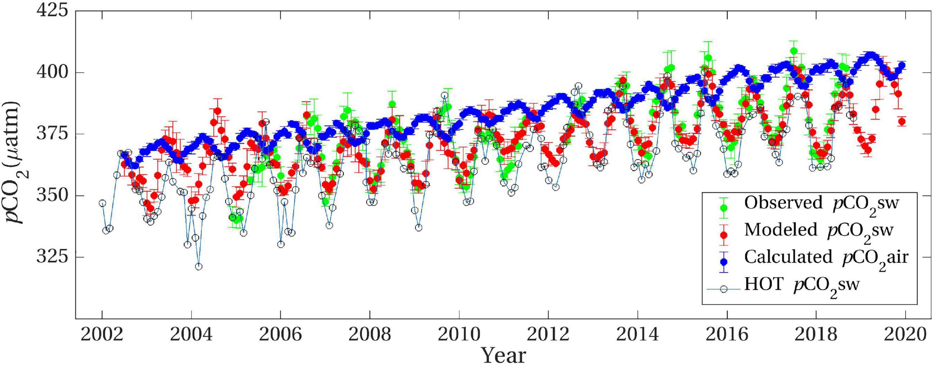
Figure 6. Modeled pCO₂sw in the full time period between 2002 and 2019, in comparison with the mooring-observed surface pCO₂sw and calculated pCO₂air at WHOTS. Note that the calculated pCO₂air is based on the data of atmospheric CO₂ measured at MLO.

Both pCO₂sw and pCO₂air show significant increase between 2002 and 2019 (Figure 6). After removing the seasonality signals, statistically, the pCO₂sw had a mean rate of 1.7 ± 0.1 μatm yr^–1 (R² = 0.80, at p < 0.05), lower than the rate of pCO₂air (2.2 ± 0.1 μatm yr^–1, R² = 0.99, at p < 0.05), as shown in Figure 7. The pCO₂sw^nat_forced shows a significant increasing rate of 0.2 ± 0.1 μatm yr^–1 (R² = 0.07, at p < 0.05) on average in the study period. In contrast, the pCO₂sw^atm_forced, which is just driven by the atmospheric CO₂ forcing, had a mean rate of 1.4 ± 0.1 μatm yr^–1 (R² = 0.84, at p < 0.05), but tended to plateau since 2016. Indeed, the pCO₂sw without the thermodynamic effect (i.e., pCO₂nonT, Chen and Hu, 2019) had similar interannual patterns as pCO_2ant at a mean rate of 1.2 ± 0.1 μatm yr^–1. Correspondingly, the Chla time series did not show any trends over the years while the SST was increasing at an overall rate of 0.03 ± 0.01°C yr^–1 (R² = 0.07, at p < 0.05). This warming trend could be influencing the pCO_2natural trend.

FIGURE 7

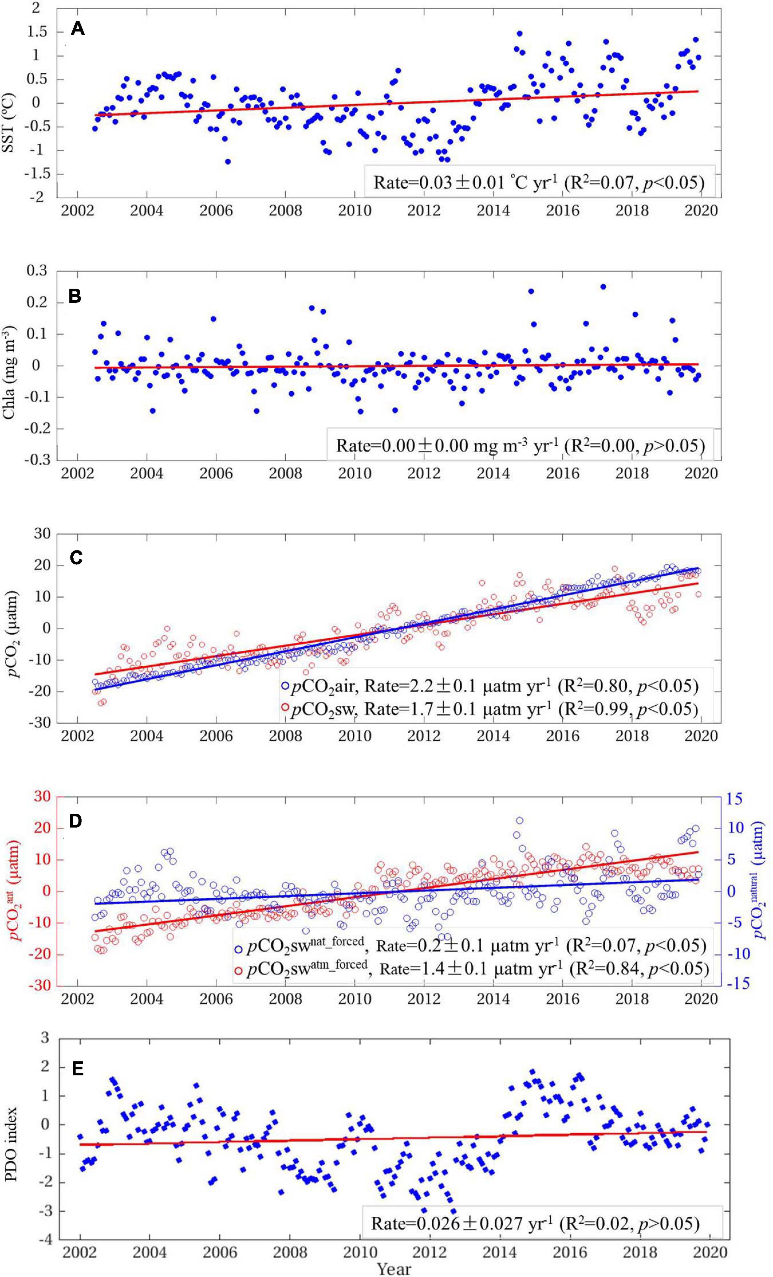
Figure 7. Interannual variations of the monthly anomalies in SST (A), Chla (B), pCO₂air and modeled pCO₂sw (C), modeled pCO₂sw^nat_forced and pCO₂sw^atm_forced (D), and PDO index (E) in the period of 2002–2019.

Clearly, there are some visible trends (e.g., <10 years) particularly in SST and pCO₂sw^nat_forced different from those over the 20-year time frame (Figure 7). To further investigate the trends in each variable, we quantified the rates of each for a variety of periods starting between 2002 and 2015, ending between 2006 and 2019, with durations ranging from 5 to 18 years (Figure 8). It is found that, at confidence level of >95%, the SST had a negative and positive rate of −0.1 ± 0.02°C yr^–1 and 0.1 ± 0.05°C yr^–1 for periods ending in ≤2013 and >2013, respectively (Figure 8A). Again, the Chla did not show any trend over the years. Correspondingly, pCO₂sw^nat_forced shows a very similar pattern as the rates in SST, with a negative rate of −0.5 ± 0.2 μatm yr^–1 for periods ending in ≤2013, and a positive rate of 0.6 ± 0.3 μatm yr^–1 for periods ending in >2013. The anthropogenic forcing on atmospheric pCO₂ tends to accelerate over the study period consistent with the published studies (Canadell et al., 2007), with a rate of 1.7 ± 0.1 μatm yr^–1 for periods ending in ≤2011, and a rate of 2.3 ± 0.2 μatm yr^–1 for periods ending in beyond 2011, and the acceleration is getting even stronger (2.4 ± 0.1 μatm yr^–1) after 2016. As a result, the pCO₂sw shows a lower rate (1.5 ± 0.4 μatm yr^–1) for periods starting in 2002–2005, ending in 2006–2019; a higher rate (2.2 ± 0.3 μatm yr^–1) for periods starting in 2006–2013, ending in 2010–2017; and a lower rate (1.5 ± 0.4 μatm yr^–1) again for periods starting in 2006–2013, ending in 2018–2019. Correspondingly, the pCO₂sw^atm_forced shows similar but significantly weaken signals (at p < 0.05) in these three time frames, with rates of 1.6 ± 0.3 μatm yr^–1, 1.8 ± 0.5μatm yr^–1, and 0.9 ± 0.5 μatm yr^–1, respectively.

FIGURE 8

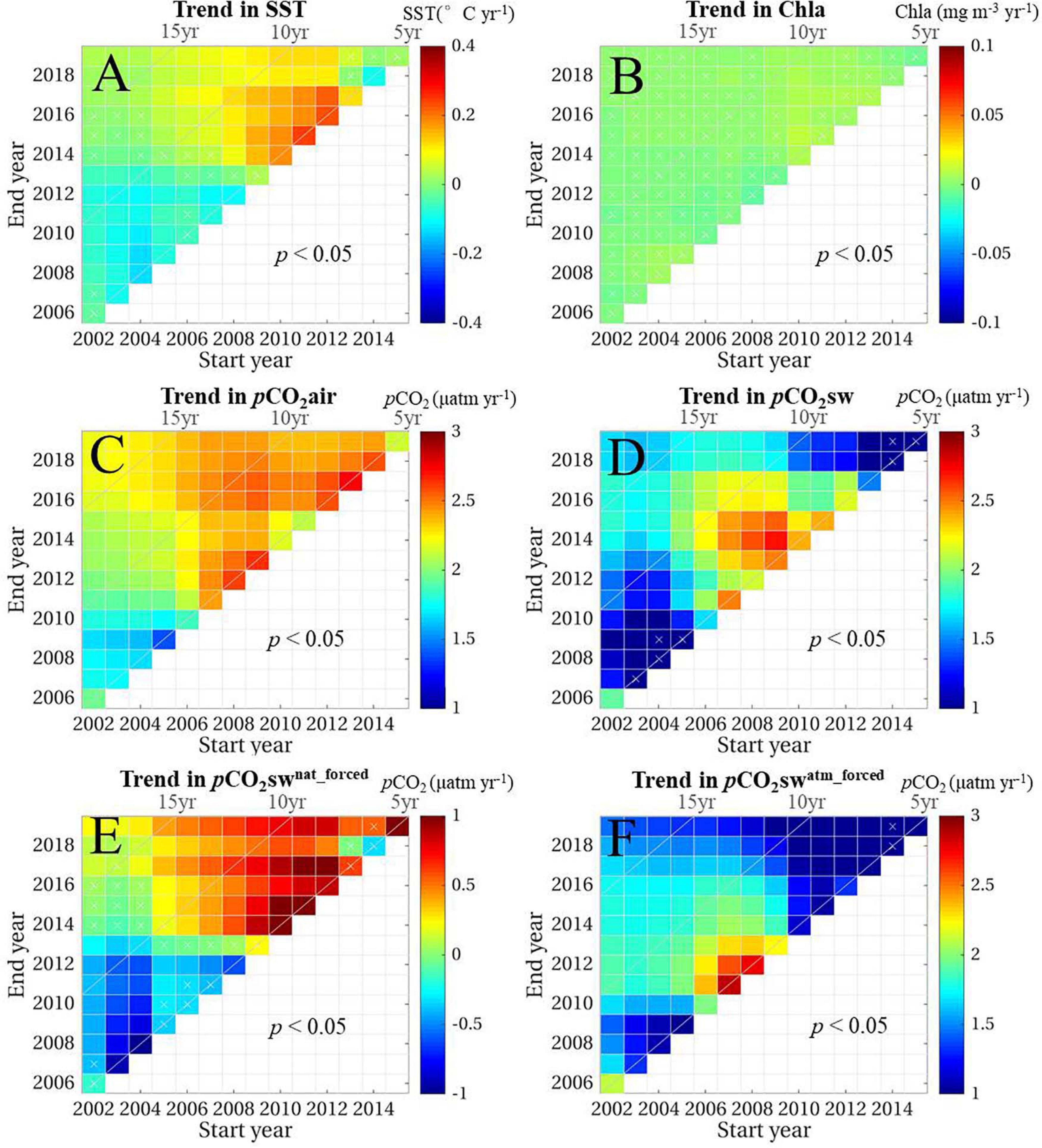
Figure 8. Interannual changing rates of SST (A), Chla (B), pCO₂air (C), modeled pCO₂sw (D), modeled pCO₂sw^nat_forced (E), and pCO₂sw^atm_forced (F) for a variety of periods starting between 2002 and 2015, and ending between 2006 and 2019 at Station WHOTS. The X-axis and Y-axis represent the start year and end year, respectively, of each rate analyzed. The diagonal lines (i.e., 5, 10, and 15 years) indicate the length of trend periods. A white cross is superposed on the plot when the p value was >0.05.

Discussion

Model Uncertainty

The satellite-based RFRE pCO₂sw model developed in this study had a RMSD of 4.3 μatm (1.1%), significantly smaller than most of the published pCO₂sw algorithms in open ocean waters (Olsen et al., 2004; Feely et al., 2006; Nakaoka et al., 2013; Moussa et al., 2016). This uncertainty is reasonably acceptable considering the diurnal variations (i.e., 0.4∼3.4 μatm) in surface pCO₂sw at WHOTS.

The sensitivity of the pCO₂sw model to each input variable indicates not only the model’s capacity in tolerating the uncertainty of each variable, but also the model’s response to real changes in each variable. Specifically, the positive feedback of modeled pCO₂sw to changes in SST are consistent with the thermodynamic effect on pCO₂sw (increased SST leads to an increase in pCO₂sw and vice versa). The negative response of the pCO₂sw model to Chla suggests that the increase (decrease) in Chla indicates stronger (weaker) biological uptake of oceanic CO₂, therefore, the resulting modeled pCO₂sw was lower (higher) than without the Chla perturbation. Although the Chla level at the WHOTS station is consistently low (Figure 2C), the sensitivity analysis here suggests the necessity of including Chla in the model to better modulate the seasonal variations of surface pCO₂sw. Yet it should be noted that, Chla is only a proxy to indicate the overall biological activities that could affect surface pCO₂sw. Although there is no visible change in surface Chla, still there could be possible changes in the phytoplankton community and net community production. The insignificant responses of the pCO₂sw model to the 20% change in Chla suggest the model is insensitive to uncertainties in the satellite Chla. For the same reason, the biological uptake of CO₂ tends to have a quite limited effect on pCO₂sw in the oligotrophic ocean, consistent with previous studies (Chen and Hu, 2019). For regions where satellite Chla is not available due to severe cloud coverage (e.g., some tropical and high latitude zones), a first examination of the Chla effect on surface pCO₂sw using field observations (if there are) is suggested to determine the potential bias that would be resulted in pCO₂sw if Chla is not included in the model. The changes of pCO₂air directly affect the gradient between pCO₂air and pCO₂sw, which drives the air-sea CO₂ exchange, thus, it is reasonable to see a positive response of the pCO₂sw model to changes in pCO₂air. The resulting increase (MB = 3.7 μatm) in pCO₂sw was slightly weaker than the assigned increase of 5 μatm in pCO₂air, which may be due to the ocean’s increasing Revelle Factor and reduced buffering capacity of seawater (Fassbender et al., 2017).

Interannual Changes of pCO₂sw Driven by Natural and Atmospheric Forcing

In response to the accelerating rates of pCO₂air, the modeled surface pCO₂sw shows different rates at various time intervals. Specifically, the 5 year pCO₂sw trends we derived for the periods of 2007–2011, 2008–2012, and 2009–2013 are high at rates of 2.5, 2.1, and 2.5 μatm yr^–1, respectively, which are higher than the relatively low rates in period of 2003–2007 visually interpreted from Figure 1 in Dore et al. (2009). To further examine the trends in pCO₂sw, we analyzed the ship-based monthly pCO₂sw datasets at ALOHA from HOT program (used in Dore et al., 2009). Indeed, the 5 year HOT-based pCO₂sw trends starting in 2007–2008 did show low values, but these low values are insignificant at p > 0.05, yet no such statistics was available in Dore et al. (2009). For the 5 year pCO₂sw trend starting in 2009, the HOT-based pCO₂sw and our modeled pCO₂sw show close trends of 2.5 and 2.2 μatm yr^–1, respectively, at p < 0.05. Meanwhile, the overall trend we detected in surface pCO₂sw (i.e., 1.7 ± 0.1μatm yr^–1) in period of 2002–2019 was a bit smaller than that (i.e., 1.88 μatm yr^–1) in period of 1988–2007 found in Dore et al. (2009) and that (i.e., 2.4 μatm yr^–1) in period of 2003–2014 presented in Sutton et al. (2017). This could be reasonable considering the different physical and biogeochemical dynamics on decadal time scales and the acceleration of ocean acidification in the western North Pacific (Ono et al., 2019). Besides, it should be noted that the ship-based monthly pCO₂sw dataset is derived from measurements of DIC and TA collected approximately once a month to compose this monthly dataset. In contrast, our monthly pCO₂sw is based on the daily modeled pCO₂sw and is validated thoroughly with daily-averaged in situ measurements at WHOTS. Therefore, the trends in the modeled pCO₂sw we derived here should be reliable with high confidence. Also, the mooring measures pCO₂sw at surface of <0.5 m, while the ship-based HOT data were based on the mean measurements within 0–30 m, which could be another potential source for the discrepancy. In the North Pacific subtropical gyre (represented by the WHOTS station), the interannual changes of surface pCO₂sw is mainly driven by both SST and pCO₂air (Figures 7, 8 and Table 1), consistent with the published studies (Takahashi et al., 2006). Despite the little impact of SSS on pCO₂sw shown in our study period (2002–2019), a further experiment with SSS added into our model was conducted. It shows that the inclusion of SSS did not result in any significant difference in the modeled pCO₂sw and pCO₂sw^nat_forced. Considering the important impact of SSS on pCO₂sw in 1989–2007 presented in Dore et al. (2003), it seems that the effect of SSS depends on the specific study periods. Here we prefer to exclude SSS from our model mainly considering the large error (i.e., 1.1) in the SMOS SSS at present. With more accurate SSS data available from satellites in the future, it could be possible to include SSS to better model the variations of pCO₂sw, particularly the effect of rainfall minus precipitation on pCO₂sw in any time periods. However, most of the published studies directly regarded the interannual trend of pCO₂sw as the trend of anthropogenic pCO₂sw. It should be noted that the anthropogenic pCO₂sw refers to the pCO₂sw impacted by atmospheric CO₂ increases, thus most of the reported anthropogenic trend of pCO₂sw actually refers to the total rate of pCO₂sw (Takahashi et al., 2009, 2014; McKinley et al., 2011; Sutton et al., 2019), which also includes the natural variability of pCO₂sw driven by the general oceanic processes (e.g., thermodynamics, ocean mixing, biological activities).

TABLE 1

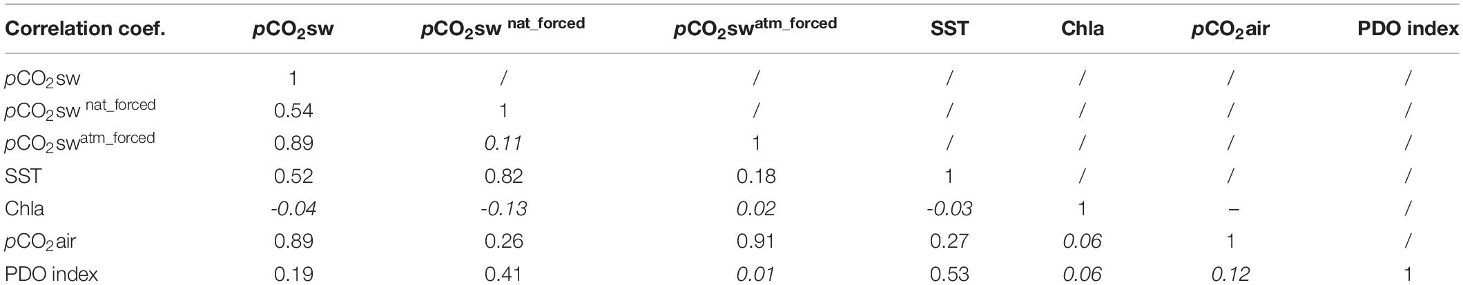
Table 1. Correlation coefficients among the monthly anomalies of pCO₂sw, pCO₂sw ^nat_forced, pCO₂sw^atm_forced, SST, Chla, pCO₂air, and PDO index, with insignificant correlation (i.e., p > 0.05) annotated in italic.

In this study, both the natural and atmospheric CO₂ forcing effects on pCO₂sw were separately quantified. The rates in pCO₂sw^nat_forced over the study period follow a similar pattern as those in SST with a correlation coefficient (R) of 0.82, indicating that the interannual trend signals in pCO₂sw^nat_forced are mainly driven by SST, at least over the study period of 2002–2019. The cooling characteristics in SST between 2002 and 2012 resulted in a significant negative rate in pCO₂sw^nat_forced, and the warming effect since 2013, which were also reported in previous studies (Sutton et al., 2017; Terlouw et al., 2019), leads to a significant positive rate in pCO₂sw^nat_forced. In addition to the global warming effect on SST, the interannual SST dynamics could also be attributed to the changes in MLD because of the ocean mixing effect on SST. As such, the interannual variations in pCO₂sw^nat_forced could also be driven by the MLD changes, and more DIC enriched waters would be entrained into the surface when MLD deepens and SST decreases (Dore et al., 2009). Overall, it seems that the rate of pCO₂sw^nat_forced tends to correspond to decadal oscillations in SST between cooling and warming periods associated with PDO (Yasunaka et al., 2014; Newman et al., 2016; Landshützer et al., 2019). Indeed, the interannual PDO (Figure 7E) shows very similar variation patterns to the SST (Figure 7A) with a significant correlation of R = 0.53 (Table 1). Specifically, the PDO decreased progressively from 2004 to 2012, was low in 2011–2012, reached a maximum in 2015, and then decreased from 2015 to 2019. As a result, the pCO₂sw^nat_forced also shows a significant correlation (R = 0.41, see Table 1) with PDO, suggesting the large scale climate forcing also contribute to the natural oceanic forcing effect on surface pCO₂sw.

With the exclusion of pCO₂sw^nat_forced, the pCO₂sw^atm_forced rates were significantly smaller than the corresponding pCO₂sw rates in various time intervals (Figure 8). Although pCO₂sw^atm_forced is mainly driven by the oceanic uptake of increasing atmospheric CO₂ (R = 0.91), it shows distinctively different patterns in changing rates from that of the pCO₂air over various time intervals in 2002–2019. This different response of pCO₂sw^atm_forced toward pCO₂air seems mainly caused by the buffering effect of dissolved CO₂ in seawater (Egleston et al., 2010). However, for the tendency of pCO₂sw^atm_forced to plateau after 2016, there could be several potential explanations depending on the condition of air-sea CO₂ fluxes. Specifically, it would be reasonable to observe a plateau signal in pCO₂sw^atm_forced if there is little change in air-sea CO₂ fluxes after 2016; yet if the dissolved CO₂ keeps increasing after 2016, the little response in pCO₂sw^atm_forced would tend to suggest that a larger fraction of dissolved CO₂ stays in forms of other carbonate species (i.e., HCO_3–, CO_32–), significantly lowering the Revelle factor and enhancing the ocean’s buffering capacity in recent years; and if there is a decrease in air-sea CO₂ fluxes after 2016, it would be likely that a fration of bicarbonate and carbonate species are converted to dissolved CO₂, which would lower the ocean’s buffering capacity and promote ocean acidification. Xue and Cai (2020) found that TA minus DIC can be used as a proxy for deciphering ocean acidification. Here using the ship-based monthly TA and DIC data in the study period, we found a significant decreasing trend in TA minus DIC over the years (Figure 9A), which suggests a strong ocean acidification in the study period. However, the changing rates of TA minus DIC is distinctively higher in recent years since 2014 (Figure 9B), suggesting a stronger ocean acidification and weaker buffering capacity in the past few years. Indeed, ocean acidification has shifted the carbonate chemistry speciation and lowered the CaCO₃ saturation state (Orr et al., 2005; Doney et al., 2009; Krug et al., 2011), yet further studies are needed to investigate and quantify the changing patterns of the air-sea CO₂ flux and the carbonate species over the past decades. In general, the oceanic uptake of anthropogenic CO₂ is resulting in more rapid changes in carbonic chemistry in the surface ocean and accelerating ocean acidification (Feely et al., 2009; Ono et al., 2019), yet a revisit of such phenomenon is needed when more satellite/field data are available in the coming years.

FIGURE 9

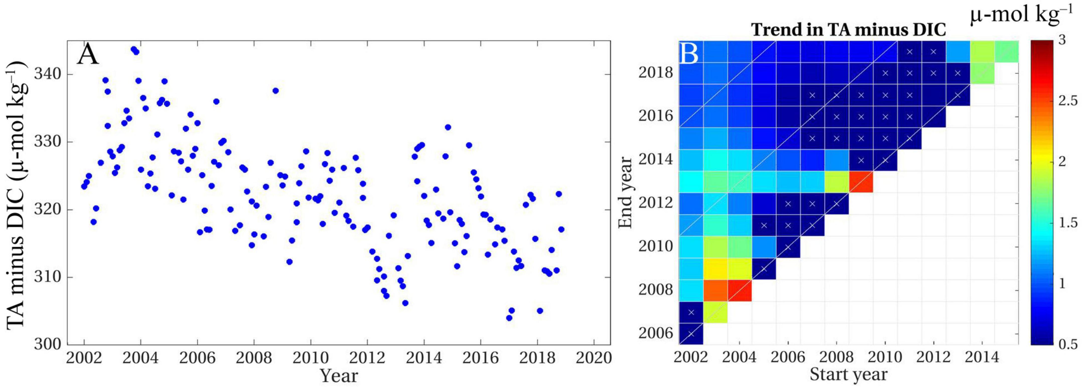
Figure 9. The interannual variations of the monthly anomalies in TA minus DIC, which was a proxy of ocean acidification, based on the ship-based monthly TA and DIC measurements at ALOHA in surface waters (A), and the corresponding interannual changing rates for a variety of periods starting between 2002 and 2015, and ending between 2006 and 2019 (B). In (B), the X-axis and Y-axis represent the start year and end year, respectively, of each rate analyzed, the diagonal lines (i.e., 5, 10, and 15 years) indicate the length of trend periods, and a white cross is superposed on the plot when the p-value was >0.05.

Implications

Long time series data are required to investigate the anthropogenic effect on surface pCO₂sw. However, the field data are always limited in both spatial and temporal coverage. For example, few of the 40 global pCO₂sw mooring stations have data coverage of >10 years (Sutton et al., 2019), and the global field pCO₂sw database (i.e., SOCAT or LDEO, Bakker et al., 2016; Takahashi et al., 2019), although greatly accumulated in recent years, still has data gaps in some regions and at some time intervals. More importantly, it is impossible or difficult to separate the pCO₂sw^atm_forced and pCO₂sw^nat_forced signals apart based on purely field measurements to better quantify the anthropogenic forcing impact on surface pCO₂sw. Instead, with the related environmental variables observed from satellites, surface pCO₂sw models using satellite data and other ancillary data can be developed and applied to the full satellite data record over the past ∼20 years. Besides, SSS measurements from SMOS and SMAP satellite have been available since 2009 and 2015, respectively, with longer and accurate data records available, the interannual and decadal trends in surface pCO₂sw as well as the natural forcing and atmospheric CO₂ forcing components can be further studied. The recovered long time series of pCO₂sw can be used to quantify both pCO₂sw^atm_forced and pCO₂sw^nat_forced accordingly. The findings of decoupled changing rates in pCO₂sw^atm_forced and pCO₂sw^nat_forced in this study highlight the necessity of differentiating the two, in order to have a better understanding of the long term oceanic absorption of anthropogenic CO₂ and its buffering capacity in the long term. Therefore, this study sets a template for future study to examine both natural and anthropogenic or atmospheric CO₂ forcing effects on pCO₂sw in various oceanic systems over the past decades, toward an improved understanding of anthropogenic forcing on surface pCO₂sw.

Specifically, the pCO₂sw in the North Pacific subtropical gyre shows various increase rates in response to the increasing pCO₂air between 2002 and 2019. The accelerating increase rates in pCO₂air and the weaker rates in pCO₂sw indicate stronger gradients between pCO₂air and pCO₂sw, which implies an accelerated oceanic CO₂ uptake and ocean acidification. If the warming effect continues following the decadal pattern in SST in recent years since 2010, a steady rate of ∼0.8 ± 0.1 μatm yr^–1 in pCO₂sw^nat_forced (see Figure 8E) would be expected in the coming few years. The weaker rate in pCO₂sw^atm_forced in recent years in response to the accelerating rate in pCO₂air implies a lower ocean buffering capacity leading to more rapidly changing oceanic carbon chemistry and ocean acidification, yet further study in this field is needed to promote our knowledge and understanding.

Based on observations at WHOTS, the present work demonstrated the necessity in differentiating the atmospheric forcing and natural forcing effects on surface pCO₂sw, and show unprecedented information on their interannual-decadal trends over both short and long time scales. The WHOTS station is located in the North Pacific Subtropical Gyre, therefore, the results and findings should be referential to understand the overall surface pCO₂sw dynamics for a broader impact of the ocean in absorbing anthropogenic CO₂, particularly under both anthropogenic CO₂ forcing and natural oceanic forcing (Henson et al., 2016).

More importantly, the pCO₂sw model was developed using satellite-derived environmental data and other ancillary data, thus the model is capable to tolerate the uncertainties involved in each variable as demonstrated in the sensitivity analysis. This is of great importance and significance to locations or areas where very limited data are available. Specifically, with these limited field observations of surface pCO₂sw, it would be possible to develop a surface pCO₂sw model with related environmental variables from satellite and ancillary data from NCEP to differentiate the two forcing effects following Eqs 1 and 2. With nearly 20 years of satellite data records, it would be straightforward to extend the current study to other oceanic regions to investigate the interannual-decadal surface pCO₂sw dynamics by differentiating the atmospheric forcing and natural forcing effects toward a better understanding of the ocean in absorbing anthropogenic CO₂ and its impact on the surface ocean carbonate chemistry.

Conclusion

The rate of anthropogenic or atmospheric CO₂ forcing pCO₂sw in surface seawater has been difficult to characterize because of the interaction of natural variability in pCO₂sw and the requirement of long time series data records. In this study, we show that a remote sensing algorithm applied to the WHOTS station in the North Pacific subtropical gyre can reveal the interannual-decadal variability of surface pCO₂sw between 2002 and 2019. Such an ability enables the separation of atmospheric CO₂ forced pCO₂sw (pCO₂sw^atm_forced) from natural variability in pCO₂sw (pCO₂sw^nat_forced). We believe that this is the first time such atmospheric CO₂ forced pCO₂sw and natural oceanic processes driven pCO₂sw are mathematically differentiated and their interannual-decadal changing rates are statistically quantified. Results show unprecedented information on their interannual-decadal rates over both short and long time scales at the WHOTS site. With the availability of ocean color data and other ancillary data globally, it is straightforward to extend the current study to other oceanic regions.

Data Availability Statement

Publicly available datasets were analyzed in this study. This data can be found here: The WHOTS mooring dataset analyzed in this study is available at National Centers for Environmental information (NCEI) under https://www.nodc.noaa.gov/ocads/oceans/Moorings/. The MODIS ocean color data are available at the NASA Goddard Space Flight Center (GSFC) https://oceancolor.gsfc.nasa.gov/. The atmospheric xCO2 data at Mauna Loa is available at the NOAA ESRL Global Monitoring Laboratory under https://www.esrl.noaa.gov/gmd/dv/data/index.php.

Author Contributions

SC designed the study, processed, analyzed the data, and wrote the manuscript. AS contributed the mooring data and main concept definition. CH and FC contributed data analysis and manuscript writing. All authors commented on the manuscript.

Funding

This work was supported by the National Natural Science Foundation of China (NSFC) projects (42030708, 41906159, and 41730536). The pCO₂ observations at WHOTS were supported by the Office of Oceanic and Atmospheric Research of the NOAA, U.S. Department of Commerce, including resources from the Global Ocean Monitoring and Observation program.

Conflict of Interest

The authors declare that the research was conducted in the absence of any commercial or financial relationships that could be construed as a potential conflict of interest.

Acknowledgments

We gratefully acknowledge the support of National Natural Science Foundation of China (NSFC) and the contribution of NOAA PMEL. The MODIS data were maintained by the NASA Goddard Space Flight Center, the daily xCO₂ data was provided by the NOAA’s Global Monitoring Laboratory. We thank NASA and NOAA for providing these data. This is PMEL contribution #5131.

Footnotes

1. ^ https://www.nodc.noaa.gov/ocads/oceans/Moorings/
2. ^ https://oceancolor.gsfc.nasa.gov/

References

Bakker, D. C., Pfeil, B., Landa, C. S., Metzl, N., O’Brien, K. M., Olsen, A., et al. (2016). A multi-decade record of high-quality fCO₂ data in version 3 of the surface ocean CO2 Atlas (SOCAT). Earth Syst. Sci. Data 8, 383–413. doi: 10.5194/essd-8-383-2016

CrossRef Full Text | Google Scholar

Bai, Y., Cai, W. J., He, X., Zhai, W., Pan, D., Dai, M., et al. (2015). A mechanistic semi-analytical method for remotely sensing sea surface pCO₂ in river-dominated coastal oceans: a case study from the East China Sea. J. Geophysical Res. Oceans 120, 2331–2349. doi: 10.1002/2014JC010632

CrossRef Full Text | Google Scholar

Barnes, B. B., and Hu, C. (2015). Cross-sensor continuity of satellite-derived water clarity in the Gulf of Mexico: insights into temporal aliasing and implications for long-term water clarity assessment. IEEE Trans. Geosci. Remote Sens. 53, 1761–1772. doi: 10.1109/TGRS.2014.2348713

CrossRef Full Text | Google Scholar

Borges, A. V., Delille, B., and Frankignoulle, M. (2005). Budgeting sinks and sources of CO₂ in the coastal ocean: diversity of ecosystems counts. Geophys. Res. Lett. 32:L14601. doi: 10.1029/2005GL023053

CrossRef Full Text | Google Scholar

Borges, A., Ruddick, K., Lacroix, G., Nechad, B., Astoreca, R., Rousseau, V., et al. (2010). Estimating pCO₂ from Remote Sensing in the Belgian Coastal Zone. Paris: ESA Special Publication, 686.

Google Scholar

Breiman, L. (1996). Bagging predictors. Mach. Learn. 24, 123–140. doi: 10.1007/BF00058655

CrossRef Full Text | Google Scholar

Breiman, L. (2001). Random forests. Mach. Learn. 45, 5–32. doi: 10.1023/A:1010933404324

CrossRef Full Text | Google Scholar

Brix, H., Gruber, N., and Keeling, C. D. (2004). Interannual variability of the upper ocean carbon cycle at station ALOHA near hawaii. Global Biogeochem. Cycles 18:GB4019. doi: 10.1029/2004GB002245

CrossRef Full Text | Google Scholar

Cai, W. J., Dai, M., and Wang, Y. (2006). Air-sea exchange of carbon dioxide in ocean margins: a province-based synthesis. Geophys. Res. Lett. 33:L12603. doi: 10.1029/2006GL026219

CrossRef Full Text | Google Scholar

Canadell, J. G., Le Quéré, C., Raupach, M. R., Field, C. B., Buitenhuis, E. T., Ciais, P., et al. (2007). Contributions to accelerating atmospheric CO2 growth from economic activity, carbon intensity, and efficiency of natural sinks. Proc. Natil. Acad. Sci. 104, 18866–18870. doi: 10.1073/pnas.0702737104

PubMed Abstract | CrossRef Full Text | Google Scholar

Chan, N. C. S., and Connolly, S. R. (2013). Sensitivity of coral calcification to ocean acidification: a meta-analysis. Global Change Biol. 19, 282–290. doi: 10.1111/gcb.12011

PubMed Abstract | CrossRef Full Text | Google Scholar

Chen, S., Hu, C., Byrne, R. H., Robbins, L. L., and Yang, B. (2016). Remote estimation of surface pCO₂ on the West Florida shelf. Cont. Shelf Res. 128, 10–25. doi: 10.1016/j.csr.2016.09.004

CrossRef Full Text | Google Scholar

Chen, S., Hu, C., Cai, W. J., and Yang, B. (2017). Estimating surface pCO₂ in the northern Gulf of Mexico: which remote sensing model to use? Cont. Shelf Res. 151, 94–110. doi: 10.1016/j.csr.2017.10.013

CrossRef Full Text | Google Scholar

Chen, S., Hu, C., Barnes, B. B., Wanninkhof, R., Cai, W. J., Barbero, L., et al. (2019). A machine learning approach to estimate surface ocean pCO2 from satellite measurements. Remote sens. Environ. 228, 203–226. doi: 10.1016/j.rse.2019.04.019

CrossRef Full Text | Google Scholar

Chen, S., and Hu, C. (2019). Environmental controls of surface water pCO₂ in different coastal environments: observations from marine buoys. Cont. Shelf Res. 183, 73–86. doi: 10.1016/j.csr.2019.06.007

CrossRef Full Text | Google Scholar

Chierici, M., Olsen, A., Johannessen, T., Trinañes, J., and Wanninkhof, R. (2009). Algorithms to estimate the carbon dioxide uptake in the northern North Atlantic using shipboard observations, satellite and ocean analysis data. Deep-Sea Res. II Top. Stud. Oceanogr. 56, 630–639. doi: 10.1016/j.dsr2.2008.12.014

CrossRef Full Text | Google Scholar

Davis, C. V., Rivest, E. B., Hill, T. M., Gaylord, B., Russell, A. D., and Sanford, E. (2017). Ocean acidification compromises a planktic calcifier with implications for global carbon cycling. Sci. Rep. 7:2225. doi: 10.1038/s41598-017-01530-9

PubMed Abstract | CrossRef Full Text | Google Scholar

Denvil-Sommer, A., Gehlen, M., Vrac, M., and Mejia, C. (2019). LSCE-FFNN-v1: a two-step neural network model for the reconstruction of surface ocean pCO 2 over the global ocean. Geosci. Model Dev. 12, 2091–2105. doi: 10.5194/gmd-12-2091-2019

CrossRef Full Text | Google Scholar

Dickinson, G. H., Ivanina, A. V., Matoo, O. B., Portner, H. O., Lannig, G., Bock, C., et al. (2012). Interactive effects of salinity and elevated CO₂ levels on juvenile eastern oysters. Crassostrea virginica. J. Exp. Biol. 215, 29–43. doi: 10.1242/jeb.061481

PubMed Abstract | CrossRef Full Text | Google Scholar

Dickson, A. G., Sabine, C. L., and Christian, J. R. (eds) (2007). Guide to Best Practices for Ocean CO₂ Measurements. Sidney: North Pacific Marine Science Organization, 176.

Google Scholar

Doney, S. C., Fabry, V. J., Feely, R. A., and Kleypas, J. A. (2009). Ocean acidification: the other CO₂ problem. Ann. Rev. Mar. Sci. 1, 169–192. doi: 10.1146/annurev.marine.010908.163834

PubMed Abstract | CrossRef Full Text | Google Scholar

Dore, J. E., Lukas, R., Sadler, D. W., and Karl, D. M. (2003). Climate-driven changes to the atmospheric CO₂ sink in the subtropical North Pacific Ocean. Nature 424, 754–757. doi: 10.1038/nature01885

PubMed Abstract | CrossRef Full Text | Google Scholar

Dore, J. E., Lukas, R., Sadler, D. W., Church, M. J., and Karl, D. M. (2009). Physical and biogeochemical modulation of ocean acidification in the central North Pacific. Proc. Natl. Acad. Sci. 106, 12235–12240. doi: 10.1073/pnas.0906044106

PubMed Abstract | CrossRef Full Text | Google Scholar

Doney, S. C. (2010). The growing human footprint on coastal and open-ocean biogeochemistry. Science 328, 1512–1516. doi: 10.1126/science.1185198

PubMed Abstract | CrossRef Full Text | Google Scholar

Egleston, E. S., Sabine, C. L., and Morel, F. M. (2010). Revelle revisited: buffer factors that quantify the response of ocean chemistry to changes in DIC and alkalinity. Global Biogeochem. Cycles 24:GB1002. doi: 10.1029/2008GB003407

CrossRef Full Text | Google Scholar

Fabricius, K. E., Langdon, C., Uthicke, S., Humphrey, C., Noonan, S., De’ath, G., et al. (2011). Losers and winners in coral reefs acclimatized to elevated carbon dioxide concentrations. Nat. Clim. Change 1, 165–169. doi: 10.1038/nclimate1122

CrossRef Full Text | Google Scholar

Fassbender, A. J., Sabine, C. L., and Palevsky, H. I. (2017). Nonuniform ocean acidification and attenuation of the ocean carbon sink. Geophys. Res. Lett. 44, 8404–8413. doi: 10.1002/2017GL074389

CrossRef Full Text | Google Scholar

Feely, R. A., Takahashi, T., Wanninkhof, R., and McPhaden, M. J. (2006). Decadal variability of the air-sea CO₂ fluxes in the equatorial Pacific Ocean. J. Geophys. Res. Oceans 111:C08S90. doi: 10.1029/2005JC003129

CrossRef Full Text | Google Scholar

Feely, R. A., Orr, J., Fabry, V. J., Kleypas, J. A., Sabine, C. L., and Langdon, C. (2009). “Present and future changes in seawater chemistry due to ocean acidification,” in Geophysical Monograph Series, eds B. J. McPherson and E. T. Sundquist (Washington, DC: American Geophysical Union), 175–188. doi: 10.1029/2005GM000337

CrossRef Full Text | Google Scholar

Fennel, K., Wilkin, J., Previdi, M., and Najjar, R. (2008). Denitrification effects on air-sea CO₂ flux in the coastal ocean: simulations for the northwest North Atlantic. Geophys. Res. Lett. 35:L24608. doi: 10.1029/2008GL036147

CrossRef Full Text | Google Scholar

Font, J., Camps, A., Borges, A., Martín-Neira, M., Boutin, J., Reul, N., et al. (2009). SMOS: the challenging sea surface salinity measurement from space. Proc. IEEE 98, 649–665. doi: 10.1109/JPROC.2009.2033096

CrossRef Full Text | Google Scholar

Font, J., Boutin, J., Reul, N., Spurgeon, P., Ballabrera-Poy, J., Chuprin, A., et al. (2013). SMOS first data analysis for sea surface salinity determination. Int. J. Remote Sens. 34, 3654–3670. doi: 10.1080/01431161.2012.716541

CrossRef Full Text | Google Scholar

Friedlingstein, P., Jones, M., O’sullivan, M., Andrew, R. M., Hauck, J., Peters, G. P., et al. (2019). Global carbon budget 2019. Earth Syst. Sci. Data 11, 1783–1838. doi: 10.5194/essd-11-1783-2019

CrossRef Full Text | Google Scholar

Friedrich, T., and Oschlies, A. (2009). Neural network-based estimates of North Atlantic surface pCO₂ from satellite data: a methodological study. J. Geophys. Res. Oceans 114:C03020. doi: 10.1029/2007JC004646

CrossRef Full Text | Google Scholar

Fujii, M., Chai, F., Shi, L., Inoue, H. Y., and Ishii, M. (2009). Seasonal and interannual variability of oceanic carbon cycling in the western and central tropical-subtropical pacific: a physical-biogeochemical modeling study. J. oceanogr. 65, 689–701. doi: 10.1007/s10872-009-0060-6

CrossRef Full Text | Google Scholar

Gregg, W. W., and Casey, N. W. (2004). Global and regional evaluation of the SeaWiFS chlorophyll data set. Remote Sens. Environ. 93, 463–479. doi: 10.1016/j.rse.2003.12.012

CrossRef Full Text | Google Scholar

Gregor, L., Lebehot, A. D., Kok, S., and Scheel Monteiro, P. M. (2019). A comparative assessment of the uncertainties of global surface ocean CO₂ estimates using a machine-learning ensemble (CSIR-ML6 version 2019a)–have we hit the wall? Geosci. Model Dev. 12, 5113–5136. doi: 10.5194/gmd-12-5113-2019

CrossRef Full Text | Google Scholar

Gruber, N., Clement, D., Carter, B. R., Feely, R. A., Van Heuven, S., Hoppema, M., et al. (2019). The oceanic sink for anthropogenic CO2 from 1994 to 2007. Science 363, 1193–1199. doi: 10.1126/science.aau5153

PubMed Abstract | CrossRef Full Text | Google Scholar

Hales, B., Strutton, P. G., Saraceno, M., Letelier, R., Takahashi, T., Feely, R., et al. (2012). Satellite-based prediction of pCO2 in coastal waters of the eastern North Pacific. Progr. Oceanogr. 103, 1–15. doi: 10.1016/j.pocean.2012.03.001

CrossRef Full Text | Google Scholar

Henson, S. A., Beaulieu, C., and Lampitt, R. (2016). Observing climate change trends in ocean biogeochemistry: when and where. Global change biol. 22, 1561–1571. doi: 10.1111/gcb.13152

PubMed Abstract | CrossRef Full Text | Google Scholar

Hu, C., Muller-Karger, F., Murch, B., Myhre, D., Taylor, J., Luerssen, R., et al. (2009). Building an automated integrated observing system to detect sea surface temperature anomaly events in the Florida keys. IEEE Trans. Geosci. Remote Sens. 47, 2071–2084. doi: 10.1109/TGRS.2009.2024992

CrossRef Full Text | Google Scholar

Iida, Y., Takatani, Y., Kojima, A., and Ishii, M. (2020). Global trends of ocean CO₂ sink and ocean acidification: an observation-based reconstruction of surface ocean inorganic carbon variables. J. Oceanogr. 77, 323–358. doi: 10.1007/s10872-020-00571-5

CrossRef Full Text | Google Scholar

Ikawa, H., Faloona, I., Kochendorfer, J., Paw, U., and Oechel, W. C. (2013). Air–sea exchange of CO₂ at a Northern California coastal site along the california current upwelling system. Biogeosciences 10, 4419–4432. doi: 10.5194/bg-10-4419-2013

CrossRef Full Text | Google Scholar

James, G., Witten, D., Hastie, T., and Tibshirani, R. (2013). Tree-Based Methods, an Introduction to Statistical Learning, Vol. 112. New York, NY: Springer, 303–328. doi: 10.1007/978-1-4614-7138-7_8

CrossRef Full Text | Google Scholar

Jo, Y. H., Dai, M., Zhai, W., Yan, X. H., and Shang, S. (2012). On the variations of sea surface pCO₂ in the northern South China Sea: a remote sensing based neural network approach. J. Geophys. Res. Oceans 117:C08022. doi: 10.1029/2011JC007745

CrossRef Full Text | Google Scholar

Karl, D. M., and Church, M. J. (2018). Station ALOHA: a gathering place for discovery, education, and scientific collaboration. Limnol. Oceanogr. Bull. 28, 10–12. doi: 10.1002/lob.10285

CrossRef Full Text | Google Scholar

Keeling, C. D., Brix, H., and Gruber, N. (2004). Seasonal and long−term dynamics of the upper ocean carbon cycle at station ALOHA near hawaii. Global Biogeochem. Cycles 18:GB4006. doi: 10.1029/2004GB002227

CrossRef Full Text | Google Scholar

Krug, S., Schulz, K., and Riebesell, U. (2011). Effects of changes in carbonate chemistry speciation on Coccolithus braarudii: a discussion of coccolithophorid sensitivities. Biogeosciences (BG) 8, 771–777. doi: 10.5194/bg-8-771-2011

CrossRef Full Text | Google Scholar

Landshützer, P., Gruber, N., Bakker, D. C. E., Schuster, U., Nakaoka, S., Payne, M. R., et al. (2013). A neural network-based estimate of the seasonal to inter-annual variability of the Atlantic Ocean carbon sink. Biogeosciences 10, 7793–7815. doi: 10.5194/bg-10-7793-2013

CrossRef Full Text | Google Scholar

Landshützer, P., Gruber, N., and Bakker, D. C. (2016). Decadal variations and trends of the global ocean carbon sink. Global Biogeochem. Cycles 30, 1396–1417. doi: 10.1002/2015GB005359

CrossRef Full Text | Google Scholar

Landshützer, P., Ilyina, T., and Lovenduski, N. S. (2019). Detecting regional modes of variability in observation−based surface ocean pCO₂. Geophys. Res. Lett. 46, 2670–2679. doi: 10.1029/2018GL081756

CrossRef Full Text | Google Scholar

Le, C., Gao, Y., Cai, W. J., Lehrter, J. C., Bai, Y., and Jiang, Z. P. (2019). Estimating summer sea surface pCO2 on a river-dominated continental shelf using a satellite-based semi-mechanistic model. Remote Sens. Environ. 225, 115–126. doi: 10.1016/j.rse.2019.02.023

CrossRef Full Text | Google Scholar

Lee, K., Choi, S. D., Park, G. H., Wanninkhof, R., Peng, T. H., Key, R. M., et al. (2003). An updated anthropogenic CO₂ inventory in the Atlantic Ocean. Global Biogeochem. Cycles 17:1116. doi: 10.1029/2003GB002067

CrossRef Full Text | Google Scholar

Lefèvre, N., Watson, A. J., and Watson, A. R. (2005). A comparison of multiple regression and neural network techniques for mapping in situ pCO₂ data. Tellus B 57, 375–384. doi: 10.1111/j.1600-0889.2005.00164.x

CrossRef Full Text | Google Scholar

Lohrenz, S. E., and Cai, W. J. (2006). Satellite ocean color assessment of air-sea fluxes of CO₂ in a river-dominated coastal margin. Geophys. Res. Lett. 33, L01601. doi: 10.1029/2005GL023942

CrossRef Full Text | Google Scholar

Lohrenz, S. E., Cai, W. J., Chen, F., Chen, X., and Tuel, M. (2010). Seasonal variability in air-sea fluxes of CO₂ in a river-influenced coastal margin. J. Geophys. Res. Oceans 115:C10034. doi: 10.1029/2009JC005608

CrossRef Full Text | Google Scholar

Lohrenz, S. E., Cai, W. J., Chakraborty, S., Huang, W. J., Guo, X., He, R., et al. (2018). Satellite estimation of coastal pCO₂ and air-sea flux of carbon dioxide in the northern Gulf of Mexico. Remote Sens. Environ. 207, 71–83. doi: 10.1016/j.rse.2017.12.039

CrossRef Full Text | Google Scholar

Lukas, R., and Santiago-Mandujano, F. (2008). Interannual to interdecadal salinity variations observed near hawaii: local and remote forcing by surface freshwater fluxes. Oceanography 21, 46–55. doi: 10.5670/oceanog.2008.66

CrossRef Full Text | Google Scholar

Marrec, P., Cariou, T., Macé, É, Morin, P., Salt, L. A., Vernet, M., et al. (2015). Dynamics of air-sea CO 2 fluxes in the northwestern European shelf based on voluntary observing ship and satellite observations. Biogeosciences 12, 5371–5391. doi: 10.5194/bg-12-5371-2015

CrossRef Full Text | Google Scholar

McKinley, G. A., Fay, A. R., Takahashi, T., and Metzl, N. (2011). Convergence of atmospheric and North Atlantic carbon dioxide trends on multidecadal timescales. Nat. Geosci. 4, 606–610. doi: 10.1038/ngeo1193

CrossRef Full Text | Google Scholar

Mélin, F., Zibordi, G., and Berthon, J. F. (2007). Assessment of satellite ocean color products at a coastal site. Remote Sens. Environ. 110, 192–215. doi: 10.1016/j.rse.2007.02.026

CrossRef Full Text | Google Scholar

Moussa, H., Benallal, M. A., Goyet, C., and Lefèvre, N. (2016). Satellite-derived CO₂ fugacity in surface seawater of the tropical Atlantic Ocean using a feedforward neural network. Int. J. Remote Sens. 37, 580–598. doi: 10.1080/01431161.2015.1131872

CrossRef Full Text | Google Scholar

Nakaoka, S., Telszewski, M., Nojiri, Y., Yasunaka, S., Miyazaki, C., Mukai, H., et al. (2013). Estimating temporal and spatial variation of ocean surface pCO₂ in the North Pacific using a self-organizing map neural network technique. Biogeosciences 10, 6093–6106. doi: 10.5194/bg-10-6093-2013

CrossRef Full Text | Google Scholar

Newman, M., Alexander, M. A., Ault, T. R., Cobb, K. M., Deser, C., Di Lorenzo, E., et al. (2016). The pacific decadal oscillation, revisited. J Clim. 29, 4399–4427. doi: 10.1175/JCLI-D-15-0508.1

CrossRef Full Text | Google Scholar

NOAA ESRL Global Monitoring Laboratory (2019). “updated annually.” in Atmospheric Carbon Dioxide Dry Air Mole Fractions from Quasi-Continuous Measurements at Mauna Loa, Hawaii, Barrow, Alaska, American Samoa and South Pole, Version 2020-04. eds K. W. Thoning, A. Crotwell, and D. R. Kitzis (Boulder, CO: National Oceanic and Atmospheric Administration),Google Scholar

Olsen, A., Triñanes, J. A., and Wanninkhof, R. (2004). Sea–air flux of CO₂ in the caribbean sea estimated using in situ and remote sensing data. Remote Sens. Environ. 89, 309–325. doi: 10.1016/j.rse.2003.10.011

CrossRef Full Text | Google Scholar

Ono, T., Saino, T., Kurita, N., and Sasaki, K. (2004). Basin-scale extrapolation of shipboard pCO₂ data by using satellite SST and Chl a. Int. J. Remote Sens. 25, 3803–3815. doi: 10.1080/01431160310001657515

CrossRef Full Text | Google Scholar

Ono, T., Kosugi, N., Toyama, K., Tsujino, H., Kojima, A., Enyo, K., et al. (2019). Acceleration of Ocean Acidification in the Western North Pacific. Geophys. Res. Lett. 46, 13161–13169. doi: 10.1029/2019GL085121

CrossRef Full Text | Google Scholar

Orr, J. C., Fabry, V. J., Aumont, O., Bopp, L., Doney, S. C., Feely, R. A., et al. (2005). Anthropogenic ocean acidification over the twenty-first century and its impact on calcifying organisms. Nature 437, 681–686. doi: 10.1038/nature04095

PubMed Abstract | CrossRef Full Text | Google Scholar

Palevsky, H. I., and Quay, P. D. (2017). Influence of biological carbon export on ocean carbon uptake over the annual cycle across the North Pacific ocean. Global Biogeochem. Cycles 31, 81–95. doi: 10.1002/2016GB005527

CrossRef Full Text | Google Scholar

Parard, G., Charantonis, A. A., and Rutgerson, A. (2015). Remote sensing the sea surface CO₂ of the Baltic Sea using the SOMLO methodology. Biogeosciences 12, 3369–3384. doi: 10.5194/bg-12-3369-2015

CrossRef Full Text | Google Scholar

Quay, P., Sonnerup, R., Munro, D., and Sweeney, C. (2017). Anthropogenic CO₂ accumulation and uptake rates in the Pacific Ocean based on changes in the ¹³C/¹²C of dissolved inorganic carbon. Global Biogeochem. Cycles 31, 59–80. doi: 10.1002/2016GB005460

CrossRef Full Text | Google Scholar

Rayner, N. A. A., Parker, D. E., Horton, E. B., Folland, C. K., Alexander, L. V., Rowell, D. P., et al. (2003). Global analyses of sea surface temperature, sea ice, and night marine air temperature since the late nineteenth century. J. Geophys. Res. Atmos. 108:4407. doi: 10.1029/2002JD002670

CrossRef Full Text | Google Scholar

Rödenbeck, C., Bakker, D. C., Gruber, N., Iida, Y., Jacobson, A. R., Jones, S., et al. (2015). Data-based estimates of the ocean carbon sink variability–first results of the Surface Ocean pCO₂ mapping intercomparison (SOCOM). Biogeosciences 12, 7251–7278. doi: 10.5194/bg-12-7251-2015

CrossRef Full Text | Google Scholar

Sabine, C. L., Feely, R. A., Key, R. M., Bullister, J. L., Millero, F. J., Lee, K., et al. (2002). Distribution of anthropogenic CO₂ in the Pacific Ocean. Global Biogeochem. Cycles 16, 30–31. doi: 10.1029/2001GB001639

CrossRef Full Text | Google Scholar

Sabine, C. L., Feely, R. A., Gruber, N., Key, R. M., Lee, K., Bullister, J. L., et al. (2004a). The oceanic sink for anthropogenic CO₂. Science 305, 367–371. doi: 10.1126/science.1097403

PubMed Abstract | CrossRef Full Text | Google Scholar

Sabine, C. L., Feely, R. A., Watanabe, Y. W., and Lamb, M. (2004b). Temporal evolution of the North Pacific CO₂ uptake rate. J. Oceanogr. 60, 5–15. doi: 10.1023/B:JOCE.0000038315.23875.ae

CrossRef Full Text | Google Scholar

Sabine, C., Sutton, A., McCabe, K., Lawrence-Slavas, N., Alin, S., Feely, R., et al. (2020). Evaluation of a new carbon dioxide system for autonomous surface vehicles. J. Atmos. Ocean. Technol. 37, 1305–1317. doi: 10.1175/JTECH-D-20-0010.1

CrossRef Full Text | Google Scholar

Sarma, V. V. S. S., Saino, T., Sasaoka, K., Nojiri, Y., Ono, T., Ishii, M., et al. (2006). Basin-scale pCO₂ distribution using satellite sea surface temperature, Chl a, and climatological salinity in the North Pacific in spring and summer. Glob. Biogeochem. Cycles 20: GB3005. doi: 10.1029/2005GB002594

CrossRef Full Text | Google Scholar

Signorini, S. R., Mannino, A., Najjar, R. G., Friedrichs, M. A., Cai, W. J., Salisbury, J., et al. (2013). Surface ocean pCO₂ seasonality and sea-air CO₂ flux estimates for the North American east coast. J. Geophys. Res. Oceans 118, 5439–5460. doi: 10.1002/jgrc.20369

CrossRef Full Text | Google Scholar

Shadwick, E. H., Thomas, H., Comeau, A., Craig, S. E., Hunt, C. W., and Salisbury, J. E. (2010). Air-Sea CO₂ fluxes on the scotian shelf: seasonal to multi-annual variability. Biogeosciences 7, 3851–3867. doi: 10.5194/bg-7-3851-2010

CrossRef Full Text | Google Scholar

Sutton, A. J., Sabine, C. L., Dietrich, C., Maenner Jones, S., Musielewicz, S., Bott, R., et al. (2012). High-Resolution Ocean and Atmosphere Pco₂ Time-Series Measurements From Mooring Whots_158w_23n North Pacific Ocean (Ncei Accession 0100080). [Data in 2004-2017]. Washington, D.C: NOAA, doi: 10.3334/CDIAC/otg.TSM_WHOTS

CrossRef Full Text | Google Scholar

Sutton, A. J., Sabine, C. L., Maenner-Jones, S., Lawrence-Slavas, N., Meinig, C., Feely, R. A., et al. (2014). A high-frequency atmospheric and seawater pCO₂ data set from 14 open-ocean sites using a moored autonomous system. Earth Syst. Sci. Data 6, 353–366. doi: 10.5194/essd-6-353-2014

CrossRef Full Text | Google Scholar

Sutton, A. J., Wanninkhof, R., Sabine, C. L., Feely, R. A., Cronin, M. F., and Weller, R. A. (2017). Variability and trends in surface seawater pCO₂ and CO₂ flux in the Pacific Ocean. Geophys. Res. Lett. 44, 5627–5636. doi: 10.1002/2017GL073814

CrossRef Full Text | Google Scholar

Sutton, A. J., Feely, R. A., Maenner-Jones, S., Musielwicz, S., Osborne, J., Dietrich, C., et al. (2019). Autonomous seawater pCO₂ and pH time series from 40 surface buoys and the emergence of anthropogenic trends. Earth System Sci. Data 11, 421–439. doi: 10.5194/essd-11-421-2019

CrossRef Full Text | Google Scholar

Takahashi, T., Sutherland, S. C., Feely, R. A., and Wanninkhof, R. (2006). Decadal change of the surface water pCO₂ in the North Pacific: a synthesis of 35 years of observations. J. Geophys. Res. Oceans 111:C07S05. doi: 10.1029/2005JC003074

CrossRef Full Text | Google Scholar

Takahashi, T., Sutherland, S. C., Wanninkhof, R., Sweeney, C., Feely, R. A., and Baar, H. (2009). Climatological mean and decadal change in surface ocean pCO2, and net sea–air CO₂ flux over the global oceans. Deep Sea Res. II Top. Stud. Oceanogr. 56, 554–577. doi: 10.1016/j.dsr2.2008.12.009

CrossRef Full Text | Google Scholar

Takahashi, T., Sutherland, S. C., Chipman, D. W., Goddard, J. G., Ho, C., Newberger, T., et al. (2014). Climatological distributions of pH, pCO₂, total CO₂, alkalinity, and CaCO₃ saturation in the global surface ocean, and temporal changes at selected locations. Mar. Chem. 164, 95–125. doi: 10.1016/j.marchem.2014.06.004

CrossRef Full Text | Google Scholar

Takahashi, T., Sutherland, S. C., and Kozyr, A. (2019). Global Ocean Surface Water Partial Pressure of CO2 Database: Measurements Performed During 1957-2018 (LDEO Database Version 2018) (NCEI Accession 0160492). Version 7.7. Washington, D.C: NOAA, Google Scholar

Tao, Z., Qin, B., Li, Z., and Yang, X. (2012). Satellite observations of the partial pressure of carbon dioxide in the surface water of the huanghai sea and the bohai sea. Acta Oceanol. Sin. 31, 67–73. doi: 10.1007/s13131-012-0207-y

CrossRef Full Text | Google Scholar

Terlouw, G. J., Knor, L. A., De Carlo, E. H., Drupp, P. S., Mackenzie, F. T., Li, Y. H., et al. (2019). Hawaii coastal seawater CO₂ network: a statistical evaluation of a decade of observations on tropical coral reefs. Front. Mar. Sci. 6:226. doi: 10.3389/fmars.2019.00226

CrossRef Full Text | Google Scholar

Wanninkhof, R., Park, G. H., Takahashi, T., Sweeney, C., Feely, R. A., Nojiri, Y., et al. (2013). Global ocean carbon uptake: magnitude. Variability Trends.Biogeosci. 10, 1983–2000. doi: 10.5194/bg-10-1983-2013

CrossRef Full Text | Google Scholar

Weiss, R. F. (1974). Carbon dioxide in water and seawater: the solubility of a non-ideal gas. Mar. Chem. 2, 203–215. doi: 10.1016/0304-4203(74)90015-2

CrossRef Full Text | Google Scholar

Widdicombe, S., and Spicer, J. I. (2008). Predicting the impact of ocean acidification on benthic biodiversity: what can animal physiology tell us? J. Exp. Mar. Biol. Ecol. 366, 187–197. doi: 10.1016/j.jembe.2008.07.024

CrossRef Full Text | Google Scholar

Xiu, P., and Chai, F. (2014). Variability of oceanic carbon cycle in the North Pacific from seasonal to decadal scales. J. Geophys. Res. Oceans 119, 5270–5288. doi: 10.1002/2013JC009505

CrossRef Full Text | Google Scholar

Xue, L., Cai, W. J., Hu, X., Sabine, C., Jones, S., Sutton, A. J., et al. (2016). Sea surface carbon dioxide at the Georgia time series site (2006–2007): air–sea flux and controlling processes. Prog. Oceanogr. 140, 14–26. doi: 10.1016/j.pocean.2015.09.008

CrossRef Full Text | Google Scholar

Xue, L., and Cai, W. J. (2020). Total alkalinity minus dissolved inorganic carbon as a proxy for deciphering ocean acidification mechanisms. Mar. Chem. 222:103791. doi: 10.1016/j.marchem.2020.103791

CrossRef Full Text | Google Scholar

Yasunaka, S., Nojiri, Y., Nakaoka, S. I., Ono, T., Mukai, H., and Usui, N. (2014). North Pacific dissolved inorganic carbon variations related to the Pacific decadal oscillation. Geophys. Res. Lett. 41, 1005–1011. doi: 10.1002/2013GL058987

CrossRef Full Text | Google Scholar

Zhu, Y., Shang, S., Zhai, W., and Dai, M. (2009). Satellite-derived surface water pCO₂ and air–sea CO₂ fluxes in the northern South China sea in summer. Prog. Nat. Sci. 19, 775–779. doi: 10.1016/j.pnsc.2008.09.004

CrossRef Full Text | Google Scholar