 Eileen H. Bates1*
 Lindsay Alma1
 Tamas Ugrai2
 Alexander Gagnon2Michael Maher3
 Paul McElhany3
 Jacqueline L. Padilla-Gamiño1
- 1School of Aquatic and Fishery Sciences, University of Washington, Seattle, WA, United States
- 2School of Oceanography, University of Washington, Seattle, WA, United States
- 3National Oceanic and Atmospheric Administration (NOAA), Northwest Fisheries Science Center Mukilteo Research Station, Mukilteo, WA, United States
Global climate change is causing ocean acidification (OA), warming, and decreased dissolved oxygen (DO) in coastal areas, which can cause physiological stress and compromise the health of marine organisms. While there is increased focus on how these stressors will affect marine species, there is little known regarding how changes in water chemistry will impact the bioaccumulation of trace metals. This study compared trace metal concentrations in tissue of Mediterranean mussels (Mytilus galloprovincialis) and Olympia oysters (Ostrea lurida) in Puget Sound, Washington, a region that experiences naturally low pH, seasonal hypoxia, and is surrounded by urbanized and industrialized areas. Shellfish were held at three sites (Carr Inlet, Point Wells, and Dabob Bay) where oceanographic data was continuously collected using mooring buoys. Using inductively coupled plasma mass-spectrometry (ICP-MS) to measure trace metals in the tissue, we found differences in accumulation of trace metals based on species, location, and shellfish size. Our study found differences between sites in both the mean metal concentrations and variability around the mean of those concentrations in bivalves. However, high metal concentrations in bivalves were not associated with high concentrations of metals in seawater. Metal concentrations in shellfish were associated with size: smaller shellfish had higher concentrations of metals. Carr Inlet at 20 m depth had the smallest shellfish and the highest metal concentrations. While we could not eliminate possible confounding factors, we also found higher metal concentrations in shellfish associated with lower pH, lower temperature, and lower dissolved oxygen (conditions seen at Carr Inlet at 20 m and to a lesser extent at Point Wells at 5 m depth). There were also significant differences in accumulation of metals between oysters and mussels, most notably copper and zinc, which were found in higher concentrations in oysters. These findings increase our understanding of spatial differences in trace metal bioaccumulation in shellfish from Puget Sound. Our results can help inform the Puget Sound aquaculture industry how shellfish may be impacted at different sites as climate change progresses and coastal pollution increases.
Introduction
Climate change poses a global threat, but will particularly impact coastal areas such as marginal seas through both land and marine driven changes in precipitation, runoff, sea level rise, ocean circulation, and seawater chemistry (Scavia et al., 2002; Harley et al., 2006; Pachauri et al., 2014). As global climate change continues, marine species will face increasing seawater temperatures, continued ocean acidification, and lower dissolved oxygen availability (Pachauri et al., 2014). Coastal cities and areas with high river discharge will also face the threat of increased pollution (Fowler and Oregioni, 1976; Wang et al., 2018), which may have important consequences for bioaccumulation of metals and chemicals in marine organisms, further impacting their physiology and survival.
In marginal seas such as Puget Sound, research has been conducted on the variation of pH, temperature, and DO in coastal zones and how these oceanographic variables may interact to affect physiological performance, reproduction, and survival of species (Handisyde et al., 2006; Washington Sea Grant, 2015; Gobler and Baumann, 2016). To date, however, the indirect effects of water chemistry changes on the accumulation of trace metals in Puget Sound shellfish—a critical intersection of pollution and climate change— has been overlooked.
Changes in seawater pH, temperature, and DO can affect the solubility and speciation of metals, which in turn can affect their bioavailability and their impact on cellular processes of marine organisms (Millero, 2001; Millero et al., 2009; Smith et al., 2015). Aquatic chemistry models have demonstrated that the speciation of metals that are strongly hydrolyzed in seawater (including Al3+, Cr3+, Fe3+) and those dominated by carbonate complexation (including Cu cations) appear to be more heavily influenced by changes in temperature and pH. In contrast, metals that are weakly complexed in seawater (including Mn2+, Fe2+, Co2+, Ni2+, and Zn2+), and those dominated by chloride complexation (including Cu+, Cd2+) appear less influenced by temperature and pH changes (Byrne et al., 1988). Smith et al. (2015) used a biotic ligand model to predict the toxicity of various metals based on chemical speciation. To date, however, there is limited direct observational data on many of these chemical speciation models, adding a degree of uncertainty to the results they predict and increasing the need for more direct, field-based studies, especially in biological contexts (Byrne et al., 1988). Further, chemical speciation alone cannot always be used to predict metal uptake in organisms, because uptake can vary with species, life stage, metal biochemistry, and CO2 levels in the water (Götze et al., 2014; Ivanina and Sokolova, 2015; Sezer et al., 2020). These limitations emphasize the importance of collecting empirical data in furthering our understanding of how trace metal accumulation will vary in space and time as temperature and pCO2 increase due to anthropogenic effects.
Our study uses field experiments to better understand how the trace metal accumulation of shellfish in Puget Sound, Washington, United States will be altered in a changing climate. The Puget Sound region has over 4.8 million inhabitants (United States Census Bureau, 2020) and is seeing the effects of anthropogenic climate change earlier than many other regions of the global ocean. Waters in Puget Sound already have naturally low pH from upwelling of deep seawater rich in CO2 (Feely et al., 2010, 2012), which in conjunction with anthropogenic CO2 inputs makes the water in this region especially corrosive for shellfish and other calcifiers. In addition, areas of Puget Sound are already seasonally hypoxic, which will only worsen with increased anthropogenic climate change and eutrophication (Keister and Tuttle, 2013). Shellfish aquaculture is a very important industry in this region; Washington state is the largest producer of farmed clams, oysters, and mussels in the United States, and the economic contribution of the industry in 2011 was estimated at $270 million (Washington Sea Grant, 2015). Oyster farmers on the west coast have already felt the effects of high CO2 through production failures in oyster aquaculture in the early 2000s (Mabardy et al., 2015).
In addition to their economic value, shellfish such as bivalves are commonly used to monitor and determine toxicity and pollution in coastal areas. In the Mediterranean Sea and the Bohai Sea, studies have found that metal concentrations in mollusks vary with site, and concentrations are correlated with proximity to highly populated areas and industries such as zinc, gold smelting, and paper mills (Fowler and Oregioni, 1976; Wang et al., 2005). In addition to spatial variation in accumulation, studies in Spain, Scotland, and Tasmania have found that bivalves accumulate higher levels of metals than other phyla (Topping, 1972; Eustace, 1974; Olmedo et al., 2013). There are also differences in accumulation between shellfish species: off the coast of China, oysters accumulated metals such as copper, zinc, and cadmium more readily than mussels (Wang et al., 2018). In Brazil, oysters, as rapid filterers, have been found to be a useful metric for monitoring trace metal pollution levels in estuarine sediments at sites with varying proximity to human impact (Wanick et al., 2012), and in a study comparing clams and oysters, elevated CO2 levels had a greater impact on accumulation of copper and cadmium in oysters than in clams (Hawkins and Sokolova, 2017).
Studies conducted on accumulation of specific trace metals in shellfish under ocean acidification scenarios have produced varying and sometimes contradictory results. Short-term hypercapnia (excessive CO2 in bloodstream) in clams increased copper uptake but suppressed cadmium uptake in mantle tissue (Ivanina et al., 2013). In another study, low pH (pH ∼ 7.8 and 7.4, compared to control pH ∼ 8.1) resulted in higher cadmium concentrations after a 30 day experiment on two species of clams and one species of mussel (Shi et al., 2016). Interestingly, Millero et al. (2009) noted that the speciation of cadmium should not change considerably with shifts in pH, perhaps indicating that differences in cadmium accumulation seen in experiments were not necessarily due to speciation changes. A multi-stressor study on the shell and tissue accumulation of metals in the oyster C. gigas found temperature to have a greater impact than pH on accumulation of several metals including cadmium, manganese, and cobalt (Belivermiş et al., 2016). In cuttlefish, though, accumulation of cadmium and manganese was found to decrease with pH (Lacoue-Labarthe et al., 2012). These inconsistent results underscore the need for further studies on trace metal accumulation under ecologically relevant conditions.
To best prepare for the effects of future climate change and coastal population growth, we require a better understanding of how environmental changes will influence the availability of trace metals and how this may affect marine organisms and the humans who rely on them as a food source. Some metals (e.g., iron, copper, zinc, and manganese), are necessary for biological processes, but can be toxic at higher concentrations (Sivaperumal et al., 2007; Millero et al., 2009; Olmedo et al., 2013; Chan and Wang, 2018). Other metals (e.g., cadmium, mercury, and lead) are toxic even at low levels (Sivaperumal et al., 2007). Metal accumulation and toxicity have occurred in experiments using ocean acidification and temperature changes at levels that are expected under climate change scenarios (Ivanina et al., 2016; Hawkins and Sokolova, 2017; Nardi et al., 2017; Cao et al., 2018, 2019). Detrimental metal accumulation in shellfish can affect immune functions or result in oxidative stress, affecting lipids, proteins, and DNA, which in turn impact growth and reproduction and can cause pathological conditions (Ivanina et al., 2016; Chan and Wang, 2018; Wang et al., 2018).
In Puget Sound, previous research found that heavy metals such as lead, arsenic, and cadmium had the highest concentrations in urban bays such as Commencement Bay near Tacoma and Elliott Bay near Seattle (Long, 1982). In Elliott Bay, particulate copper and zinc were distributed throughout the bay, while dissolved copper and zinc levels were associated with shoreline anthropogenic sources. One study that focused on effluent from Seattle wastewater treatments found that the effluent did not significantly increase the water and biota concentrations of nickel, copper, zinc, and cadmium (Schell and Nevissi, 1977). Sediment cores have revealed that efforts to mitigate point sources of metal pollutants have been relatively effective—for example the closing of a metal smelter in Tacoma, WA decreased arsenic pollution. However, as the population around Puget Sound grows, non-point sources of pollutants, which are harder to track, will become more important to consider (Brandenberger et al., 2008). This collection of research leaves unanswered questions about the current condition of trace metal accumulation in Puget Sound particularly as the effects of climate change intensify. Areas of coastal upwelling and oxygen minimum zones—characteristics of the Puget Sound region—will be informative areas in which to learn how future climate change will impact metal speciation and complexation (Millero et al., 2009).
This project aimed to determine if concentrations of trace metals in the tissue of oysters (Ostrea lurida) and mussels (Mytilus galloprovincialis) vary with site and associated environmental variables across Puget Sound. We hypothesized that we would see differences in trace metal accumulation between species and sites, and that relative similarities between sites may be linked to the presence of similar water chemistry properties between sites. We also hypothesized that variability in pH, dissolved oxygen, and temperature at each site would have different impacts on metal accumulation, and these effects would be unique for each metal.
Materials and Methods
Study Sites and Oceanographic Data Collection
Hatchery raised shellfish were used for the experiment. Approximately 1-year-old Olympia oysters (Ostrea lurida) (Figure 1A) were acquired from Puget Sound Restoration Fund (average length 17.51 mm ± 2.41 mm) and 1-year-old Mediterranean mussels (Mytilus galloprovincialis) (Figure 1B) were acquired from Taylor Shellfish Farms (average length 28.17 mm ± 4.01 mm). Shellfish were deployed at three sites in mesh bags within cages in the water column for 1 year (Dabob Bay: deployed 7/13/2018, midpoint collection 1/15/2019, final collection 7/11/2019; Carr Inlet: deployed 7/12/2019, midpoint collection 1/8/2019, final collection 7/18/2019; Point Wells: deployed 7/13/2019, midpoint collection 1/23/2019, final collection 7/23/2019). At Dabob Bay (47.803° N, 122.803° W) and Point Wells (47.761° N, 122.397° W), shellfish cages were hung at 5 m depth (DB5 and PW5), and at Carr Inlet (47.28° N, 122.728° W), shellfish cages were hung at both 5 m and 20 m depths (CI5 and CI20) (Figure 1C). The water depth was approximately 47 m at Carr Inlet, and approximately 100 m at both Dabob Bay and Point Wells, so shellfish did not interact directly with substrate. The deployment sites were located at three ORCA (Oceanic Remote Chemical Analyzer) buoys, operated by the University of Washington Applied Physics Laboratory (APL), which allowed environmental data to be continuously collected for each site at the appropriate depths (Figure 1D). Dissolved oxygen, temperature, salinity, pH, and chlorophyll data was collected every 6 h throughout the water column and made available online through the Northwest Association of Networked Ocean Observing Systems (NANOOS). Data were used from 12:00 pm and 12:00 am each day (plus or minus 2 h when the buoy measurements did not exactly line up). When sensors on the buoys malfunctioned or did not record during the course of the study, data from the Live Ocean Model at the cage-specific depths were used instead (MacCready et al., 2020). The Live Ocean Model has been extensively validated and produces reliable results for the region. Dissolved oxygen measurements from the buoys that read negative numbers were also replaced with model data. Sensor malfunctions resulted in model data being used for 36.6% of temperature and 37.9% of DO data from CI 20 m, 36.5% of temperature and 37.8% of DO data from CI 5 m, 31.7% of temperature and 37.1% of DO data from PW 5 m, and 81.8% of temperature and 81.8% of DO data from DB 5 m.
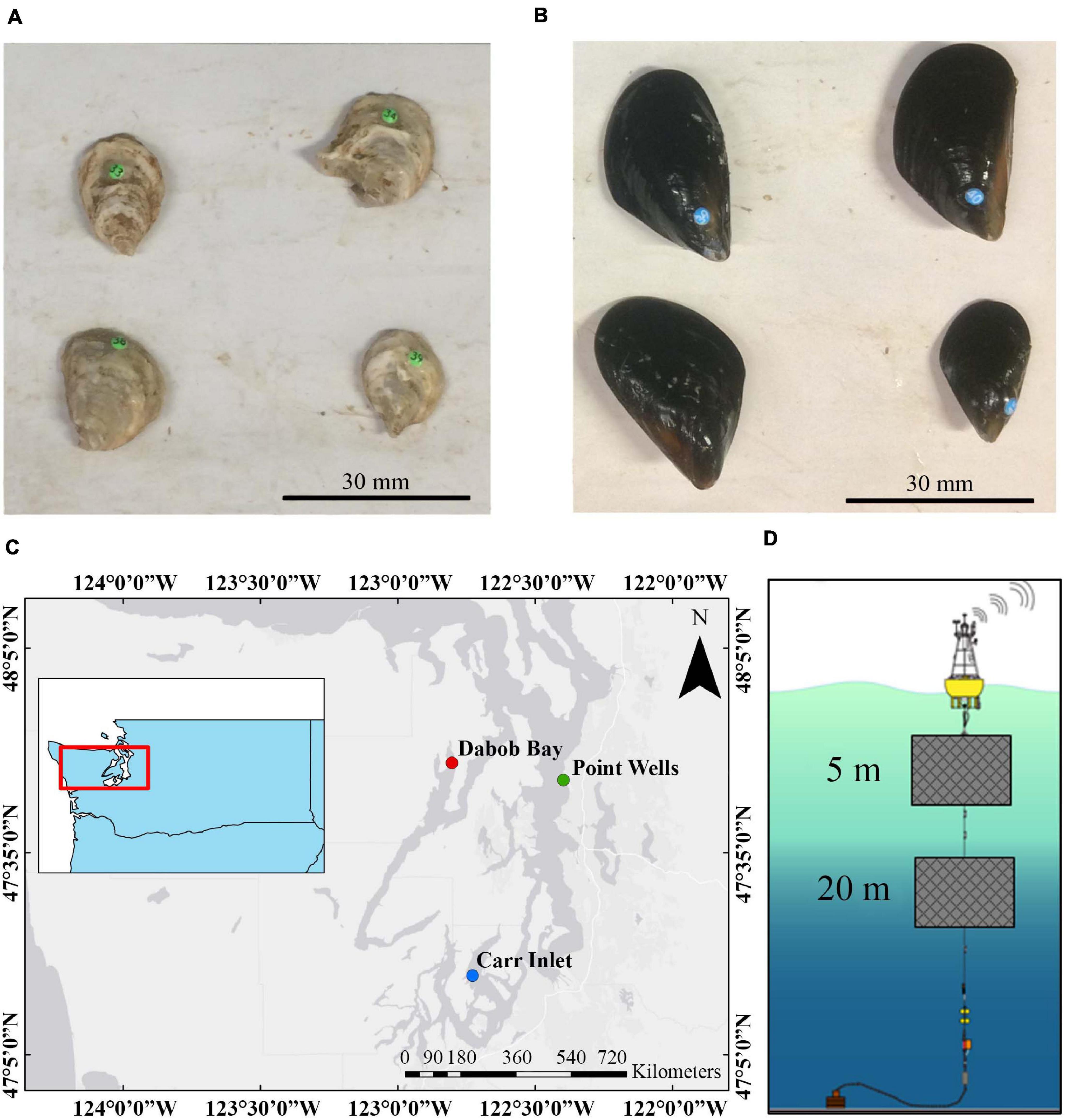
Figure 1. (A) Photograph of oysters in June 2018. (B) Photograph of mussels in June 2018. (C) Map of Puget Sound showing the locations of ORCA buoys where shellfish were deployed. Oysters and mussels were deployed at Dabob Bay (Hood Canal) at 5 m depth, Point Wells (central Puget Sound) at 5 m depth, and Carr Inlet (south Puget Sound) at both 5 m and 20 m depths. (D) A diagram of how shellfish were deployed below ORCA buoys in the field. Diagram adapted from Northwest Environmental Moorings group, Applied Physics Laboratory, University of Washington.
Trace Metal Analysis
Shellfish were dissected with ceramic knives to remove tissue from shells. Each individual was bagged, flash frozen, and kept at −80°C until future analysis. Ten oysters and ten mussels were preserved from each cage at each of the two time points (160 shellfish total). When analysis began, each specimen was transferred to a 50 mL Environmental Express digestion tube which was previously acid leached and rinsed several times in 18 MΩ water to eliminate the possibility of trace metal contamination. Shellfish samples were freeze dried at approximately −90°C and 60–80 mtor for ∼ 48 h, at which point dry weight was taken.
Shellfish samples were digested in acid and hydrogen peroxide to break down organic matter into liquid samples that could be processed with the ICP-MS (Inductively Coupled Plasma Mass Spectrometer). Samples were randomly sorted into 10 groups of 16 tubes (five groups for the January field samples and five groups from the July field samples) for acid digestions. Acid digestion was adapted from two established methods (Environmental Protection Agency, 1996; Ashoka et al., 2009). Samples were heated by a graphite hot block at ∼ 95°C in 10 mL of 1:1 HNO3:H2O, and three aliquots of 2 mL HNO3 (Fisher Scientific, trace metal grade) were added 30 min apart. A final aliquot of 1 mL H2O2 (Fisher Scientific, ACS certified) was added. Samples were then kept on the hot block until liquid had evaporated to 10–12 mL, at which point the samples were allowed to cool, and the tubes filled to 50 mL with 18 MΩ water. The samples were then diluted 10× into 10 mL sample tubes and were analyzed using an iCAP RQ ICP-MS at the University of Washington Trace Lab. Calibration curves containing 10 ppt, 100 ppt, 1 ppb, 10 ppb, 50 ppb, and 100 ppb of a multielement standard from High Purity Standards were analyzed along with the samples. For Mg, a final standard of 500 ppb was also used in the calibration curves. Four USGS metal standards (T-221, T-231, T-235, and T-239), analyzed in duplicate, were run as a secondary calibration verification. The analysis provided the concentrations of Mg, Al, Ca, Ti, Cr, Mn, Fe, Co, Ni, Cu, Zn, As, and Cd, in each sample. An internal standard solution containing Rh was added continuously to the sample stream during ICP-MS analysis to correct for instrument drift via an apparatus similar to a T-mixer.
Data Reduction
Output from the ICP-MS was provided in counts per second. Sample values were corrected based on the signal of the internal standard (Rh) and values from calibration blanks and digest blanks were subtracted from sample values. Then sample metal concentrations were determined using the slope of the calibration curve and values for metal concentration were normalized to dry weight (mmol metal/g dry tissue). For metals that had ICP-MS data collected for multiple isotopes, the isotope with the better recoveries in the USGS standards were used in analysis. Ti showed poor or inconsistent recoveries for all isotopes and was excluded from the study.
Standards and Quality Control for Trace Metal Analysis
To ensure consistency and allow for data validation, several quality control measures were used. During each of the 10 batches of acid digestions, the following 8 standards were run along with the 16 samples: 2 digestion blanks, where the same additions of HNO3 and H2O2 were performed in the hot block, but no tissue was included; 1 spiked digestion blank, which had 2 ppb of trace metal standard added to the empty tube immediately before digestion; 2 samples of DOLT-5 dogfish liver certified reference material for trace metals and other constituents from NRCC (National Research Council Canada) that also underwent acid digestion; 2 mussel standards, which were freeze dried and blended together to form a uniform powder which was distributed into 2 samples in each of the digestions used as a consistency standard; and 1 spiked mussel standard, which went through the same process but was spiked with 2 ppb of trace metals after freeze-drying but before digestion, consistent with other studies using similar methodology (Waidmann et al., 1994; Weldegebriel et al., 2012; Schmidt et al., 2013).
Seawater Sample Analysis
Water samples from each study site (5 m at Dabob Bay and Point Wells, and 5 m and 20 m for Carr Inlet) were collected in July 2018 and January 2019. Samples were collected using SCUBA from appropriate depths in Nalgene bottles that had been previously acid leached and rinsed several times in 18 MΩ water to eliminate the possibility of trace metal contamination and filled with 18 MΩ water to avoid air compression during diving. Half of the seawater samples were filtered in an all-plastic filter apparatus using 0.2 μm Millipore filters that had been previously acid leached. All seawater samples were then acidified to a pH less than 2 using ultra pure HCl (Optima). Acidification of filtered samples preserves dissolved metals in solution by limiting precipitation and loss of samples to the container sidewalls, while acidification of unfiltered samples preserves the total metals in particulate and dissolved matter. Trace metals in these seawater samples were then separated from matrix ions like Na+ and Cl- using a seaFAST automated preconcentration system (ESI). The concentrated metal samples and processed calibration standards were then analyzed using an Element 2 High-Resolution ICP-MS at the University of Washington Trace Lab. For quality control purposes an analytical duplicate and matrix spike were also processed every 10 samples on the seaFAST and then analyzed on the Element. Separate internal standards added prior to preconcentration and just prior to ICP-MS analysis were used to account for any differences in column recovery or ICP-MS stability during analysis. This analysis provided data for six elements in seawater: Fe, Co, Ni, Cu, Zn, and Cd.
Data Analysis
All statistical analyses were conducted in R version 4.0.1.
Four tissue samples from the July field collection were removed from the data set due to spills or overflows during the tissue digestion process. Although none of these samples were multivariate outliers, the possibility of lost sample during preparation was sufficient reason to remove them from both multivariate and univariate analyses.
To assess how the levels of individual metals in oyster and mussel tissue related to the metal concentrations in the associated seawater samples (filtered and unfiltered), we used simple linear regression (metals in tissue ∼ metals in seawater) and used the associated adjusted R2 and p-values to determine the significance of those relationships. Trace metals in the seawater samples taken in July 2018 and January 2019 were compared to the tissue samples collected in July 2019 and January 2019, respectively. Although the July water and tissue sampling were 1 year apart due to difficulties in sample collection, we elected to include the comparison, as water conditions were relatively similar between July 2018 and 2019 (Figure 2). The comparison between shellfish tissue, which reflects continuous metal accumulation over time, and water samples, which reflect point measurements, is imperfect. However, we felt the presentation of available seawater trace metal data was important, as it is difficult to collect and therefore less frequently available. A Bonferroni correction was applied to the original alpha value of 0.05 because the regression was being repeated six times for the six metals analyzed in seawater, so the corrected alpha level used was 0.0083 to reduce the likelihood of Type I error.
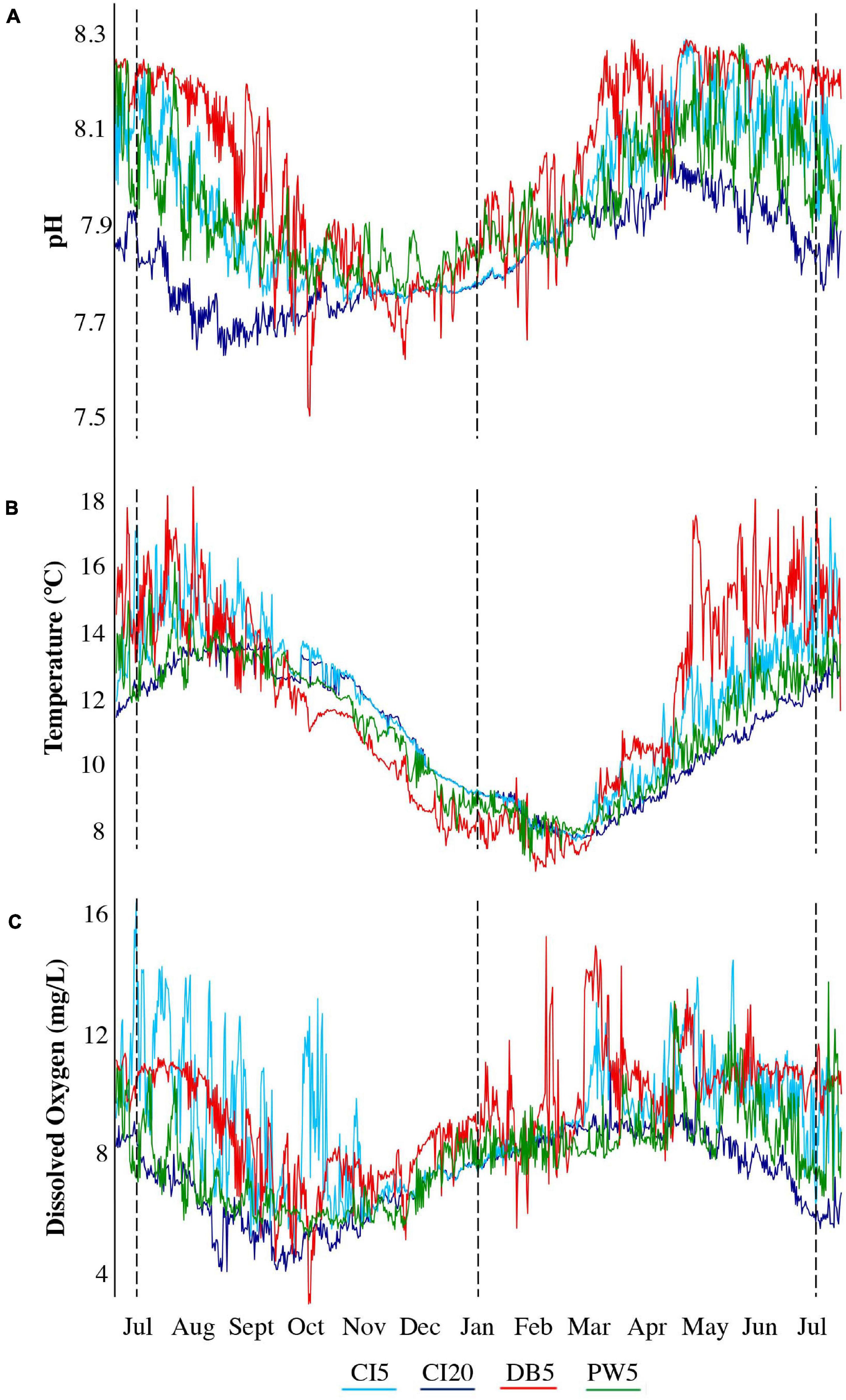
Figure 2. Environmental data at the four shellfish cage locations from July 2018– July 2019 for (A) pH calculated using TIC and Alkalinity from Live Ocean Model data, (B) temperature (combination of ORCA buoy and Live Ocean Model Data), and (C) dissolved oxygen (combination of ORCA buoy and Live Ocean Model Data). Dotted vertical lines indicate approximately when the shellfish were deployed (July 2018), when the first shellfish samples were taken (January 2019), and when the final shellfish samples were taken (July 2019).
In order to test the hypothesis that the overall metal accumulation would differ between species and sampling time, the Adonis function was used to perform perMANOVA using a Euclidean distance matrix on the cube root transformed data (Oksanen et al., 2016). Accumulation of the 12 metals was compared between the two species and the two sampling times. An alpha level of 0.05 was chosen. Concentrations of the twelve metals individually were also compared between mussels and oysters using t-tests. A Bonferroni correction was again applied to account for 12 repeated t-tests, resulting in an alpha level of 0.004.
Principal component analysis (PCA) was performed on correlation matrices (to mitigate differences in scale between concentrations of different trace metals) of the oyster and mussel data to evaluate whether accumulation of certain metals was correlated and whether there were patterns of metal accumulation based on treatment or location (Husson et al., 2013; Kassambara and Mundt, 2017). The broken-stick model (Jackson, 1993) was used to determine if eigenvalues for each principle component were greater than would be expected by chance (the broken-stick expectation), and therefore considered to represent a statistically significant fraction of the original variation in the data. Eigenvector coefficients (variable loadings) were converted into Pearson product-moment correlations and these structure coefficients represented the correlation between the original variables and each of the principal component scores. Biplots were created to visualize the location of samples and magnitude of variable importance in ordination space. We screened for multivariate outliers in the data sets for the PCA. Although several data points were more than three standard deviations from the mean of average distances (using Euclidean distance), we did not exclude these data points.
In addition to multivariate analyses on the metals in aggregate, we also wanted to assess the effects of location on individual metal levels. In order to determine which dependent variables (metals) were impacted by season at each site, one-way ANOVAs and Tukey Post-Hoc tests were run for each metal to compare differences in metal concentrations between the four locations at the two time points (treated as 8 distinct groups) for each of the two species (Huberty and Morris, 1989). While this produced results for every pair of season-specific locations, only those comparing the same location across seasons were included. Again, a Bonferroni correction was applied because the ANOVA was being repeated 12 times for the 12 metals, so the corrected alpha level used was 0.004. To assess the difference in metal accumulation between sites within each sampling period, ANOVA and Tukey Post-Hoc Tests were again run, this time for the mussel and oyster data separately for January and July, again with an alpha value of 0.004 after a Bonferroni correction.
To assess how the size of the shellfish affected the accumulation of trace metals, we again performed regression, this time exponential (metals in tissue ∼ ln(sample dry weight)), and used adjusted R2 and p-values from that regression to determine significance of these relationships. After a Bonferroni correction was used to account for repeated regressions for the 12 metals, the alpha level was 0.004.
Toxicity and Consumption Estimates
Various available metrics (adequate daily intake, average daily intake, upper level of intake per day, and maximum level permitted) were found for each of the analyzed metals (Table 1). There was no single regulating agency with metrics available for all metals, and no upper suggested limits on consumption exist for certain metals, which is why a variety of metrics were used. To estimate how intake of metals from consuming Puget Sound shellfish compared to these regulated levels, concentration of metals in wet shellfish tissue samples was estimated by multiplying the concentration of metal in dried samples by 0.22 (the average dry to wet weight ratio for the January samples). Using molecular weight and assuming 227 g (0.5 lb) daily consumption, the daily level of metals consumed was calculated for mussels and oysters from each site to be compared to regulated levels.
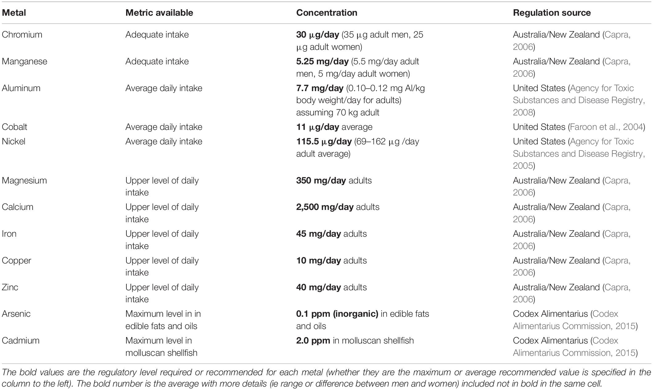
Table 1. Regulations/recommendations for metal intake for adult humans for Cr, Mn, Al, Co, Ni, Mg, Ca, Fe, Cu, and Zn, and the maximum concentrations allowed in shellfish for As (inorganic) and Cd.
Results
Quality Control
As samples were processed in two batches using ICP-MS, controls were compared between those two runs. Supplementary Table 1 summarizes the recoveries for the four USGS standards from each run. Supplementary Table 2 summarizes the recoveries of the DOLT-5 standard reference material, replicates of which were included in each tissue digestion and were processed with the ICP-MS in the same batch as the corresponding digestion group. For the USGS standards, recoveries were lower for the July field data than for the January field data. The lower percent recovery may mean that some metals are underestimated in the July samples by 10s of percent, but this does not affect our conclusions when comparing metal accumulation at different sites or between different species (Supplementary Table 1). For the DOLT-5 standard reference material, the average recoveries for the ICP-MS runs for the January data and the July data were within 10% of each other, with the exception of Mg, where the July data had a lower average recovery. All DOLT-5 samples showed a relatively lower percent recovery than the USGS standards, which means there is either some consistent loss in all samples (which would not change patterns we find for metals) or that the dry weight normalization in the dogfish is different in some way from our shellfish samples (Supplementary Table 2). This is not unheard of, as Ashoka et al. (2009) found upon comparing digestion methods that multiple digestion techniques show low recoveries for certain elements, and that no one method produced the best recoveries across all targeted elements for the different sample types they tested.
Environmental Data
All three sites (at 5 m) showed lower pH values in the late fall and early winter months (Figure 2A). Carr Inlet 20 m consistently had the lowest pH throughout the year, with minimum pH values in late summer. Throughout the year Dabob Bay 5 m showed the highest pH values, Carr Inlet 5 m the second highest, and Point Wells 5 m the third highest. Dabob Bay showed the greatest fluctuations in pH, with a few peaks well below the minimum level at any other site (Supplementary Figure 1A). From July 2018 through July 2019, at Carr Inlet 20 m, the minimum and maximum pH were 7.63 and 8.12; for Carr Inlet 5 m: 7.68 and 8.29, for Point Wells 5 m: 7.75 and 8.28, and for Dabob Bay 5 m: 7.50 and 8.29. The mean pH values for the sites were 7.83 (CI 20 m), 7.95 (CI 5 m), 7.94 (PW 5 m), and 8.03 (DB 5 m) (Figure 2A).
Minimum temperatures at all sites were found in February and March, while maximum temperatures were found in July and August (Figure 2B). Dabob Bay 5 m showed the greatest variability in temperature especially during the summer months. For Carr Inlet 20 m, the minimum and maximum temperature were: 7.84 and 13.90°C; for Carr Inlet 5 m: 7.73 and 17.47°C; for Point Wells 5 m: 7.17 and 16.15°C; and for Dabob Bay 5 m: 6.86 and 18.74°C. The mean temperatures were 11.00 (CI 20 m), 11.82°C (CI 5 m), 11.17 (PW 5 m), and 11.89°C (DB 5 m) (Figure 2B and Supplementary Figure 1B).
For dissolved oxygen, the minimum and maximum values for Carr Inlet 20 m were 4.01 and 10.98 mg/L, for Carr Inlet 5 m were 4.80 and 16.40 mg/L; for Point Wells 5 m were 5.07 and 13.74 mg/L; and for Dabob Bay 5 m were 2.92 and 15.27 mg/L. The mean DO values were 7.20 mg/L (CI 20 m), 9.10 mg/L (CI 5 m), 7.81 mg/L (PW 5 m), and 9.35 mg/L (DB 5 m) (Figure 2C). Carr Inlet 20 m showed less variability compared to the 5 m sites. High variability in dissolved oxygen occurred from spring through fall at Carr Inlet 5 m, winter through mid-summer for Dabob Bay 5 m, and just in late spring and summer for Point Wells 5 m (Figure 2C and Supplementary Figure 1C).
Trace Metal Seawater Analysis
Comparing filtered to unfiltered samples should allow determination of what fraction of metals were dissolved in the seawater as opposed to in particulate matter. There is a trend across all six metals analyzed in seawater that the unfiltered water samples had higher concentrations of metals than the filtered samples. Fe, Co, Zn, and Cu showed particularly large differences between filtered and unfiltered seawater, though lack of replicate water samples prevent statistical analyses. Largest seasonal changes for unfiltered metals were seen for Fe and Zn, with higher concentrations in January than July. Larger differences in trace metals abundance were found between seasons than between sites. Notable exceptions include lower levels of Zn at Carr Inlet 20 m in January and higher levels of Fe and Co at Carr Inlet 5 m in January (Figure 3).
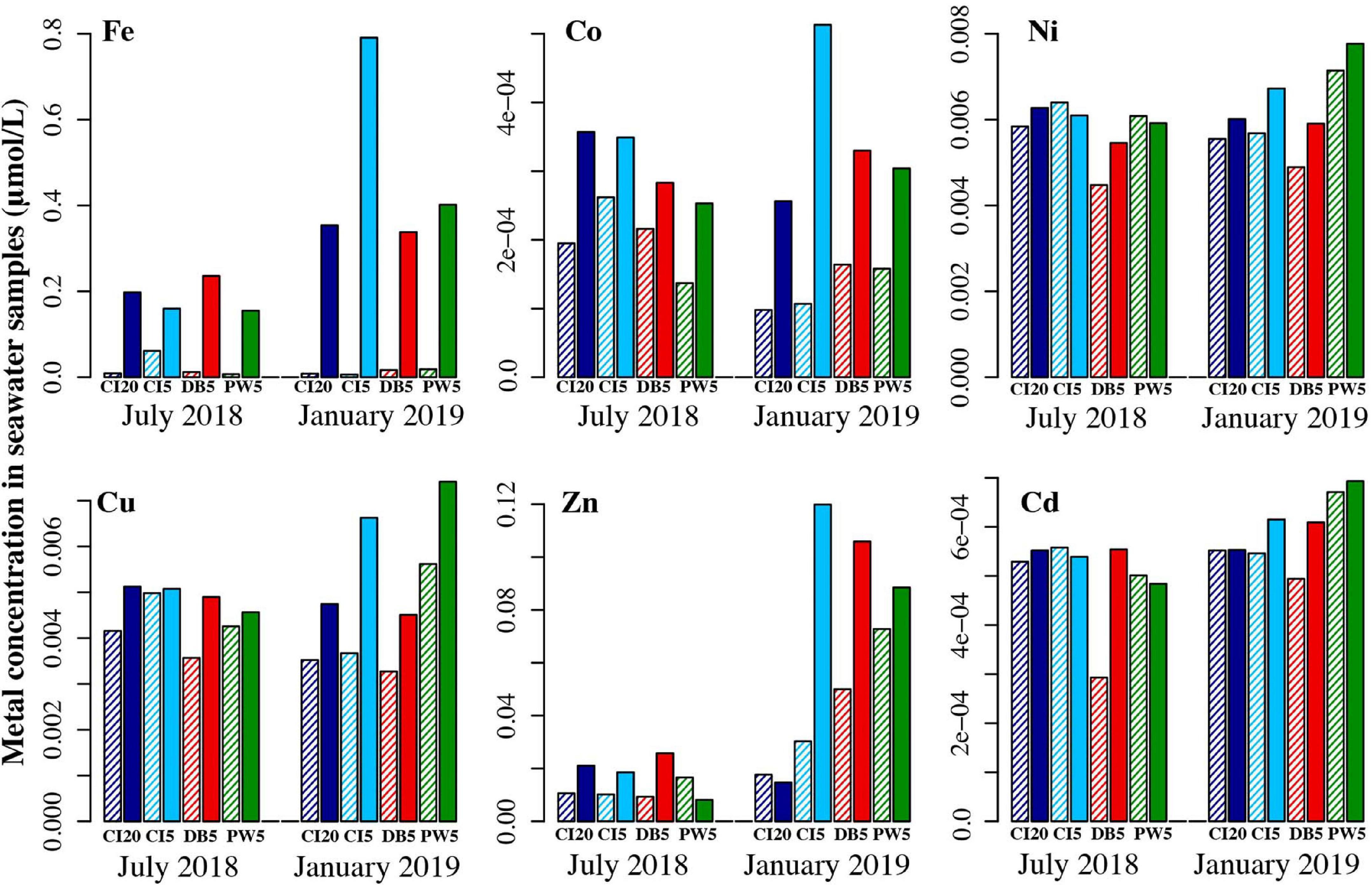
Figure 3. Trace metal analysis of seawater samples collected at the sites when the shellfish cages were deployed (July 2018), and 6 months after deployment began (January 2019). For each pair, the first bar (striped) is the filtered seawater sample, and the second bar (solid) is the unfiltered seawater sample—comparing the two should allow determination of what metals were dissolved in the seawater as opposed to in particulate matter. Dark blue = Carr Inlet 20 m, light blue = Carr Inlet 5 m, green = Point Wells 5 m, and red = Dabob Bay 5 m.
Trace Metal Tissue Analysis
For oysters, no relationships were found significant in the regressions comparing tissue metal concentrations to metals in filtered water (Figure 4). For unfiltered seawater samples, only Fe had a significant relationship between oyster tissue and seawater concentrations in July (R2 = 0.156, p = 0.0082). In January, the only significant relationship showed the concentration of Zn in oyster tissue actually decreased as concentrations of Zn in unfiltered seawater increased (R2 = 0.319, p < 0.0001 (Figure 5).
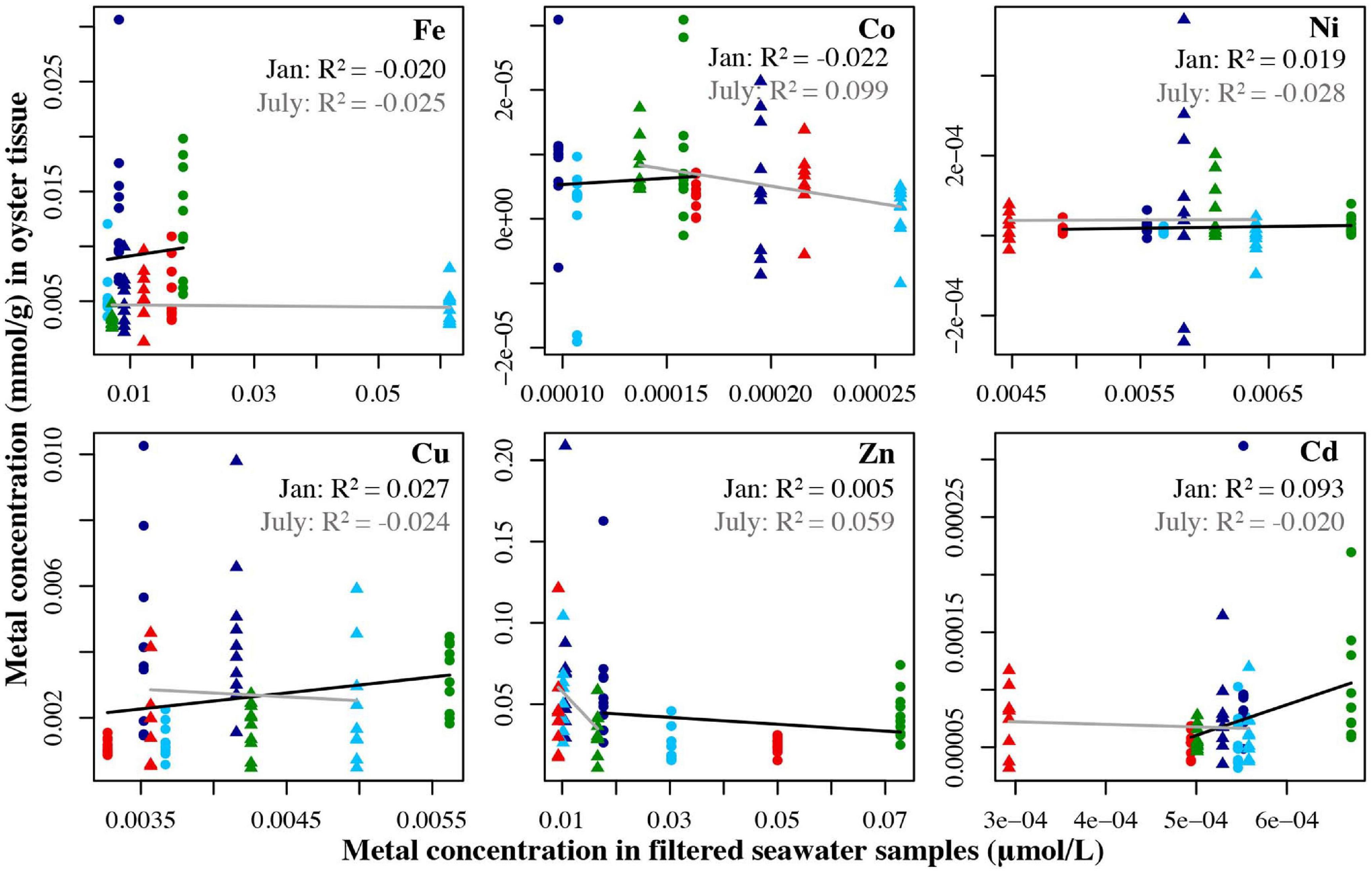
Figure 4. Metal concentration (μmol/L) in filtered seawater samples from July 2018 and Jan 2019 plotted against the metal concentration the oyster tissue samples (mmol/g) from the four locations collected in July 2019 and Jan 2019. Circles represent the January samples, triangles represent the July samples. Dark blue = Carr Inlet 20 m, light blue = Carr Inlet 5 m, green = Point Wells 5 m, and red = Dabob Bay 5 m. Linear regression was used to assess the relationship between the two variables for Jan (black line) and July (gray line) separately.
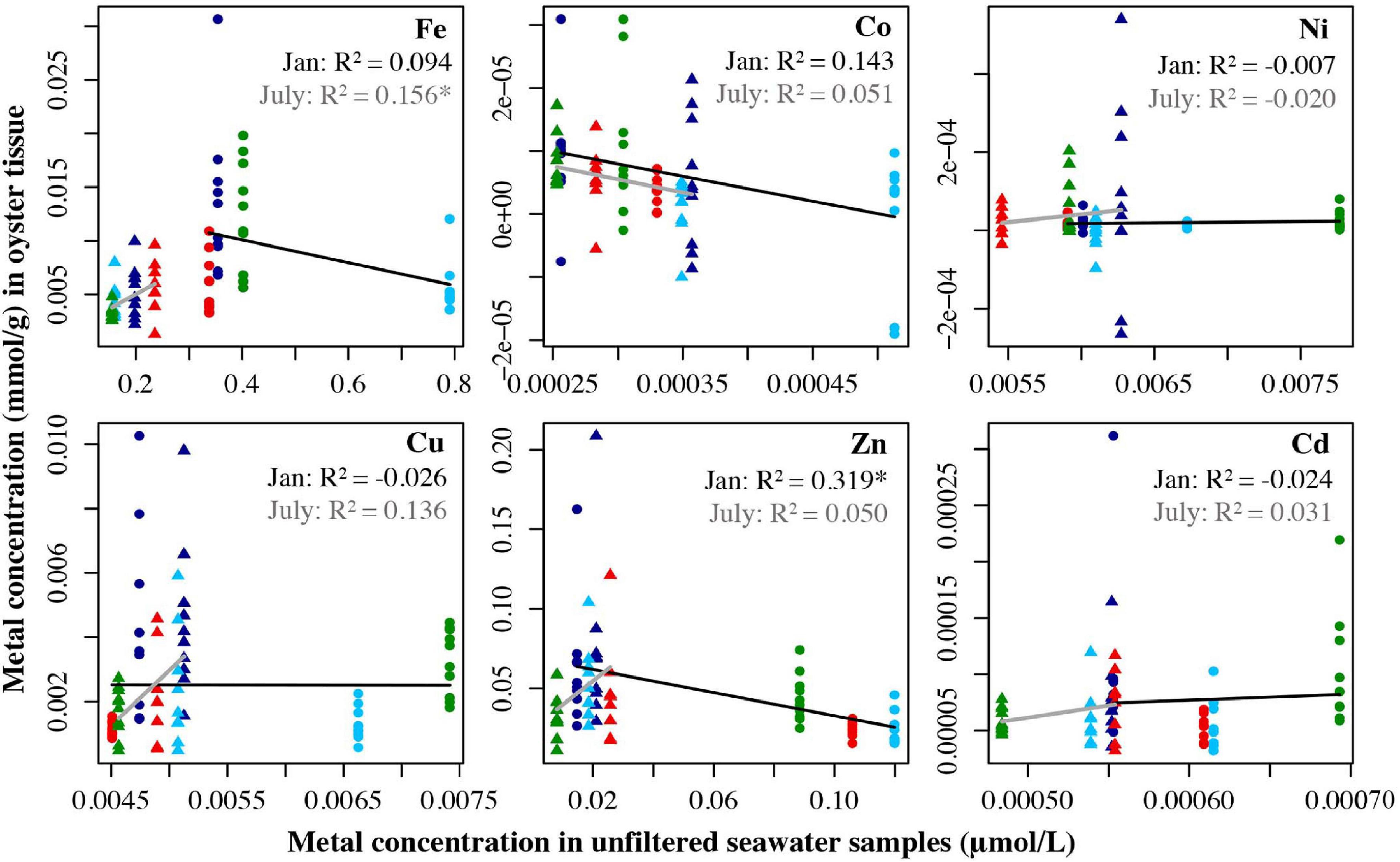
Figure 5. Metal concentration (μmol/L) in unfiltered seawater samples from July 2018 and Jan 2019 plotted against the metal concentration the oyster tissue samples (mmol/g) from the four locations collected in July 2019 and Jan 2019. Circles represent the January samples, triangles represent the July samples. Dark blue = Carr Inlet 20 m, light blue = Carr Inlet 5 m, green = Point Wells 5 m, and red = Dabob Bay 5 m. Linear regression was used to assess the relationship between the two variables for Jan (black line) and July (gray line) separately. Asterisk indicates the adjusted the R2 value is significant after Bonferroni correction (alpha of 0.0083).
For mussels, no metals had a significant relationship between tissue and filtered water for the January data. For the July filtered water data, two metals had significant relationships between the tissue and unfiltered water, Fe (R2 = 0.201, p = 0.003) and Co (R2 = 0.441, p < 0.0001) (Figure 6). For the unfiltered data in January, Fe (R2 = 0.251, p < 0.001), Co (R2 = 0.566, p < 0.0001), and Zn (R2 = 0.271, p = 0.0003) all showed significant negative relationships between tissue and seawater concentrations in January. For July, Cd (R2 = 0.226, p = 0.002) had a significant positive relationship between tissue concentration and seawater concentration (Figure 7). Trace metals in shellfish tissue represent bioaccumulation of trace metals over time, whereas water samples represent one discrete daily collection, thus caution should be taken when drawing conclusions from these comparisons.
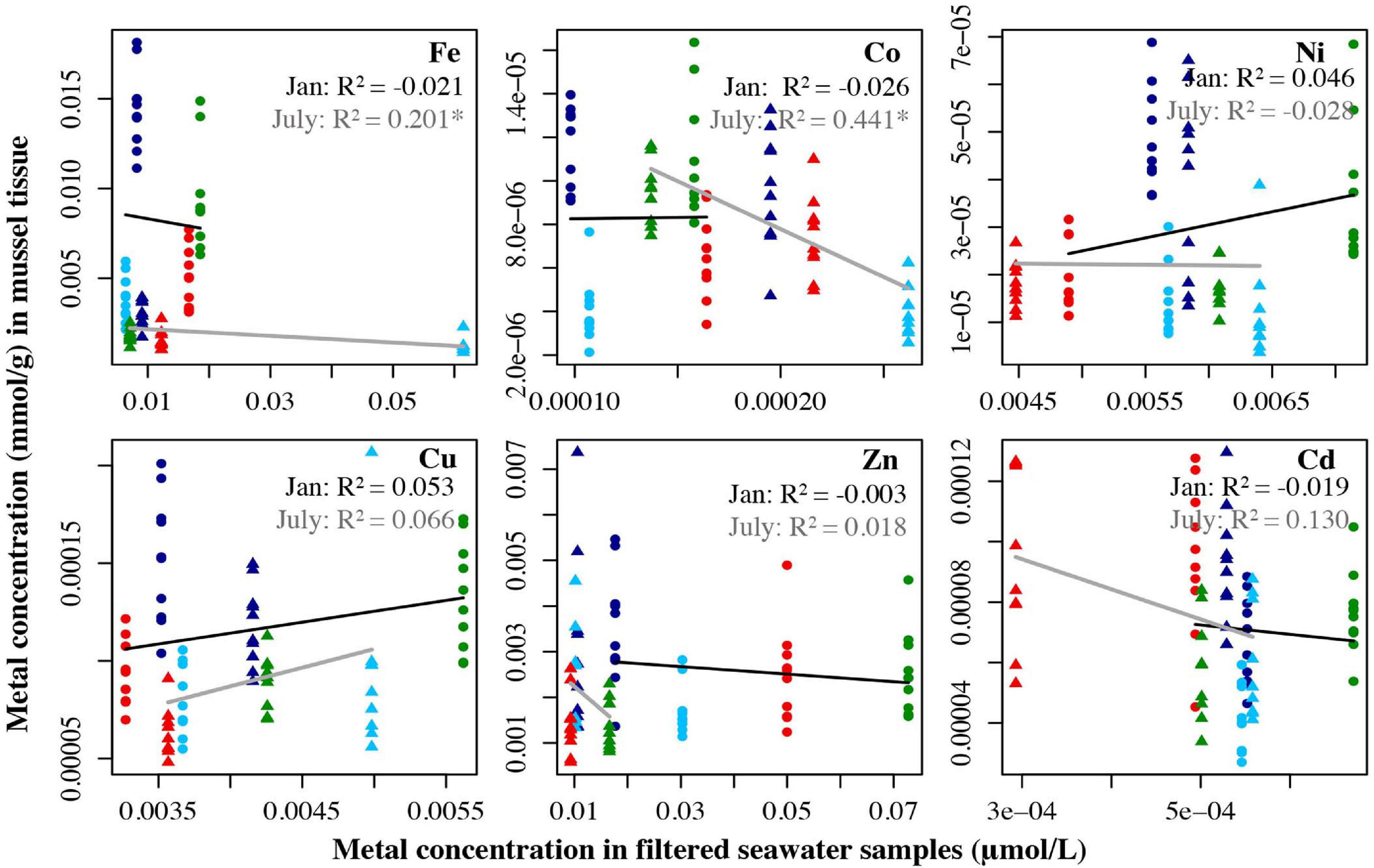
Figure 6. Metal concentration (μmol/L) in filtered seawater samples from July 2018 and Jan 2019 plotted against the metal concentration of mussel tissue samples (mmol/g) from the four locations collected in July 2019 and Jan 2019. Circles represent the January samples, triangles represent the July samples. Dark blue = Carr Inlet 20 m, light blue = Carr Inlet 5 m, green = Point Wells 5 m, and red = Dabob Bay 5 m. Linear regression was used to assess the relationship between the two variables for January (black line) and July (gray line) separately. Asterisk indicates the adjusted the R2 value is significant after Bonferroni correction (alpha of 0.0083).
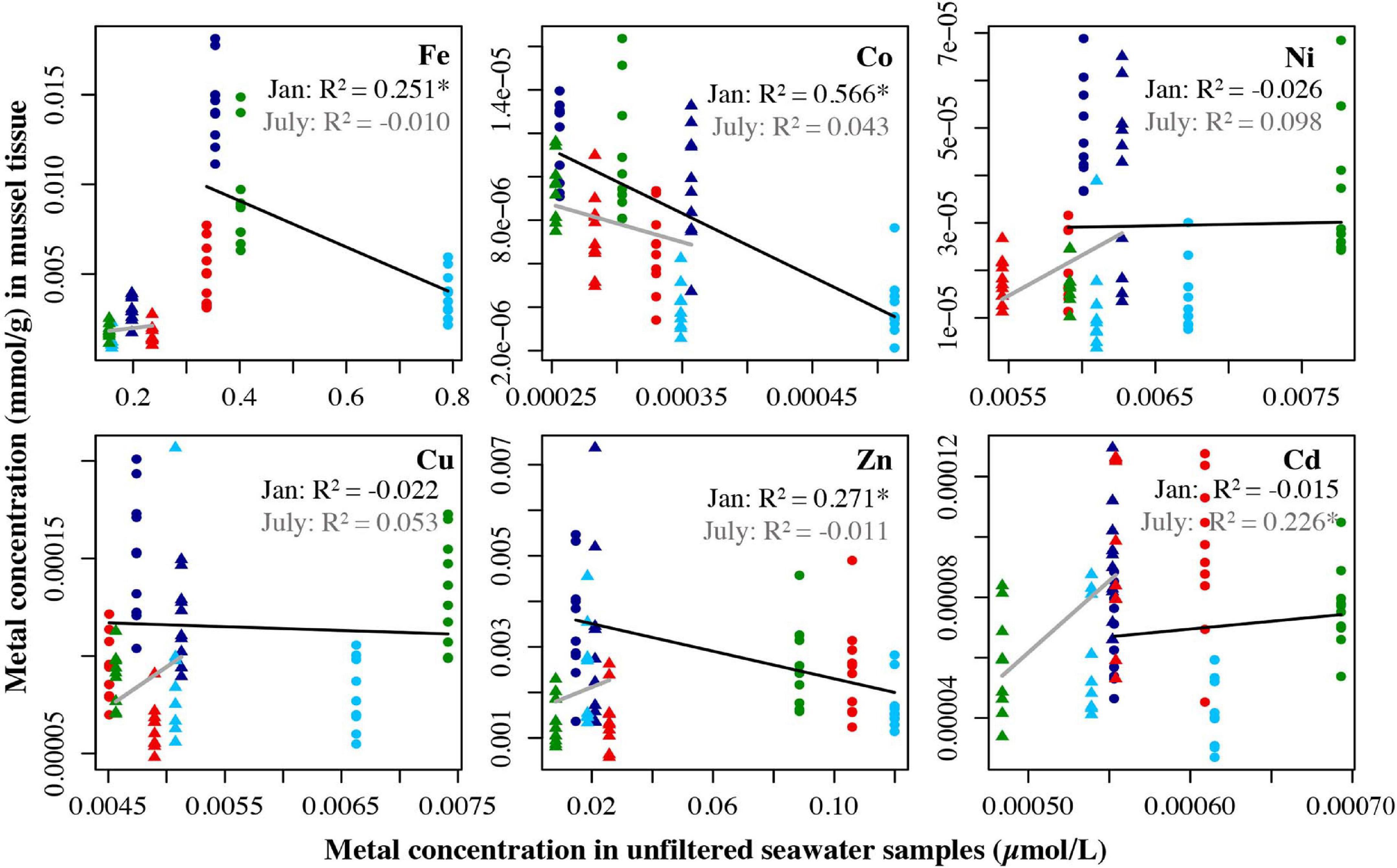
Figure 7. Metal concentration (μmol/L) in unfiltered seawater samples from July 2018 and Jan 2019 plotted against the metal concentration of mussel tissue samples (mmol/g) from the four locations collected in July 2019 and Jan 2019. Circles represent the January samples, triangles represent the July samples. Dark blue = Carr Inlet 20 m, light blue = Carr Inlet 5 m, green = Point Wells 5 m, and red = Dabob Bay 5 m. Linear regression was used to assess the relationship between the two variables for January (black line) and July (gray line) separately. Asterisk indicates the adjusted the R2 value is significant after Bonferroni correction (alpha of 0.0083).
There was a significant difference in metal concentrations found when comparing the two species across both sampling periods (perMANOVA, p = 0.0001 with 10,000 permutations). Comparing each individual metal between the two species, oysters had higher concentrations than mussels of Zn and Cu in both sampling periods (p < 0.0001 for all), and in July, oysters had a higher concentration of Fe than mussels (p < 0.0001), while mussels in July had a higher concentration of Mg than oysters (p = 0.003). Notably, the average concentration of Zn and Cu in oysters were 19.4 and 25.2 times higher in oysters than in mussels respectively (Supplementary Table 3).
Oysters had higher variation in metal accumulation between sites in January than in July. In January, Carr Inlet 20 m most frequently had the highest average levels of metals, with Point Wells 5 m frequently having the second highest levels of metals. In July, almost no significant differences in metal accumulation were found between sites. Oysters from Carr Inlet 20 m showed significant seasonal changes for the most metals, with higher levels found in January than July (Figure 8 and Supplementary Table 4).
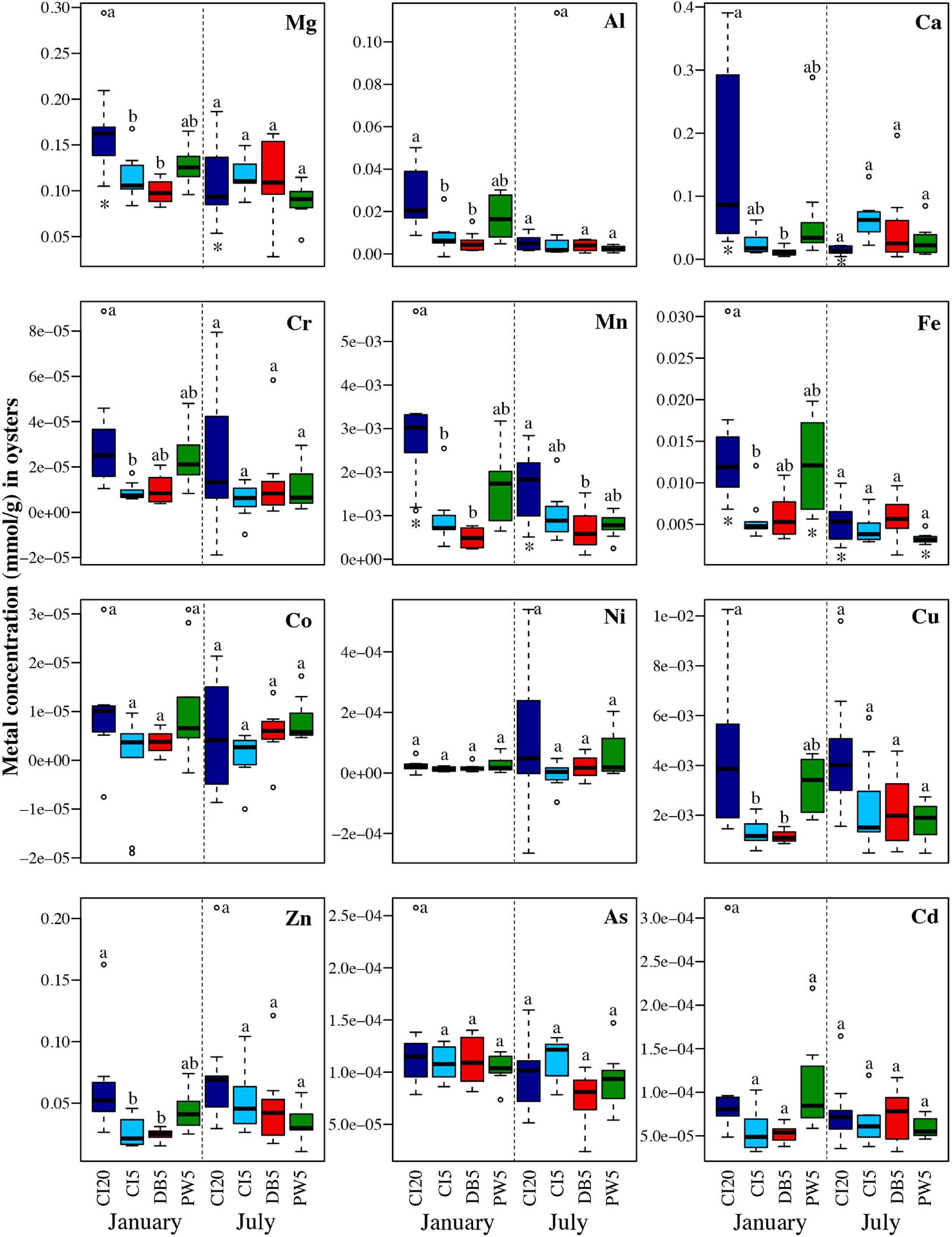
Figure 8. Concentrations in mmol/g for each of the twelve analyzed trace metals in oysters held for 6 months (January) and 1 year (July) in four locations: Carr Inlet 20 m (dark blue), Carr Inlet 5 m (light blue), Dabob Bay 5 m (red), and Point Wells 5 m (green). ANOVAs and Tukey Post-Hoc Tests with a Bonferroni correction were used to see if there were significant differences (alpha of 0.004) between location for January and July separately, and differences are indicated by letter above each boxplot. Separate ANOVA and Tukey Post-Hoc Tests were also completed to compare across time periods. Asterisks below the box plot indicate a significant difference (alpha of 0.004) in the concentration of a metal at one site between January and July.
In mussels, trace metal concentrations were generally higher in January than in July. Carr Inlet 20 m generally had the highest concentrations of metals, with Point Wells 5 m having the second highest concentrations. One notable exception was the highest average concentrations of Cd in both January and July at Dabob Bay 5 m. Mussel bioaccumulation of Al, Fe, and Cr had lower variability in July than in January (Figure 9 and Supplementary Table 4).
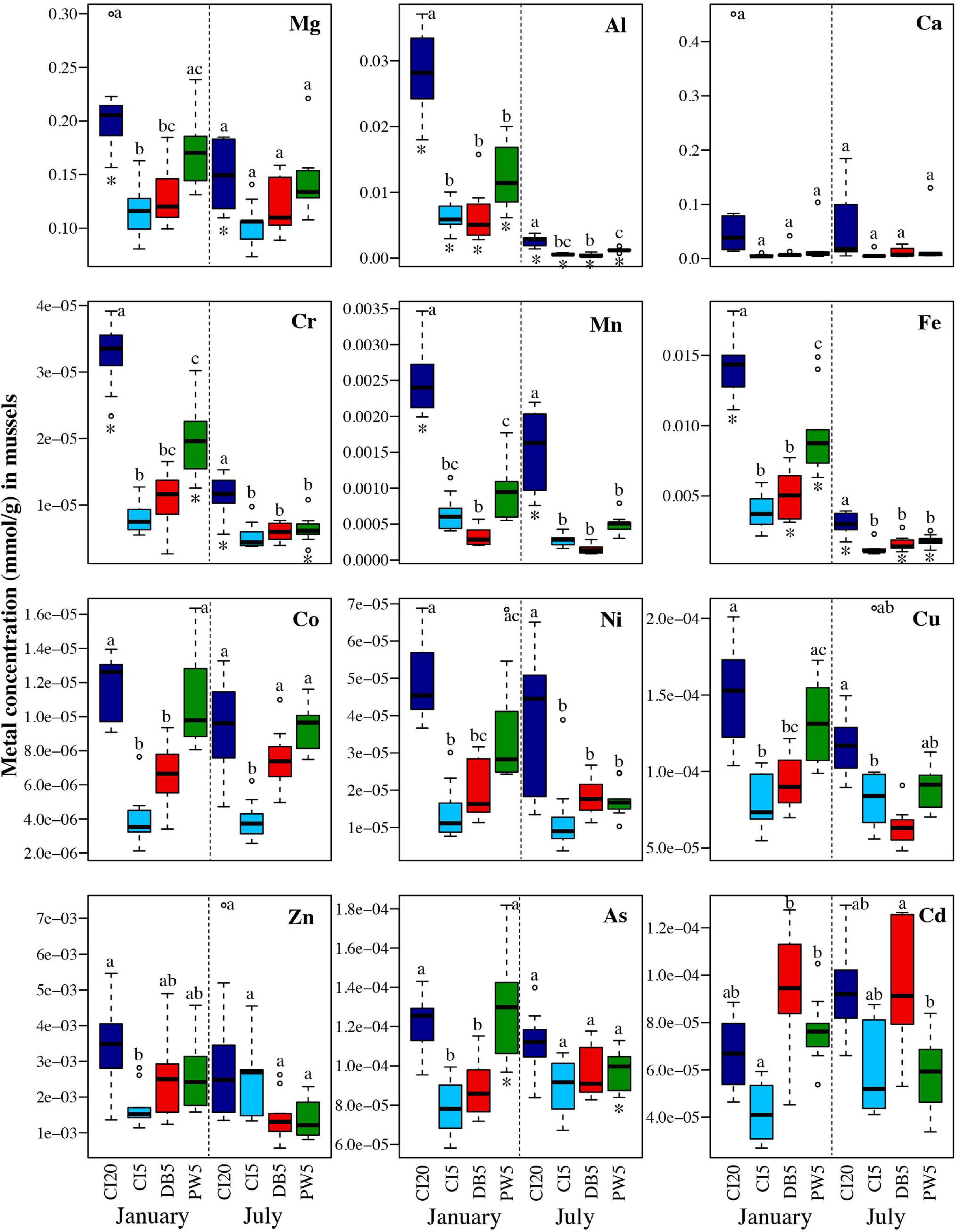
Figure 9. Concentrations in mmol/g for each of the twelve analyzed trace metals in mussels held for 6 months (January) and 1 year (July) in four locations: Carr Inlet 20 m (dark blue), Carr Inlet 5 m (light blue), Dabob Bay 5 m (red), and Point Wells 5 m (green). ANOVAs and Tukey Post-Hoc Tests with a Bonferroni correction were used to see if there were significant differences (alpha of 0.004) between location for January and July separately, and differences are indicated by letter above each boxplot. Separate ANOVA and Tukey Post-Hoc Tests were also completed to compare across time periods. Asterisks below the box plot indicate a significant difference (alpha of 0.004) in the concentration of a metal at one site between January and July.
Shellfish size varied between sites and sampling periods (Supplementary Table 5). Looking at both January and July data together, the sampled mussels were smaller at CI 20 m than at CI 5 m (p < 0.0001), DB 5 m (p < 0.0001), and PW 5 m (p = 0.0002). Mussels were also smaller at PW 5 m than at CI 5 m (p = 0.0024). Overall, mussels sampled were larger during the July sampling than during the January sampling (p = 0.0008).
For oysters, the difference in size between January and July sampling was not significant (p = 0.2048). The oysters from CI 20 m were smaller than those from CI 5 m (p = 0.0003) and DB 5 m (p = 0.0018), but no other relationships between sites were significant with regard to dry weight of oysters (Supplementary Table 5).
Smaller shellfish generally had higher concentrations of metals (Figures 10, 11). Metal concentration decreased significantly with increasing oyster mass for eight of the metals analyzed using an exponential regression: Mg (R2 = 0.14, p = 0.0004), Al (R2 = 0.14, p = 0.0004), Cr (R2 = 0.13, p = 0.0007), Mn (R2 = 0.37, p < 0.0001), Fe (R2 = 0.25, p < 0.0001), Cu (R2 = 0.44, p < 0.0001), Zn (R2 = 0.41, p < 0.0001), and Cd (R2 = 0.38, p < 0.0001) (Figure 10).
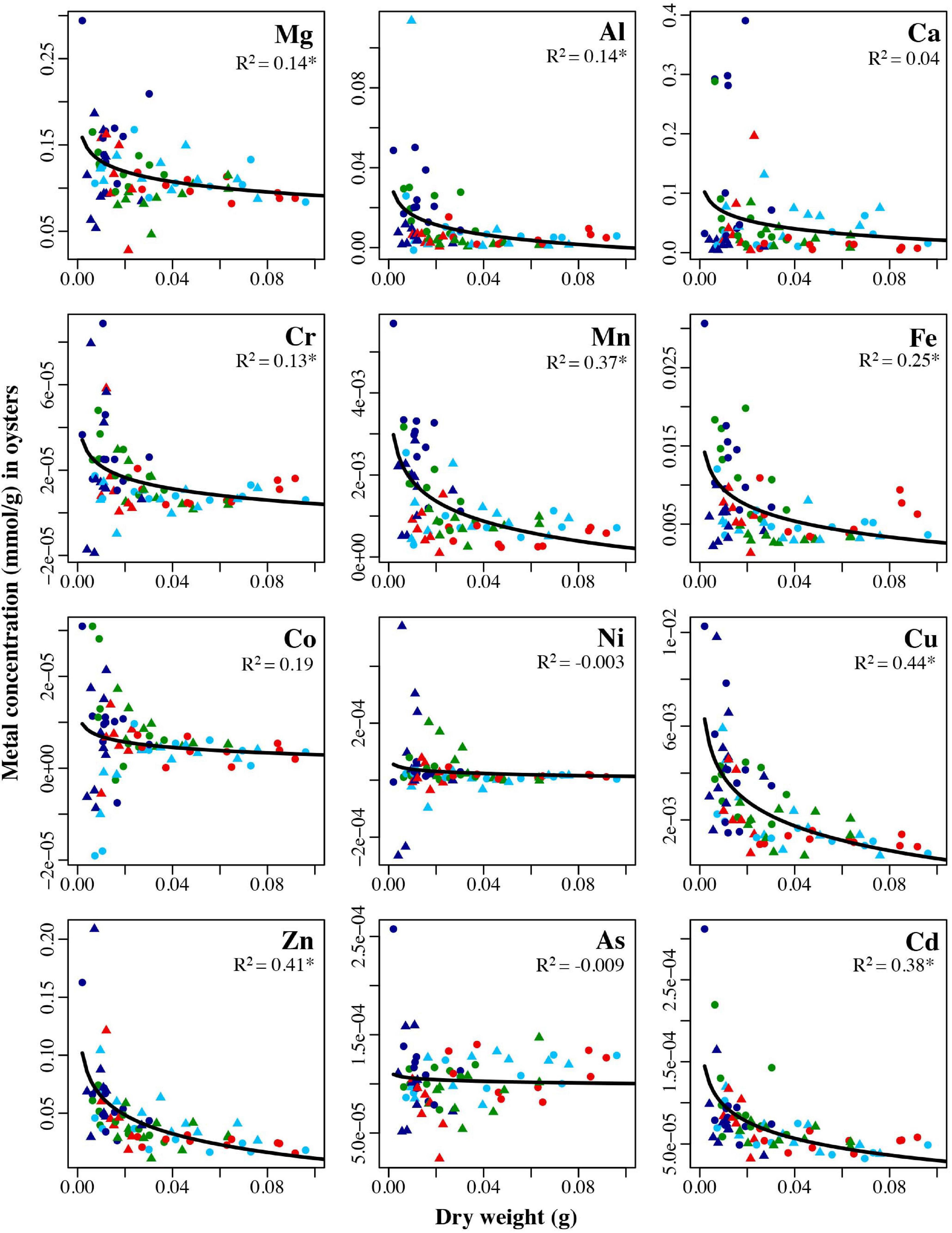
Figure 10. Concentrations in mmol/g for each of the twelve analyzed trace metals in oysters held for 6 months (January: circles) and 1 year (July: triangles) in four locations: Point Wells 5 m (green), Dabob Bay 5 m (red), Carr Inlet 5 m (light blue), and Carr Inlet 20 m (dark blue), all plotted against the dry weight (grams) of the oysters. Adjusted R2 values from exponential regression are shown in each panel. Asterisk indicates the R2 value is significant after Bonferroni correction (alpha of 0.004).
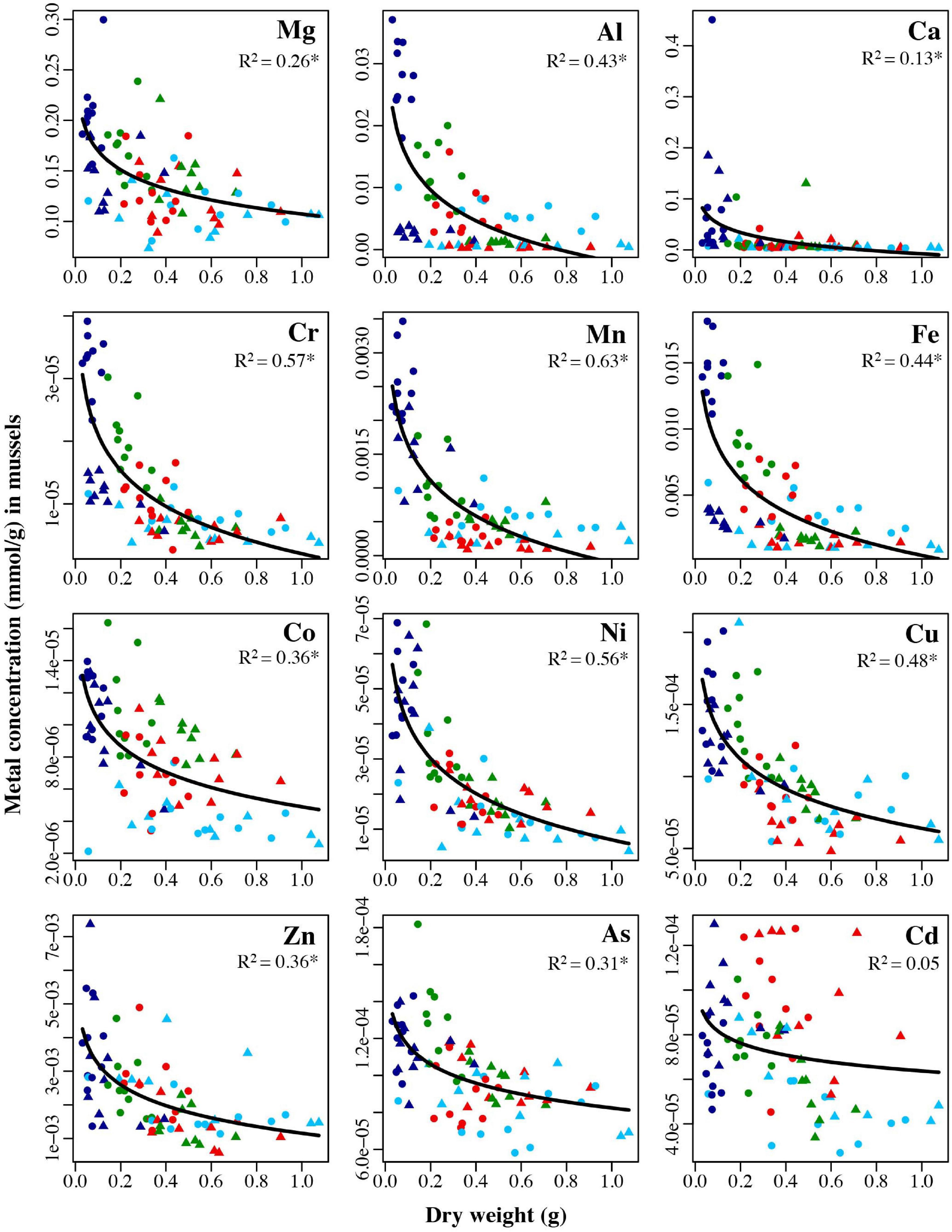
Figure 11. Concentrations in mmol/g for each of the twelve analyzed trace metals in mussels held for 6 months (January: circles) and 1 year (July: triangles) in four locations: Point Wells 5 m (green), Dabob Bay 5 m (red), Carr Inlet 5 m (light blue), and Carr Inlet 20 m (dark blue), all plotted against the dry weight (grams) of the oysters. Adjusted R2 values from exponential regression are shown in each panel. Asterisk indicates the R2 value is significant after Bonferroni correction (alpha of 0.004). One mussel sample that weighed ∼ 0.15 g was not graphed to better view the majority of samples, but was included in analyses.
For mussels, the negative relationship between mass and metal concentration was significant for every metal analyzed except Cd: Mg (R2 = 0.26, p < 0.0001), Al (R2 = 0.43, p < 0.0001), Ca (R2 = 0.13, p = 0.0006), Cr (R2 = 0.57, p < 0.0001), Mn (R2 = 0.63, p < 0.0001), Fe (R2 = 0.44, p < 0.0001), Co (R2 = 0.36, p < 0.0001), Ni (R2 = 0.56, p < 0.0001), Cu (R2 = 0.48, p < 0.0001), Zn (R2 = 0.36, p < 0.0001), As (R2 = 0.31, p < 0.0001) (Figure 11).
Principal component analysis for oysters revealed that principal components 1 and 2 explained 58.3% and 12.9% of the variance for January sampling, and explained 39.9 and 19% of the total variance for July sampling. The first principal component from the January sampling data, and the first two principal components from the July sampling data, explained a higher percent of the variance than would be expected using the Broken Stick model. The PCA showed that Carr Inlet 20 m site had the largest variability in metal concentration during both sampling times (January and July). Carr Inlet 5 m, in contrast, had considerably smaller variability in sample concentration at the two time points. The variability in metal concentrations relative to other sites increased between January and July for Dabob Bay 5 m but decreased for Point Wells 5 m. All metals were more closely correlated in January, while in July they diverged more into two groups, with Ni, Cr, and Co correlated with each other but not with the rest of the 12 metals (Figure 12).
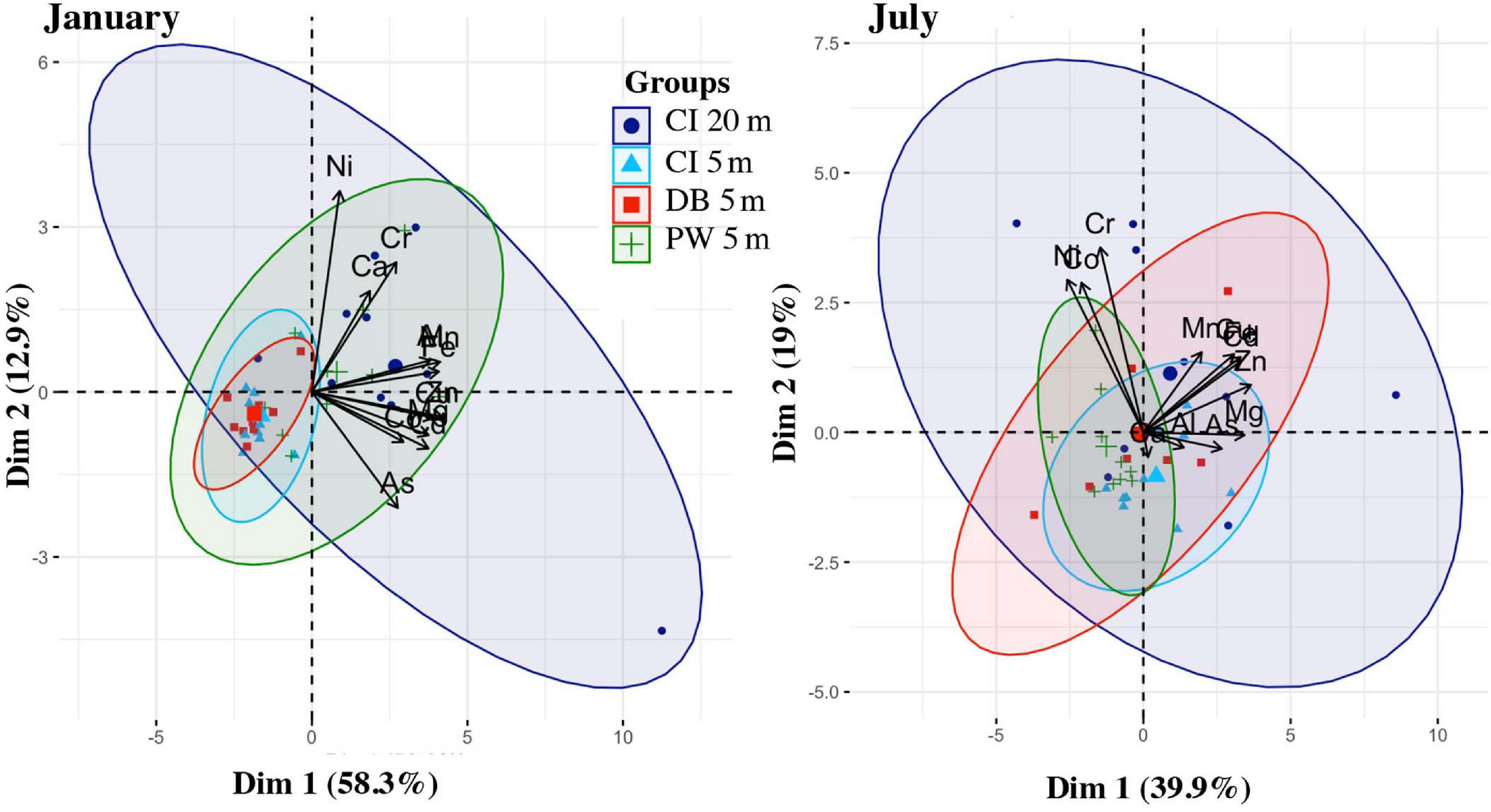
Figure 12. PCA of the trace metals data from oysters from January and July, colored by location (Carr Inlet 20 m = dark blue, Carr Inlet 5 m = light blue, Dabob Bay 5 m = red, Point Wells 5 m = green).
Principal component analysis for mussels revealed that principal components 1 and 2 explained 67.5 and 12% of the variance for January sampling, and explained 53.6 and 15.4% of the total variance for July sampling. Only the first principal component from both sampling periods explained a higher percent of the variance than would be expected using the Broken Stick model. The PCA showed that Carr Inlet 20 m was associated with overall higher metal concentrations during both the January and July sampling, and had larger variability in metal concentrations. The most evident change between seasons is with Cd, which is more correlated with the other metals in July than in January. Based on location in multivariate space, Dabob Bay 5 m and Point Wells 5 m were more influenced by higher Cd during the January sampling. Ca was not correlated with other metals in either time period (Figure 13).
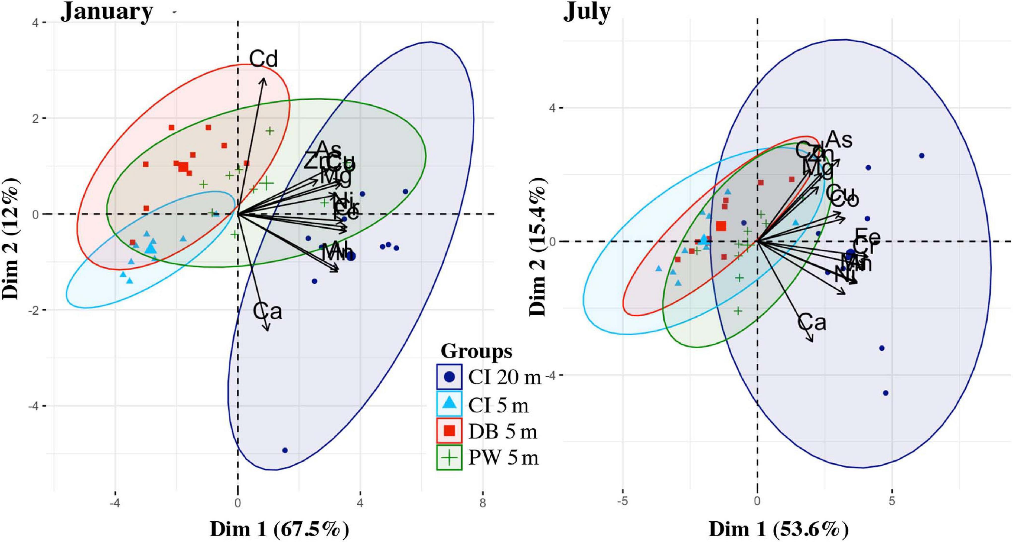
Figure 13. PCA of the trace metals data from mussels from January and July, colored by location (Carr Inlet 20 m = dark blue, Carr Inlet 5 m = light blue, Dabob Bay 5 m = red, Point Wells 5 m = green).
Average values of metals that would be consumed if a person ate 0.5 lb of Puget Sound mussels or oysters per day were sometimes above “average daily intake” or “adequate intake” levels (as defined for adults in the United States and Australia/New Zealand, respectively), but these metals (Cr, Mn, Al, Co, Ni) do not have regulated maximum values for consumption. This occurred most often in Carr Inlet 20 m samples (Table 2; Faroon et al., 2004; Agency for Toxic Substances and Disease Registry, 2005, 2008; Capra, 2006).
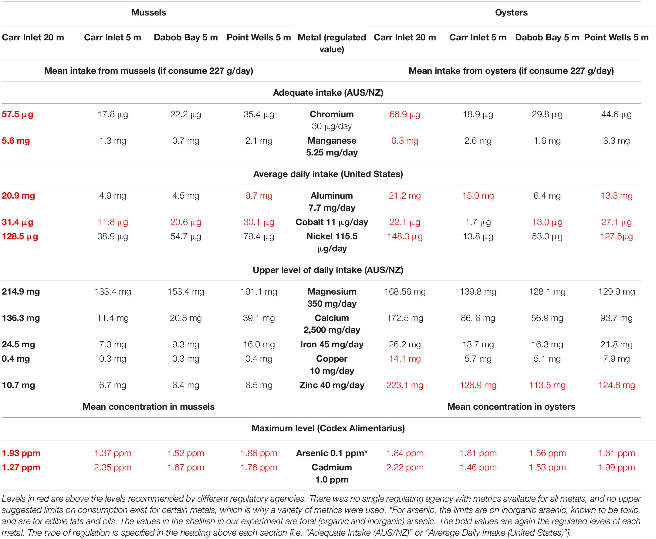
Table 2. Average concentrations of metals found in mussels and oysters from each of the four sites compared to the average or maximum recommended levels available for each metal.
For those metals where there are upper recommended daily intake levels (Mg, Ca, Fe, Cu, and Zn), only copper (at Carr Inlet 20 m) and zinc (at all sites) were over the recommended level for oysters, and no metals were over the recommended level for mussels (upper recommended daily intake in Australia/New Zealand defined as the “highest average daily nutrient intake level likely to pose no adverse health effects”) (Capra, 2006). Codes Alimentarius, the international commission that sets food guidelines, only provides maximum allowable limits for inorganic arsenic, but the levels we measured were organic and inorganic arsenic together, so a direct comparison cannot be made (Codex Alimentarius Commission, 2015). Cadmium also has a maximum level permitted in mollusks by Codex Alimentarius, and in some cases the estimates from Puget Sound shellfish were over these levels (Table 2; Codex Alimentarius Commission, 2015).
Discussion
This study used experimental data from the field to investigate how effects of temperature, pH, and DO are associated with the accumulation of trace metals in mussels and oysters from Puget Sound.
Spatial and Seasonal Variability in Shellfish Trace Metal Bioaccumulation
Our results provide evidence that (1) lower pH is associated with higher metal concentrations in shellfish, and (2) depth may have more impact than site on metal bioaccumulation in Puget Sound. The deepest location, Carr Inlet 20 m, showed the lowest pH and the highest bioaccumulation in both oysters and mussels. Low pH has been shown to increase the solubility of certain trace metals. For example, models indicate a pH shift from 8.1 to 7.4 could increase the water solubility of Fe(III) by 40%, which would make it more bioavailable to plankton (Brand, 1991; Millero et al., 2009), and in turn likely available to higher trophic levels. It is important to note that other variables may play a role in the shellfish physiological performance and bioaccumulation of trace metals. Carr Inlet 20 m also had lower light levels and lower and less variable dissolved oxygen levels, which may impact shellfish directly as well as indirectly through plankton abundance (Alma, n.d.in prep, Unpublished).
Carr Inlet 20 m showed the largest seasonal differences in bioaccumulation. At this site we found seasonal changes in metal abundance in mussels and oysters (Mg, Al, Cr, Mn, and Fe for mussels, Mg, Ca, Mn, and Fe for oysters), with the higher levels for each of these metals occurring in January. This site had experienced its lowest pH levels in the months leading up to this sampling, potentially causing the higher metal bioaccumulation. However, we did not see this trend at shallow sites which also had lower pH leading up to the January sampling, suggesting that there are other physical and biological factors that also fluctuate seasonally that may impact the abundance of trace metals in our study.
In our study, the highest concentrations of cadmium in mussels were found at Dabob Bay (which on average had the highest pH but showed extreme drops in pH levels during winter), and at Carr Inlet 20 m in the July sampling (the site which overall had the lowest pH). The variability in results of previous laboratory studies (Millero et al., 2009; Lacoue-Labarthe et al., 2012; Ivanina et al., 2013; Belivermiş et al., 2016; Shi et al., 2016; Nardi et al., 2018) and our field study may be an indication that some unknown environmental factor—separate from aqueous speciation—is influencing the accumulation of cadmium in all these studies. In the field, Carr Inlet 20 m and Point Wells 5 m also had higher copper concentrations for mussels, and Carr Inlet 20 m had higher copper concentrations for oysters. These two sites are colder, have less variability in dissolved oxygen, and have slightly lower pH, and this lower pH is consistent with increased copper uptake seen in other studies on shellfish (Ivanina et al., 2013; Götze et al., 2014; Hawkins and Sokolova, 2017; Cao et al., 2018, 2019).
Multivariate analyses also revealed that most of the metals were positively correlated to each other—i.e., some samples have higher amounts of all the metals or few of all the metals, as opposed to some sites having more of one and less of another metal. Our evidence did not link warmer sites (which would have caused increased metabolism) to higher levels of metals in shellfish.
Trace Metals in the Environment
For both mussels and oysters, there were few significant positive correlations between the concentrations of trace metals in seawater and tissue samples (and some were even negative). This does not establish a clear relationship between water and tissue concentrations for either species or for any specific metal and does not explain the differences in metal accumulation in shellfish between sites. Previous studies did not find correlation between metal concentrations in filtered water and mussel tissue (Fowler and Oregioni, 1976). This may have been due to the ability of filter feeders to ingest metals that are suspended in particulate matter in the water, as particulate matter is not accounted for in filtered water samples (Fowler and Oregioni, 1976). We had expected to explain this discrepancy further by analyzing both filtered and unfiltered water samples, but also found little correlation between metal concentration in shellfish and seawater, indicating that including particulate matter in the analysis still did not account for how the shellfish are ingesting and processing trace metals. The field seawater samples did reveal generally higher concentrations in unfiltered samples, supporting the idea that more metals are available if shellfish ingest both the dissolved and particulate matter in the water. The ability of shellfish to selectively feed—whether this results in a higher or lower intake of metals than through random feeding, could be responsible for the discrepancy (Purroy et al., 2018). This lack of correlation could also be confounded by the difference in sizes between shellfish at different sites. It is important to note that water samples for trace metals were collected during specific dates, whereas trace metals in shellfish provide a time-integrated image of metals. Lack of more pronounced correlations could be due to this difference in the nature of sampling from the two sources.
Sediment likely did not play a large role in the metal concentrations in these specific shellfish because the shellfish cages were suspended on lines far above the substrate, as opposed to sitting directly on the substrate. Aquaculture techniques including float bags and mussel rafts similarly grow shellfish suspended above the substrate. We do note, however, than many wild shellfish and shellfish used for aquaculture in Puget Sound do reside directly on the sediment.
Chemical analysis of sediment in Puget Sound was conducted between 1989 and 2015 in areas with close proximity to our research sites (Partridge et al., 2018). Results of this study show that overall, chromium, copper, and zinc levels were higher in the central Puget Sound sites than the South Puget Sound sites, and lower at the Hood Canal site (Partridge et al., 2018). The Sediment Chemistry Index values (which compare ratios of concentration to Sediment Quality Standards for 39 chemicals, a subset of which are metals) for the Hood Canal site, central Puget Sound sites, and one of the south Puget Sound sites are all very similar. The other south Puget Sound site, which is close to the industrial port of Tacoma, has considerably more variable and on average worse chemical index values, indicating higher exposure to chemicals at this site (Long et al., 2013; Partridge et al., 2018). Results from our study overall showed higher metal concentrations in shellfish at the 20 m south Puget Sound site (Carr Inlet), and in some cases high concentrations in shellfish at the central Puget Sound site (Point Wells). While the shellfish separation from the substrate makes it unlikely, our results may be a reflection of different sediment metal concentrations impacting the shellfish. It seems more likely that our results are unrelated to sediment concentrations, or the concentration of metals in shellfish and sediment may be affected by similar processes.
Shellfish Size and Trace Metal Accumulation
We found that trace metal bioaccumulation was higher in shellfish of smaller size. Higher metal concentration in smaller shellfish could be due to a residual effect of a prior metal signal from the common pool the shellfish were sourced from. The shellfish that grew less after being deployed in the cages would have less tissue to “dilute” that original signal. Because we sampled tissue as opposed to shell, we would expect some turnover in metal concentration with time, so this seems unlikely, but is a possibility. This trend could also be due to localization of metals to specific regions of the shellfish body if the relative contribution of these regions to total dry weight changes with age and size. For example, if metals accumulated more in internal organs as opposed to the lipids of the shellfish, then they could appear more concentrated in smaller shellfish when these organs make up more of the dry weight. Various other studies have focused on specific tissues within the shellfish such as the digestive gland of oysters or mantle cells of clams (Ivanina et al., 2013), and it has been noted that some metals tend to accumulate more in certain oyster tissues (Wang et al., 2018). Our study used the entire shellfish tissue to obtain a measurement of bioaccumulation per individual because the entire soft tissue of mussels and oysters is typically consumed by humans. The inverse relationship between metal concentration and size could influence the values we obtained at Carr Inlet 20 m. The shellfish at that location showed higher metal concentrations and weighed less than shellfish from other sites.
Other studies have also noted, both incidentally and intentionally, relationships between shellfish size and metal accumulation. In Mytilus species, it was noted that cadmium concentrations were independent of size, while zinc, manganese, nickel, and iron all had higher concentrations in smaller mussels (Boyden, 1977). For oysters (Ostrea spp.), previous studies found that cadmium and zinc concentrations were independent of body size, but zinc concentrations were more variable in polluted environments. For copper, it was noted that particularly large individuals took longer to equilibrate to the local copper conditions (Boyden, 1977)—corresponding to the slower (relative to mussels) depuration rates of copper in oysters noted in other studies (Han et al., 1993). Further, size may interact with oceanographic variables such as pH to influence accumulation: juvenile mussels (M. galloprovincialis) were found to have increasing cadmium concentration in lower pH treatments, but the same effect was not found for adults (Sezer et al., 2020). These size differences in part can be explained by higher metabolic rate and higher surface area to volume ratio of smaller juveniles compared to adults (Sezer et al., 2020).
In addition to size, the reproductive stage and sexual maturation of bivalves may also impact the concentration of trace metals in the tissue (Fattorini et al., 2008). In a complementary study to ours, gonad histology data was collected for oysters and mussels (different individuals than those used for trace metal analysis) located at our field sites (Alma, n.d.). Overall findings indicate that there were no differences in gonad development between oysters from different sites or between the two time periods (Alma, n.d.). However, mussels were in later maturation stages (some having more developed gonads and some having already spawned out) in July than in January. Mussels from Carr Inlet 20 m, which were smaller and showed the highest levels of trace metals, had mostly spawned by both collection times. Mussels from Dabob Bay had mostly spawned by the July collection, while there were still some that had not yet spawned from Point Wells 5 m and Carr Inlet 5 m by July (Alma, n.d.). Multiple studies have noted that the higher fraction of weight in gonadal tissue that occurs seasonally can dilute trace metals in the shellfish tissue (Soto et al., 2000; Fattorini et al., 2008). As the mussels from Carr Inlet 20 m had already spawned, gonadal tissue was not a large fraction of their weight and this may explain some of the higher concentration of metals at that site. Overall, in our study trace metal levels were generally found to be higher in mussels from the January sampling when gonads were less developed and fewer mussels had spawned. It is likely in our study that size and maturity of shellfish both had impacts on the concentration of trace metals.
Trace Metal Accumulation in Oysters vs. Mussels
In addition to differences based on shellfish size and site, our study found clear differences in the metal accumulation between the two species. The oysters in our study had significantly higher levels of copper and zinc (about 25.2 and 19.4 times higher, respectively), which may in part be due to a faster turnover of copper in the mussel species (Han et al., 1993). A previous study focusing on the depuration of copper and zinc by bivalves in Taiwan transplanted from polluted to clean waters showed faster depuration rates of copper in blue mussels than green oysters (Han et al., 1993). In the Patuxent River Estuary in Maryland, another study found that eastern oysters accumulated varying amounts of copper depending on site, while mussels had more constant levels of copper throughout the estuary (Riedel et al., 1995). In our study, mussels and oysters experienced the same environments with common food sources, indicating that their species-specific responses to the environment contributed to their different bioaccumulation rates (Riedel et al., 1995). Previous studies have also shown evidence that mussels have some capacity to metabolically regulate trace metal concentrations of zinc and copper (Scott and Major, 1972; Davenport and Manley, 1978; Phillips and Yim, 1981), a trait that oysters do not possess, resulting in the higher accumulation in oysters (Phillips and Yim, 1981). They also note that oysters and mussels have different pathways of trace-element incorporation. With iron, for example, oysters incorporate the metal into their shells while mussels incorporate more iron into the byssus (Phillips and Yim, 1981).
Multivariate trends we found between sites (most prominently the higher concentration of metals at Carr Inlet 20 m) stayed relatively consistent for mussels between the January and July samplings, but for oysters, PCA reveals a different pattern in prevalence of metals at certain sites between the two sampling times. This may be related to different abilities to regulate trace metal concentrations or different depuration times (Scott and Major, 1972; Davenport and Manley, 1978; Phillips and Yim, 1981; Han et al., 1993; Riedel et al., 1995). Alternatively, these patterns could reflect biological differences between the species—as faster filterers, oysters may change their internal concentrations of certain elements more rapidly than mussels (Wang et al., 2018). These physiological differences between species are important and emphasize the need for species-specific studies to better understand the mechanisms involved in accumulation and regulation of trace metals and how these species can or should be used as pollution indicators (Phillips and Yim, 1981). In addition, this could provide a physiological explanation for some of the discrepancies between seawater and tissue concentrations of trace metals we found in this study.
Applications to Aquaculture
The apparent trend of lower metal concentrations for larger shellfish is encouraging for the aquaculture industry, in that those mussels and oysters that are harvested and sold are generally of a larger size, and therefore would have lower concentration of metals by weight. Among the cages deployed at 5 m depths, the shellfish at Point Wells (Central Sound) had the highest concentrations of metals. This area of the central sound has less shellfish farming than the Dabob Bay site (Hood Canal), and the Carr Inlet site at 5 m (South Sound). The higher metal concentrations found in shellfish located at the Carr Inlet 20 m site reveal a notable effect of depth, which is important information for shellfish farmers—although most shellfish are grown in the intertidal, some mussels in Puget Sound are grown hanging from lines on rafts and reach deeper levels. Metal accumulation may be more of a concern for those shellfish, but again, our findings may have been influenced by the smaller size (slower growth) of shellfish at that depth.
While this was not a toxicology study, and the intention was to compare shellfish metal concentrations between sites and species as opposed to comparing them to regulatory levels, we did estimate concentrations of metals in the wet shellfish tissue to see whether they were comparable to regulations for daily intake, and in certain cases, maximum allowable levels. The most notable of our findings are the much higher concentrations of copper and zinc in oysters, which were in some cases over recommended daily values if an adult were to eat 0.5 pounds of shellfish daily. Shellfish are known to have particularly high concentrations of copper: The National Institute of Health found that three ounces of cooked eastern oyster could result in over 500% of the listed adult Daily Value for copper (National Institute of Health, 2020). Codex Alimentarius, the international commission that sets food guidelines, does not consider all metals to be contaminants. Copper, for example, is considered to have significance in terms of food quality, but not public health significance, so strict upper limits are not set (Codex Alimentarius Commission, 2015). Cadmium, however, is considered a contaminant by Codex, and cadmium pollution in Puget Sound shellfish has been studied, as levels over the Codex standard could be detrimental to the shellfish industry (Pacific Shellfish Institute, 2008). The commission set the limit as 1 ppm in molluscan shellfish in 2003, but later changed the limited to 2 ppm (Pacific Shellfish Institute, 2008). A study focused on Hood Canal oysters found that most shellfish were below this 2 ppm limit, but 15% exceeded it (Pacific Shellfish Institute, 2008). Our study had average levels over this 2 ppm limit at the Carr Inlet 5 m site for mussels and the Carr Inlet 20 m site for oysters—indicating higher levels in central sound than in Hood Canal.
The variation in metal concentrations between our sites indicates that water properties may have some impact on metal concentrations. The variability in trace metal accumulation we found in the field based on size, site, water properties, and depth all point to the necessity to continue testing trace metal accumulation at local levels, especially in regions with important aquaculture industries.
Data Availability Statement
The raw data supporting the conclusions of this article will be made available by the authors upon request, without undue reservation.
Author Contributions
EB completed the laboratory work, the statistical analyses, and wrote the manuscript. LA developed the experiment, conducted the fieldwork, completed the shellfish dissections, compiled the environmental data, and wrote the manuscript. TU ran the instrumentation, analyzed the data, and wrote the manuscript. AG, MM, and PM provided guidance and support during the field experiments and wrote the manuscript. JP-G planned the project, acquired the funding, supported the analysis, and wrote the manuscript. All authors contributed to the article and approved the submitted version.
Funding
This work was supported by the University of Washington startup funds, a NOAA Saltonstall-Kennedy Grant (NA17NMF4270222), and UW Royalty Research Fund (FA137468/A118587) grant awarded to JP-G, as well as a sub-award to JP-G from an MJ Murdock Charitable Trust grant (“Inductively Coupled Plasma-Mass Spectrometer”). Funders supported graduate students, field work, materials and supplies, chemical analyses, and publication charges.
Conflict of Interest
The authors declare that the research was conducted in the absence of any commercial or financial relationships that could be construed as a potential conflict of interest.
Acknowledgments
We would like to thank Miranda Roethler for her help with mapping, the other members of the Padilla-Gamiño lab at UW SAFS (Jeremy Axworthy, Corinne Klohmann, and Tanya Brown) for their support throughout analysis and writing, and Catherine A. Craighill for her assistance with figure editing and formatting. We would also like to thank Chris Archer, Robert Daniels, and Will Love for their assistance with SCUBA fieldwork; Jan Newton, John Mickett, and Ryan Newell for contributing to project planning, field deployments, and providing data from APL; the Northwest Environmental Moorings group for providing a diagram for one of our figures; and Parker MacCready for providing data from the LiveOcean Model. We would also like to thank Gordon King for providing mussels from Taylor Shellfish and Ryan Crim, Stuart Ryan, and Betsy Peabody for providing oysters from Puget Sound Restoration Fund.
Supplementary Material
The Supplementary Material for this article can be found online at: https://www.frontiersin.org/articles/10.3389/fmars.2021.636170/full#supplementary-material
References
Agency for Toxic Substances and Disease Registry (2005). Toxicological Profile for NICKEL. Washington, DC: US Department of Health and Human Services.
Agency for Toxic Substances and Disease Registry (2008). Toxicological Profile for Aluminum. Washington, DC: US Department of Health and Human Services.
Ashoka, S., Peake, B. M., Bremner, G., Hageman, K. J., and Reid, M. R. (2009). Comparison of digestion methods for ICP-MS determination of trace elements in fish tissues. Anal. Chim. Acta 653, 191–199. doi: 10.1016/j.aca.2009.09.025
Belivermiş, M., Warnau, M., Metian, M., Oberhänsli, F., Teyssié, J.-L., and Lacoue-Labarthe, T. (2016). Limited effects of increased CO2 and temperature on metal and radionuclide bioaccumulation in a sessile invertebrate, the oyster Crassostrea gigas. ICES J. Mar. Sci. 73, 753–763. doi: 10.1093/icesjms/fsv236
Boyden, C. R. (1977). Effect of size upon metal content of shellfish. J. Mar. Biol. Assoc. UK 57, 675–714. doi: 10.1017/s002531540002511x
Brand, L. E. (1991). Minimum iron requirements of marine phytoplankton and the implications for the biogeochemical control of new production. Limnol. Oceanogr. 36, 1756–1771. doi: 10.4319/lo.1991.36.8.1756
Brandenberger, J. M., Crecelius, E. A., and Louchouarn, P. (2008). Historical Inputs and Natural Recovery Rates for Heavy Metals and Organic Biomarkers in Puget Sound during the 20th Century. Washington, DC: ACS Publications.
Byrne, R., Kump, L. R., and Cantrell, K. J. (1988). The influence of temperature and pH on trace metal speciation in seawater. Mar. Chem. 25, 163–181. doi: 10.1016/0304-4203(88)90062-x
Cao, R., Liu, Y., Wang, Q., Dong, Z., Yang, D., Liu, H., et al. (2018). Seawater acidification aggravated cadmium toxicity in the oyster Crassostrea gigas: metal bioaccumulation, subcellular distribution and multiple physiological responses. Sci. Total Environ. 642, 809–823. doi: 10.1016/j.scitotenv.2018.06.126
Cao, R., Zhang, T., Li, X., Zhao, Y., Wang, Q., Yang, D., et al. (2019). Seawater acidification increases copper toxicity: a multi-biomarker approach with a key marine invertebrate, the Pacific Oyster Crassostrea gigas. Aquat. Toxicol. 210, 167–178. doi: 10.1016/j.aquatox.2019.03.002
Capra, S. (2006). Nutrient Reference Values for Australia and New Zealand: Including Recommended Dietary Intakes. Camperdown, NSW: National Health and Medical Research Council.
Chan, C. Y., and Wang, W.-X. (2018). A lipidomic approach to understand copper resilience in oyster Crassostrea hongkongensis. Aquat. Toxicol. 204, 160–170.
Codex Alimentarius Commission (2015). General Standard for Contaminants and Toxins in Food and Feed (Codex Stan 193-1995). Rome: Codex Alimentarius Commission.
Davenport, J., and Manley, A. (1978). The detection of heightened sea-water copper concentrations by the mussel Mytilus edulis. J. Mar. Biol. Assoc. UK 58, 843–850. doi: 10.1017/s0025315400056800
Environmental Protection Agency (1996). EPA Method 3050B Acid Digestion of Sediments, Sludges, and Soils. Washington, DC: Environmental Protection Agency.
Eustace, I. J. (1974). Zinc, cadmium, copper, and manganese in species of finfish and shellfish caught in the Derwent Estuary, Tasmania. Mar. Freshw. Res. 25, 209–220. doi: 10.1071/mf9740209
Faroon, O. M., Abadin, H., Keith, S., Osier, M., Chappell, L. L., Diamond, G., et al. (2004). Toxicological Profile for Cobalt. Washington, DC: US Department of Health and Human Services, 17–86.
Fattorini, D., Notti, A., Di Mento, R., Cicero, A. M., Gabellini, M., Russo, A., et al. (2008). Seasonal, spatial and inter-annual variations of trace metals in mussels from the Adriatic sea: a regional gradient for arsenic and implications for monitoring the impact of off-shore activities. Chemosphere 72, 1524–1533. doi: 10.1016/j.chemosphere.2008.04.071
Feely, R. A., Alin, S. R., Newton, J. A., Sabine, C. L., Warner, M., Devol, A., et al. (2010). The combined effects of ocean acidification, mixing, and respiration on pH and carbonate saturation in an urbanized estuary. Estuar. Coast. Shelf Sci. 88, 442–449. doi: 10.1016/j.ecss.2010.05.004
Feely, R. A., Klinger, T., Newton, J. A., and Chadsey, M. (2012). Scientific Summary of Ocean Acidification in Washington State Marine Waters [NOAA OAR Special Report.]. Washington, DC: NOAA.
Fowler, S. W., and Oregioni, B. (1976). Trace metals in mussels from the NW Mediterranean. Mar. Pollut. Bull. 7, 26–29. doi: 10.1016/0025-326x(76)90306-4
Gobler, C. J., and Baumann, H. (2016). Hypoxia and acidification in ocean ecosystems: coupled dynamics and effects on marine life. Biol. Lett. 12:20150976. doi: 10.1098/rsbl.2015.0976
Götze, S., Matoo, O. B., Beniash, E., Saborowski, R., and Sokolova, I. M. (2014). Interactive effects of CO2 and trace metals on the proteasome activity and cellular stress response of marine bivalves Crassostrea virginica and Mercenaria mercenaria. Aquat. Toxicol. 149, 65–82. doi: 10.1016/j.aquatox.2014.01.027
Han, B.-C., Jeng, W.-L., Tsai, Y.-N., and Jeng, M.-S. (1993). Depuration of copper and zinc by green oysters and blue mussels of Taiwan. Environ. Pollut. 82, 93–97. doi: 10.1016/0269-7491(93)90166-l
Handisyde, N. T., Ross, L. G., Badjeck, M. C., and Allison, E. H. (2006). The Effects of Climate Change on World Aquaculture: A Global Perspective. Aquaculture and Fish Genetics Research Programme, Stirling Institute of Aquaculture (p. 151) [Final Technical Report]. Whitehall: DFID.
Harley, C. D., Hughes, A. R., Hultgren, K. M., Miner, B. G., Sorte, C. J., Thornber, C. S., et al. (2006). The impacts of climate change in coastal marine systems. Ecol. Lett. 9, 228–241. doi: 10.1111/j.1461-0248.2005.00871.x
Hawkins, C. A., and Sokolova, I. M. (2017). Effects of elevated CO2 levels on subcellular distribution of trace metals (Cd and Cu) in marine bivalves. Aquat. Toxicol. 192, 251–264.
Huberty, C. J., and Morris, J. D. (1989). Multivariate analysis versus multiple univariate analyses. Psychol. Bull. 105, 302–308. doi: 10.1037/0033-2909.105.2.302
Husson, F., Josse, J., Le, S., and Mazet, J. (2013). FactoMineR: Multivariate Exploratory Data Analysis and Data Mining with R. R Package Version 1.1.29.
Ivanina, A. V., Beniash, E., Etzkorn, M., Meyers, T. B., Ringwood, A. H., and Sokolova, I. M. (2013). Short-term acute hypercapnia affects cellular responses to trace metals in the hard clams Mercenaria mercenaria. Aquat. Toxicol. 140, 123–133. doi: 10.1016/j.aquatox.2013.05.019
Ivanina, A. V., Hawkins, C., and Sokolova, I. M. (2016). Interactive effects of copper exposure and environmental hypercapnia on immune functions of marine bivalves Crassostrea virginica and Mercenaria mercenaria. Fish Shellfish Immunol. 49, 54–65. doi: 10.1016/j.fsi.2015.12.011
Ivanina, A. V., and Sokolova, L. M. (2015). Interactive effects of metal pollution and ocean acidification on physiology of marine organisms. Curr. Zool. 61, 653–668. doi: 10.1093/czoolo/61.4.653
Jackson, D. A. (1993). Stopping rules in principal components analysis: a comparison of heuristical and statistical approaches. Ecology 74, 2204–2214. doi: 10.2307/1939574
Kassambara, A., and Mundt, F. (2017). Factoextra: Extract and Visualize the Results of Multivariate Data Analyses. R Package Version 1.5.
Keister, J. E., and Tuttle, L. B. (2013). Effects of bottom-layer hypoxia on spatial distributions and community structure of mesozooplankton in a sub-estuary of Puget sound, Washington, U.S.A. Limnol. Oceanogr. 58, 667–680. doi: 10.4319/lo.2013.58.2.0667
Lacoue-Labarthe, T., Martin, S., Oberhänsli, F., Teyssié, J.-L., Jeffree, R., Gattuso, J.-P., et al. (2012). Temperature and pCO2 effect on the bioaccumulation of radionuclides and trace elements in the eggs of the common cuttlefish, Sepia officinalis. J. Exp. Mar. Biol. Ecol. 413, 45–49. doi: 10.1016/j.jembe.2011.11.025
Long, E. R. (1982). An assessment of marine pollution in Puget Sound. Mar. Pollut. Bull. 13, 380–383. doi: 10.1016/0025-326x(82)90111-4
Long, E. R., Dutch, M., Partridge, V., Weakland, S., and Welch, K. (2013). Revision of sediment quality triad indicators in Puget Sound (Washington, USA): I. a Sediment Chemistry Index and targets for mixtures of toxicants. Integr. Environ. Assess. Manag. 9, 31–49. doi: 10.1002/ieam.1309
Mabardy, R. A., Waldbusser, G. G., Conway, F., and Olsen, C. S. (2015). Perception and response of the US west coast shellfish industry to ocean acidification: the voice of the canaries in the coal mine. J. Shellfish Res. 34, 565–572. doi: 10.2983/035.034.0241
MacCready, P., McCabe, R. M., Siedlecki, S. A., Lorenz, M., Giddings, S. N., Bos, J., et al. (2020). Estuarine circulation, mixing, and residence times in the Salish Sea. JGR Oceans 126:e2020JC016738.
Millero, F. J., Woosley, R., Ditrolio, B., and Waters, J. (2009). Effect of ocean acidification on the speciation of metals in seawater. Oceanography 22, 72–85. doi: 10.5670/oceanog.2009.98
Nardi, A., Benedetti, M., Fattorini, D., and Regoli, F. (2018). Oxidative and interactive challenge of cadmium and ocean acidification on the smooth scallop Flexopecten glaber. Aquat. Toxicol. 196, 53–60. doi: 10.1016/j.aquatox.2018.01.008
Nardi, A., Mincarelli, L. F., Benedetti, M., Fattorini, D., d’Errico, G., and Regoli, F. (2017). Indirect effects of climate changes on cadmium bioavailability and biological effects in the Mediterranean mussel Mytilus galloprovincialis. Chemosphere 169, 493–502.
National Institute of Health: Office of Dietary Supplements (2020). Copper Fact Sheet for Health Professionals. Available online at: https://ods.od.nih.gov/factsheets/Copper-HealthProfessional/#en9
Oksanen, J., Blanchet, F. G., Friendly, M., Kindt, R., Legendre, P., McGlinn, D., et al. (2016). Vegan: Community Ecology Package. R package version 2.4-3. Vienna: R Foundation for Statistical Computing.
Olmedo, P., Hernández, A. F., Pla, A., Femia, P., Navas-Acien, A., and Gil, F. (2013). Determination of essential elements (copper, manganese, selenium and zinc) in fish and shellfish samples. Risk and nutritional assessment and mercury–selenium balance. Food Chem. Toxicol. 62, 299–307. doi: 10.1016/j.fct.2013.08.076
Pachauri, R. K., Allen, M. R., Barros, V. R., Broome, J., Cramer, W., Christ, R., et al. (2014). Climate Change 2014: Synthesis Report. Contribution of Working Groups I, II and III to the Fifth Assessment Report of the Intergovernmental Panel on Climate Change. Geneva: IPCC, 151.
Pacific Shellfish Institute (2008). Characterization of the Cadmium Health Risk, Concentrations and Ways to Minimize Cadmium Residues in Shellfish: Sampling and Analysis of Cadmium in U.S. West Coast Bivalve Shellfish. Olympia, WA: Pacific Shellfish Institute.
Partridge, V., Weakland, S., Dutch, M., Burgess, D., and Eagleston, A. (2018). Sediment Quality in Puget Sound: Changes in Chemical Contaminants and Invertebrate Communities at 10 Sentinel Stations, 1989–2015. Washington, DC: Washington State Department of Ecology.
Phillips, D. J. H., and Yim, W. W. S. (1981). A comparative evaluation of oysters, mussels and sediments as indicators of trace metals in Hong Kong waters. Mar. Ecol. Press Ser. 6, 285–293. doi: 10.3354/meps006285
Purroy, A., Najdek, M., Isla, E., Župan, I., Thebault, J., and Peharda, M. (2018). Bivalve trophic ecology in the Mediterranean: Spatio-temporal variations and feeding behavior. Mar. Environ. Res. 142, 234–249. doi: 10.1016/j.marenvres.2018.10.011
Riedel, G. F., Abbe, G. R., and Sanders, J. G. (1995). Silver and copper accumulation in two estuarine bivalves, the eastern oyster (Crassostrea virginica) and the hooked mussel (Ischadium recurvum) in the Patuxent River estuary, Maryland. Estuaries 18:445.
Scavia, D., Field, J. C., Boesch, D. F., Buddemeier, R. W., Burkett, V., Cayan, D. R., et al. (2002). Climate change impacts on US coastal and marine ecosystems. Estuaries 25, 149–164.
Schell, W. R., and Nevissi, A. (1977). Heavy metals from waste disposal in central Puget Sound. Environ. Sci. Technol. 11, 887–893.
Schmidt, L., Bizzi, C. A., Duarte, F. A., Dressler, V. L., and Flores, E. M. (2013). Evaluation of drying conditions of fish tissues for inorganic mercury and methylmercury speciation analysis. Microchem. J. 108, 53–59.
Scott, D. M., and Major, C. W. (1972). The effect of copper (II) on survival, respiration, and heart rate in the common blue mussel, Mytilus edulis. Biol. Bull. 143, 679–688.
Sezer, N., Kılıç, Ö, Sıkdokur, E., Çayır, A., and Belivermiş, M. (2020). Impacts of elevated pCO2 on Mediterranean mussel (Mytilus galloprovincialis): metal bioaccumulation, physiological and cellular parameters. Mar. Environ. Res. 160:104987.
Shi, W., Zhao, X., Han, Y., Che, Z., Xueliang, C., and Liu, G. (2016). Ocean acidification increases cadmium accumulation in marine bivalves: a potential threat to seafood safety. Sci. Rep. 6:20197.
Sivaperumal, P., Sankar, T. V., and Viswanathan Nair, P. G. (2007). Heavy metal concentrations in fish, shellfish and fish products from internal markets of India vis-a-vis international standards. Food Chem. 102, 612–620.
Smith, K. S., Balistrieri, L. S., and Todd, A. S. (2015). Using biotic ligand models to predict metal toxicity in mineralized systems. Appl. Geochem. 57, 55–72.
Soto, M., Ireland, M. P., and Marigómez, I. (2000). Changes in mussel biometry on exposure to metals: Implications in estimation of metal bioavailability in ‘Mussel-Watch’ programmes. Sci. Total Environ. 247, 175–187.
United States Census Bureau (2020). Quickfacts WA. Available online at: https://www.census.gov/quickfacts/fact/map/WA/PST045219 (accessed August 17, 2020)
Waidmann, E., Emons, H., and Dürbeck, H. W. (1994). Trace determination of Tl, Cu, Pb, Cd, and Zn in specimens of the limnic environment using isotope dilution mass spectrometry with thermal ionization. Fresenius’. J. Anal. Chem. 350, 293–297.
Wang, W.-X., Meng, J., and Weng, N. (2018). Trace metals in oysters: molecular and cellular mechanisms and ecotoxicological impacts. Environ. Sci. Process. Impacts 20, 892–912.
Wang, Y., Liang, L., Shi, J., and Jiang, G. (2005). Study on the contamination of heavy metals and their correlations in mollusks collected from coastal sites along the Chinese Bohai Sea. Environ. Int. 31, 1103–1113.
Wanick, R. C., Kütter, V. T., Teixeira, C. L., Cordeiro, R. C., and Santelli, R. E. (2012). Use of the digestive gland of the oyster Crassostrea rhizophorae (Guilding, 1828) as a bioindicator of Zn, Cd and Cu contamination in estuarine sediments (south-east Brazil). Chem. Ecol. 28, 103–111.
Washington Sea Grant (2015). Shellfish Aquaculture in Washington State: Final Report to Washington State Legislature. Seattle, WA: Washington Sea Grant, 1–84.
Keywords: aquaculture, oyster, mussel, ocean warming, ocean acidification, trace metal, bioaccumulation, climate change
Citation: Bates EH, Alma L, Ugrai T, Gagnon A, Maher M, McElhany P and Padilla-Gamiño JL (2021) Evaluation of the Effect of Local Water Chemistry on Trace Metal Accumulation in Puget Sound Shellfish Shows That Concentration Varies With Species, Size, and Location. Front. Mar. Sci. 8:636170. doi: 10.3389/fmars.2021.636170
Received: 03 December 2020; Accepted: 15 February 2021;
Published: 04 March 2021.
Edited by:
Youji Wang, Shanghai Ocean University, ChinaReviewed by:
Alessandro Nardi, Marche Polytechnic University, ItalyPitchiah Sivaperumal, Saveetha Dental College, India
Copyright © 2021 Bates, Alma, Ugrai, Gagnon, Maher, McElhany and Padilla-Gamiño. This is an open-access article distributed under the terms of the Creative Commons Attribution License (CC BY). The use, distribution or reproduction in other forums is permitted, provided the original author(s) and the copyright owner(s) are credited and that the original publication in this journal is cited, in accordance with accepted academic practice. No use, distribution or reproduction is permitted which does not comply with these terms.
*Correspondence: Eileen H. Bates, ZWhiYXRlc0B1dy5lZHU=