Observations of Breaking Internal Tides on the Australian North West Shelf Edge

A comprehensive observational data set was used to examine shoreward propagating semidiurnal internal tides as they shoal, break and run-up as turbulent boluses across the edge of the Australian North West Shelf (NWS), offshore Dampier, during late winter 2013. The measured waveforms and wavefields supported the grouping of events into two distinct categories: (1) pre-; and, (2) post- wave breaking. It was found that the transition from (1) to (2) was marked by the rise of nonlinear steepening (α) and reduction in dispersion (β), both coefficients that parameterize nonlinear wave effects on the Korteweg-de Vries (KdV) equation. We introduced a criterion for wave breaking from the dimensionless parameter (δ) that relates these two terms: wave breaking occurs when δ < 1. In the first group, dispersive effects were dominant to spread energy out of the semidiurnal wave to a dispersive wave packet of short-period internal solitary waves (ISWs). In the second, dispersion was considered small compared to the cumulative effect of nonlinear steepening. Here, the semidiurnal wave built sufficient energy at its rear face to generate wave breaking, which has been known to produce multiple turbulent boluses. Similar observations have not been described for this region during winter months and highlight that the nonlinear internal wave field is an important feature on the NWS throughout the year. Additionally, measurements obtained through autonomous ocean glider profiles revealed some of the post-breaking characteristics that included intensive vertical mixing and transport of dense water and suspended material onshore of the shelf break.

Introduction

Internal tides (or baroclinic tides) are internal waves at the tidal frequency, commonly observed wherever strong barotropic tidal currents and stratification occur simultaneously near steep topography (Gerkema and Zimmerman, 2008). On continental shelf edge the origin of internal waves have been linked to a pronounced depression of the pycnocline in the lee of the shelf break during the ebb phase of the barotropic tide. Subsequently, during the flood, this depression evolves into a packet of shoreward propagating internal waves, which moves onto the slope whilst deforming under the effects of dispersion and nonlinear steepening (Lansing and Maxworthy, 1984; Lamb, 1994; Holloway et al., 1997). Under particular environmental conditions, the relationship between these two effects results in wave breaking.

Internal wave breaking is an important topic in coastal oceanography for many practical reasons, as most of the dissipation exists where the wave breaks and overturns the vertical stratification (Gregg et al., 2003). In particular, this process greatly influences the resuspension of bottom material (e.g., Boczar-Karakiewicz et al., 1991; Bogucki et al., 1997; Klymak and Moum, 2003; Hosegood and van Haren, 2004; Quaresma et al., 2007; Bourgault et al., 2014; Zulberti et al., 2020), nutrients and contaminants input to the water column (e.g., Sandstrom and Elliott, 1984; Holloway et al., 1985; Leichter et al., 1996), and cross-shelf exchange of water and material (e.g., Cacchione and Southard, 1974; Davis and Monismith, 2011; Nam and Send, 2011). In addition, it has implications on the management strategy plans for fishery (e.g., Holloway et al., 1985; Pineda, 1991; Miller and Shanks, 2004), wastewater disposal (e.g., Boehm et al., 2002; Petrenko et al., 2000), and for oil/gas operations (e.g., Holloway, 1983a; Chen, 2011; Jones and Ivey, 2017).

At the initial stages, close to the generation regions, nonlinear steepening dominates and the internal tide tends to form an internal bore (shock or internal hydraulic jump) with duration throughout almost the totality of the tidal cycle and maximum amplitude at the wave front (Holloway, 1987; Hosegood and van Haren, 2004). Such a nonlinear waveform, also referred to as ‘tidal internal bore’ (henceforth just ‘tidal bore’), dominates observations undertaken on the slope of continents (e.g., Holloway, 1987; Henyey and Hoering, 1997; Small et al., 1999; Johnson et al., 2001; Colosi et al., 2001). Further onshore, nonlinear steepening may get suppressed by dispersion, and so the supply of energy to the tidal bore is reduced while it disintegrates into a packet of short-period internal solitary waves (ISWs; Hosegood and van Haren, 2004).

Although in specific cases where the tidal bore disturbs a pycnocline closer to the bottom than to the surface and dispersion is considered small compared to the cumulative effect of nonlinear steepening, waveforms different from ISWs are generated (Vlasenko et al., 2005). i.e., the tidal bore could propagate across the shelf edge without necessarily transfer most of its energy into short-period ISWs (e.g., Lamb, 1994; Holloway et al., 1997; Noble et al., 2009). Instead, the front face of the tidal bore flattens, during the time its rear face becomes steeper and a rear face bore is formed. This feature is associated with a smaller propagation velocity of the wave trough in comparison to the crest. Wave breaking generally arises at this rear face with the continuity of the shoaling process (e.g., Boegman et al., 2005; Aghsaee et al., 2010).

The Korteweg-deVries (KdV) equation is widely recognized as a model for the description of the competing nonlinear steepening and dispersive effects, reproducing many observed waveforms, such as tidal bores, ISWs and dispersive waves (e.g., Holloway et al., 1997, 2003; Vlasenko et al., 2005; Helfrich and Melville, 2006). Nevertheless, the KdV theory does not permit wave breaking (Saffarinia and Kao, 1996; Helfrich and Melville, 2006; Aghsaee et al., 2010). Therefore, it is of limited value in describing the dynamics driving wave dissipation, given that wave breaking introduces turbulent mixing to the environment in a much more efficient way than stably propagating nonlinear internal waves would impose through boundary shear, interfacial shear or radiation damping (e.g., Gregg et al., 2003; Diamessis and Redekopp, 2006; Helfrich and Melville, 2006; Aghsaee et al., 2010; Bourgault et al., 2014).

The magnitude and distribution of turbulent mixing across density surfaces at the breaking site, as well as the shoreward transport of water and material, have been studied largely using two-dimensional, nonlinear and non-hydrostatic fluid dynamic models (e.g., Saffarinia and Kao, 1996; Vlasenko and Hutter, 2002; Lamb and Nguyen, 2009; Aghsaee et al., 2010; Chen et al., 2010), and laboratory experiments (e.g., Helfrich, 1992; Sutherland et al., 2013). This has not only resulted from a global limitation of spatial and temporal resolution of in-situ data, but also due to the difficulty in predicting the breaking location (Orr and Mignerey, 2003; Moum et al., 2003). More detailed comparisons between field observations and simulations are required to infer how well existing breaking theories describe the processes in nature, since simulations apply idealized conditions on the solution (e.g., Vlasenko and Hutter, 2002; Xu et al., 2010).

The Australian North West Shelf (NWS) is a well-studied region that has produced some of the seminal shelf/slope nonlinear internal tides studies (e.g., Holloway, 1983a; Van Gastel et al., 2009; Rayson et al., 2019). Observations of breaking events in this region are rare (Jones et al., 2020). As a consequence, the internal wave field is thought to result from suppression of nonlinear steepening by dispersion. However, most papers have observed shoreward internal waves in summer and usually onshore from the 140 m isobath (Holloway, 1983a, 1984, 1987, 1994; Smyth and Holloway, 1988; Holloway et al., 1997, 2001; Van Gastel et al., 2009). Between summer and winter on the NWS, the pycnocline deepens from 40 to 120 m on average (Shearman and Brink, 2010; Mahjabin et al., 2020), thereby the competing nonlinear steepening and dispersive effects is expected to produce important spatial and temporal variability in the internal wave field.

From previous work, it is not clear to what extent the environmental conditions during the austral winter (September 2013) affects nonlinear internal wave dynamics on the NWS. In this paper, we describe field observations that provided an opportunity to examine the shoaling of tidal bores propagating under variable environmental conditions up to the point that a rear face bore is formed, breaks and run-up across the shelf using field measurements. Similar studies have never been described in this region. The kinematics of the breaking was compared with theory, a breaking criterion was found and the turbulent mixing was quantified. Additionally, measurements obtained through autonomous ocean glider profiles provided high spatial coverage of field data and allowed new perspectives on the study of shelf-wide processes, such as the cross-shelf exchange of water and material.

This paper is organized as follows. Section “Materials and Methods” presents the study region and the instrumentation deployed before we describe the data analysis. The linear internal wave field is described in Section “Linear Internal Tides.” In Section “Environmental Conditions,” the environmental conditions are evaluated in terms of nonlinear steepening and dispersion. The competing effect of these two terms is assessed conjointly with kinematic signatures of the wave field in Section “Pre-breaking Waves” (before wave breaking) and Section “Post-breaking Waves” (after wave breaking). In addition, the impact of the wave breaking over resuspension and transport is examined in Section “Resuspension and Transport.” A general conclusion and summary is given in Section “Conclusion.”

Materials and Methods

Study Site

The study site (Figure 1A) is located on the Australian NWS, offshore Dampier in the Pilbara (Figure 1B). Majority of Australia’s oil and gas is produced in this region, which has motivated a number of oceanographic studies over the past three decades. The region has a macro-tidal regime with maximum spring tidal range of 4 m along the Pilbara coast (study region) increasing to > 11 m in the Kimberley region to the north (Holloway, 1983b). The outer limit of the continental shelf is defined by the 400 m isobath beyond which the slope steepens to depths >1200 m (Van Gastel et al., 2009). The continental shelf also has a mini-shelf break (henceforth just ‘shelf break’) at ∼100 km from the coast, where there is a rapid increase in water depths from ∼50 m to >100 m. The combination of steep topography, strong tides, and year-round stratification produces one of the prominent zones of globally internal tide activity (Huthnance, 1989; Holloway, 1994; Van Gastel et al., 2009).

FIGURE 1

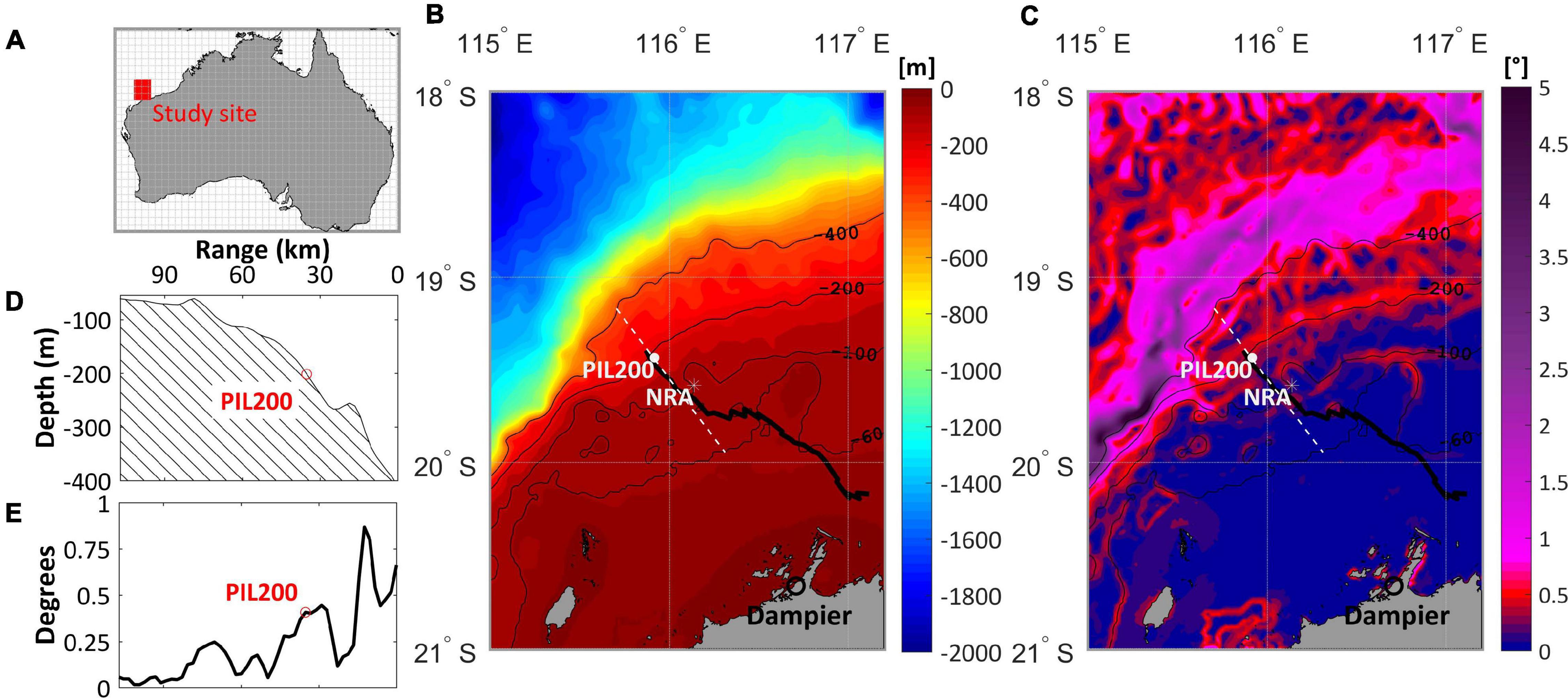
Figure 1. (A) The study site within the Australian North West Shelf. (B) Bathymetry, mooring station (PIL200), glider track (black line), and the North Ranking-A (NRA). (C) The slope, (D) bathymetric cross-section and (E) the related cross-sectional slope (in degrees).

Through analysis of satellite imagery, Baines (1981) was the first to identify internal tide structures on the NWS, but the use of hydrographic data on the investigations was pioneered by Holloway (1983a). The data set used by Holloway (1983a) was obtained from the continental shelf off Dampier as part of a measurement program associated with the exploitation offshore resources at the North Ranking-A (NRA; latitude 19.61°S, longitude 116.141°E) oil and gas platform (Figure 1B). Since then, a number of studies related to internal tides have been reported in the vicinity of NRA. The present study is also located in this region.

The generation region of internal tides within the study area has been identified to be in depths between 400 and 600 m, near critical slopes (Figures 1C,E) ∼70 km offshore from NRA, and ∼120 km along the slope (Craig, 1988; Holloway et al., 2001; Lim et al., 2008; Van Gastel et al., 2009). At NRA, where the local water depth is 123 m (Figure 1B), Holloway (1987) identified shoreward propagating first baroclinic mode (mode-one) semidiurnal tidal bores with diurnal inequalities. These waves produced frontal hydraulic jumps up to 60 m in the isotherms that were frequently but not always accompanied by ISWs. In spite of the sharpness of the measured bores, breaking and mixing events were not observed. Few studies to date have considered the internal wave field in the vicinity of NRA during the winter months. For example, Van Gastel et al. (2009) briefly characterized the winter internal wave field being weak and governed by waves of elevation.

The Australian NWS is subject to strong seasonality in wind forcing due to the action of the Australian monsoon. Here, the wind field varies from southeast trade winds (southeast monsoon) during the austral winter to south-west monsoon during the austral summer (Wijeratne et al., 2018). Winds usually have an alongshore component along the shelf in December-February. By March, winds drop to almost zero and during May to August they blow offshore. March and September are two monsoon transition periods when winds are weak and variable in direction. From October to November, alongshore southwesterlies are the dominant wind direction (Bahmanpour et al., 2016). The deepening of the thermocline from summer to winter is associated with southeasterly (offshore directed) trade winds become dominant. The major boundary current in this region, the Holloway Current, flows all year along the shelf edge (∼200 m depth contour) but is strongest during early winter months (Bahmanpour et al., 2016; Wijeratne et al., 2018). During the winter months there is strong cooling of the inner shelf regions that result in dense shelf water cascades (Mahjabin et al., 2020).

The NWS is mostly composed by carbonate sediments (Jones, 1970; Porter-Smith et al., 2004; Belde et al., 2017), ranging from 60 to 100% of the total weight of all samples evaluated by McLoughlin and Young (1985). These authors defined sedimentary provinces characterized by sand sediments at the shelf and muds at the upper slope, with a transition zone of intermediate composition between the two, which covers the region in the vicinity of the shelf break (nearby NRA).

Data Sources and Analysis

Field measurements were collected during September 2013 as part of Australian Integrated Marine Observing System (IMOS), which included (1) an oceanographic mooring (PIL200) located at 206 m depth, nominally on the upper slope; and, (2) an ocean glider transect across the shelf/slope (Figure 1B). The mooring consisted of a bottom mounted upward looking Acoustic Doppler Current Profiler (ADCP) and thermistors through the water column.

The Teledyne Workhorse 150 kHz Quartermaster series ADCP was configured to collect data at 10 m vertical bins, 5 min averages of 2.14 s interval pings. Details of sensor depths and sampling intervals for temperature sensors are available in the Supplementary Table S1 whist the locations of the moorings on a bathymetric cross section calculated from the ETOPO 1-arc min global relief model (ETOPO-1) are presented on Figure 1D.

Time series of temperature and salinity were linearly interpolated through vertical resolution of 1 m at each time step, following the method used by Van Gastel et al. (2009) to study ISWs near NRA. Since stratification in the study region was characterized by continuous gradients rather than by a two-layer structure, the interpolated field produced a reliable database to compute the depth variations for each isotherm. In addition, since temperature is the dominant parameter controlling density variations in the region (Holloway, 1987; Van Gastel et al., 2009), isotherms represented isopycnals in the analysis of the internal wave field. This approximation is generally assumed in observational studies undertaken on the NWS (e.g., Holloway, 1983a, 1984, 1987, 1994; Holloway et al., 1997, 2001; Van Gastel et al., 2009).

The time series data were subject to QA/QC flags defined by IMOS to remove spurious data from raw observations. For the velocity field, it meant the appearance of a gap in depths shallower than 28 m due to side-lobe effects. Another vertical gap of 9 m near the bottom was due to the ‘blind spot’ beneath the ADCP (combination of blanking distance and ADCP location as it had to locate above the acoustic release). Subsequently, the directions of the velocity field were rotated to compute the cross-slope (U) and along-slope (V) components. The onshore, eastward and upward directions were defined as positive.

The cross shelf measurements were taken by a Teledyne Webb Research Slocum Electric Glider operated by the IMOS Ocean Glider facility located at The University of Western Australia. The Slocum Glider for this experiment collected data (temperature, salinity, density, fluorescence, suspended sediment and dissolved oxygen) from the surface to ∼2 m above seabed to a maximum depth of 200 m with mean horizontal speed of 25 km per day (Pattiaratchi et al., 2017). Ocean gliders are autonomous vehicles that use a buoyancy engine for forward momentum moving to the target destinations to navigate their way to a series of pre-programmed waypoints using GPS, internal dead reckoning and altimeter measurements. The gliders were equipped with a Sea-Bird Scientific pumped CTD (conductivity–temperature–depth) sensor, a WETLabs BBFL2SLO 3 parameter optical sensor (which measured chlorophyll fluorescence, colored dissolved organic matter, and volume backscatter coefficient – VBSC at 660 nm), and an Aanderaa oxygen optode. However, only CTD and VBSC data are presented in this paper. All the sensors were sampled at 4 Hz, which yielded measurements every ∼ 7 cm in the vertical. The maximum duration of the descending (ascending) path was 22 min (18 min) on the vicinity of PIL200 and 6 min in water depths of 62 m.

IMOS data streams are provided in NetCDF-4 format with ocean glider data files containing metadata and scientific data for each glider mission. Subsequent to the ocean glider recovery, all the data collected by the glider are subject to QA/QC procedures that include a series of automated and manual tests (Woo, 2017). To maintain data integrity all of the sensors (CTD and optical sensors) are returned to the manufacturers for calibration after a period 365 days in the water. The Sea-Bird Scientific SBE 41CP pumped CTD sensor on the Slocum gliders is the same as those mounted on Argo floats and achieve temperature and salinity accuracies of ±0.002°Celsius and ±0.01 salinity units, respectively. In addition to the IMOS’s quality control flags, we considered spurious values external to an envelope of 3 standard deviations from the average of a 6 s moving window. This window was extended to a 2 min in the evaluation of the VBSC field due to its large number of spikes. Then, the series were linearly interpolated to a sample interval of 2 s.

Tides were delayed by T_B = (distance from the isobath of 400m)/c₀ in order to provide the correction that represents the barotropic scenario that generated the internal tides for the region, where $c_0=\sqrt{g^{\prime }{h}_1{h}_2/(h_1{h}_2)}$ is the phase velocity of the long-wave and g′ = g(ϱ₂−ϱ₁)/ϱ₂ is the reduced gravity due to a stratified water column. These parameters assume a two-layered vertical structure, where h₁ and h₂ are, respectively, the upper and lower layers thicknesses at PIL200.

Environmental Parameters

A direct way to characterize the oceanographic conditions responsible for particular nonlinear characteristics of the incident internal wave is to calculate the coefficients that parameterize nonlinear steepening (α) and dispersion (β) effects on the KdV equation. Holloway et al. (1997) used the KdV to model the cross-slope evolution of a sinusoidal long internal tide on the proximity of NRA, addressing how changes in α and β impacted the computed waveforms.

In the context of a two-layered vertical structure α and β are simply

${\mathrm{\alpha }}_0={\displaystyle \frac{3c_0}{2}}{\displaystyle \frac{h_1-h_2}{h_1{h}_2}},{\mathrm{\beta }}_0={\displaystyle \frac{c_0}{6}}{h}_1{h}_2(1)$

These quantities are commonly referred as environmental parameters since they are external to the waveform (e.g., Cai et al., 2008; Walter et al., 2016). However, assuming the full-nonlinear solution that includes the background shear current (Shi et al., 2009) and a continuous stratification, the KdV parameters are given as (Holloway et al., 1997):

$\mathrm{\alpha }=\left({\displaystyle \frac{3}{2}}\right){\displaystyle \frac{{\int }_{-H}^0{(c-U)}^2{(d\mathrm{\Phi }/dz)}^3\mathit{d}z}{{\int }_{-H}^0(c-U){(d\mathrm{\Phi }/dz)}^2\mathit{d}z}},$

$\mathrm{\beta }=\left({\displaystyle \frac{3}{2}}\right){\displaystyle \frac{{\int }_{-H}^0{(c-U)}^2{\mathrm{\Phi }}^2\mathit{d}z}{{\int }_{-H}^0(c-U){(d\mathrm{\Phi }/dz)}^2\mathit{d}z}}(2)$

Where z is the vertical coordinate, c the long-wave propagation speed and U(z) the background shear velocity. The vertical structure function Φ(z) is determined by the eigenvalue problem in terms of integrals of the long-wave limit (e.g., Stastna and Lamb, 2002)

${\displaystyle \frac{d}{dz}}\left[{\left(c-U\right)}^2{\displaystyle \frac{d\mathrm{\Phi }}{dz}}\right]+N^2\left(z\right)\mathrm{\Phi }=0,\mathrm{\Phi }\left(-H\right)=\mathrm{\Phi }\left(0\right)=0(3)$

The above equation is known as the Taylor–Goldstein (TG) equation. The TG theory is incorporated by the Dubreil Jacotin Long (DJL) equation, which have been applied to resolve mode-one propagating waves of permanent form up to the onset of breaking (Walter et al., 2016). Here, we used the MATLAB packet Dubreil-Jacotin-Long Equation Solver (DJLES) https://github.com/mdunphy/DJLES/ (Dunphy et al., 2011) in order to obtain Φ(z) and c, as we were interested in only the vertical structure and phase speed of mode-one waves intrinsic to the local environment. For comparison, such intrinsic properties were also computed following the methodology presented by Klink (1999), which does not consider background currents.

The Brunt-Väisälä frequency (or buoyancy frequency) N is required to resolve the TG equation

$N^2\left(z\right)=-{\displaystyle \frac{g}{\mathrm{\rho }\left(z\right)}}{\displaystyle \frac{d\mathrm{\rho }\left(z\right)}{dz}}(4)$

Where g and ρ are, respectively, the gravitational acceleration and potential density. In order to evaluate α and β in equations (2), Holloway et al. (1997) solved the TG equation over 10-day and 4-day means. Later, Holloway et al. (2003) analyzed the same series over 12-h means and elucidated that the results were affected by perturbations in the semi-diurnal frequency. For this reason, in this study, the tidal internal wave signal was smoothed out from the series using a low-pass-36-h Lanczos filter in order to obtain the profiles of U(z) and N(z) computed over 2 day section averages.

The vertical limit of integration of equation (2) was not covered by the sensor array. We approached this issue by first incorporating OSTIA daily averaged sea surface temperature (SST) at 3-arc min (∼ 5.5 km) resolution to the temperature field. Near the bottom, however, the vertical gaps were small (∼ 5 m), thus we simply replaced it by the nearest measurement. The same approach was applied over the surface gaps of salinity and U fields. Since measurements carried on nearby the depth of 27 m were seen within the limits of the surface mixed layer, similar characteristics are expected up to the surface.

Additionally, the dimensionless form of equations (2) was applied on the determination of an environmental breaking criterion for the internal tides in the region

$\delta =\left({\displaystyle \frac{\mathrm{\beta }}{mean\left(\mathrm{\beta }\right)}}\right)/\left({\displaystyle \frac{\mathrm{\alpha }}{mean\left(\mathrm{\alpha }\right)}}\right)(5)$

Baroclinic Current and Energy

The horizontal direction in which the internal waves propagate was estimated by the orientation of the semi-diurnal (M₂ + S₂) baroclinic ellipses but with an ambiguity of 180^o (Holloway, 1984), i.e., the same direction of the linear internal tide was assumed.

Estimates of the baroclinic components of the current (U_C and V_C) were obtained from the total velocity with the barotropic components removed (Holloway et al., 2001; Xie et al., 2015). With this, we turn the focus on baroclinic motions associated with internal waves. It should be mentioned here that U_C and V_C jointly incorporate the fluid particle velocities due to breaking dynamics (Vlasenko and Hutter, 2002). It should be noted that V_C is disregarded in the dynamical analysis associated to the observed waveforms. This is on the assumption that the breaking of a nonlinear internal tide is a phenomenon of cross-slope nature, given the influence of the slope on the shoaling wave. In addition, numerical studies that resolve breaking waves generally apply a two-dimensional model (e.g., Vlasenko and Hutter, 2002; Aghsaee et al., 2010; Bourgault et al., 2014), which supports the idea that most theories exist in the cross-slope frame.

The energetics of the internal wave field was examined through the Welch’s power spectral density (PSD) analysis, considering the depth variation of the isotherm most representative of the thermocline sampled at 2-min interval with 16 degrees of freedom at the 95% confidence interval. Sensors with sampling intervals higher and lower than 2 min were, respectively, resampled and not considered to obtain the temperature field. The comparison between different PSD was possible due to the “normalization” through standard deviation. In addition, due to the degrees of freedom the resolution at low frequencies was small; thus the focus in this paper is on the description of moderate and high-frequency variations.

The spectral shapes of each section were also considered in terms of the fall-off rate, defined conformably to the power-law distribution 1/f^x, with the exponent x indicating the slope of the curve and f the considered frequency band (Freeman and Zhai, 2009). The PSDs together with theoretical analysis associated with the observed kinematics are evidences of the main characteristics of the internal wave field in each 2-day section.

Turbulent Mixing

Quantifying the rate of turbulent mixing (or strength of mixing) in a fluid with a stable density gradient is central to the understanding of the transport of heat, salt and material. Following the seminal work of Thorpe (1977) and Dillon (1982), vertical density overturns in an otherwise stably stratified fluid is commonly used to indirectly estimate the dissipation rate of turbulent kinetic energy ε. This method assumes a linear correlation between the Thorpe length scale L_T, an observable estimate of the scales of vertical overturning, and the Ozmidov length scale L_o = (ε/N³)^1/2 (e.g., Lien et al., 2012; Mater et al., 2015):

$\epsilon \sim L_O^2{N}^3={(0.8L_T)}^2{N}^3(6)$

L_T was computed from the 2 m root-mean-square of the Thorpe displacement, which in turn relied on the misfit between the observed isopycnal depth and the sorted isopycnal depth (Wijesekera and Dillon, 1991). The Thorpe displacement was initially calculated from downcast glider profiles. The lower limit of each profile was reduced by 5 m in order to avoid spurious jumps of displacement near the seabed. The L_T for the period was of the order of tens of meters, thereby the turbulent eddies were large enough to have their effect felt by the array of sensors on PIL200. Therefore, L_T was also computed for the interpolated fields of 1 m at each time step.

On the Monterey shelf, Carter et al. (2005) observed that ε ranged from 10^–10 to 10^–5 W Kg^–1 under the effect of shoaling ISWs. Klymak and Moum (2003) estimated ε of 10^–6 W Kg^–1 associated to internal waves of elevation surging over Oregon’s continental shelf. On higher scales of turbulence, Wesson and Gregg (1994) observed mixing at Camarinal Sill in the Strait of Gibraltar exceeding 10^–2 W Kg^–1. On that account, ε < 10^–9 W Kg^–1 was set as the noise level in this study.

Ocean Glider Profiles

Glider observations of VBSC provided information on suspended material concentrations. A cross-shelf view of the environmental consequences of the internal wave field during the austral winter was inferred from the cross-shelf fields of temperature, N and VBSC. Additionally, qualitative comparisons with the glider mission of February 2014 was incorporated to the analysis mainly in order to elucidate implications of the late winter vertical structure for vertical mixing, resuspension and transport of water and material.

By assuming the quasi-static model of a planar glider, where W_total is the total downcast velocity and W_mec is the mechanical downcast velocity (Merckelbach et al., 2010), we estimated the water vertical velocity W_gld

$W_{gld}=W_{total}-W_{mec}(7)$

Considering that turbulent and internal wave disturbances were small far from the surface and the stratified portion of the water column W_mec was computed as the mean downcast velocity along the entire deployment between depths of 15 to 40 meters. Furthermore, since the maximum duration of the profiles was 22 min, semi-diurnal internal tidal dynamics were expected to be satisfactorily resolved.

Results and Discussion

Linear Internal Tides

We computed the long-wave phase velocity of _c0 = 0.77 m s^–1, resulting in a delay of T_B≅ 13 h. The latter provided the correction that approximated tides to the scenario that generated the observed internal waves. The corrected tides must be carefully interpreted as large differences are expected between the barotropic current where the observations were taken (PIL200) and at the likely generation region (Holloway et al., 2001). On average, an ebb tidal amplitude of 0.87 m and its corresponding cross-slope barotropic current of 0.1 m s^–1 (Figure 2A) produced shoreward internal tides that encountered undisturbed isothermal surfaces on PIL200, represented by the low-pass-36-h filtered temperature field (Figure 2B).

FIGURE 2

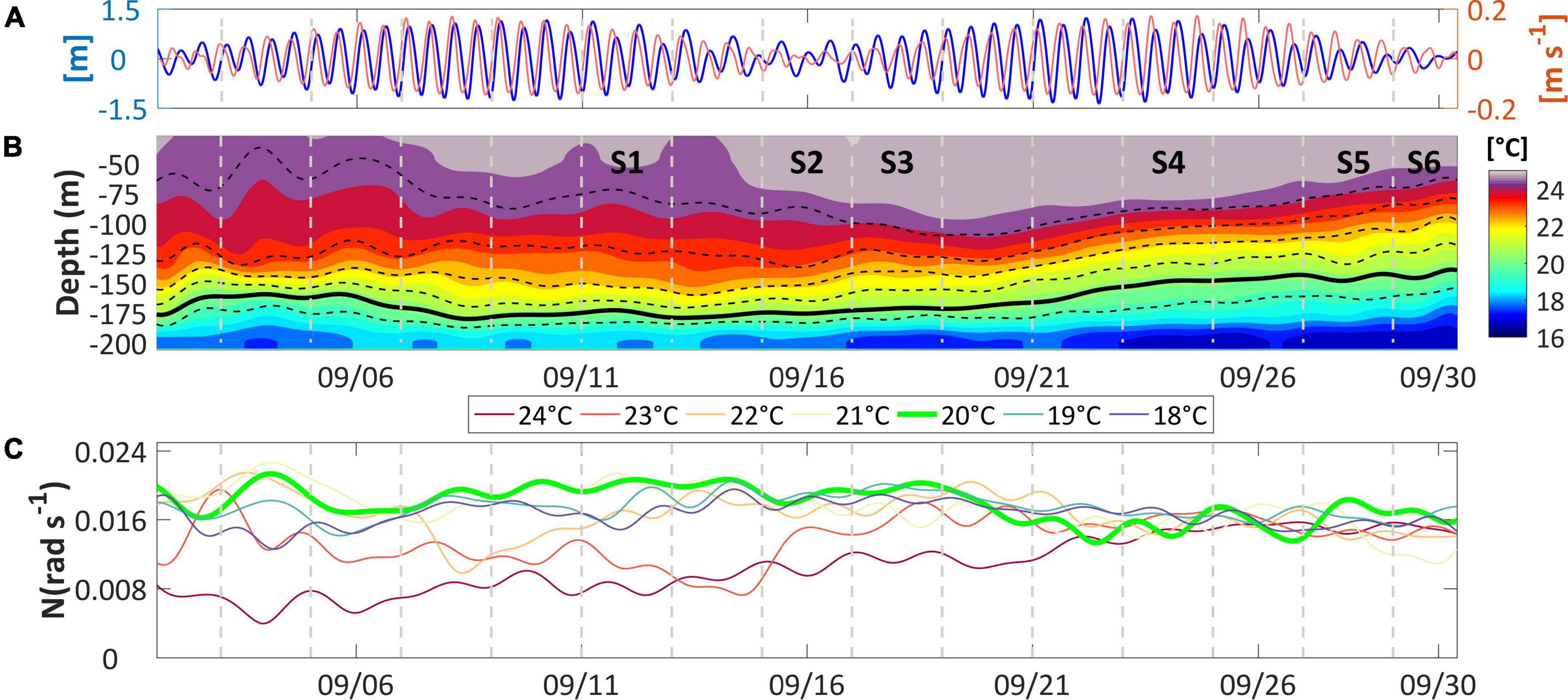
Figure 2. (A) The tidal amplitudes (left axis) together with the tidal cross-slope barotropic currents (right axis) on PIL200, delayed of ∼ 13 h to represent the generation scenario. (B) The subinertial (low-pass-36-h filtered) temperature field, displaying the depth of isotherms from 19 to 24°C, and the 2-day segments (vertical gray dashed lines) which define the time intervals of interest (S1 to S6). The thick black line marks the 20°C isotherm. (C) The brunt–Väisälä frequencies corresponding to these isotherms.

The mean orientation of the semidiurnal (M₂ + S₂) anticlockwise baroclinic ellipses, related to a reference approximately parallel to the shelf edge, was 270° (Supplementary Table S2), indicating that linear internal tides were strongly shoreward propagating. In addition, the corresponding baroclinic tidal currents were minimum at mid-depth (∼109 m), whereas the maximum was near surface and close to the bottom. These, together with the phase jump of ∼10° near mid-depth accounted for the mode-one nature of the internal wave field (Liao et al., 2011).

Environmental Conditions

The undisturbed temperature field and the isothermal surfaces from 19 to 24°C are presented in Figure 2B. Analyses of the buoyancy frequencies (N) associated with the depth of these surfaces indicated the 20°C isotherm (Figure 2B, thick solid line) as the best representation of the thermocline, since it displayed the maximum values for majority of the period (Figure 2C, thick green line). Therefore, its average of 0.0179 rad s^–1 (∼ 6 min) is the approximation for the local buoyancy frequency (N_l). The 2-day defined segments analyzed here (S1 to S6; Figure 2B) were selected due to the number of significant and interesting features, which were consistent with particular dynamic stages predicted by the internal wave breaking theory.

The distribution of the buoyancy surfaces revealed that the stratification was characterized by continuous gradients rather than by a two-layer structure, remarkably after the 21^st September, when the surfaces attained similar values (Figure 2C). This was more directly evidenced throughout the profiles of buoyancy at the time intervals named S4, S5 and S6 (Figure 3A, black solid lines). In such cases, there was no single peak in buoyancy around the depth of the thermocline, but a broad layer of near-uniform buoyancy approximately between the depths of 80 and 190 m. This layer dramatically changed at the segments S1, S2 and S3 (Figure 3A, black solid lines), becoming narrower, deeper and stronger. In addition, the buoyancy profiles became attenuated from the bottom of this layer all the way to the surface. Therefore, it is reasonable to argue that the destabilization of the stratification in these segments could possibly result from the onset of an efficient mechanism in dissipating the internal tide and providing energy for vertical mixing (Holloway et al., 1997).

FIGURE 3

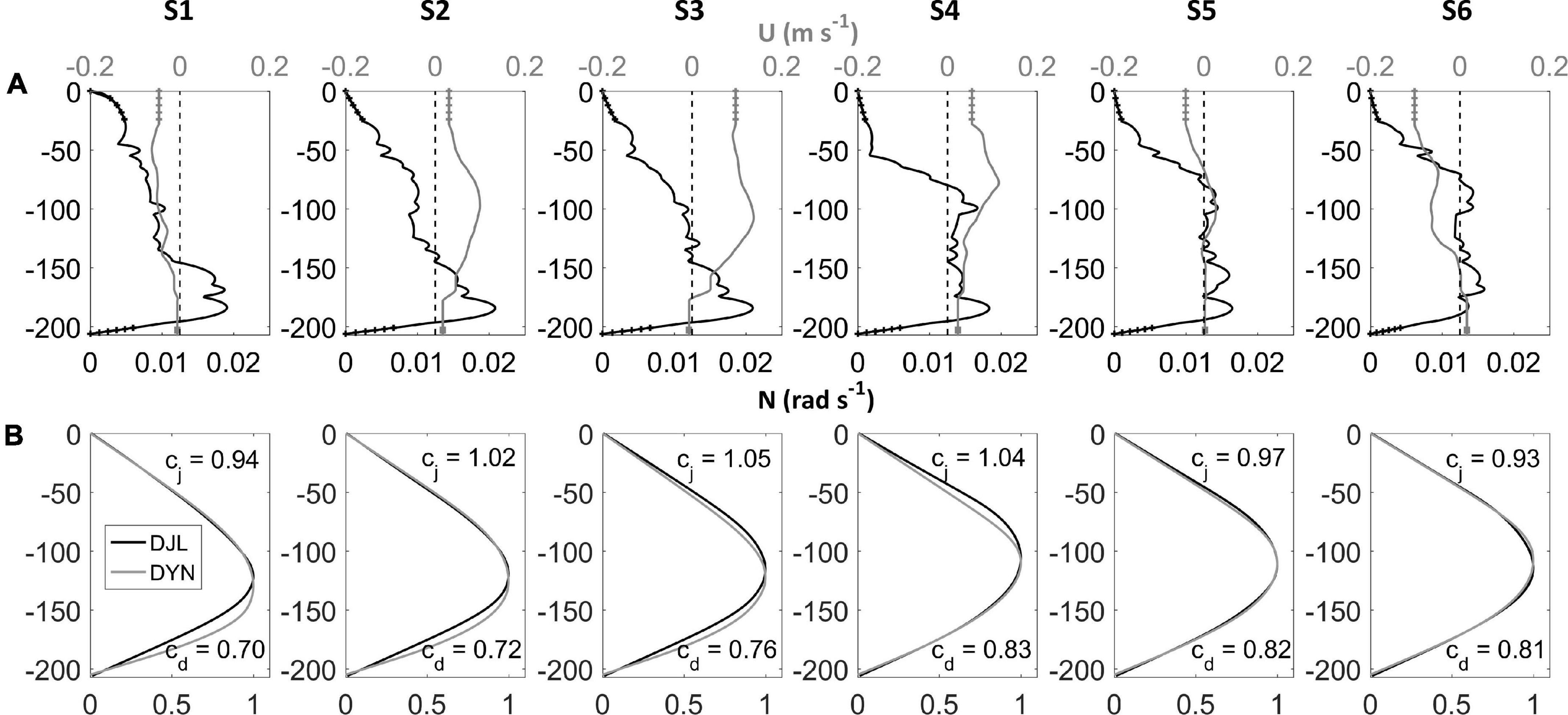
Figure 3. (A) Profiles of Brunt-Väisälä frequency N (rad s^–1, black) and background current U (m s^–1, gray) averaged for each relevant 2-day segment (S1 to S6); the hatched vertical segments of each profile signalizes the limits not covered by the deployed arrays of sensors, and the gray vertical dashed line marks the zero m s^–1. (B) The vertical structure function Φ(z) and phase velocity values for the first baroclinic mode determined through the full-nonlinear Dubreil-Jacotin-Long method (respectively, DJL and c_j) and without background currents (DYN and c_d).

Although the normalized vertical structure function Φ(z) obtained through the full-nonlinear DJLES was similar to the one without background currents (Figure 3B, respectively, DJL and DYN), the mode-one phase speed obtained through the first (c_j) was higher in comparison to the second (c_d).

Although both continuous N profiles and background currents were deterministic in computing α and β, the corresponding parameters α₀ and β₀ behaved similarly (Figures 4A,B). For instance, the transition from the time intervals S1| S2| S3 (group-1) to S4| S5| S6 (group-2) was marked by the decline of nonlinear steepening and the rise of dispersion. This allowed for the dimensionless parameter being δ < 1 for the former and δ > 1 for the latter (Figure 4C), considering both full-nonlinear and two-layered solutions. This indicates distinct environments governing aspects of the nonlinear wave field between group-1 and group-2.

FIGURE 4

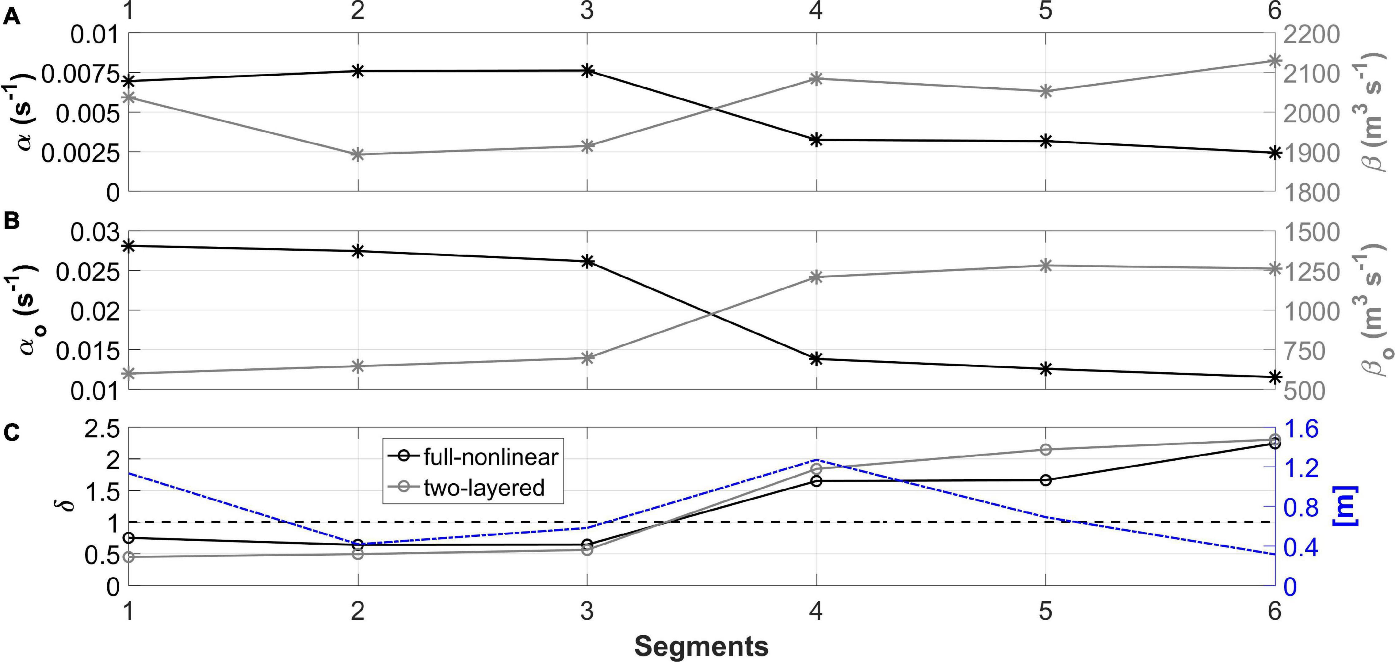
Figure 4. (A) The coefficients that parameterize nonlinear steepening α (black) and dispersion β (gray) effects on PIL200 through the full-nonlinear method calculated for each relevant 2-day segment (S1 to S6). (B) The same estimation through two-layered solutions α₀ (black) and β₀ (gray). (C) The dimensionless form relating the environmental parameters δ (black) and δ₀ (gray) and the averaged ebb tidal amplitudes from the adjusted generation scenario (delayed of ∼13 h; blue); the horizontal dashed line marks the criterion of dimensionless parameters equal the unit.

A higher α(β) existed under prevalence of onshore (offshore) currents, as evidenced considering the response of S1| S2| S3 (Figure 4A) to changes in the background shear currents (Figure 3A, gray solid lines). In addition, α was maximum in S3, when the core of the onshore background current exceeded 0.13 m s^–1. This parameter was positive and always >0.0025 s^–1 and its maximum was 0.0075 s^–1. These values of α are considered to be strong, reason why we have intentionally left out the cubic and quadratic nonlinear steepening terms.

According to Holloway et al. (1997), similar values of α have been experienced by environments internal to the shelf break during late summer (March and April). In contrast, α₀ extrapolated by far the values estimated by Holloway and α (Figures 4A,B). At the same time, β₀ underestimated β. Therefore, these results suggest that the two-layered solutions do not accurately represent the competing nonlinear and dispersive effects given by the observed oceanic conditions. Therefore, we will take α, β and δ as defined by their full-nonlinear solutions in the subsequent sections.

Pre-breaking Waves

The theoretical consistency of the kinematics presented here and in Section “Post-breaking Waves” supported the grouping of time intervals as post-, S1| S2| S3 (group-1), and pre-, S4| S5| S6 (group-2), wave breaking. It should be noted that this matches the same two groups of segments presented in Section “Environmental Conditions” that computed similar values of the non-dimensional parameter δ, which was introduced as a criterion for breaking (δ < 1).

Among the observed packets of nonlinear internal waves in each 2-day segment (S1 to S6), only intervals (∼ 9 h) most consistent with characteristic dynamic stages predicted by the internal wave breaking theory were selected for analysis (Figures 5A,B). We have proposed a sequential progression throughout this analysis from the packet of the strongest suppression of nonlinear steepening by dispersion, toward the one of the strongest cumulative effect of nonlinear steepening. i.e., from S6 toward S4. In Section “Post-breaking Waves,” this progression was completed with S3, S2 and S1 incorporated to the analysis.

FIGURE 5

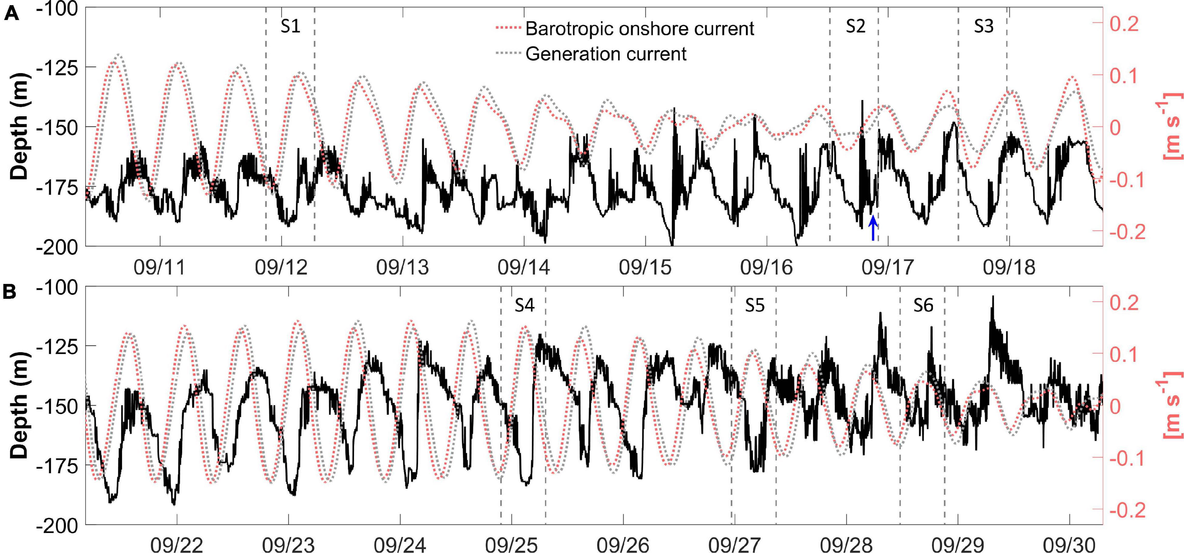
Figure 5. (A,B) Time series of depth of the 20°C isotherm (left axis) together with the tidal cross-slope barotropic currents (right axis) at the time of measurement and adjusted to the generation scenario (delayed of ∼13 h). The ∼ 9-h segments (vertical gray dashed lines) which define the most representative features within each section of interest (S1 to S6) are also shown. In S2, the blue arrow signalizes the presence of a separation in the back of the packet of turbulent boluses (referred in text).

In S6, the semidiurnal tidal bore was barely discernible at the 20°C isotherm (Figure 5B). From the hydraulic jump of ∼32 m backward (Figure 6A, T1 →), the rear shoulder of the long-wave gave way to a dispersive wave packet of short-period ISWs, mostly depression-like waves, but with evidence of second mode waves. From this jump forward (Figure 6A, ← T1), throughout the length of the long-wave trough and front shoulder, the ISWs became more elevation-like and the mode-two characteristics were more clearly depicted. Following the numerical results of Vlasenko and Stashchuk (2007), the very existence of a dispersive packet at the rear shoulder of the wave indicated that dispersion had sufficient time to balance nonlinearity and to suppress the formation of an energetic rear face bore. i.e., before the wave arrived in S6, an important part of its energy was likely transferred to the frequency bandwidth of ISWs. Indeed, the narrowness of the PSD about the local buoyancy frequency N_l during this period (Figure 7A) implied that the rate at which energy was made available to ISWs was significant (Boegman et al., 2003). Further noteworthy is that the spectra experienced a fall-off rate enhancement to σ⁻⁶ just after N_l, i.e., dissipation was stronger after this frequency, suggesting that the train of ISWs played an important role in the energy dissipation of the internal tide.

FIGURE 6

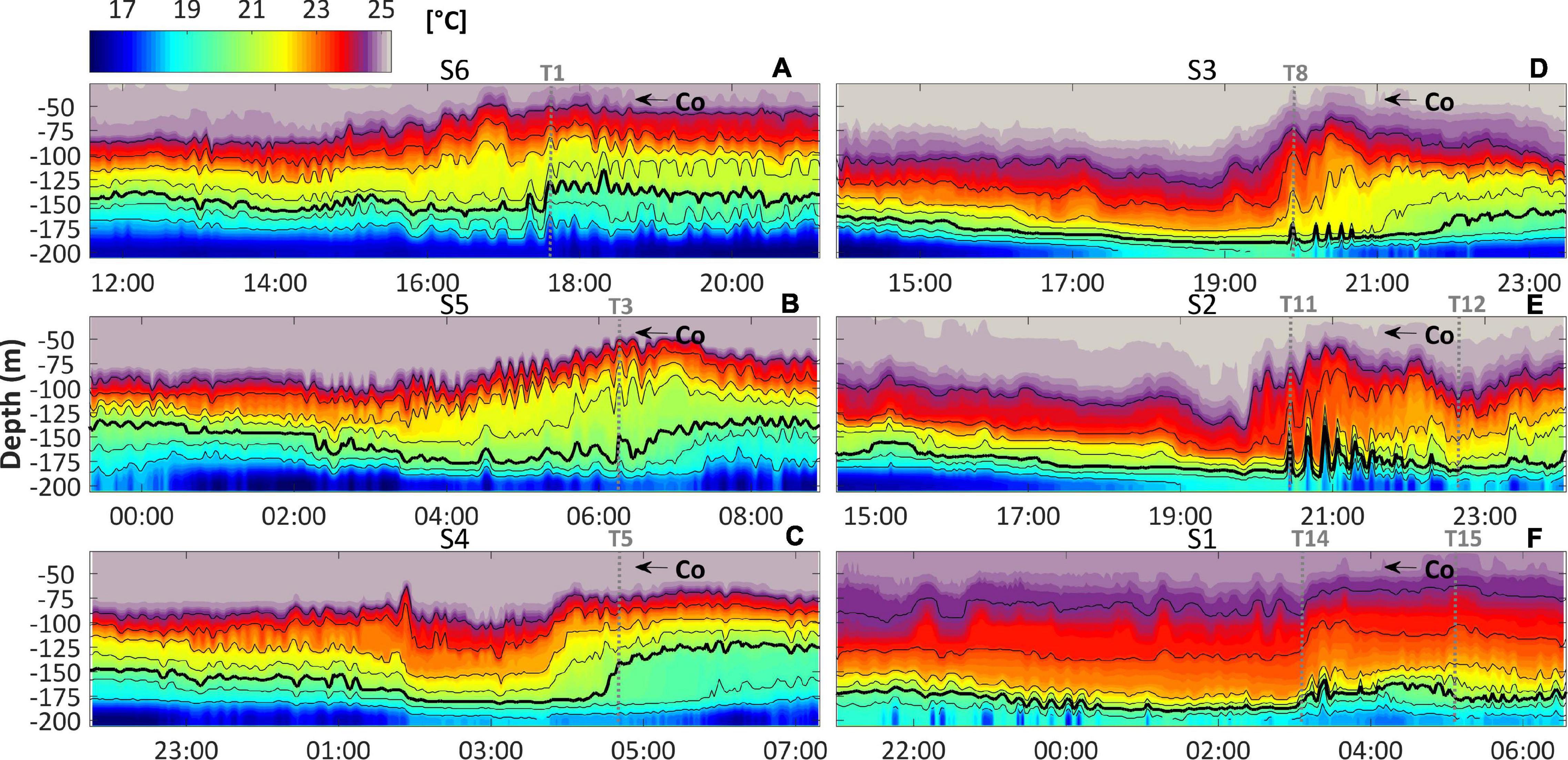
Figure 6. (A–F) Temperature field calculated for the most representative feature within each relevant 2-day segment. The depths of relevant isotherms from 18 to 24°C are displayed and c_o indicates the shoreward wave propagation direction. The gray vertical dotted lines mark features referred in text.

FIGURE 7

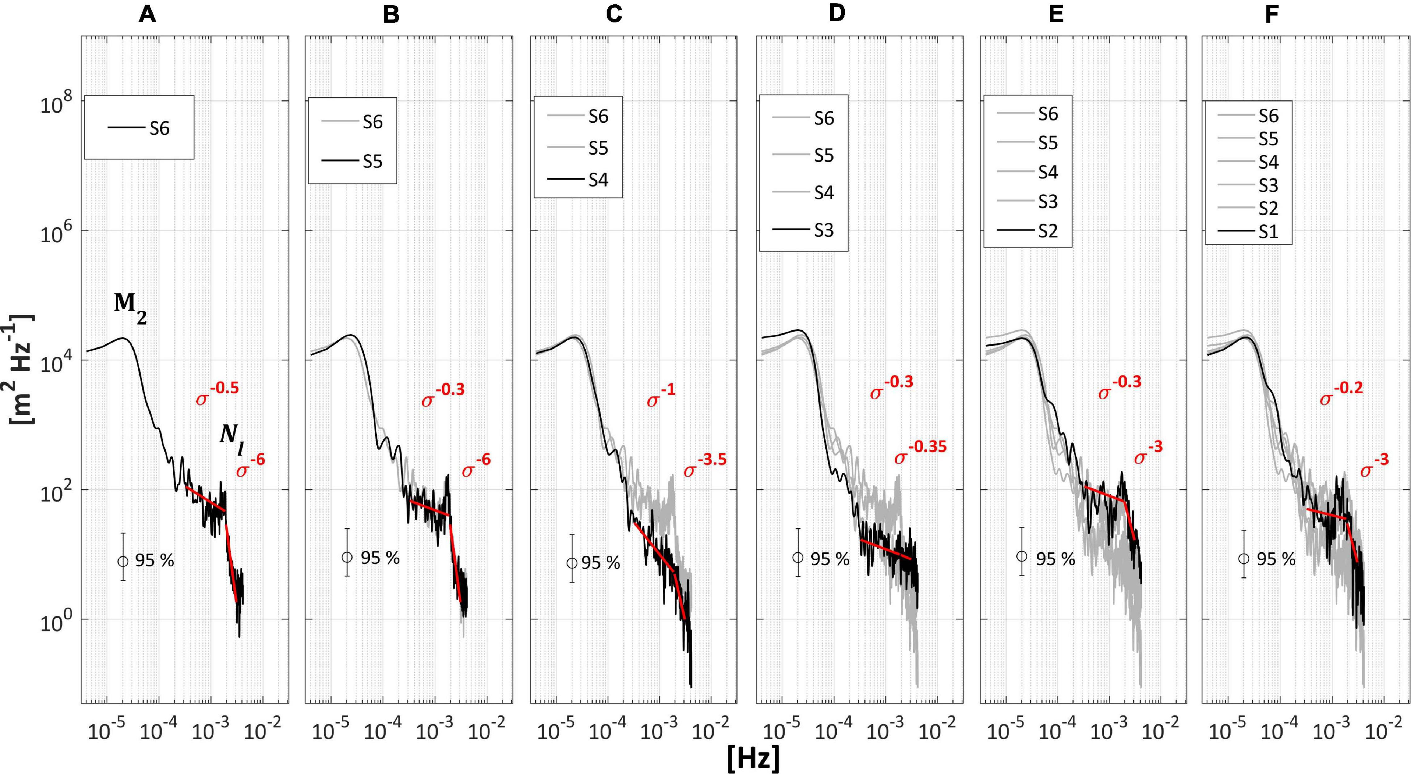
Figure 7. (A–F) Welch’s power spectral densities (PSD) calculated for each relevant 2-day segment on PIL200 within a confidence interval of 95%. The fall-off rates are addressed from 1-h to the local buoyancy frequency (N_l) and from N_l to 4-min.

A region of downslope oriented baroclinic currents developed in the lower layer along the wave trough and front shoulder (Figure 8A, ← T1), reaching magnitudes up to −0.24 m s^–1. Several studies have shown that such a flow is generated by fluid escaping beneath the flattening front shoulder of a shoaling wave of depression (e.g., Helfrich, 1992). On the other hand, the upslope counterpart of the flow has been related with a steepening rear shoulder, which alone would act to move the location of maximum baroclinic currents from the wave center toward the rear face (Aghsaee et al., 2010). In S6, however, the maximum speeds were maintained near the center of the long-wave (Figure 8A, T2 ↔ T1), presenting magnitudes up to 0.25 m s^–1, with offshore currents above and below. This three layer pattern during the time of the internal bore may be related to the presence of mode-two waves (Small et al., 1999). As shown in laboratory and numerical experiments (e.g., Helfrich and Melville, 1986; Lamb and Warn-Varnas, 2015), mode-two waves may be generated by shoaling mode-one waves of depression undergoing instabilities, which goes from interfacial shearing to wave breaking.

FIGURE 8

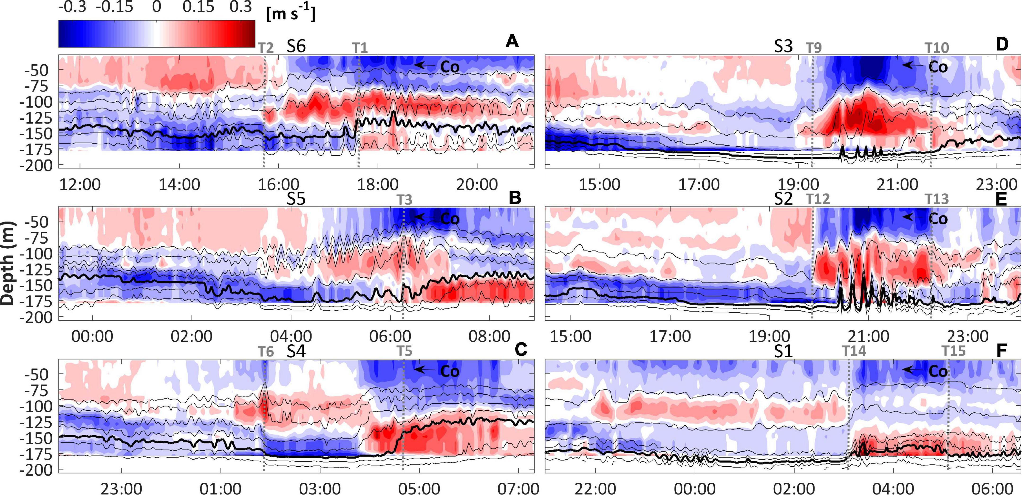
Figure 8. As in Figure 6, but for (A–F) baroclinic onshore velocity field.

The three layer structure of wave-induced currents observed in S6 imposed a relevant top to bottom gradient of velocity near the center (Figure 8A, T2 ↔ T1), which led to the development of important shear-driven instabilities expressed in terms of the short-period events of Ri < 0.25 (Figure 9A, T2 ↔ T1). Despite of that, the resulted turbulent eddies (Figure 10A, T2 ↔ T1) were not necessarily driven by shear. It was possibly be related to intrinsic nonlinear aspects of the internal tides or ISWs that shoal in this region (Holloway et al., 2001). Some turbulence bursts exceeded 10^–3 W Kg^–1 nearby the rear jump (Figure 10A, T1) which is six orders of magnitude greater than that in the typical open ocean (Lien et al., 2012). Consequently, these eddies were strong enough to erode stratification and form patches of mixed fluid at the depth of ∼125 m (Figure 11A, T2 ↔ T1). We will refer to this layer as “interior mixed layer” in order to draw a clear distinction with the boundary mixed layers (surface and bottom). Notably, the interior mixed layer impacted the average buoyancy profiles in S6 (Figure 3A, black solid lines), forming a zone of reduced stratification close to its average depth. There were also evidence of wave-induced turbulent eddies in the lower layer, which ranged from 10^–9 to 10^–4 W Kg^–1, directly energizing the bottom boundary layer in the course of the long-wave (Figure 10A). As shown in laboratory and numerical experiments (e.g., Bourgault et al., 2014), this mechanism is known to provide favorable conditions for sediment resuspension.

FIGURE 9

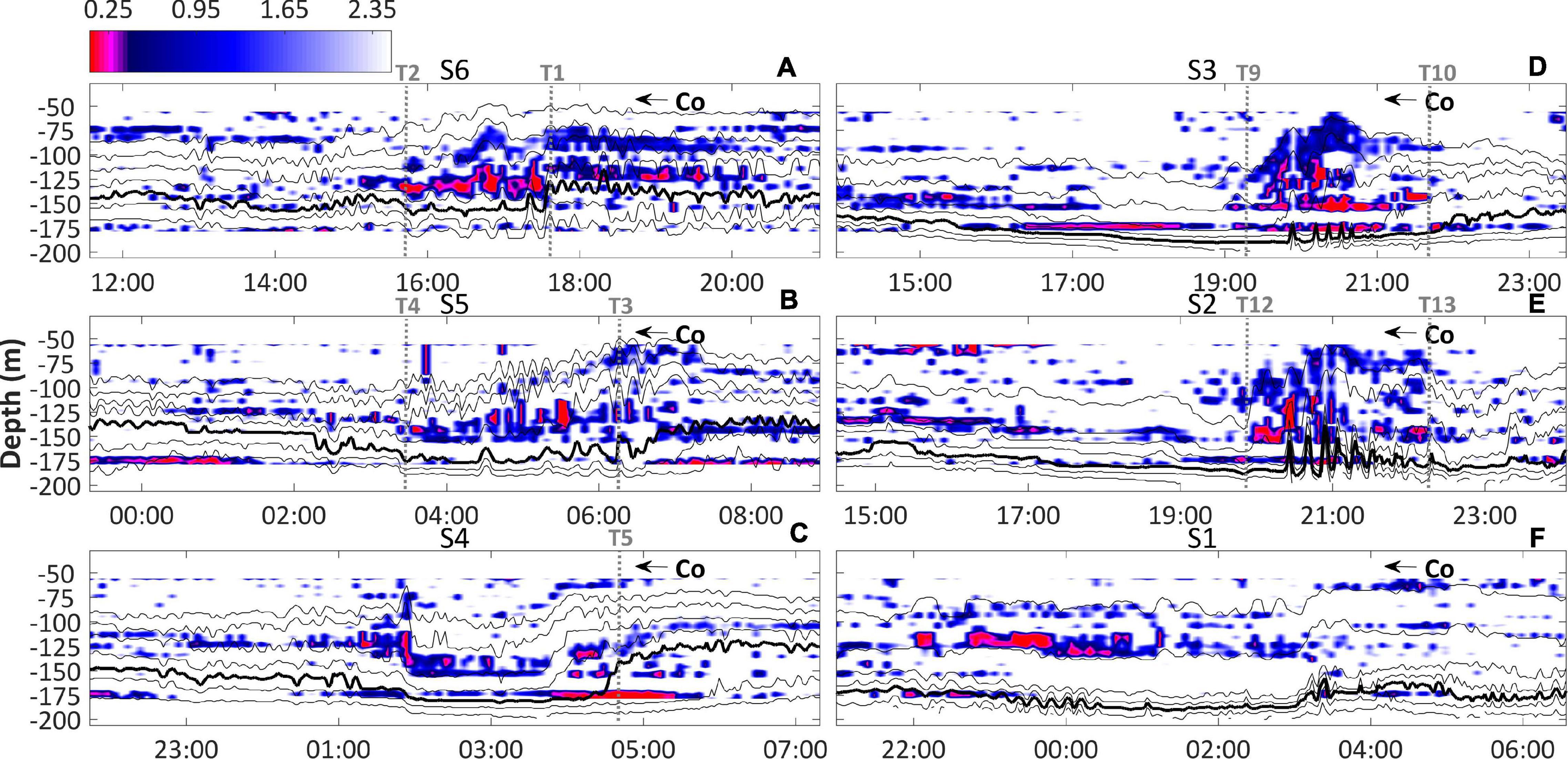
Figure 9. As in Figure 6, but for (A–F) non-dimensional Richardson number field.

FIGURE 10

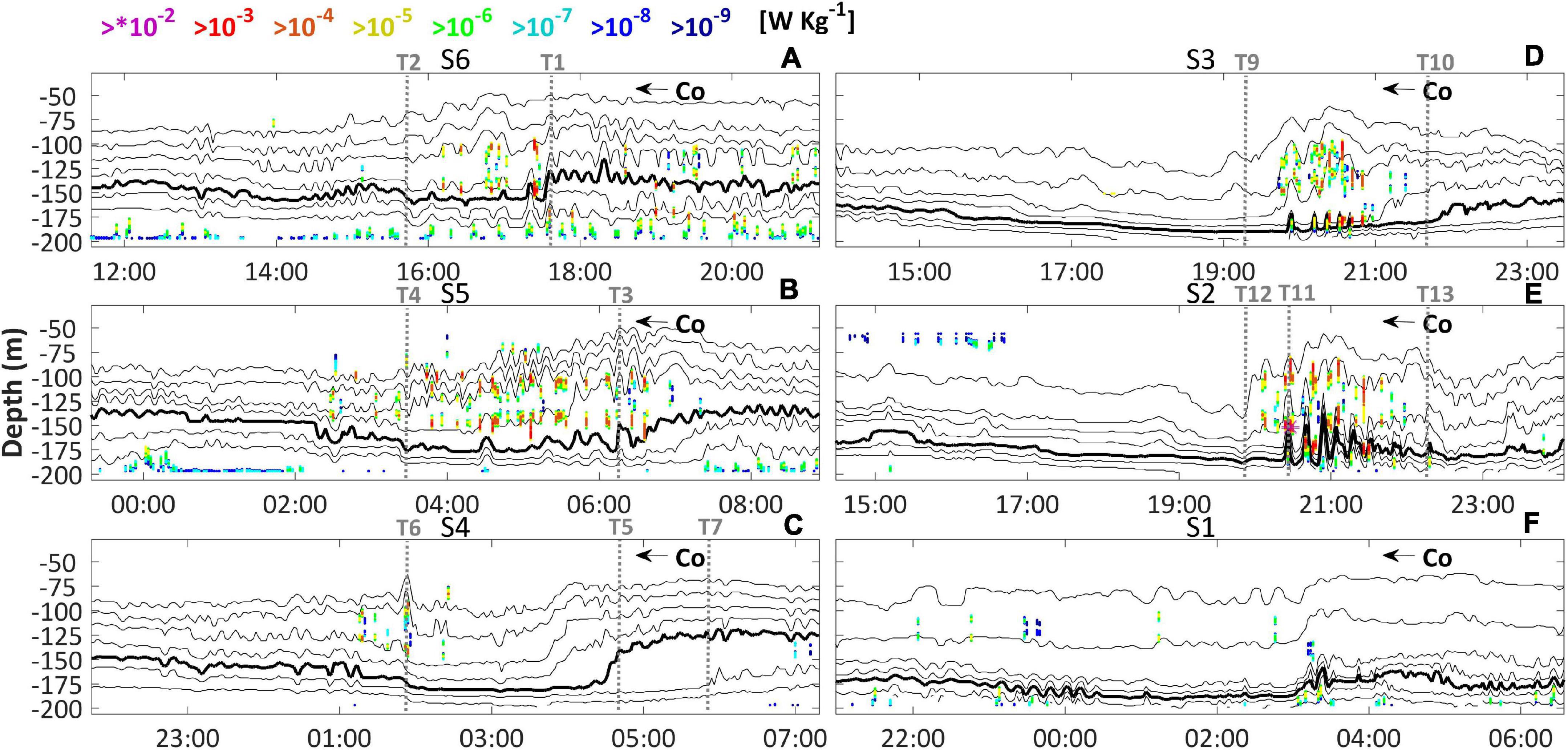
Figure 10. As in Figure 6, but for (A–F) rate of turbulent mixing field.

FIGURE 11

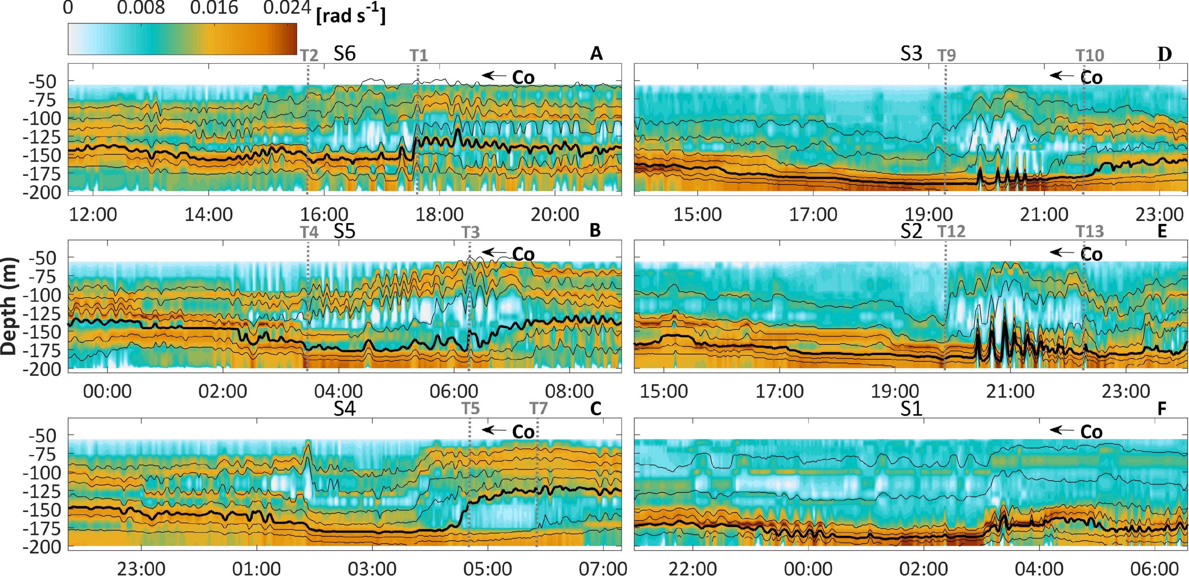
Figure 11. As in Figure 6, but for (A–F) buoyancy frequency field.

In essence, the kinematics in S6 was consistent with the environment of maximum δ (Figure 4C, solid black line), and the dispersive effects went harsh enough to scatter a significant amount of energy out of the tidal bore during its shoreward propagation from the generation site. It was not only under the effect of energy scattering that the tidal bore became suppressed. The average tidal amplitude during the ebb phase, delayed by ∼13 h to represent the generation scenario, was a minimum (0.3 m; Figure 4C, blue line), implying that just a weak pycnoclinic depression departed from the generation site and, consecutively as the depression moved onshore, a tidal bore of minimum amplitude was formed (Gerkema and Zimmerman, 2008). Due to the fact that the wave amplitude is directly proportional to its characteristic nonlinear steepening (Vlasenko et al., 2005), the tidal bore in S6 had further dispersive characteristics.

In S5, dispersion became less important as δ decreased (Figure 4C, solid black line), at the same time the ebb tide increased to 0.7 m (Figure 4C, blue line). The enhancement of the nonlinear effects by its steepening clearly defined a semidiurnal tidal bore at the 20°C isotherm (Figure 5B). However, instead of a hydraulic jump at the front, which dominated observations on the NWS edge in summer (e.g., Holloway, 1987), the long-wave disclosed a flattened front shoulder accompanied by ISWs that appeared to merge into a steep rear shoulder (Figure 6B, T3 →). Therefore, indicating that the setup of a rear face bore was on course (Chen et al., 2010). In such a case, the energy about N_l built sufficient energy to appear as a narrow peak amongst nearby frequencies (Figure 7B), possibly due to the more energetic tides associated with the wave genesis and the less dispersive environments it encountered during S5.

The kinematics associated with the tidal bore in S5 moved the location of maximum upslope oriented baroclinic currents from the wave center to the lower layer along its rear shoulder (Figure 8B, T3 →), thus checking on the consistency of the observed waves with theory (Aghsaee et al., 2010). Despite the reduction of the shearing instabilities near the center of the long-wave (Figure 9B, T4 ↔ T3) in comparison with S6, there was a complex picture of nonlinear undulations at the interior mixed layer that intensified the turbulent mixing throughout the center of the long-wave (Figure 10B, T4 ↔ T3), as well as the erosion of the stratification in this layer (Figure 11B, T4 ↔ T3).

In S4, whilst there was just a slight reduction of δ in comparison with S5 (Figure 4C, solid black line), the tidal amplitude that generated the propagating internal tides increased to 1.3 m (Figure 4C, blue line), the maximum for the period. Unlike in S6 and S5, cumulative effect of nonlinear steepening led the long-wave to become clearly non-symmetric as the front shoulder flattened and the rear shoulder steepened, displacing the 20°C isotherm ∼45 m upward and producing a well-defined rear face bore (Figure 6C, T5). This highlights the critical role that energy supplied to the system by barotropic tides may have in the study region.

The spectra in S6 and S5 differed crucially from the approximately monotonic fall-off rate outlined in S4 (σ⁻² on average; Figure 7C), which suggested a more straightforward transfer of energy from the long-wave into the turbulent scales. Hosegood and van Haren (2006) observed a similar rate of change associated to tidal bores near the generation site over the continental slope on the Faeroe-Shetland Channel. This necessarily implies similarities on the spectrum of tidal bores and rear face bores, which are due to the existence of both under the dominance of nonlinear steepening (α) in detriment of dispersion (β).

The occurrence of tidal bores or rear face bores in a particular location strongly relies on the sign of α. Holloway et al. (1997) have shown, through model and observations, that under late summer oceanic conditions on the NWS, tidal bores were formed as the wave moved onto the slope under weak β and strong negative α (h₁ < h₂). Further onshore, but yet before the turning point where h₁ = h₂, which is the site of weakest α, energy started to cascade into trains of ISWs due to the dominance of dispersive effects. It was only over the shelf that these authors identified environments of predominant positive α (h₁ > h₂). At this point, just weak jumps with energy mostly at high-frequencies were observed. The transition from summer to winter on the NWS is marked by the deepening of the thermocline (∼80 m; Shearman and Brink, 2010) shifting the location of the turning point toward the ocean (Vlasenko et al., 2005). Consequently, frontal tidal bores were not truly expected to arrive on PIL200 during the time of this study, since propagating waves have already experienced a period of dominant dispersion offshore near the turning point.

The setup of a rear face bore is generally accompanied by a characteristic pattern of baroclinic flow, described by Vlasenko and Hutter (2002; see their Figure 3E) as follows. At the wave center, moderate upslope currents overlapped strong downslope currents as a result of the advancing front shoulder. The maximum upslope currents existed immediately in front of the rear face bore, which was overlaid by moderate downslope currents in the upper layer. Overall, the baroclinic field in S4 displayed this same pattern (Figure 8C, T6 ↔ T5), with velocity magnitudes up to 0.3 m s^–1 just ahead of the rear face bore. Moreover, this flow converged with downslope currents at the lower layer, leading to significant shearing instabilities near the toe of the steepened rear face (Figure 9C, T5).

The core of the rear face bore enclosed a region of mixed fluid (Figure 11C, T5 ↔ T7) that did not occur simultaneously with intense turbulent eddies (Figure 10C, T5 ↔ T7). The cause of it would be the smaller propagation velocity of the wave trough in comparison with the rear shoulder and the consequent convergence of mixed water in the lower layer underneath the steepened rear face. Furthermore, the rate of turbulent mixing in the course of the wave trough (Figure 10C, T6 ↔ T5) was drastically reduced in regards S6 and S5. It is reasonable to say that such a decrease in mixing may be explained by the less energy transferred to ISWs due to an environment of reduced dispersive characteristic, since ISWs may be sometimes the dominant mechanism driving the energy dissipation of internal tides (Holloway, 1987). Alternatively, this reduction in mixing may be explained by the apparent depletion of the second mode energy, since it has been evidenced that mode-two waves may sometimes transport mixed fluid within trapped cores (e.g., Maxworthy, 1980; Sutherland and Nault, 2007). We will leave the proper evaluation of this effect for future work.

Post-breaking Waves

The nature of the wave kinematics drastically changed in S3, when δ decreased below the unit for the first time (Figure 4C, solid black line). Neither a dispersive wave packet of short-period ISWs nor an energetic rear face bore was observed in the course of the long-wave. Instead, the rear face gave way to a train of distinct sharp short-period elevation-like waves that resemble turbulent structures rather than proper waves, with the leading wave displacing the 20°C isotherm ∼ 19 m upward (Figure 6D, T8). From this point forward, we will refer to these features simply as turbulent boluses. Post-breaking kinematics are generally assumed to occur at the rear face of the incident wave (Aghsaee et al., 2010) and have been known to produce multiple turbulent boluses through topographic scattering at the breaking site (e.g., Michallet and Ivey, 1999; Hosegood and van Haren, 2004; Aghsaee et al., 2010; Bourgault et al., 2014). The majority of the dissipation of the internal tide energy occurs in the region of breaking, overturning the density stratification and creating strong turbulent mixing (Gregg et al., 2003; Aghsaee et al., 2010). Therefore, justifying the large scales of turbulent eddies concentrated at the rear of the long-wave in S3 (Figure 10D, T9 ↔ T10; Figure 12, S3).

FIGURE 12

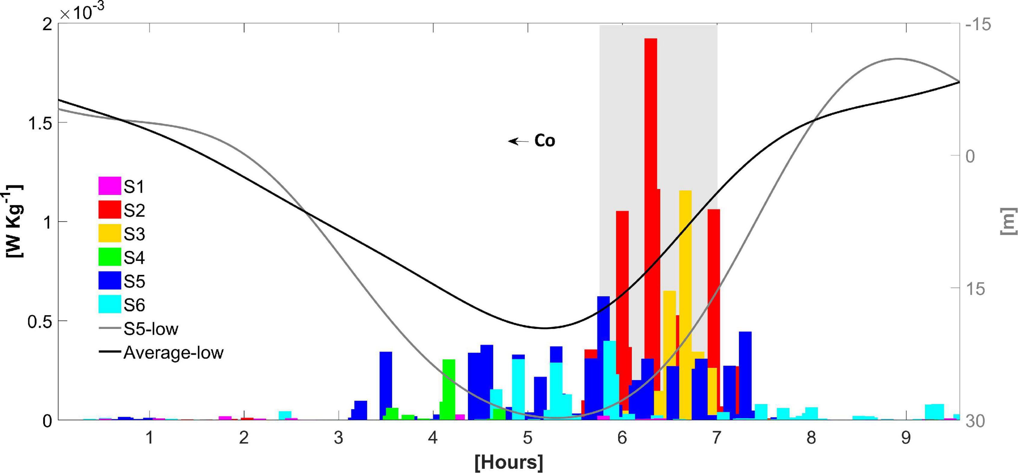
Figure 12. The root-mean-square of the rate of turbulent mixing (in W Kg^–1) throughout the water column (left axis) in the course of the long-wave for each relevant 2-day segment (S1 to S6) on PIL200. The long-wave displacement (in meters, right axis) was computed as the difference between the depth of the undisturbed 20°C isotherm and the depth of this same isotherm low-pass filtered of 3 h, for the wave described in S5 (gray line) and the average for all sections (black line).

In S2, the ebb tides that generated the internal tides were less energetic in comparison to S3, from 0.6 to 0.4 m (Figure 4C, blue line), at the time δ just slightly decreased (Figure 4C, solid black line). Although the environmental conditions were similar, the number of turbulent boluses was augmented in S2, as well as their displacements, with the leading bolus moving the 20°C isotherm ∼ 50 m upward (Figure 6E, T11). Conformingly, the root-mean-square of the rate of turbulent mixing throughout the water column at the rear of the long-wave was the maximum for the period (Figure 12, S2). In the vicinity of this leading jump, the rate of turbulent mixing exceeded 10^–2 W Kg^–1 for the first time (Figure 10E, T11). A number of complicating factors may conspire to explain the intensification of the boluses observed in S2, for instance variations in density offshore or even internal wave-wave interactions (Garrett and Munk, 1979), but a complete review of them is beyond the scope of this work.

Laboratory and numerical experiments of Helfrich (1992) described features similar to S2 following the breaking of an ISW of depression (Helfrich, 1992; see his Figure 2C), such as the presence of a separation in the back of the packet of turbulent boluses (this work, Figure 6E, T12; more clearly seen in Figure 5A, blue arrow) and the formation of cores of mixed fluid within the largest and most intense boluses (Figure 11E, T12 ↔ T13). In fact, the possible formation of a packet of turbulent boluses with trapped cores would make these waves prime candidates for transporting water and material onshore (Lamb, 2002; Klymak and Moum, 2003).

The downslope currents filled almost the length of the long-wave in the lower layers of S3 (Figure 8D) and S2 (Figure 8E). At the position of the turbulent boluses, i.e., the region of breaking, it became overlapped by a prominent intrusion of strong upslope currents in both S3 (Figure 8D, T9 ↔ T10) and S2 (Figure 8E, T12 ↔ T13), with magnitudes up to 0.31 m s^–1 for the latter. A similar pattern of circulation was reported by a breaking ISW of depression simulated by Vlasenko and Hutter (2002; their Figure 7B). These authors concluded that kinematic instabilities explained the mechanism of wave breaking rather than shearing instabilities, even though the zone with Ri < 0.25 occupied an extended area in the region of breaking (Figure 9D, T9 ↔ T10; Figure 9E, T12 ↔ T13). For the two segments, the turbulent boluses elevated the rate of turbulent mixing (Figure 10D, T9 ↔ T10; Figure 10E, T12 ↔ T13) to an extent that significantly eroded the stratification at the upper bound of the interior mixed layer (Figure 11D, T9 ↔ T10; Figure 11E, T12 ↔ T13), producing a new stable vertical fluid stratification (Figure 3A, S3 and S2). This is consistent with laboratory and numerical experiments (e.g., Helfrich, 1992; Bourgault et al., 2014), where the energy of the turbulent boluses was converted into diapycnal mixing as they run-up the slope, bringing colder waters to the surface.

Generally, the first few boluses that emerge are the largest and most intense ones; with time their energy decays and they eventually get overtaken and absorbed during the scattering of additional more energetic ones (Helfrich, 1992). Hence, it is reasonable to suggest that the merged aspect of the packet of boluses in S1 (Figure 6F, T14 ↔ T15) implies a further escalation of the shoaling process in comparison to S2 (S3) at the time the ebb tide increased from 0.4 m (0.6 m) to 1.1 m (Figure 4C, blue line) and δ was slightly closer to the unity (Figure 4C, solid black line). It should also be noted that in this segment, the stratification at the upper bound of the interior mixed layer was the minimum for the period (Figure 11F), implying that an important part of the boluses energy (Figure 10F; also see Figure 9F for reference of the shearing instabilities) had already been converted into mixture. In S1, upslope currents were found to occur within the packet of boluses reaching magnitudes of 0.36 m s^–1, which were the maximum for the period (Figure 8F, T14 ↔ T15).

Bourgault et al. (2007) verified that the local phase speed diminishes accordingly to the shoaling stage of the wave, which implied in speeds as much as two times smaller than the linear phase speed at the time of the turbulent boluses. Therefore, it seems likely that this same process explains the great differences on the phase of the barotropic tides by the time of the arrival of the internal tides. Before wave breaking, the flood tides peaked approximately near the center of the long-waves (Figure 5B, S4 and S5). Whereas after wave breaking the maximum flood were approximately in phase with the rear shoulder of the long-waves and the turbulent boluses existed when the ebb flow slacked and turned onshore (Figure 5A, S2 and S3).

In the literature, turbulent boluses are also commonly referred to as ‘soliton-like waves of elevation’ and/or ‘solitary-like waves with trapped cores’ (Hosegood and van Haren, 2004). These nomenclatures evoke the similarities that exist between the spectrums of the boluses with ISWs. In S3, the wave breaking was likely ongoing and just a small amount of energy scattered into turbulent boluses, reason by which the PSD of displacement did not peak near N_l (Figure 7D). Energy within this spectral band appeared as a narrow peak in S2, when both number and height of the boluses were higher (Figure 7E). In S1, despite the merged aspect of the packet of boluses, the peak about N_l was preserved (Figure 7F). These differ from the PSDs of S6 and S5 as the peak was depicted throughout a broader band of the spectrum and the fall-off rate was less pronounced after N_l (σ⁻³; Figures 7E,F).

Resuspension and Transport

The glider profiles provided a cross shelf view of the hydrodynamic processes derived from the kinematics described in Section “Pre-breaking Waves” and Section “Post-breaking Waves.” At the upper slope, in the vicinity of the 200 m isobath, a region with predominantly upward directed currents was developed in the lower layer, as indicated by the positive values of W_gld (Figure 13C, H1 →). It has been supported by theory (e.g., Vlasenko and Hutter, 2002; Aghsaee et al., 2010; Bourgault et al., 2014) that upward directed currents are produced by turbulent eddies induced by shoaling mode-one waves of depression. Hence, in accordance with the root-mean-square of the rate of turbulent mixing throughout the water column at the NWS edge (Figure 13E, H1 →), which had a maximum value of the order of 10^–4 W Kg^–1. This is the same order of magnitude of the maximum values obtained in S4, S5 and S6 (Figure 12).

FIGURE 13

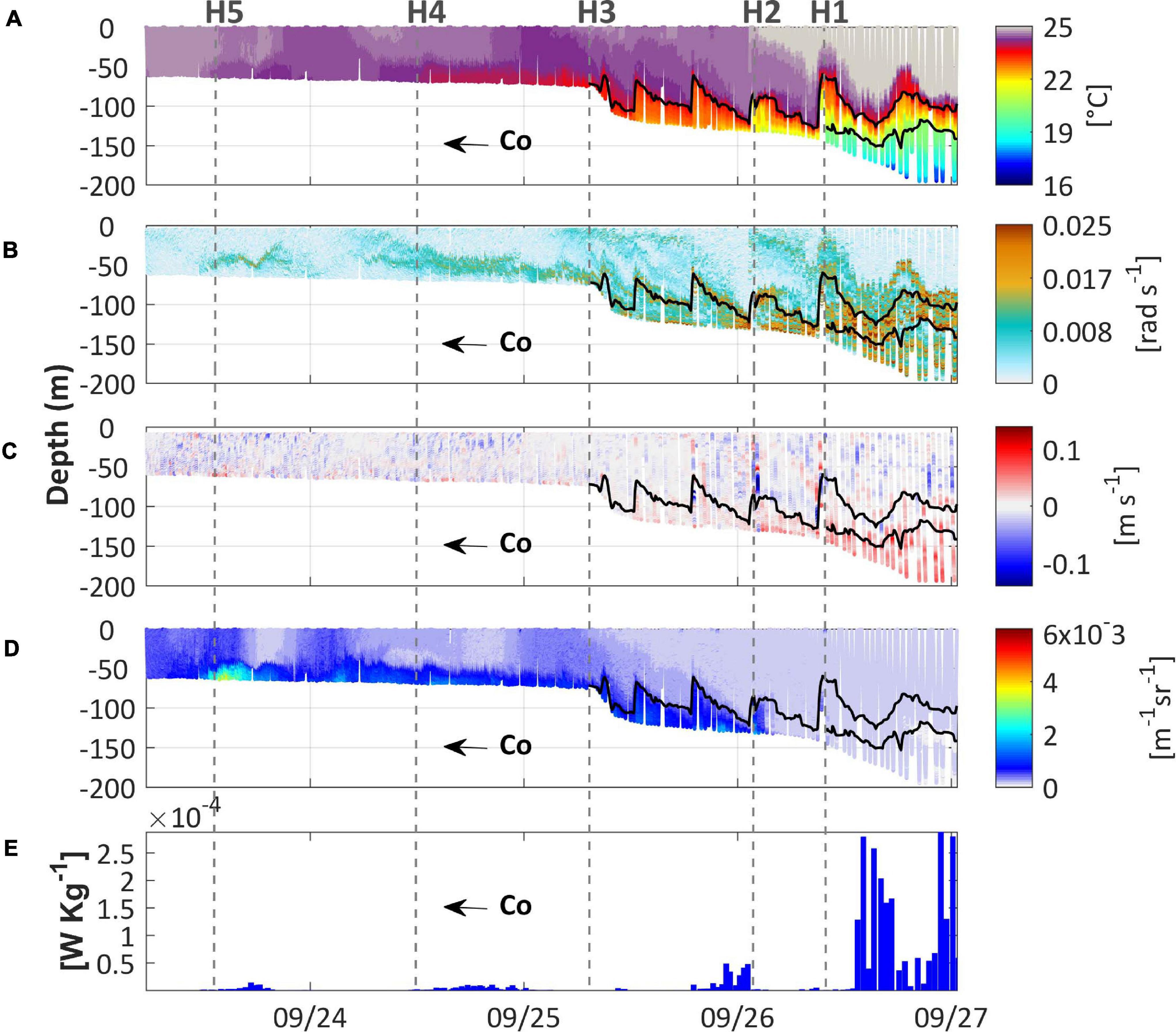
Figure 13. Ocean glider cross-section profiles obtained on September 2013: (A) temperature; (B) Brunt-Väisälä frequency; (C) vertical water velocity calculated from downcast profiles; (D) volumetric backscatter coefficient (VBSC); and (E) the root-mean-square of the rate of turbulent mixing (in W Kg^–1) throughout the water column. In (A–E) c_o indicates the shoreward wave propagation direction. The gray vertical dashed lines identify features referred to in the text. The 20 and 23°C isotherms are displayed on each panel (black solid lines).

Shoaling internal waves and associated turbulent processes have been shown to move sediment upward and maintain bottom nepheloid layers (e.g., Lee et al., 2009; Cheriton et al., 2014; Masunaga et al., 2015). Additionally, the generation of multiple turbulent boluses of trapped cores in the region of breaking, which occurrence was suggested in S2 (Figure 11E, T12 ↔ T13), has not only been addressed an important mechanism to induce resuspension, but also as to transport suspended sediment upslope within the mixed fluid (Bourgault et al., 2014). The repetition of these two processes with semidiurnal periodicity is proposed as a mechanism that produced a zone depleted of suspended material at the upper slope, expressed by means of the minimum values of VBSC (Figure 13D, H1 →). This is in general agreement with the idea that the zone of maximum erosion exists at the breaking site (e.g., Helfrich, 1992; Cacchione et al., 2002; McPhee-Shaw et al., 2004; Bourgault et al., 2014; Cheriton et al., 2014).

Past the thermocline-slope intersection, the genesis of new turbulent boluses is likely interrupted and the wave packet forced by inertia to propagate upslope as an upstream pulsating jet (Helfrich, 1992; Hosegood and van Haren, 2004; Davis and Monismith, 2011). In such cases, the propagating jet behaves as a density current penetrating beneath the lighter water higher on the upper slope. In a manner analogous to the horizontal density intrusion observed onshore of the 150 m isobath (Figure 13A, H2 ↔ H1), where the 20°C isotherm intersected the upper slope. The continuity of the upstream entrainment apparently transported dense waters up onto the shelf, promoting an intensive cooling of the upper layer everywhere onshore of this intersection (Figure 13A, ← H1). Meanwhile, the upstream jet promoted progressively warmer fronts (Figure 13A, H1, H2, H3, H4 and H5), which may explain the lack of a clear pattern of predominant upward directed currents in this region (Figure 13C, ← H1). By the same time the horizontal distribution of VBSC signalized the development of a bottom nepheloid layer that extended continuously for ∼55 km until the maximum intensity of VBSC was reached (Figure 13D, H5 ↔ H2). Besides, the rate of turbulent mixing was weaker compared to the NWS edge, with maximum values of the order of 10^–5 W Kg^–1 in the middle of the upper slope (Figure 13E, nearby H2) and 10^–6 W Kg^–1 on the shelf proper (Figure 13E, ← H3).

The glider profiles obtained during February 2014 depicted a strong stratification throughout the length of the NWS, with a peak in buoyancy at ∼50 m and mixed waters above and below (Figure 14B). This shallower thermocline is an important factor in determining the kinematic nature of the interaction between the internal tides and the topography, since α is very sensitive to variations in stratification. It was found by Holloway et al. (1997) that over the austral summer period only environments internal to the NWS break experienced values of α similar to the ones observed on PIL200. As a consequence, they did not observe strong overturning or mixing events over the upper slope and energy was shown mainly in packets of ISWs. Onshore of the shelf break, the authors described the formation of dispersive packets with waves of elevation (see their Figure 3), which produced thermoclinic displacements strikingly similar to the glider observations taken on February 2014 (Figure 14A, ← H7). Such features induced patches of positive W_gld in the lower layer even onshore from the NWS break (Figure 14C, ← H7), indicating that the source of mixing energy to this layer was more related to turbulent eddies formed during the scattering of ISWs of elevation than to a pulsating jet.

FIGURE 14

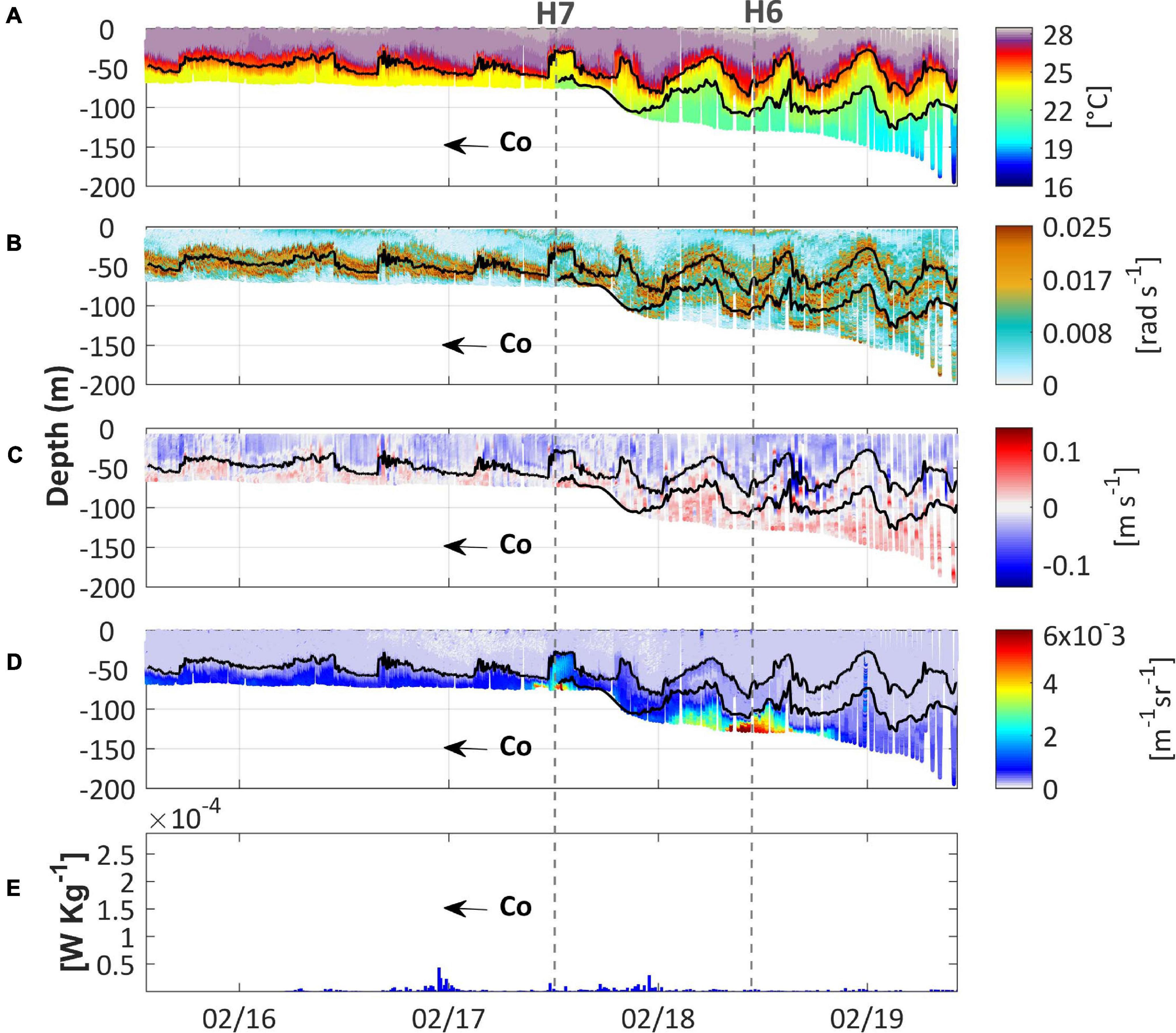
Figure 14. As in Figure 13, but (A–E) for February 2014. The 22 and 25°C isotherms are displayed on each panel (black solid lines). The color bar of the temperature field differs from that of Figure 13.

The processes that governed the kinematics in February 2014 were not sufficiently energetic to erode the stratification (Figure 14B). The maximum values of turbulent mixing were of the order of 10^–6 W Kg^–1 at the NWS edge (Figure 14E, H6 →), increasing to 10^–5 W Kg^–1 along the upper slope and shelf (Figure 14E, ← H6). Meanwhile, the temperature field was nearly homogeneous along the cross-shelf transect of the glider (Figure 14A), with the exception of an upstream jet of cold waters (Figure 14A, H7). This feature was observed after the intersection of the 22°C isotherm with the shelf break, extending for ∼4 km onshore. Moreover, the glider profiles revealed that the development of a bottom nepheloid layer was ubiquitous for the period (Figure 14D), without the presence of a zone depleted of suspended material at the upper slope or anywhere else. Recent work carried out on the NWS (Zulberti et al., 2020) has revealed that the passage of a packet of waves of depression may indeed maintain a near-bed layer of suspended sediment, even when there is no evidence of wave breaking.

Dufois et al. (2017) have shown that the suspended material across the NWS is primarily composed of muds, which are most likely transported downslope (McLoughlin and Young, 1985; Belde et al., 2017) given that this region is ebb-dominated (Holloway, 1983b; Porter-Smith et al., 2004). On the assumption that the VBSC during the glider mission of February 2014 was most intense at the upper slope (Figure 14D, H6) in response to the local barotropic tide, the baroclinic counterpart of the tide is ascribed as the potential conduit for muds from the upper slope to the shelf. For example, surging within an upstream jet of cold waters (Figure 14D, H7). Such upstream entrainment of muds was much stronger during the glider mission of September 2013 (Figure 13D, H5). Since the rate of turbulent mixing in the vicinity of the 200 m isobath was two orders of magnitude greater during this mission, it seems likely that the shoaling and breaking of internal tides in the region played a critical role in this difference.

Conclusion

Although the knowledge of nonlinear internal tide dynamics on the Australian NWS is well established during the austral summer, comparatively little is known about the consequences of the setup of a near-bottom thermocline under austral wintertime conditions. In this paper, we examined field observations of semidiurnal internal tides as they shoal, break and run-up as turbulent boluses across the edge of the NWS, offshore Dampier, during September 2013. To the best of our knowledge, this is the first conclusive field evidence of internal wave breaking observed in this region.

On first consideration, the evidence of wave breaking is based on the internal waveforms and wavefields measured through an oceanographic mooring on the upper slope (PIL200). In essence, frontal tidal bores previously observed by field studies over the summer periods in this region gave way to rear face bores. Several laboratory and numerical papers have described this behavior of wave shoaling preceding wave breaking. When the incident wave encountered environments of relatively weak nonlinear steepening, dispersive effects went harsh enough to spread energy out of the semidiurnal wave to a dispersive wave packet of short-period ISWs. On the other hand, when dispersion was considered small compared to the cumulative effect of nonlinear steepening, the semidiurnal wave built sufficient energy at its rear face to produce wave breaking and, as a consequence, a large amount of energy was scattered into packets of turbulent boluses. The rate of turbulent mixing associated to these features was the maximum for the period, sometimes exceeding 10^–2 W Kg^–1. This value is seven orders of magnitude greater than that observed in a typical open ocean (Lien et al., 2012).

Measurements obtained through autonomous ocean glider profiles revealed the shelf-wide hydrodynamic consequences of the kinematics described on PIL200. The results indicated that the shoaling and breaking of internal tides, and the consecutive run-up of turbulent boluses, led to the overmixing of water layers, remarkably onshore from the thermocline-slope intersection. Incipient benthic processes associated with these processes apparently eroded material over the upper slope and the run-up of turbulent boluses, which sometimes was forced by inertia to propagate as an upstream pulsating jet, were described as the potential conduits for the onshore transport of cold waters and suspended materials. This represents a fundamental broadening of our understanding of how the muds of the upper slope are transferred to the ebb-dominated NWS.

Data Availability Statement

The datasets analyzed for this study can be found in the Australian Ocean Data Network (https://portal.aodn.org.au).

Author Contributions

GL and CP designed the study. GL performed the data analysis and processing under supervision from CL and CP. GL wrote the manuscript with the help and inputs from all co-authors. All authors contributed to the article and approved the submitted version.

Funding

This study was financed in part by the Coordenação de Aperfeiçoamento de Pessoal de Nível Superior-Brasil (CAPES). The first author was supported by a scholarship provided by the National Council for Scientific and Technological Development (CNPQ; Grant No. 133201/2017-1). The third author also would like to thank CNPQ for the research fellowship (CNPQ, process 380671/2020-4) and for the research project (Grant No. 429454/2016-3) which part of this work was conducted. The ocean glider and oceanographic mooring data used in this paper were sourced from Australia’s Integrated Marine Observing System (IMOS) – IMOS is enabled by the National Collaborative Research Infrastructure Strategy (NCRIS). It is operated by a consortium of institutions as an unincorporated joint venture, with the University of Tasmania as Lead Agent. The mooring data used in this paper were collected by the Australian Institute of Marine Science (AIMS), a sub-facility of the Australian National Mooring Network (ANMN). The ocean glider data were collected by the IMOS Ocean Glider facility located at the University of Western Australia.

Conflict of Interest

The authors declare that the research was conducted in the absence of any commercial or financial relationships that could be construed as a potential conflict of interest.

Supplementary Material

The Supplementary Material for this article can be found online at: https://www.frontiersin.org/articles/10.3389/fmars.2021.629372/full#supplementary-material

References

Aghsaee, P., Boegman, L., and Lamb, K. G. (2010). Breaking of shoaling internal solitary waves. J. Fluid Mech. 659, 289–317. doi: 10.1017/S002211201000248X

CrossRef Full Text | Google Scholar

Bahmanpour, M. H., Pattiaratchi, C., Wijeratne, E. S., Steinberg, C., and D’Adamo, N. (2016). Multi-year observation of Holloway current along the shelf edge of north western Australia. J. Coast. Res. 75, 517–521. doi: 10.2112/SI75-104.1

CrossRef Full Text | Google Scholar

Baines, P. G. (1981). Satellite observations of internal waves on the Australian north-west shelf. Mar. Freshw. Res. 32, 457–463. doi: 10.1071/MF9810457

CrossRef Full Text | Google Scholar

Belde, J., Reuning, L., and Back, S. (2017). Bottom currents and sediment waves on a shallow carbonate shelf, Northern Carnarvon Basin, Australia. Cont. Shelf Res. 138, 142–153. doi: 10.1016/j.csr.2017.03.007

CrossRef Full Text | Google Scholar

Boczar-Karakiewicz, B., Bona, J. L., and Pelchat, B. (1991). Interaction of internal waves with the seabed on continental shelves. Cont. Shelf Res. 11, 1181–1197. doi: 10.1016/0278-4343(91)90096-O

CrossRef Full Text | Google Scholar

Boegman, L., Imberger, J., Ivey, G. N., and Antenucci, J. P. (2003). High−frequency internal waves in large stratified lakes. Limnol. Oceanogr. 48, 895–919. doi: 10.4319/lo.2003.48.2.0895

CrossRef Full Text | Google Scholar

Boegman, L., Ivey, G. N., and Imberger, J. (2005). The degeneration of internal waves in lakes with sloping topography. Limnol. Oceanogr. 50, 1620–1637. doi: 10.4319/lo.2005.50.5.1620

CrossRef Full Text | Google Scholar

Boehm, A. B., Sanders, B. F., and Winant, C. D. (2002). Cross-shelf transport at Huntington Beach. Implications for the fate of sewage discharged through an offshore ocean outfall. Environ. Sci. Technol. 36, 1899–1906. doi: 10.1021/es0111986

PubMed Abstract | CrossRef Full Text | Google Scholar

Bogucki, D., Dickey, T., and Redekopp, L. G. (1997). Sediment resuspension and mixing by resonantly generated internal solitary waves. J. Phys. Oceanogr. 27, 1181–1196. doi: 10.1175/1520-04851997027<1181:SRAMBR<2.0.CO;2

CrossRef Full Text | Google Scholar

Bourgault, D., Blokhina, M. D., Mirshak, R., and Kelley, D. E. (2007). Evolution of a shoaling internal solitary wavetrain. Geophys. Res. Lett. 34:L03601. doi: 10.1029/2006GL028462

CrossRef Full Text | Google Scholar

Bourgault, D., Morsilli, M., Richards, C., Neumeier, U., and Kelley, D. E. (2014). Sediment resuspension and nepheloid layers induced by long internal solitary waves shoaling orthogonally on uniform slopes. Cont. Shelf Res. 72, 21–33. doi: 10.1016/j.csr.2013.10.019

CrossRef Full Text | Google Scholar

Cacchione, D. A., and Southard, J. B. (1974). Incipient sediment movement by shoaling internal gravity waves. J. Geophys. Res. 79, 2237–2242. doi: 10.1029/JC079i015p02237

CrossRef Full Text | Google Scholar

Cacchione, D. A., Pratson, L. F., and Ogston, A. S. (2002). The shaping of continental slopes by internal tides. Science 296, 724–727. doi: 10.1126/science.1069803

PubMed Abstract | CrossRef Full Text | Google Scholar

Cai, S., Long, X., Dong, D., and Wang, S. (2008). Background current affects the internal wave structure of the northern South China Sea. Prog. Nat. Sci. 18, 585–589. doi: 10.1016/j.pnsc.2007.11.019

CrossRef Full Text | Google Scholar

Carter, G. S., Gregg, M. C., and Lien, R. C. (2005). Internal waves, solitary-like waves, and mixing on the Monterey Bay shelf. Cont. Shelf Res. 25, 1499–1520. doi: 10.1016/j.csr.2005.04.011

CrossRef Full Text | Google Scholar

Chen, G. Y., Wu, R. J., and Wang, Y. H. (2010). Interaction between internal solitary waves and an isolated atoll in the Northern South China Sea. Ocean Dyn. 60, 1285–1292. doi: 10.1007/s10236-010-0323-1

CrossRef Full Text | Google Scholar

Chen, W. (2011). Status and challenges of Chinese deepwater oil and gas development. Pet. Sci. 8, 477–484. doi: 10.1007/s12182-011-0171-8

CrossRef Full Text | Google Scholar

Cheriton, O. M., McPhee-Shaw, E. E., Shaw, W. J., Stanton, T. P., Bellingham, J. G., and Storlazzi, C. D. (2014). Suspended particulate layers and internal waves over the southern Monterey Bay continental shelf: an important control on shelf mud belts? J. Geophys. Res. 119, 428–444. doi: 10.1002/2013JC009360

CrossRef Full Text | Google Scholar

Colosi, J. A., Beardsley, R. C., Lynch, J. F., Gawarkiewicz, G., Chiu, C. S., and Scotti, A. (2001). Observations of nonlinear internal waves on the outer New England continental shelf during the summer Shelfbreak Primer study. J. Geophys. Res. 106, 9587–9601. doi: 10.1029/2000JC900124

CrossRef Full Text | Google Scholar

Craig, P. D. (1988). A numerical model study of internal tides on the Australian northwest shelf. J. Mar. Res. 46, 59–76. doi: 10.1357/002224088785113676

CrossRef Full Text | Google Scholar

Davis, K. A., and Monismith, S. G. (2011). The modification of bottom boundary layer turbulence and mixing by internal waves shoaling on a barrier reef. J. Phys. Oceanogr. 41, 2223–2241. doi: 10.1175/2011JPO4344.1

CrossRef Full Text | Google Scholar

Diamessis, P. J., and Redekopp, L. G. (2006). Numerical investigation of solitary internal wave-induced global instability in shallow water benthic boundary layers. J. Phys. Oceanogr. 36, 784–812. doi: 10.1175/JPO2900.1

CrossRef Full Text | Google Scholar

Dillon, T. M. (1982). Vertical overturns: a comparison of Thorpe and Ozmidov length scales. J. Geophys. Res. 87, 9601–9613. doi: 10.1029/JC087iC12p09601

CrossRef Full Text | Google Scholar

Dufois, F., Lowe, R. J., Branson, P., and Fearns, P. (2017). Tropical cyclone−driven sediment dynamics over the Australian north west shelf. J. Geophys. Res. 122, 10225–10244. doi: 10.1002/2017JC013518

CrossRef Full Text | Google Scholar

Dunphy, M., Subich, C., and Stastna, M. (2011). Spectral methods for internal waves: indistinguishable density profiles and double-humped solitary waves. Nonlinear Process. Geophys. 18, 351–358. doi: 10.5194/npg-18-351-2011

CrossRef Full Text | Google Scholar

Freeman, W. J., and Zhai, J. (2009). Simulated power spectral density (PSD) of background electrocorticogram (ECoG). Cogn. Neurodyn. 3, 97–103. doi: 10.1007/s11571-008-9064-y

PubMed Abstract | CrossRef Full Text | Google Scholar

Garrett, C., and Munk, W. (1979). Internal waves in the ocean. Annu Rev. Fluid Mech. 11, 339–369.

Google Scholar

Gerkema, T., and Zimmerman, J. T. F. (2008). An Introduction to Internal Waves. Lecture Notes. Texel: Royal NIOZ.

Google Scholar

Gregg, M., Sanford, T., and Winkel, D. (2003). Reduced mixing from the breaking of internal waves in equatorial waters. Nature 422, 513–515. doi: 10.1038/nature01507

PubMed Abstract | CrossRef Full Text | Google Scholar

Helfrich, K. R. (1992). Internal solitary wave breaking and run-up on a uniform slope. J. Fluid Mech. 243, 133–154. doi: 10.1017/S0022112092002660

CrossRef Full Text | Google Scholar

Helfrich, K. R., and Melville, W. K. (2006). Long nonlinear internal waves. Annu. Rev. Fluid Mech. 38, 395–425. doi: 10.1146/annurev.fluid.38.050304.092129

CrossRef Full Text | Google Scholar

Helfrich, K., and Melville, W. (1986). On long nonlinear internal waves over slope-shelf topography. J. Fluid Mech. 167, 285–308. doi: 10.1017/S0022112086002823

CrossRef Full Text | Google Scholar

Henyey, F. S., and Hoering, A. (1997). Energetics of borelike internal waves. J. Geophys. Res. 102, 3323–3330. doi: 10.1029/96JC03558

CrossRef Full Text | Google Scholar

Holloway, P. E. (1983a). Internal tides on the Australian north-west shelf: a preliminary investigation. J. Phys. Oceanogr. 13, 1357–1370. doi: 10.1175/1520-04851983013<1357:ITOTAN<2.0.CO;2

CrossRef Full Text | Google Scholar

Holloway, P. E. (1983b). Tides on the Australian north-west shelf. Mar. Freshw. Res. 34, 213–230. doi: 10.1071/MF9830213

CrossRef Full Text | Google Scholar

Holloway, P. E. (1984). On the semidiurnal internal tide at a shelf-break region on the Australian north west shelf. J. Phys. Oceanogr. 14, 1787–1799. doi: 10.1175/1520-04851984014<1787:OTSITA<2.0.CO;2

CrossRef Full Text | Google Scholar

Holloway, P. E. (1987). Internal hydraulic jumps and solitons at a shelf break region on the Australian north west shelf. J. Geophys. Res. 92, 5405–5416. doi: 10.1029/JC092iC05p05405

CrossRef Full Text | Google Scholar

Holloway, P. E. (1994). Observations of internal tide propagation on the Australian north west shelf. J. Phys. Oceanogr. 24, 1706–1716. doi: 10.1175/1520-04851994024<1706:OOITPO<2.0.CO;2

CrossRef Full Text | Google Scholar

Holloway, P. E., Chatwin, P. G., and Craig, P. (2001). Internal tide observations from the Australian north west shelf in summer 1995. J. Phys. Oceanogr. 31, 1182–1199. doi: 10.1175/1520-04852001031<1182:ITOFTA<2.0.CO;2

CrossRef Full Text | Google Scholar

Holloway, P. E., Humphries, S. E., Atkinson, M., and Imberger, J. (1985). Mechanisms for nitrogen supply to the Australian north west shelf. Mar. Freshw. Res. 36, 753–764. doi: 10.1071/MF9850753

CrossRef Full Text | Google Scholar

Holloway, P. E., Pelinovsky, E., Talipova, T., and Barnes, B. (1997). A nonlinear model of internal tide transformation on the Australian north west shelf. J. Phys. Oceanogr. 27, 871–896. doi: 10.1175/1520-04851997027<0871:ANMOIT<2.0.CO;2

CrossRef Full Text | Google Scholar

Holloway, P., Pelinovsky, E., and Talipova, T. (2003). “Internal tide transformation and oceanic internal solitary waves,” in Environmental Stratified Flows. Topics in Environmental Fluid Mechanics, Vol. 3, ed. R. Grimshaw, (Boston, MA: Springer), 29–60. doi: 10.1007/0-306-48024-7_2

CrossRef Full Text | Google Scholar

Hosegood, P., and van Haren, H. (2004). Near-bed solibores over the continental slope in the Faeroe-Shetland Channel. Deep Sea Res. II Top. Stud. Oceanogr. 51, 2943–2971. doi: 10.1016/j.dsr2.2004.09.016

CrossRef Full Text | Google Scholar

Hosegood, P., and van Haren, H. (2006). Sub-inertial modulation of semi-diurnal currents over the continental slope in the Faeroe-Shetland Channel. Deep Sea Res. I Oceanogr. Res. Pap. 53, 627–655. doi: 10.1016/j.dsr.2005.12.016

CrossRef Full Text | Google Scholar

Huthnance, J. M. (1989). Internal tides and waves near the continental shelf edge. Geophys. Astrophys. Fluid Dyn. 48, 81–106. doi: 10.1080/03091928908219527

CrossRef Full Text | Google Scholar

Johnson, D. R., Weidemann, A., and Pegau, W. S. (2001). Internal tidal bores and bottom nepheloid layers. Cont. Shelf Res. 21, 1473–1484. doi: 10.1016/S0278-4343(00)00109-6

CrossRef Full Text | Google Scholar

Jones, H. A. (1970). The sediments, structure, and morphology of the northwest Australian continental shelf between Rowley Shoals and Monte Bello Islands. Record 1970/027. Geoscience Australia, Canberra. Avalaible online at: http://pid.geoscience.gov.au/dataset/ga/12440

Google Scholar

Jones, N. L., and Ivey, G. N. (2017). “Internal waves,” in Encyclopedia of Maritime and Offshore Engineering, eds J. Carlton, P. Jukes, and Y. S. Choo, (Hoboken, NJ: John Wiley & Sons). doi: 10.1002/9781118476406.emoe089

CrossRef Full Text | Google Scholar

Jones, N. L., Ivey, G. N., Rayson, M. D., and Kelly, S. M. (2020). Mixing driven by breaking nonlinear internal waves. Geophys. Res. Lett. 47:e2020GL089591. doi: 10.1029/2020GL089591

CrossRef Full Text | Google Scholar

Klink, J. (1999). Dynmodes: Matlab code for Normal Modes Analysis. Woods Hole (MA): Woods Hole Science Center, SEA-MAT, Matlab tools for oceanographic analysis. Available online at: http://woodshole.er.usgs.gov/operations/sea-mat/index.html

Google Scholar

Klymak, J. M., and Moum, J. N. (2003). Internal solitary waves of elevation advancing on a shoaling shelf. Geophys. Res. Lett. 30:2045. doi: 10.1029/2003GL017706

CrossRef Full Text | Google Scholar

Lamb, K. G. (1994). Numerical experiments of internal wave generation by strong tidal flow across a finite amplitude bank edge. J. Geophys. Res. 99, 843–864. doi: 10.1029/93JC02514

CrossRef Full Text | Google Scholar

Lamb, K. G. (2002). A numerical investigation of solitary internal waves with trapped cores formed via shoaling. J. Fluid Mech. 451, 109–144. doi: 10.1017/S002211200100636X

CrossRef Full Text | Google Scholar

Lamb, K. G., and Nguyen, V. T. (2009). Calculating energy flux in internal solitary waves with an application to reflectance. J. Phys. Oceanogr. 39, 559–580. doi: 10.1175/2008JPO3882.1

CrossRef Full Text | Google Scholar

Lamb, K. G., and Warn-Varnas, A. (2015). Two-dimensional numerical simulations of shoaling internal solitary waves at the ASIAEX site in the South China Sea. Nonlinear Process. Geophys. 22, 289–312. doi: 10.5194/npg-22-289-2015

CrossRef Full Text | Google Scholar

Lansing, F. S., and Maxworthy, T. (1984). On the generation and evolution of internal gravity waves. J. Fluid Mech. 145, 127–149. doi: 10.1017/S0022112084002846

CrossRef Full Text | Google Scholar

Lee, I. H., Lien, R. C., Liu, J. T., and Chuang, W. S. (2009). Turbulent mixing and internal tides in Gaoping (Kaoping) submarine canyon, Taiwan. J. Mar. Syst. 76, 383–396. doi: 10.1016/j.jmarsys.2007.08.005

CrossRef Full Text | Google Scholar

Leichter, J. J., Wing, S. R., Miller, S. L., and Denny, M. W. (1996). Pulsed delivery of subthermocline water to Conch Reef (Florida Keys) by internal tidal bores. Limnol. Oceanogr. 41, 1490–1501. doi: 10.4319/lo.1996.41.7.1490

CrossRef Full Text | Google Scholar

Liao, G., Yuan, Y., Arata, K., Yang, C., Chen, H., Naokazu, T., et al. (2011). Analysis of internal tidal characteristics in the layer above 450 m from acoustic Doppler current profiler observations in the Luzon Strait. Sci. China Earth Sci. 54, 1078–1094. doi: 10.1007/s11430-010-4102-0

CrossRef Full Text | Google Scholar

Lien, R. C., D’Asaro, E. A., Henyey, F., Chang, M. H., Tang, T. Y., and Yang, Y. J. (2012). Trapped core formation within a shoaling nonlinear internal wave. J. Phys. Oceanogr. 42, 511–525. doi: 10.1175/2011JPO4578.1

CrossRef Full Text | Google Scholar

Lim, K., Ivey, G. N., and Nokes, R. I. (2008). The generation of internal waves by tidal flow over continental shelf/slope topography. Environ. Fluid Mech. 8:511. doi: 10.1007/s10652-008-9085-4

CrossRef Full Text | Google Scholar

Mahjabin, T., Pattiaratchi, C., and Hetzel, Y. (2020). Occurrence and seasonal variability of dense shelf water cascades along Australian continental shelves. Sci. Rep. 10:9732. doi: 10.1038/s41598-020-66711-5

PubMed Abstract | CrossRef Full Text | Google Scholar

Mater, B. D., Venayagamoorthy, S. K., St. Laurent, L., and Moum, J. N. (2015). Biases in Thorpe-scale estimates of turbulence dissipation. Part I: Assessments from large-scale overturns in oceanographic data. J. Phys. Oceanogr., 45, 2497–2521. doi: 10.1175/JPO-D-14-0128.1

CrossRef Full Text | Google Scholar

Masunaga, E., Homma, H., Yamazaki, H., Fringer, O. B., Nagai, T., Kitade, Y., et al. (2015). Mixing and sediment resuspension associated with internal bores in a shallow bay. Cont. Shelf Res. 110, 85–99. doi: 10.1016/j.csr.2015.09.022

CrossRef Full Text | Google Scholar

Maxworthy, T. (1980). On the formation of nonlinear internal waves from the gravitational collapse of mixed regions in two and three dimensions. J. Fluid Mech. 96, 47–64. doi: 10.1017/S0022112080002017

CrossRef Full Text | Google Scholar

McLoughlin, R. J., and Young, P. C. (1985). Sedimentary provinces of the fishing grounds of the north west shelf of Australia: grain-size frequency analysis of surficial sediments. Mar. Freshw. Res. 36, 671–681. doi: 10.1071/MF9850671

CrossRef Full Text | Google Scholar

McPhee-Shaw, E. E., Sternberg, R. W., Mullenbach, B., and Ogston, A. S. (2004). Observations of intermediate nepheloid layers on the northern California continental margin. Cont. Shelf Res. 24, 693–720. doi: 10.1016/j.csr.2004.01.004

CrossRef Full Text | Google Scholar

Merckelbach, L., Smeed, D., and Griffiths, G. (2010). Vertical water velocities from underwater gliders. J. Atmos. Ocean. Technol. 27, 547–563. doi: 10.1175/2009JTECHO710.1

CrossRef Full Text | Google Scholar

Michallet, H., and Ivey, G. N. (1999). Experiments on mixing due to internal solitary waves breaking on uniform slopes. J. Geophys. Res. 104, 13467–13477. doi: 10.1029/1999JC900037

CrossRef Full Text | Google Scholar

Miller, J. A., and Shanks, A. L. (2004). Ocean-estuary coupling in the Oregon upwelling region: abundance and transport of juvenile fish and of crab megalopae. Mar. Ecol. Prog. Ser. 271, 267–279. doi: 10.3354/meps271267

CrossRef Full Text | Google Scholar

Moum, J. N., Farmer, D. M., Smyth, W. D., Armi, L., and Vagle, S. (2003). Structure and generation of turbulence at interfaces strained by internal solitary waves propagating shoreward over the continental shelf. J. Phys. Oceanogr. 33, 2093–2112. doi: 10.1175/1520-04852003033<2093:SAGOTA<2.0.CO;2

CrossRef Full Text | Google Scholar

Nam, S., and Send, U. (2011). Direct evidence of deep water intrusions onto the continental shelf via surging internal tides. J. Geophys. Res. 116:C05004. doi: 10.1029/2010JC006692

CrossRef Full Text | Google Scholar

Noble, M., Jones, B., Hamilton, P., Xu, J., Robertson, G., Rosenfeld, L., et al. (2009). Cross-shelf transport into nearshore waters due to shoaling internal tides in San Pedro Bay, CA. Cont. Shelf Res. 29, 1768–1785. doi: 10.1016/j.csr.2009.04.008

CrossRef Full Text | Google Scholar

Orr, M. H., and Mignerey, P. C. (2003). Nonlinear internal waves in the South China Sea: Observation of the conversion of depression internal waves to elevation internal waves. J. Geophys. Res.: Oceans, 108(C3). doi: 10.1029/2001JC001163

CrossRef Full Text | Google Scholar

Pattiaratchi, C., Woo, L. M., Thomson, P. G., Hong, K. K., and Stanley, D. (2017). Ocean glider observations around Australia. Oceanography 30, 90–91. doi: 10.5670/oceanog.2017.226

CrossRef Full Text | Google Scholar

Petrenko, A. A., Jones, B. H., Dickey, T. D., and Hamilton, P. (2000). Internal tide effects on a sewage plume at Sand Island, Hawaii. Cont. Shelf Res. 20, 1–13. doi: 10.1016/S0278-4343(99)00060-6

CrossRef Full Text | Google Scholar

Pineda, J. (1991). Predictable upwelling and the shoreward transport of planktonic larvae by internal tidal bores. Science 253, 548–549. doi: 10.1126/science.253.5019.548

PubMed Abstract | CrossRef Full Text | Google Scholar

Porter-Smith, R., Harris, P. T., Andersen, O. B., Coleman, R., Greenslade, D., and Jenkins, C. J. (2004). Classification of the Australian continental shelf based on predicted sediment threshold exceedance from tidal currents and swell waves. Mar. Geol. 211, 1–20. doi: 10.1016/j.margeo.2004.05.031

CrossRef Full Text | Google Scholar

Quaresma, L. S., Vitorino, J., Oliveira, A., and da Silva, J. (2007). Evidence of sediment resuspension by nonlinear internal waves on the western Portuguese mid-shelf. Mar. Geol. 246, 123–143. doi: 10.1016/j.margeo.2007.04.019

CrossRef Full Text | Google Scholar

Rayson, M. D., Jones, N. L., and Ivey, G. N. (2019). Observations of large-amplitude mode-2 nonlinear internal waves on the Australian north west shelf. J. Phys. Oceanogr. 49, 309–328. doi: 10.1175/JPO-D-18-0097.1

CrossRef Full Text | Google Scholar

Saffarinia, K., and Kao, T. W. (1996). Numerical study of the breaking of an internal soliton and its interaction with a slope. Dyn. Atmos. Oceans 23, 379–391. doi: 10.1016/0377-0265(95)00428-9

CrossRef Full Text | Google Scholar

Sandstrom, H., and Elliott, J. A. (1984). Internal tide and solitons on the Scotian shelf: a nutrient pump at work. J. Geophys. Res. 89, 6415–6426. doi: 10.1029/JC089iC04p06415

CrossRef Full Text | Google Scholar

Shearman, R. K., and Brink, K. H. (2010). Evaporative dense water formation and cross-shelf exchange over the northwest Australian inner shelf. J. Geophys. Res. 115:C06027. doi: 10.1029/2009JC005931

CrossRef Full Text | Google Scholar

Shi, X. G., Fan, Z. S., and Liu, H. L. (2009). A numerical calculation method for eigenvalue problems of nonlinear internal waves. J. Hydrodyn. Ser. B 21, 373–378. doi: 10.1016/S1001-6058(08)60159-6

CrossRef Full Text | Google Scholar

Small, J., Sawyer, T. C., and Scott, J. C. (1999). The evolution of an internal bore at the Malin shelf break. Ann. Geophys. 17, 547–565. doi: 10.1007/s00585-999-0547-x

CrossRef Full Text | Google Scholar

Smyth, N. F., and Holloway, P. E. (1988). Hydraulic jump and undular bore formation on a shelf break. J. Phys. Oceanogr. 18, 947–962. doi: 10.1175/1520-04851988018<0947:HJAUBF<2.0.CO;2

CrossRef Full Text | Google Scholar

Stastna, M., and Lamb, K. G. (2002). Large fully nonlinear internal solitary waves: the effect of background current. Phys. Fluids 14, 2987–2999. doi: 10.1063/1.1496510

CrossRef Full Text | Google Scholar

Sutherland, B. R., and Nault, J. T. (2007). Intrusive gravity currents propagating along thin and thick interfaces. J. Fluid Mech. 586, 109–118. doi: 10.1017/S0022112007007288

CrossRef Full Text | Google Scholar

Sutherland, B. R., Barrett, K. J., and Ivey, G. N. (2013). Shoaling internal solitary waves. J. Geophys. Res. 118, 4111–4124. doi: 10.1002/jgrc.20291

CrossRef Full Text | Google Scholar

Thorpe, S. A. (1977). Turbulence and mixing in a Scottish loch. Philos. Trans. R. Soc. London Ser. A Math. Phys. Sci. 286, 125–181. doi: 10.1098/rsta.1977.0112

CrossRef Full Text | Google Scholar

Van Gastel, P., Ivey, G. N., Meuleners, M. J., Antenucci, J. P., and Fringer, O. (2009). The variability of the large-amplitude internal wave field on the Australian north west shelf. Cont. Shelf Res. 29, 1373–1383. doi: 10.1016/j.csr.2009.02.006

CrossRef Full Text | Google Scholar

Vlasenko, V., and Hutter, K. (2002). Numerical experiments on the breaking of solitary internalwaves over a slope-shelf topography. J. Phys. Oceanogr. 32, 1779–1793. doi: 10.1175/1520-04852002032<1779:NEOTBO<2.0.CO;2

CrossRef Full Text | Google Scholar

Vlasenko, V., Stashchuk, N., and Hutter, K. (2005). Baroclinic Tides: Theoretical Modeling and Observational Evidence. Cambridge: Cambridge University Press.

Google Scholar

Vlasenko, V., and Stashchuk, N. (2007). Three-dimensional shoaling of large-amplitude internal waves. J. Geophys. Res.: Oceans, 112(C11). doi: 10.1029/2007JC004107

CrossRef Full Text | Google Scholar

Walter, R. K., Stastna, M., Woodson, C. B., and Monismith, S. G. (2016). Observations of nonlinear internal waves at a persistent coastal upwelling front. Cont. Shelf Res. 117, 100–117. doi: 10.1016/j.csr.2016.02.007

CrossRef Full Text | Google Scholar

Wesson, J. C., and Gregg, M. C. (1994). Mixing at Camarinal sill in the Strait of Gibraltar. J. Geophys. Res. 99, 9847–9878. doi: 10.1029/94JC00256

CrossRef Full Text | Google Scholar

Wijeratne, S., Pattiaratchi, C., and Proctor, R. (2018). Estimates of surface and subsurface boundary current transport around Australia. J. Geophys. Res. 123, 3444–3466. doi: 10.1029/2017JC013221

CrossRef Full Text | Google Scholar

Wijesekera, H. W., and Dillon, T. M. (1991). Internal waves and mixing in the upper equatorial Pacific Ocean. J. Geophys. Res. 96, 7115–7125. doi: 10.1029/90JC02727

CrossRef Full Text | Google Scholar

Woo, M. (2017). Australian National Facility for Ocean Gliders (ANFOG) Data Management User Manual. Available online at: https://imos.org.au/fileadmin/user_upload/shared/ANFOG/ANFOG_DataManagement_UsersManual_v5_Nov28.pdf

Google Scholar

Xie, X. H., Cuypers, Y., Bouruet-Aubertot, P., Pichon, A., Lourenço, A., and Ferron, B. (2015). Generation and propagation of internal tides and solitary waves at the shelf edge of the Bay of Biscay. J. Geophys. Res. 120, 6603–6621. doi: 10.1002/2015JC010827

CrossRef Full Text | Google Scholar

Xu, Z., Yin, B., and Hou, Y. (2010). Highly nonlinear internal solitary waves over the continental shelf of the northwestern South China Sea. Chin. J. Oceanol. Limnol. 28, 1049–1054. doi: 10.1007/s00343-010-9018-1

CrossRef Full Text | Google Scholar

Zulberti, A., Jones, N. L., and Ivey, G. N. (2020). Observations of enhanced sediment transport by non−linear internal waves. Geophys. Res. Lett. 47:e2020GL088499. doi: 10.1029/2020GL088499

CrossRef Full Text | Google Scholar