 Johanna Medellín-Mora
 Rubén Escribano1
 Andrea Corredor-Acosta
 Wolfgang Schneider
- 1Instituto Milenio de Oceanografía and Departamento de Oceanografía, Facultad de Ciencias Naturales y Oceanográficas, Universidad de Concepción, Concepción, Chile
- 2Departamento de Física, Facultad de Ciencias, Universidad del Bío-Bío, Concepción, Chile
The subtropical gyres occupy approximately 40% of the surface of the Earth and are widely recognized as oligotrophic zones. Among them, the South Pacific subtropical gyre (SPSG) shows the lowest chlorophyll-a levels (0.02–0.04 μgL–1), the deepest nutricline (>200 m) and euphotic zone (∼160 m), and the lowest rates of nitrogen fixation. The zooplankton community is poorly known in the SPSG. We report a study focused on the composition and distribution of pelagic copepods within the gyre so as to uncover the diversity and habitat conditions of this special community. Therefore, during the austral spring of 2015, an oceanographic cruise was conducted across the eastern side of the SPSG. Physical and chemical variables were measured in the upper 1000 m, while zooplankton samples were collected by means of vertically stratified hauls using a multiple net sampler for five layers (0–800 m). Satellite data were also used to assess near-surface phytoplankton biomass (Chl-a) and physical-dynamics conditions during the cruise, and 121 species of copepods were identified, which belonged to five taxonomic orders, 24 families, and 50 genera. Calanoida and Cyclopoida were the most frequent orders, containing 57% and 38% of species, respectively, whereas Harpacticoida and Mormonilloida contained 2% of species each, and Siphonostomatoida contained 1% of species. The vertical distribution of copepods revealed an ecological zonation linked to a strongly stratified water column, such that three different vertical habitats were defined: shallow (0–200 m), intermediate (200–400 m), and deep (400–800 m). Both the abundance and diversity of copepods were greater in the shallow habitat and were strongly associated with water temperature, whereas copepods in the subsurface layers subsisted with relatively low oxygen waters (2–3 mL O2 L–1) and presumably originated at the Chilean upwelling zone, being transported offshore by mesoscale eddies. Furthermore, the analysis of species composition revealed a marked dominance of small-sized copepods, which may play a key role in nutrient recycling under an oligotrophic condition, as inferred from their mostly omnivorous feeding behavior. Our findings also suggested a potentially high endemism within the gyre, although basin-scale circulation and mesoscale eddies, traveling from the coastal upwelling zone and transporting plankton, can also influence the epipelagic fauna.
Introduction
The subtropical gyres are large marine areas moving circularly and are centered in major basins of the world oceans. They form upon the effect of planetary vorticity, the friction with the continents, and the effect of the Coriolis force (Brown et al., 2001; Siedler et al., 2001). These extensive areas may occupy approximately 40% of the surface of the Earth and are characterized by low chlorophyll-a (Chl-a) and extremely reduced biological production; they are widely recognized as ultra-oligotrophic zones (Raimbault and García, 2008; Morel et al., 2010), although their contribution to the global carbon cycle may be significant (Signorini and McClain, 2012). In the North Pacific anticyclonic gyres (ALOHA-Hawaii Station), Sargasso Sea (Bermuda Atlantic Time-Series Study – BATS) and the Atlantic Ocean (Southern Atlantic Transect – AMT), the role of zooplankton in biogeochemical cycles and carbon transport to the deep ocean has been studied with the aim of characterizing and understanding their influence on regional and global climate, as well as to determine the fundamental processes and mechanisms governing their ecology in the ocean (Calbet and Landry, 1999; Schnetzer and Steinberg, 2002; Steinberg et al., 2008; Rees et al., 2015; Goetze, 2017). In contrast, in the South-eastern Pacific gyre (SPSG), the state of knowledge on zooplankton ecology is still incipient, and there are no time series studies as in the North Pacific gyre.
In the SPSG, the circulation system is comprised of the westward South Equatorial Current, which can enhance the levels of chlorophyll-a (Chl-a) due to the equatorial divergence, a narrow poleward western boundary current, the East Australian Current, which has a 29°C surface isotherm and is also known as the warm pool, the eastward South Pacific Current streaming along the South Tropical Front (Subtropical Convergence Zone), and the Humboldt Current System, a broad equatorward eastern boundary current that presents a strong wind-driven upwelling and a very active eddy field (Longhurst, 2007; Schneider et al., 2007). The SPSG is considered as the water mass with the lowest Chl-a concentration (0.02–0.04 μgL–1 in the austral summer) observed in the global ocean. Moreover, this water mass shows the deepest nutricline (>200 m) and euphotic zone (∼160 m) (Bender and Jönsson, 2016). This ultra-oligotrophic condition (Morel et al., 2010) causes the presence of the clearest blue waters of the world ocean. The satellite seasonal Chl-a cycle shows low values in the austral summer and higher values in winter. This seasonal variability is mostly driven by the warming/cooling of surface waters, which involves the mixing of the water column that carries nutrients to the illuminated layer (upper 200 m) in winter (Signorini and McClain, 2012). This stimulates primary production, such as that of phytoplankton, which can occur at low concentrations. In fact, phytoplankton can be found at variable depths with a Chl-a maximum near 180 m depth.
Likewise, only a few studies refer to metazoan zooplankton in the SPSG. Some reports have revealed extremely low mesozooplankton biomass, with a biovolume of ca., and 10% of that were found in the upwelling zones (e.g., González et al., 2019), although in some areas surrounding oceanic islands, such as the Easter Island and Salas and Gómez islands, slight increases in zooplankton biomass have been noted (Palma and Silva, 2006). A few taxonomic descriptions of zooplankton groups have been provided, suggesting that pelagic copepods may be the dominant group (Fisher, 1958). Studies in other groups have received more attention, such as tintinnids, siphonophores, amphipods, and euphausiids (Brinton, 1962; Vinogradov, 1991; Palma, 1999; Robledo and Mujica, 1999; Rojas et al., 2004; Palma and Silva, 2006; Dolan et al., 2007).
In the zooplankton, copepods are the most abundant group (numerically 70–90%). They have a key role in the marine ecosystem as they feed on primary producers and channel C to higher trophic levels. They also contribute to the export of organic carbon toward the deep ocean, thereby providing food for benthic organisms and excreting nutrients that can be recycled by phytoplankton (Harris et al., 2000; Valdés et al., 2018b). These ecological roles of copepods depend considerably on their diversity and distributional patterns (Valdés et al., 2018a; Tutasi and Escribano, 2020). In fact, the diversity patterns are essential to understand the organization and functioning of the organisms present in an ecosystem and their interactions with the environment (Duarte, 2000). However, the understanding of factors explaining the biodiversity patterns of zooplankton remains an open issue (Angel, 2003), and the existing hypotheses are related to timing, spatial heterogeneity, biological interactions, climatic stability, and productivity (Pianka, 1966; Rohde, 1992; Palmer, 1994; Currie et al., 1999). However, more recently, temperature and its spatial gradients have been shown to strongly correlate with zooplankton diversity (González et al., 2020b). In the same context, and with respect to vertical distribution, recent studies suggest that the number of species and abundances of zooplankton tend to decrease with depth, and this decrease appears to be non-linear, with an increase in zooplankton at mid-depths and a decrease at greater depths (Bucklin et al., 2010). Furthermore, several works state that the vertical distribution of zooplankton is determined by prevailing water masses (Longhurst, 1985b; Pagès et al., 2001; Hopcroft et al., 2010; Eisner et al., 2013), although other factors affect this as well, such as the diel vertical migration behavior induced by light conditions (Reid et al., 2003; McClellan et al., 2014; Tutasi and Escribano, 2020). This behavior can also occur in deep waters where light does not reach, and migration in the dark may be influenced by biochemical factors (Kampa, 1970; Van Haren and Compton, 2013).
Understanding the factors and processes controlling the diversity and ecological role of copepods in the SPSG requires basic information, which is clearly not available. To date, only two species of calanoids have been registered in the SPSG: Mesocalanus lighti and M. tenuicornis (Von Dassow and Collado-Fabbri, 2014). The lack of knowledge regarding this important group may be critical in assessing their biological role for the cycling of C and N in this presumably extremely low-productive but large ecosystem of the South Pacific. Copepods, through their feeding and excretion, are important recyclers of N in both highly productive (Valdés et al., 2018b) and oligotrophic systems (Valdés et al., 2018a); therefore, they affect the functioning of the biological pump and the downward flux of C (Tutasi and Escribano, 2020). Moreover, they are the main source of food for larvae, juvenile and adult stages of pelagic fishes, thereby playing a key role in the ocean food web (Steinberg and Landry, 2017). Elucidating such ecological functions in the SPSG requires knowledge on the composition, abundance, and distribution of their species. Therefore, in this study, we present the first description of copepods in the SPSG and their vertical distribution patterns in the epipelagic and upper mesopelagic depths (0–800 m). Based on the existing knowledge regarding the controlling processes of zooplankton distribution in the ocean, we hypothesize that spatial and vertical distribution of copepods and their diversity in the SPSG are associated with the physical properties of the prevailing water masses in this poorly known ecosystem.
Materials and Methods
Field Work
The expedition CIMAR 21-Oceanic Islands was conducted from October to November 2015 onboard the R/V Cabo de Hornos and covered a large area (>4000 km) in the South-east Pacific basin of Chile, between Caldera at the Chilean coast (27°S and 72°W) and Easter Island (27°S and 110°W). For the present study, five stations, located within the SPSG (98°W – 107°W), were selected to assess the copepod community (Figure 1). At each station, measurements of physical and chemical variables were obtained through vertical profiles of a CTDO (conductivity-temperature-depth-oxygen) SeaBird SBE 911Plus deployed down to 1000 m. Mesozooplankton samples were collected using vertically stratified hauls with an electronic Multinet Hydrobios, midi type with 0.25 m–2 opening diameter and equipped with five nets of 200 μm mesh-size. Five depth layers were sampled (0–100, 100–200, 200–400, 400–600, and 600–800 m). Single tows of the Multinet were done at each station, resulting in 3 daylight stations and two nighttime stations, depending on the ship itinerary (Supplementary Table 1). The Multinet was equipped with a digital flowmeter to estimate the volume of filtered water. All samples were preserved in 10% buffered formalin. In the laboratory, all copepods were sorted, identified, and counted under stereoscope and compound microscopes. Species identification was based on specialized bibliography and databases (Nishida, 1985; Campos-Hernández and Suárez-Morales, 1994; Bradford-Grieve, 1994; Bradford-Grieve et al., 1999; Boxshall and Halsey, 2004; Razouls et al., 2005/2019). Only adult male and female copepods were identified; therefore, the presence of the early stages of copepods was not considered in this study.
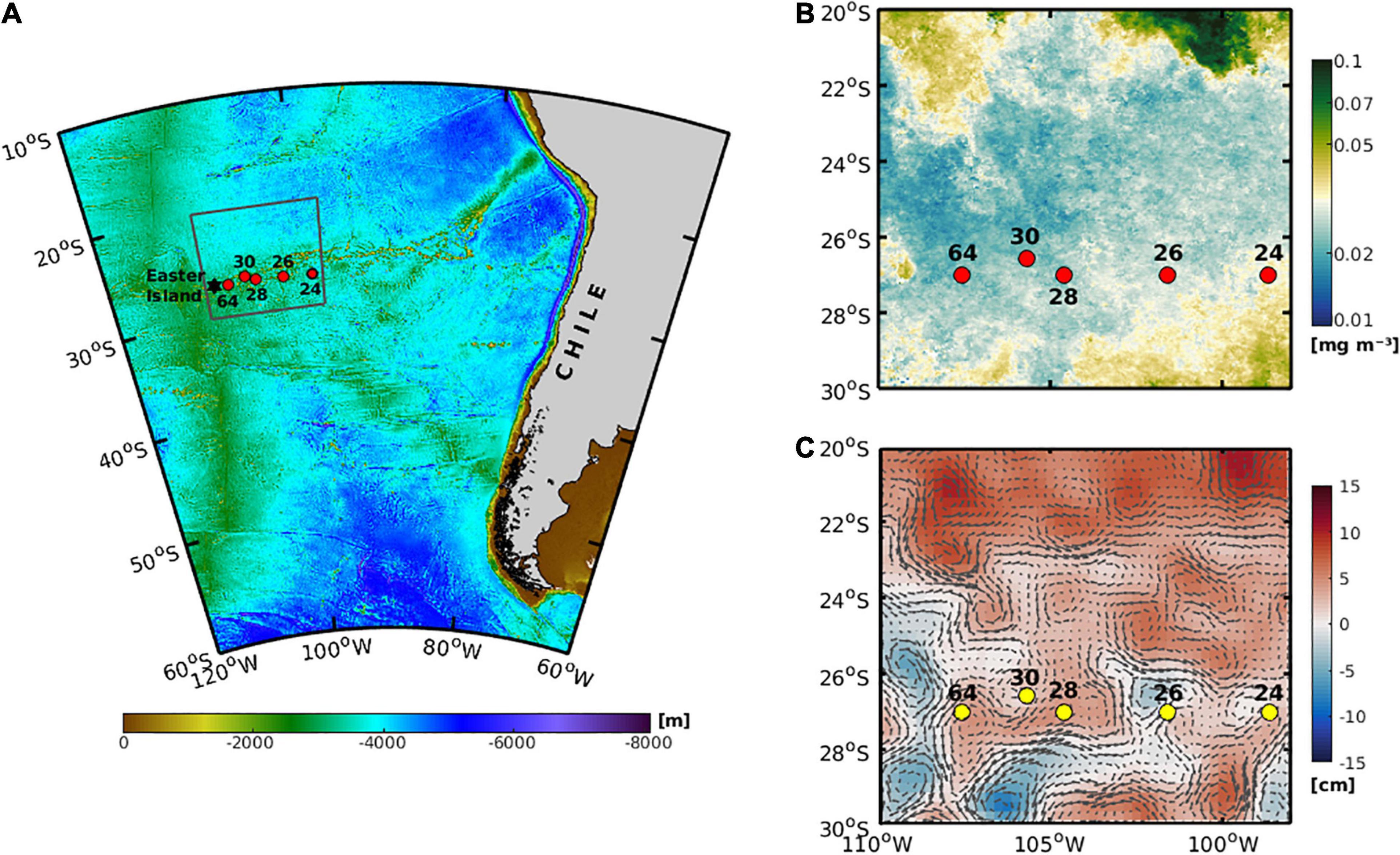
Figure 1. (A) Study area illustrating the stations for oceanographic data and zooplankton samples in the cruise CIMAR21 during October–November 2015 in the Pacific Southeast of Chile (∼27°S). (B) Monthly satellite-derived total Chlorophyll-a (mg m–3). (C) Sea level anomaly (cm) and the geostrophic velocity field.
Analysis of Oceanographic Data
In order to characterize the near surface bio-physical features, delayed-time sea level anomaly (SLA) from the satellite data was used to represent the geostrophic velocity field for the cruise period (October to November 2015). These data were obtained from the Salto/Duacs AVISO altimetry product1 for 0.25° × 0.25° grids of the central Chile region (20°S–30°S, 98–110°W). Monthly satellite-derived total Chl-a for the study region and for the same period was obtained from version 3.0 of the Ocean Colour Climate Change Initiative (OC-CCI2), at processing level 3 and a spatial resolution of 4 km. In addition, the total Chl-a data for each sampling station and for the five depth layers (0–100, 100–200, 200–400, 400–600, and 600–800 m) were obtained from a global biogeochemical reanalysis product from the Copernicus Marine Environment Monitoring Service (CMEMS; GLOBAL_REANALYSIS_BIO_001_0293).
Field data with regard to temperature, salinity, and dissolved oxygen from the oceanographic cruise were processed with the Gibbs Sea Water (GSW) Oceanographic Toolbox of TEOS-10 (IOC et al., 2010). The vertical profiles of these oceanographic variables were made with the Ocean Data View program. Conservative temperature and absolute salinity were derived from the CTDO, and T-S diagrams were made to identify the water masses. Finally, with the Optimum Multi-parameter (OMP) classical analysis in MATLAB software, we obtained the percentage of contribution of each water mass in the study area (Karstensen and Tomczak, 1999; Karstensen, 2020). Therefore, we used the interactive mode and characteristic water types (Table 1). To improve the water mass selection, the depth range was restricted to the following layers: 0–500, 300–700, and 400–1000 m. The analysis was carried out for each range of depth, and the type values of the water masses were assigned. Subsequently, the three ranges were joined and overlapped on purpose to find the scope of each mass. The data were extracted and plotted in the Ocean Data View Program version 5.2.1.
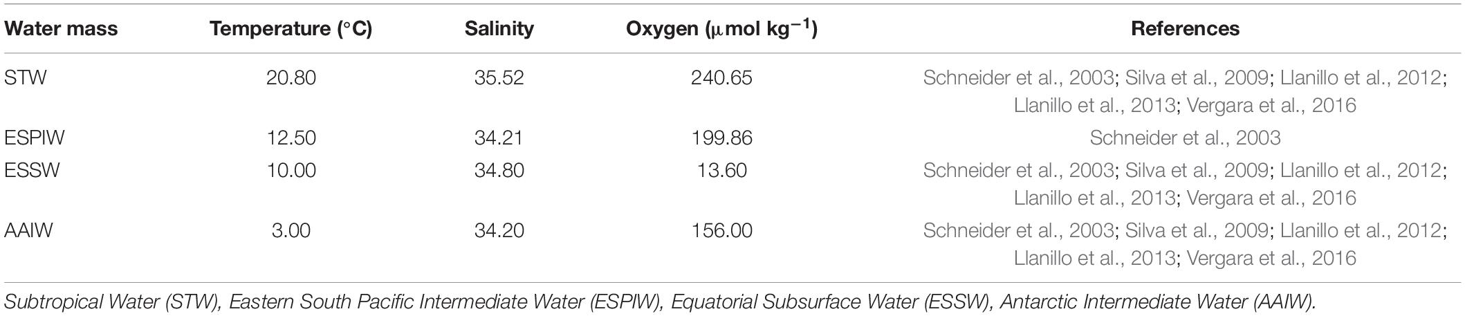
Table 1. Source water types used for the basic OMP analysis.
Descriptive statistics (means and range of variations) was obtained for oceanographic data. We grouped oceanographic data according to longitude and depth by using the ordination method of principal coordinates analysis (PCO), based on Euclidean distance with standardized data using PRIMER7 and the PERMANOVA+ add on. The PCO analysis placed the samples onto Euclidean axes using a matrix of inter-points dissimilarities, calculating the distances between centroids for the levels of a selected factor (Anderson et al., 2008). After using the PERMANOVA+ routine, the statistical differences of the environmental variables between depth layers (i.e., stratum and water mass) and longitude were tested.
Biological Data
Composition, Abundance, and Diversity
The composition of species was compared with the global database of the diversity and geographic distribution of marine planktonic copepods in the South Pacific Ocean. In particular, it was compared with the areas associated with the SPSG, such as the Central Tropical Pacific (Zone 19), the waters in front of Chile (Zone 26), and the waters around Australia (Zone 18), following the areas defined in the copepods database of Razouls et al. (2005/2019). To assign a few ecological attributes of the species present in the systematic list, horizontal distribution in the South Pacific Ocean (East and West coast and open ocean), vertical position in the column water (epipelagic, mesopelagic and bathypelagic), and trophic behavior (omnivorous, carnivorous, herbivorous) were extracted from this database, which complemented the data from the literature.
The abundance (N), species richness (S), and diversity indices of Shannon-Wiener (H′) and Simpson (1- λ′) were analyzed using descriptive statistics (mean, ranges and variation).
The indices used the following equations:
Where H′ = Shannon diversity index, pi = the proportion of each i species, and s = total number of species. 1-λ′ = Simpson diversity index, ni = the number of individuals of species i, and N = total number of species.
The Shannon-Wiener index ranges between 1 and 5, and the Simpson index ranges between 0 and 1. In this study, we decided to use both indices. Although the first index is more common in ecological studies, it is much more dependent on sample size and on a logarithm base for comparisons, whereas the second index is recommended as a measurement of the species of dominance (also reflecting diversity), independently from sample size (Lande, 1996; Gray, 2000; Lande et al., 2000). With the univariate data of abundance, richness, and diversity, “box and whisker” plots were constructed for graphical inspection, using PERMANOVA+, PRIMER7 software (Clarke and Gorley, 2006). With these community descriptors, we performed a non-parametric analysis of variance (Kruskal-Wallis) for testing the differences of the abundance (N), richness (S), and diversity indices (H′ and λ′) among depth strata and longitude representing the location of the stations.
Moreover, the presence/absence of species data was used to calculate two additional indices for taxonomic diversity: the average taxonomic distinctness (Δ+) and variation in taxonomic distinctness (Λ+). These indices show an average and an expected deviation for the study zone, when compared with the inventory of 546 species registered for the Central Tropical Pacific (Zone 19) by Razouls et al. (2005/2019). With the list of found species, a taxonomic aggregation matrix was made at the class, order, family, genus, and species levels. Thereafter, in the PRIMER7 program, with the TAXDTEST routine, the aggregation matrix was organized, and a classification tree was built from a random selection (n = 1000) of species from the general species inventory. Thus, comparing the indices and establishing confidence were limited to 95%.
The average (3) and variation (4) in taxonomic diversity are defined according the following equations:
Where the double summation is applied over all species i, j. N is the species number in the sample, and ωij is the assigned taxonomic path length of branch between i and j species (Clarke and Warwick, 1998). Λ+ is the variance of the taxonomic distances (ωij) between each pair of species i and j from their mean value (Δ+).
Copepods Community Analysis
Multivariate analyses of the copepod community were conducted with PRIMER7 and PERMANOVA+ add on software (Anderson et al., 2008). The data were transformed with log x+1 according to the Power Law of Taylor for aggregated data (Taylor, 1961). Thereafter, a similarity matrix for multivariate analysis of the composition and abundance was built. We first applied a cluster analysis using the Bray-Curtis index and average linking method and an ordination analysis of nonmetric multidimensional scaling (nMDS). Two factors were examined: longitude effects (98–110°W) and depth effects (five levels). The ANOSIM and permutational multivariate analysis of variance (PERMANOVA+) routines were applied to test these effects upon the hypothesis that community composition and the abundance of copepods did not differ significantly between a short range of longitude, but that they certainly differed between depth strata, considering the distribution of water masses. In the PERMANOVA+, the factor levels of depth and longitude (stations) were pooled as duplicates to assess the individual effect of each single factor. Since no differences in abundance, richness, or diversity of copepods were found (Kruskal-Wallis test P > 0.05, Supplementary Table 7), the day/night factor was not considered for these multivariate analyses. Thereafter, the differences or similarities between groups were analyzed with the SIMPER module (similarity percentages), with the aim of finding the contribution of individual species to similarity or dissimilarity between the analyzed groups. We also calculated the weighted mean depth (WMD) or gravity center for species with the highest contribution from SIMPER analysis:
Where di is the depth of a sample i (center of the depth interval), zi is the thickness of the stratum, and ni is the number of individuals per 100 m3 at that depth (Worthington, 1931; Roe et al., 1984; Andersen et al., 2004). When vertical distribution of a species was bimodal, WMD was calculated for two portions of the water column (surface = 0–200; deep = 200–800 m).
Finally, the biological and environmental (BIOENV) analysis based on Spearman’s correlation matrix was used to determine which oceanographic variable (temperature, salinity, oxygen, and Chl-a) affected the abundance and distribution of copepods. The biological data matrix was log (x+1) transformed, and the oceanographic data was normalized (subtracting the mean and dividing by the standard deviation for each variable). To determine whether the composition and abundance of zooplankton were related to oceanographic variables, a distance-based redundancy analysis (dbRDA) and a distance-based linear model (DistLM) (Clarke and Warwick, 2001; Clarke and Gorley, 2006; Anderson et al., 2008) were performed. DistLM uses permutation methods to test the plausibility of the null hypothesis (i.e., no relationship between the resemblance matrix of the principal component scores of zooplankton data and one or more environmental predictor variables). To find the best explanatory model from all possible combinations of the predictor variables, the analysis followed a stepwise procedure selection (Anderson et al., 2008) and the Akaike’s information criterion (AIC) (Akaike, 1973). The smallest achieved value of AIC indicated the best model, i.e., the best combination of the environmental predictor variables that explains the largest amount of variation in the response variable (copepods species). Additionally, further marginal tests can account for the percentage of variance of copepods when each environmental variable is considered individually through a Pseudo-F value, which is a direct multivariate analog of the Fisher’s F ratio used for standard analysis of variance. Moreover, we used a multiple linear regression model to evaluate the relationship between the total abundance, richness, and diversity indices (Shannon-Wiener and Simpson) of copepods and environmental variables (Temperature, Salinity, Oxygen, and Chl-a). Multicollinearity between variables was tested with a multiple Spearman correlation, temperature and salinity were treated separately due to their high correlation (R > 0.97) (Supplementary Table 6).
Results
Bio-Physical Near-Surface Features and Oceanographic Characterization
The total Chl-a concentration in the study area, located between 2800 and 3800 km from the coastal zone of Chile, during October and November of 2015 was extremely low, with mean values lower than 0.1 mg m–3 (Figure 1B). The sea level anomaly and estimated geostrophic currents derived from satellite information showed a moderate to low level of eddy kinetic energy (EKE), prevailing positive or zero SLA values around the sampling stations (Figure 1C), contrasting with the observed patterns described in the coastal zone with higher EKE activity (Hormazabal et al., 2013).
The vertical profiles of temperature and salinity between 0 and 800 m showed a highly stratified water column. High temperature values (ca. 20°C) in the upper layer (0-∼150 m) delimited the mixed layer, below which the temperature decreased to 7°C at the depth of 450 m, defining the permanent thermocline. Between 450 and 800 m depth, the temperature decreased uniformly down to 5°C (Figure 2A). The salinity showed high values (35.5 – 36.0) in the upper layer, down to approximately 150 m depth, after which it decreased rapidly to 34 at 350 m, maintaining this value down to 800 m depth (Figure 2A).
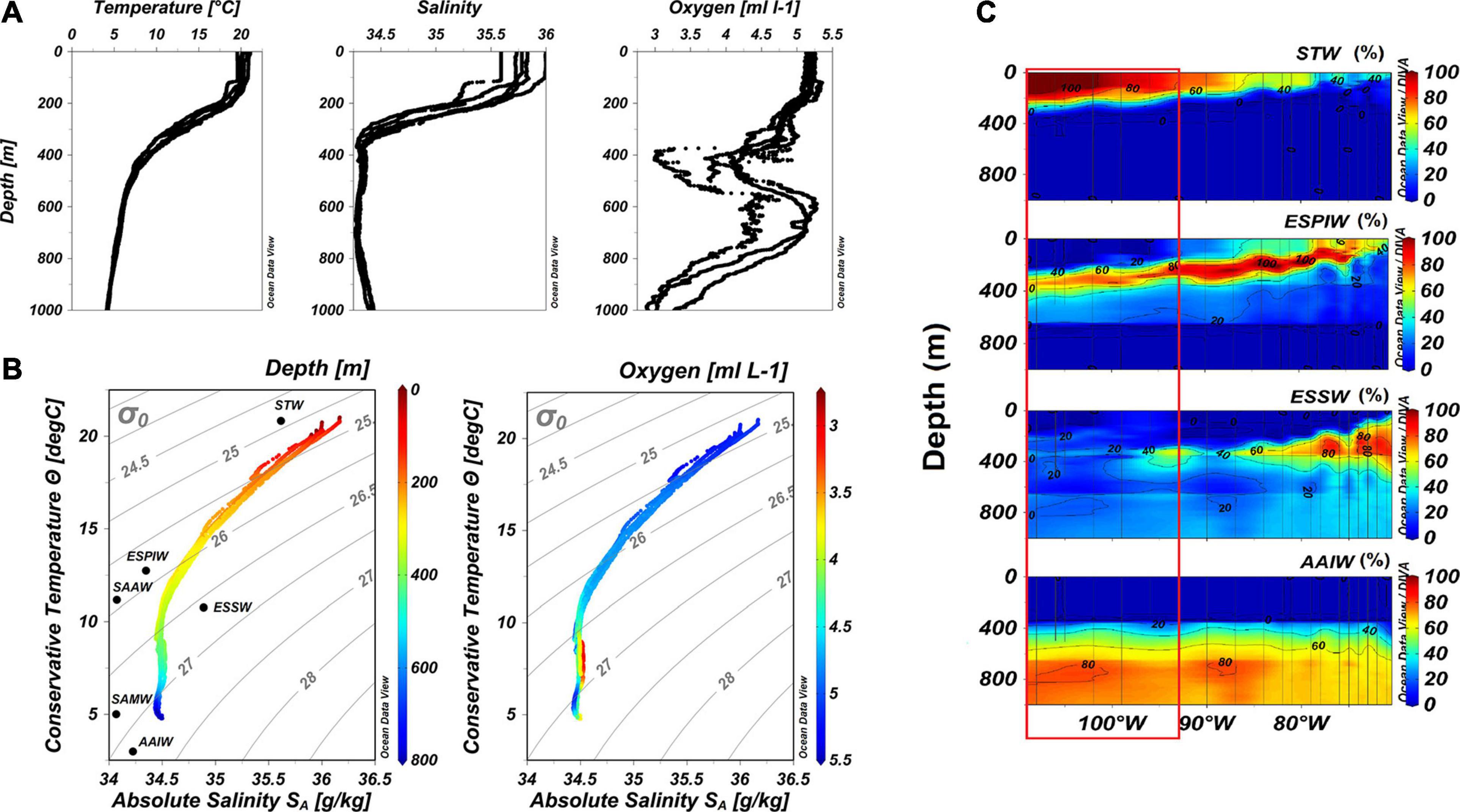
Figure 2. Oceanographic characteristics in the SPSG and over the coastal-oceanic transect of the CIMAR-21 cruise showing the water masses contribution (%) in the Pacific Southeast, Chile, (∼27°S) during October and November of 2015. (A) Vertical profiles of temperature, salinity and oxygen of the water column in the SPSG (98–110°W). (B) T-S diagram in the SPSG (98–110°W), left by depth and right by oxygen concentration. (C) Contribution in percentage of water masses in the Pacific Southeast of Chile longitude 70–110°W; the red rectangle shows the study area in the longitude 98-110°W. Subtropical Water (STW), Eastern South Pacific Intermediate Water (ESPIW), Equatorial Subsurface Water (ESSW), Antarctic Intermediate Water (AAIW).
The water column was well oxygenated at most depths (∼5 ml L–1), and the highest concentrations of oxygen were found between the surface and 350 m depth. Thereafter, oxygen declined in the layer between 350 and 500 m (Figure 2A). In four stations, the oxygen decreased down to 3.7 ml L–1, and one station (98°W) showed the lowest value (2.98 ml L–1). From 500 to 750 m depth, the oxygen increased again up to 5 ml L–1, although the station located at 98°W showed a different pattern, where oxygen increased up to 4.5 ml L–1. Below 750 m depth, the oxygen decreased to ∼3 ml L–1 (Figure 2A). Predominantly, this vertical profile is a characteristic for signaling the presence of a potential intra-thermocline anticyclonic eddy (ITE; Hormazabal et al., 2013; Cornejo D’Ottone et al., 2016). Complete data on oxygenation of the water column can be found in the oxygen section reported as Supplementary Figure 1.
In the SPSG at 27°S, in oceanic waters, between 98 and 107°W, the T-S diagram and OMP analysis showed four water masses: Subtropical Water (STW) with 100% of contribution between 0 and 200 m depth, the Eastern South Pacific Intermediate Water (ESPIW) with 60–80%, the Equatorial Subsurface Water (ESSW) with 20–40% at 200–400 m depth, and the Antarctic Intermediate Water (AAIW) with 20–60% between 400 and 600 m and 80–100% of contribution at 800–1000 m depth (Figures 2B,C).
Regarding the environmental variables, the PCO analysis allowed us to distinguish some clusters associated with depth (Supplementary Figure 2). The PCO1 and PCO2 components explained 98.82% of variability in the oceanographic data (temperature, salinity, and oxygen). Three groups were differentiated. The first group represented all the stations from the upper stratum between 0 and 200 m, the second group had data of the intermediate stratum between 200 and 400 m depth, and a third group had the data of the deeper strata (400–600 m and 600–800 m depth). The scatter plot of the second group had a minor distance with the third group (deep) as compared to the first group (upper), indicating that the environmental characteristics of the second group (200–400 m) are more similar to those of deep waters, as compared to those of the surface layer.
Composition of Species
A total of 121 species of copepods were found in the SPSG, and some collected species are shown in Figure 3. These species belong to five orders, 24 families, and 50 genera (Figure 4 and Supplementary Table 2). The orders Calanoida and Cyclopoida were the most represented, with 57% and 38% of the species, respectively, whereas Harpacticoida and Mormonilloida were represented with 2% of the species each, and Siphonostomatoida was represented with 1% of the species. Cyclopoida showed a higher proportion than Calanoida in the upper layer (0–200 m) but this proportion changed below 200 m depth, with an increase in Calanoida and the appearance of other orders, such as Harpacticoida and Mormonilloida (Figure 4).
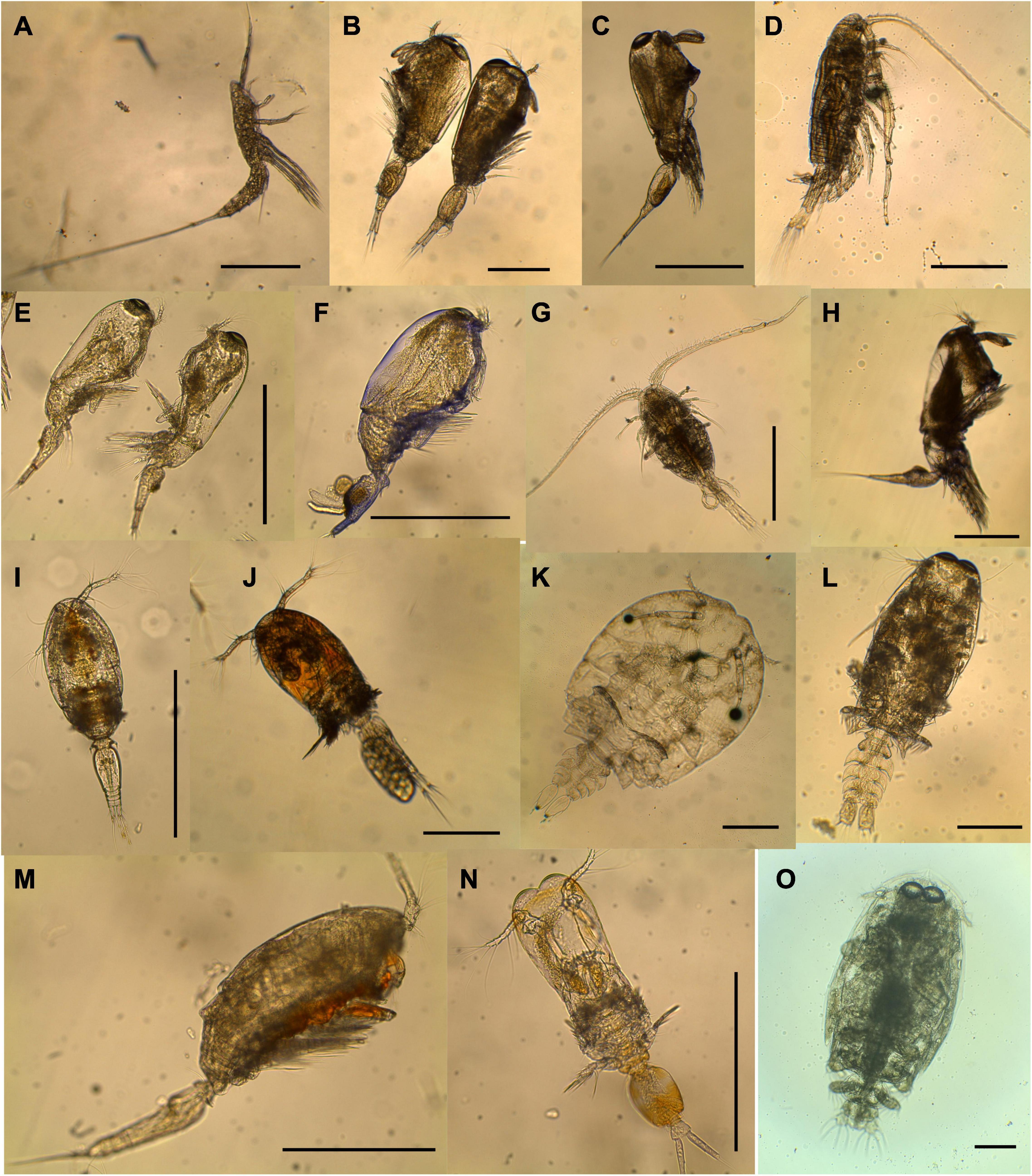
Figure 3. Examples of common species of copepods collected during October to November 2015 in the SPSG. (A) Aegisthus mucronatus, (B) Agetus limbatus, (C) Agetus typicus, (D) Centropages brachiatus, (E) Farranula curta, (F) Farranula gibbula, (G) Lucicutia gaussae, (H) Monocorycaeus robustus, (I) Oncaea media, (J) Oncaea mediterranea, (K) Sapphirina intestinata, (L) Sapphirina metallina, (M) Triconia conifera, (N) Vettoria parva, (O) Order Siphonostomatoidea (Familiy Pandaridae). The black scale is 500 μm.
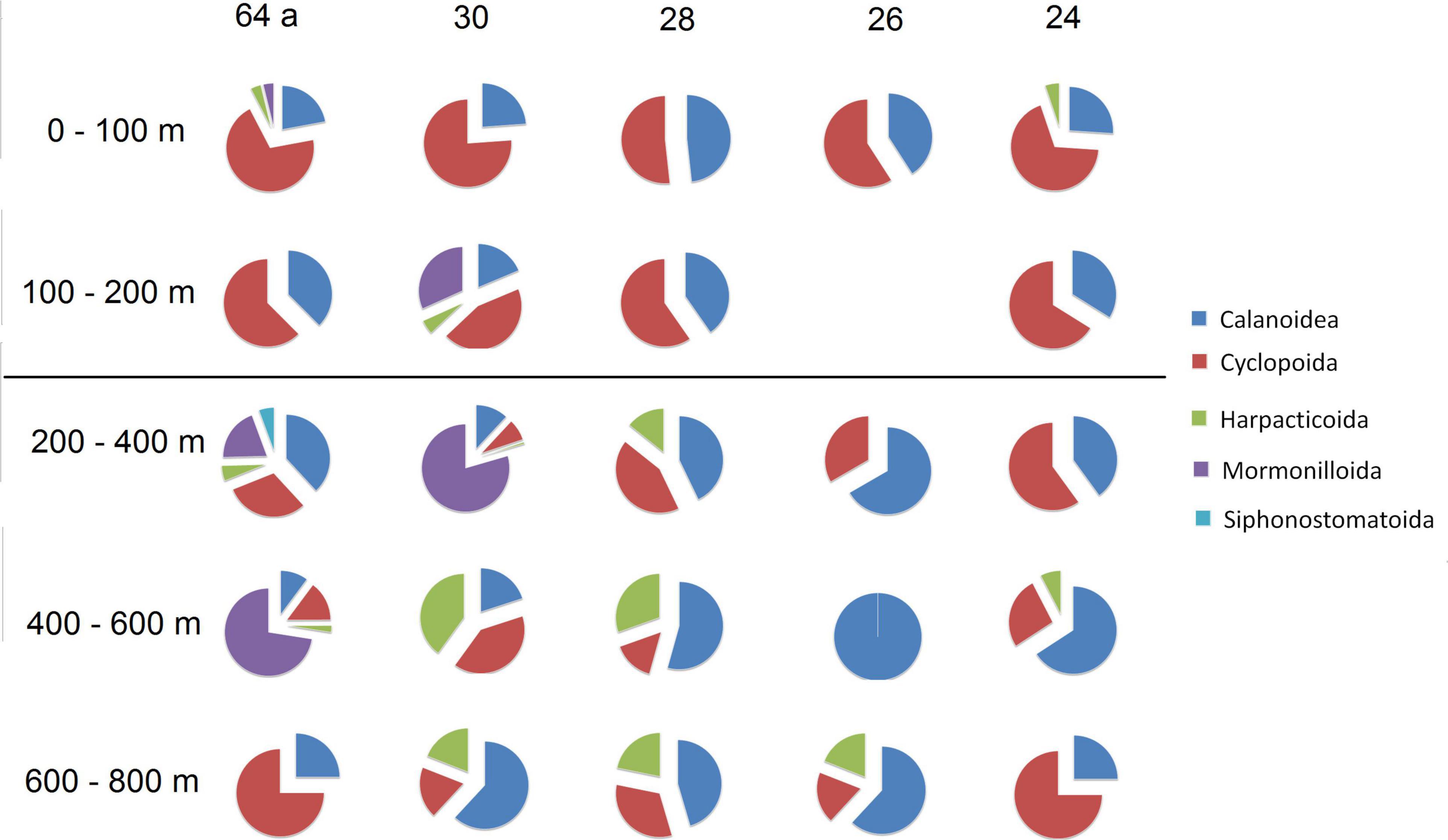
Figure 4. Pie charts to illustrate the distribution of orders of the subclass Copepoda in five stations and different depth strata in the oligotrophic water of the south Pacific subtropical gyre during the CIMAR-21 cruise (October–November 2015).
In the order Calanoida, the families with most species were Clausocalanidae (12), Aetideidae (9), Paracalanidae (8), and Metridinidae (7). The most abundant calanoid genera were Clausocalaus, Pleuromamma, Paracalanus, and Lucicutia. In Cyclopoida, the families were Corycaeidae (17), Oncaeidae (10), and Sapphirinidae (10). The most abundant copepods were the genera Corycaeus, Farranula, Oithona, Oncaea, and Sapphirina.
According to Razoulz et al. (2015/2018), 62% of these species exhibit a wide geographic range in the South Pacific Ocean, with 15% occurring in the oceanic South Pacific zone and West coast, while only 4% can be found in oceanic and coastal zones (East and West). Regarding the vertical distribution, 34% of the species were found in the epi- and mesopelagic depths, 25% were discovered only in the epipelagic zone, 19% were found in epi-, meso-, and bathypelagic depths, and 6% were observed in meso- and bathypelagic depths. However, 13% of these species did not show a clearly defined vertical habitat. On the other hand, the ecological role of copepods species of SPSG was assessed by assigning the feeding habits of various species in accordance with Benedetti et al. (2016). From the 121 species found in the SPSG, it may be stated that 21% of the species exhibit omnivorous and herbivorous behaviors, while 17% are omnivorous, 14% are carnivorous, and 10% are omnivores and detritivores. However, 36% of the species remain unknown (Figure 5).
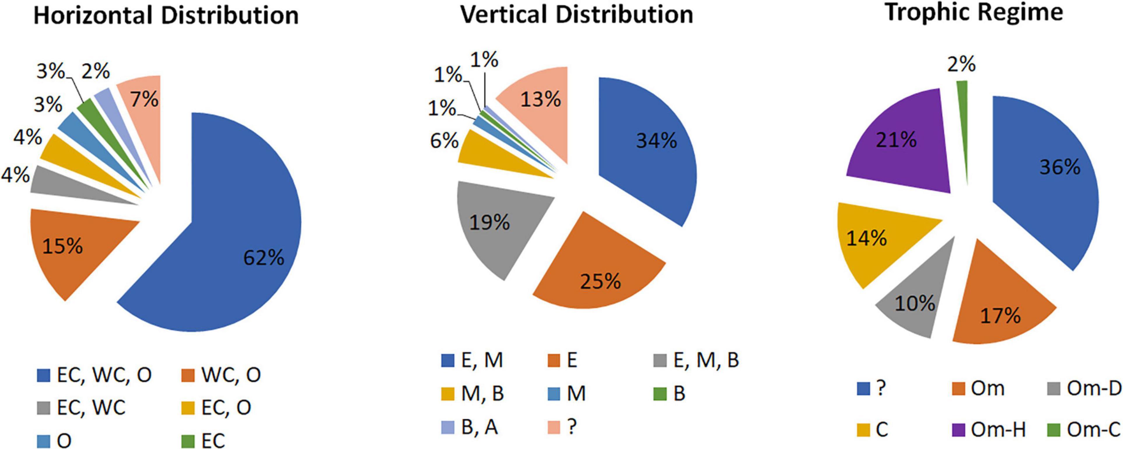
Figure 5. Pie charts showing the horizontal and vertical distribution of pelagic copepods in the South Pacific Ocean (EC = East Coast, WC = West Coast, O = Oceanic; E = Epipelagic, M = Mesopelagic, B = Bathypelagic, A = Abisopelagic) and trophic regime (Om = Omnivore, D = Detritivore, H = Herbivore, C = Carnivore (Razouls et al., 2005/2019; Benedetti et al., 2016).
Abundance and Diversity of Copepods
In the oceanic zone, total copepods abundance ranged between 6 and 3000 ind. 100 m–3, with a mean of 570 ind. 100 m–3 (Figures 6A,B and Supplementary Figure 3). The mean richness by station was 15 species, with a maximum of 36 (E:64A, 105 W, stratum 0–100 m) and a minimum of two species (E:26, 101 W, stratum 400–600 m) (Figures 6A,B). The diversity index of Shannon showed a mean of 1.90, and the highest value was 3.80 (E:28, 104 W, stratum 100–200 m), while the lowest was 0.81 (E:26, 101 W, stratum 400–600 m). The range of variation of the Shannon index indicates that changes in species composition can strongly vary over space, revealing a heterogeneous copepod community, although most variance was accounted for by depth stratum. The Simpson index, on the other hand, indicates the degree of dominance by a single species. The average Simpson index was 0.78, with a range of 0.91–0.42 (E:26, 101 W, stratum 0–100 m and E:26, 101 W, stratum 400–600 m, respectively) (Figures 6A,B). This range shows a low level of dominance and a high level of diversity, especially in surface waters (0–100 m). However, diversity and abundance significantly decreased with depth, and the two epipelagic strata (0–100, 100–200 m) showed the highest abundances and species richness and diversity compared to the deepest layer (200–400, 400–600, and 600–800 m) (Figure 6B). Over the longitude axis, low variability was found without significant differences in abundance, richness, and diversity. In contrast, depth strata showed significant differences (Table 2).
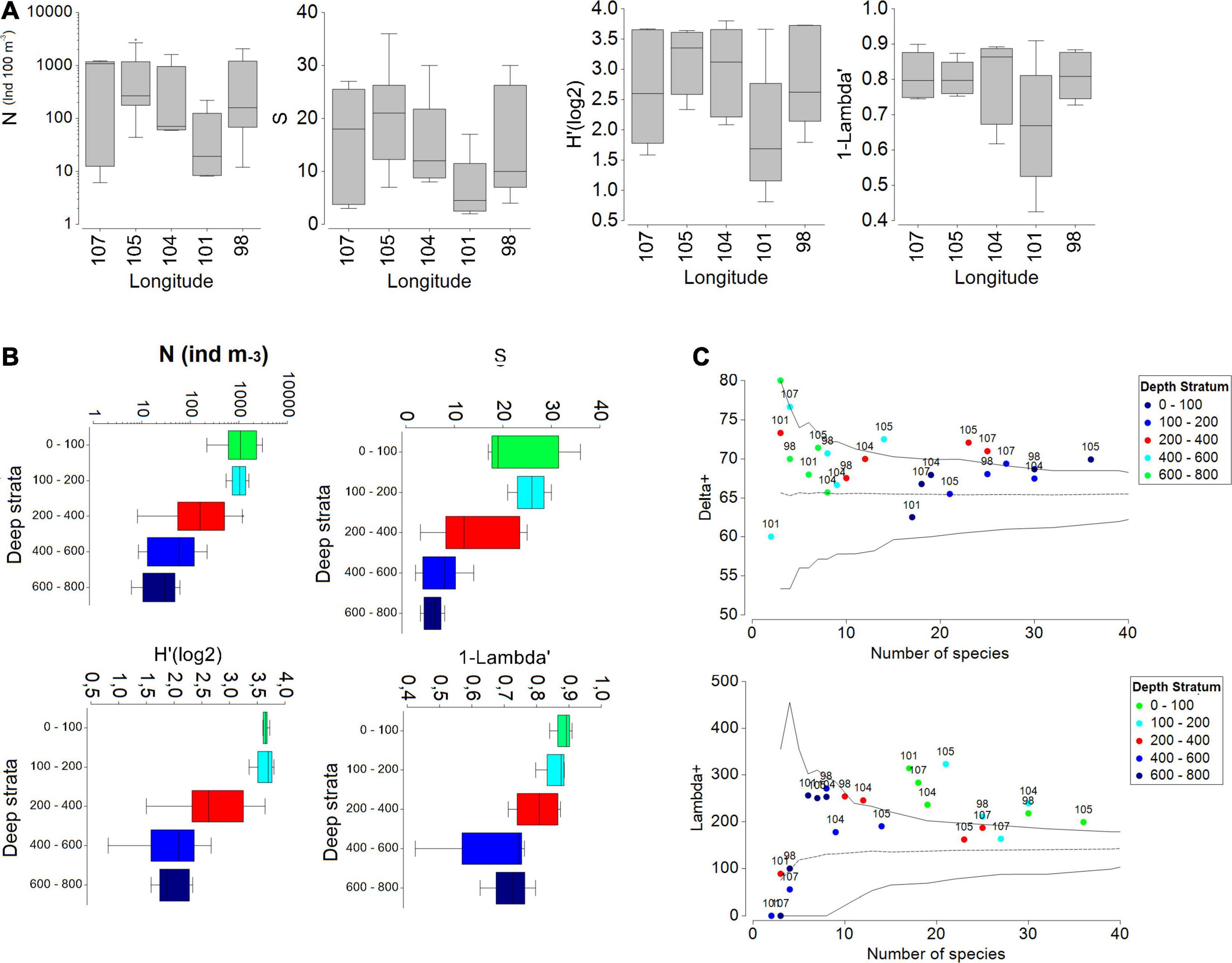
Figure 6. (A) Boxplot of abundance (N, log scale), richness (S) and diversity index (Shannon-Wiener and Simpson) of the copepod community in the Pacific Southeast, Chile, (∼27°S) during October and November of 2015 by longitude. (B) Boxplot of the same biological descriptors by depth strata and the boundary of the box indicates the 25th and 75th percentile, the line within the box indicates the median, and the whiskers above and below the box indicate the 90th and 10th percentile. (C) Average taxonomic distinction index (delta+) and average taxonomic variation index (lambda+) for the copepod community in the SPSG. The central line shows the mean, while the continuous lines are the distribution of probability at 95%.
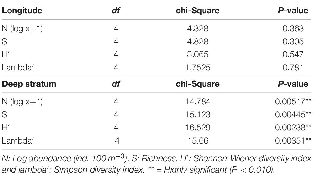
Table 2. Kruskal-Wallis to test the influence of longitude and depth stratum on abundance, species richness, and diversity of copepods in the SPSG.
With the inventory of 541 species of copepods recorded for the oligotrophic zones in the Pacific Ocean (Razouls et al., 2005/2019) and the list of 121 species identified in this study, the average and variation taxonomic distinctness (delta and lambda+) shown in the funnel plot (Figure 6C) were calculated. Generally, the taxonomic distinctness (delta+) values fell within the 95% confidence limits, indicating that the copepod community contained the expected level of species diversity for the region, albeit with high variability. The taxonomic distinction index (delta+) had an expected mean of 65, and the expected taxonomic distinction variation (lambda+) had a value of 100 (Figure 6C). In the delta+, the highest value was found at 107°W at 400–600 m depth, while most samples were greater than average, with only two falling below average (Figure 6C). The lowest values were observed at 101°W at the 0–100 and 400–600 m depth layers. The most oceanic stations (107°W and 105°W), especially in the 200–400 and 400–600 m depth layers, fell outside and above of the confidence limit, showing that average taxonomic distinctness was higher than what was randomly expected. Moreover, in the lambda+, all the stations of the upper layer (0–100 m) and three stations (105, 104, and 98°W) of the second surface layer (100–200 m) were found outside and above the confidence limit, thus displaying a much higher variability (Figure 6C).
Multivariate Analysis and Environmental Correlates
Five groups with 20% similarity (80% dissimilarity) were found. One group was formed with the two first levels of depth (0–200 m), along with some samples of the third strata at 200–400 m of depth. Four groups with stations were formed with the last two levels of depth (400–600 m and 600–800 m) (Figure 7A). The similarity analysis (ANOSIM) showed significant differences in the composition and abundance of copepods by depth stratum (R = 0.398, p-Value = 0.005). No differences were found by longitude (R = 0.104, p-Value = 0.198). The main differences by depth were found between the deepest and shallowest strata (i.e., 400–600 m and 600–800 m vs. 0–100 m and 100–200 m). The intermediate stratum (200–400 m) showed differences with the shallowest stratum (0–100 m) (R = 0.556, p-Value = 0.008), but not with the second (100–200 m) or the deepest (400–600 m and 600–800 m) (R = 0.174, p-Value = 0.095 and R = 0.136, p-Value = 0.159), even though the second fell on the rejection limit (R = 0.238, p-Value = 0.056).
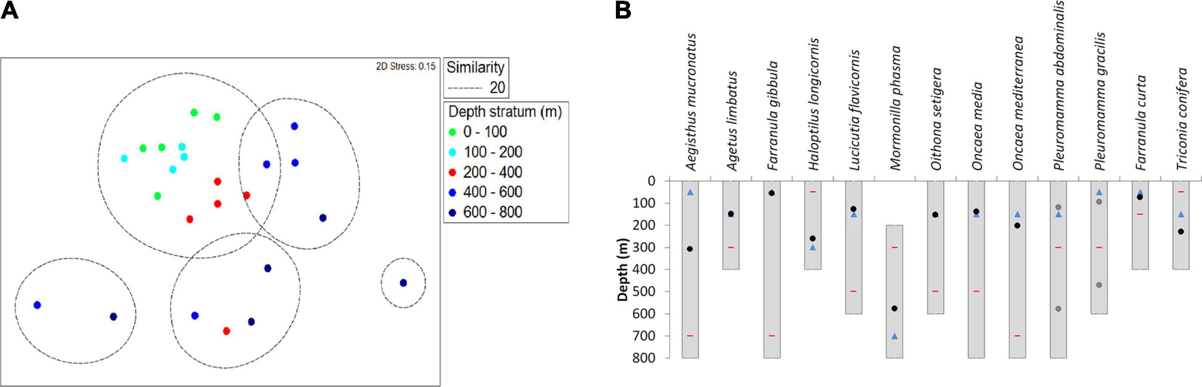
Figure 7. Multivariate analysis of the composition and abundance of copepods species in the SPSG (∼27°S) during October–November 2015. (A) Non-metric multidimensional scaling (nMDS) plot on the first two axes based on the Bray-Curtis similarities of the log (x+1) of transformed copepod species abundance data for depth strata. (B) The weighed vertical distribution (WMD) for species selected by SIMPER analysis (black dot), depth stratum with the lowest abundance (red stripe), depth for the highest abundance (blue triangle), and WMD for species with bimodal distribution (gray dot).
In the percentage similarity analysis (SIMPER), the composition and abundance of copepod species showed a higher average value of Bray-Curtis dissimilarity (70–95) than of similarity (8–32) (Supplementary Tables 3, 4). The average of similarity decreased with depth, being higher in the first two strata (32.47 and 32.88). The species with the highest percentage of contribution were Lucicutia flavicornis and Farranula gibbula in the first stratum (0–100 m) and Oithona setigera and Oncaea media in the second (100–200 m). The intermediate stratum (200–400 m) showed an average similarity of 24.50, and the most important species were Haloptilus longicornis, Oncaea media, and Oncaea mediterranea. In the deepest strata, with an average Bray-Curtis similarity of 11.25 (400–600 m) and 8.02 (600–800 m), the species with the highest contribution were Pleuromamma gracilis and Aegisthus mucronatus at the depth of 400–600 m and Mormonilla phasma and Oncaea media at the depth of 600–800 m (Supplementary Table 3).
A high level of dissimilarity in the community structure among depth strata was found (Supplementary Table 4). However, seven dominant species reached a higher percentage of contribution (38–32%), especially between the upper (0–200 m) and the deeper strata (600–800 m). The contribution of single taxa to spatial dissimilarity was relatively low (<8.5%), suggesting that changes in abundance can occur rather than changes in presence/absence of species, thereby explaining the high level of dissimilarity between the depth layers (Supplementary Table 4).
The vertical distribution of 13 species selected by SIMPER analysis revealed that five species occurred at all depth strata (Aegisthus mucronatus, Farranula gibbula, Oncaea media, O. mediterranea, and Pleuromamma abdominalis; Figure 7B). Three species occurred between 0 and 600 m depth (Oithona setigera, Lucicutia flavicornis, and Pleuromamma gracilis), four species were restricted to the upper 400 m of the water column (Corycaeus (Agetus) limbatus, Haloptylus longicornis, Farranula curta, and Triconia confiera), and one species occurred only between 200 and 800 m depth (Mormonilla phasma) (Figure 7B).
However, the WMD or gravity center differed greatly. Only Farranula gibbula and F. curta had their WMD in the surface layer at around 50 m depth. Aegisthus mucronatus, Lucicutia flavicornis, Oithona setigera, Oncaea media, O. mediterranea, and Triconia conifera had a WMD near to 150 m. The mesopelagic distribution at 300 m depth consisted of Aegisthus mucronatus, Haloptylus longicornis, Pleuromamma gracilis, and P. abdominalis. The species with the deepest distribution was Mormonilla phasma (WMD ∼600 m) (Figure 7B and Supplementary Table 5).
The BIOENV analysis showed that the temperature presented the highest correlation value with the abundance of copepod species, with a value of 0.417, and the combination of the temperature and oxygen, with a correlation of 0.406. The relationship between the composition and abundance of copepods and the potential environmental drivers is visualized in the constrained dbRDA plot, with the first two axes explaining 24.34% of the total variation (Figure 8A). The first axis (17.4% of total variation) is related to the surface layer (temperature and salinity). The second axis (6.9% of total variation) is related to oxygen and the intermediate layer (200–400 m). Similarly, the DistLM sequential tests for the copepod community suggested that temperature was the best predictor variable (Pseudo-F = 4.6047, p = 0.001, AICc = 195.85), accounting for 17.3% of the total variation observed in the copepod community composition across five depth strata (Table 3). Figure 8B shows the DistLM results by means of a dbRDA plot, with the temperature retained by the procedure. The bubbles show the vertical gradient with higher temperature values in the shallow and intermediate strata (0–400 m) as compared to the deeper ones (400–600 and 600–800 m).
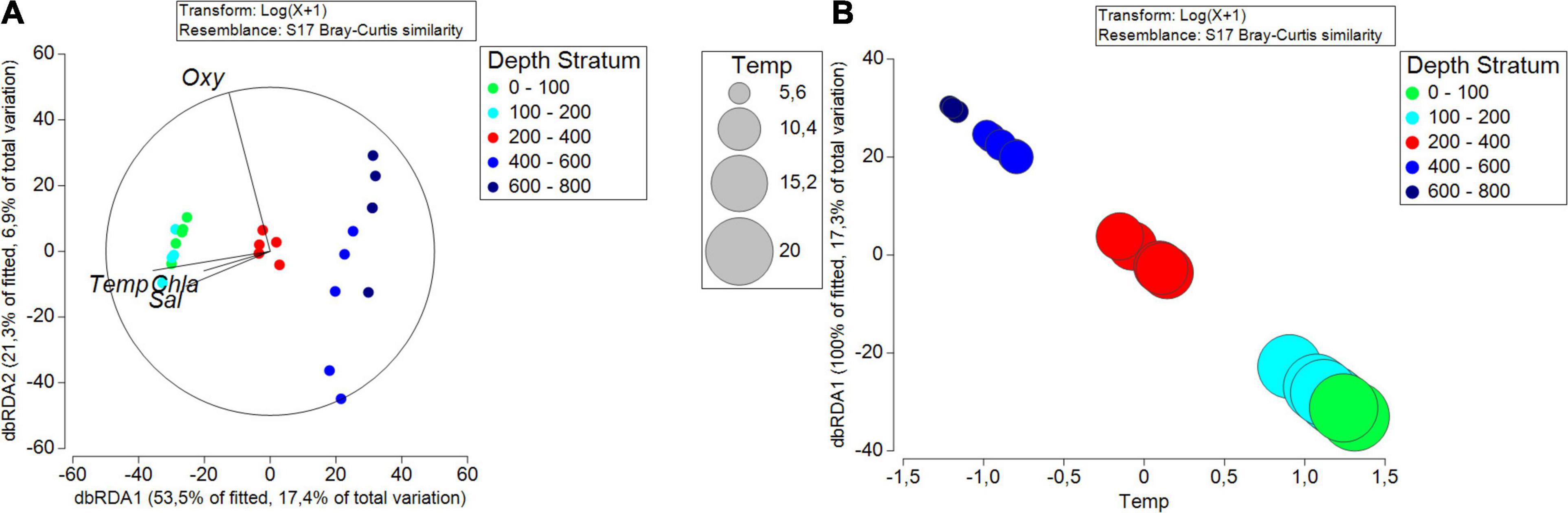
Figure 8. (A) The distance-based redundancy analysis (dbRDA) ordination plot relating the structure of the copepod community across the depth layers and stations. Data points indicate different study sites (SPSG), and their colors indicate the depth layer of samples. The length of each vector represents the importance of the oceanographic variable (Temp = temperature, Sal = salinity and Oxy = oxygen), while the direction shows the correlation with these samples, and the circle shows the threshold for a correlation = 1. (B) dbRDA bubble plot of the DISTLM sequential test showing temperature as the predictor variable to explain the variation of copepods community in the SPSG.
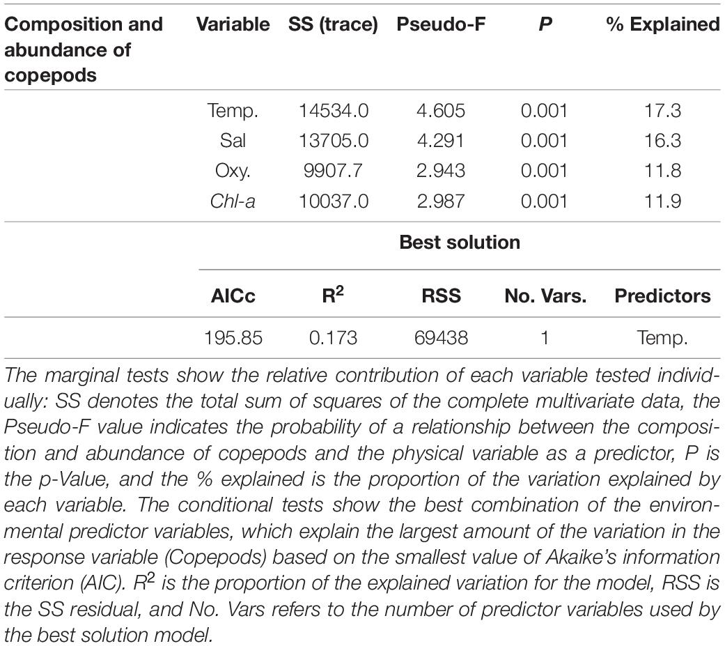
Table 3. Composition and abundance of copepods variance explained by the environmental variables in the SPSG through DistLM analysis.
When assessing the association of community descriptors (diversity indices and total abundance) with environmental variables, it was found that water temperature and salinity showed significant linear effects on the diversity indices and species richness in most cases, but not oxygen concentration or Chl-a (Figure 9). Temperature and salinity explained most of the variance of the diversity indices after a multiple linear regression model (Table 4). Temperature was the best predictor (R2 > 0.69), especially for the Shannon-Wiener diversity index (R2 = 0.75). The contribution of each environmental variable to the total variance of the community descriptors is shown in Table 4.
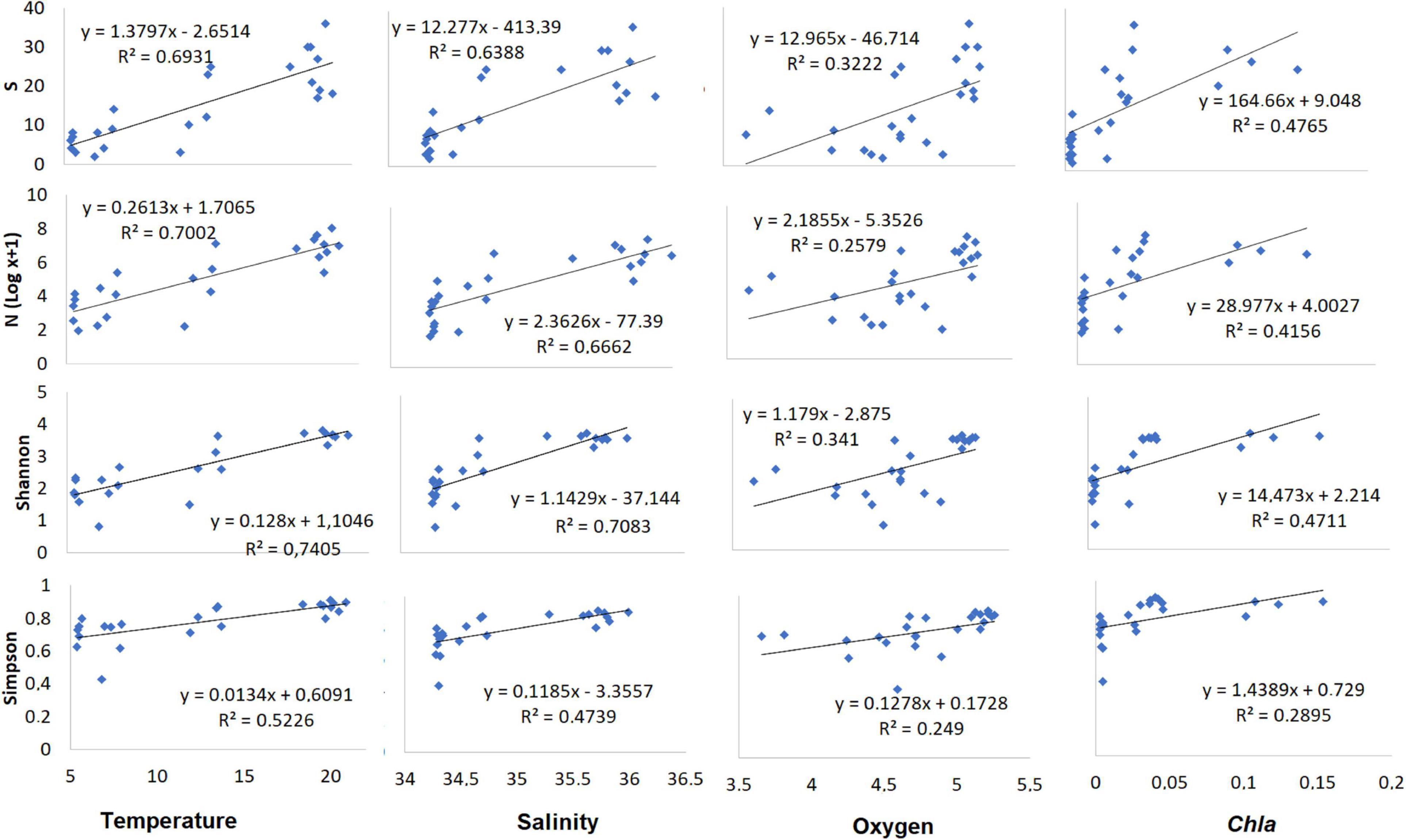
Figure 9. The relationship between species richness (S), abundance (log N), and the Shannon-Wiener (H′) and Simpson (λ′) indices of diversity of the copepod community in the SPSG during the austral spring of 2015 and environmental (bio-physical) drivers (temperature, salinity, oxygen, and Chl-a).
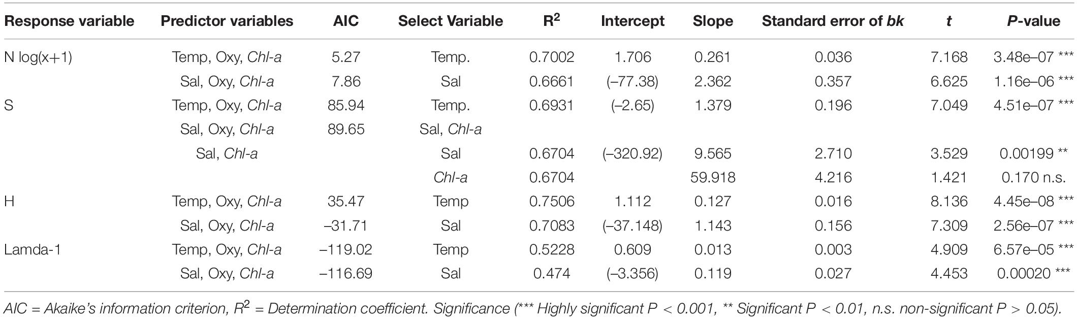
Table 4. Multiple linear regression (stepwise) to assess the relation between community descriptors (N = abundance, S = Richness, H = Shannon-Wiener diversity index and Lamda-1 = Simpson diversity index) and environmental conditions.
Discussion
Hydrographic Conditions in the SPSG
Three water masses have been previously registered in oceanic waters of the Southeast Pacific in the region located at 27°S and between 98 and 110°W: The Subtropical Water (STW), Antarctic Intermediate Water (AAIW), and the Pacific Deep Water (PDW) (Fuenzalida et al., 2007; Silva et al., 2009). As proposed by Silva et al. (2009), there are two water masses in this subtropical area, which may not extend beyond 95°W. The Sub-Antarctic Water (SAAW) extends offshore and occupies the upper 200 m, and the Equatorial Sub-surface Water (ESSW) advects westward in a similar fashion, but with its core centered at ca. 400 m depth at 95°W. However, according to our data, at a latitude of 27°S, the presence of SAAW was unclear, and it did not show a strong contribution in its characteristic layer (200–400 m) at the offshore area (95–108°W). SAAW did not coincide with the area either and suggested limits of its distribution for the Southeast Pacific (Llanillo et al., 2012). An additional water mass was later described for the region by Schneider et al. (2003); Hernández-Vaca et al. (2017). This is the Eastern South Pacific Intermediate Water (ESPIW), with its core in the subtropical convergence approximately at 33–38°S, between the Chilean coast, and at 90°W. This water mass is formed by subduction southeastward of the wind-driven gyre circulation, or subduction of SAAW forming the ESPIW, which continues advecting toward the equator following the direction of the Humboldt current system. ESPIW is located at 50–400 m of depth, and it spreads within the subtropical gyre as far as 150°W. In the present study, we confirmed the presence of the ESPIW water mass located at 200–300 m depth within 80–95°W and the deepest at 300–400 m in the SPSG (95–110°W).
The presence and contribution of the different water masses may also control prevailing conditions for near-surface and subsurface oxygenation at the SPSG. For instance, our vertical profiles of oxygen showed one of the stations (27°S, 98°W) with low concentrations of oxygen at depth (2–3 ml L–1). This low oxygen was also evident in the T-S-O2 diagram, indicating the contribution of the ESSW at the offshore region (20–40%). In fact, ESSW was present in the entire coast-ocean section, with a nucleus at 300–500 m depth, and became more evident in the coastal zone with a contribution of 40–50%. Recently, Cornejo D’Ottone et al. (2016) also registered low oxygen concentrations at the subsurface level (200–400 m) in oceanic waters (∼900 km from shore) in the southeastern Pacific (30°S, 81°W), associated with an anticyclonic intra-thermocline eddy (ITE), which exhibited properties linked to ESSW (Chaigneau et al., 2011). This ESSW in the coastal zone is the main source for the upwelling process, but it also forms the oxygen minimum oxygen zone (OMZ), whereas ITEs are mesoscale structures (10–100 km, months) that can transport heat, salt, and the physicochemical and biological properties of such ESSW toward the open ocean (Pizarro et al., 2006; Hormazabal et al., 2013; Cornejo D’Ottone et al., 2016). Therefore, the offshore advection of ESSW from the coastal zone driven by mesoscale eddies may also transport nutrients to the subsurface water of the SPSG, and this process may sustain some of the low primary production that has taken place at the deeper depths of the euphotic zone. Although the primary production remains low, this can provide food resources for the highly diverse copepod community at the SPSG.
Composition of Copepods in the SPSG
This study provides the first glimpse at the copepod community composition in the SPSG, identifying 121 species. This number should be considered high, provided that only a few locations were sampled compared to the records from the coastal zone of north and central-south of Chile, where 76–118 species have been identified (Hidalgo et al., 2010; Fierro, 2014; Pino-Pinuer et al., 2014). However, it is relatively low when compared to the global database of the diversity and geographic distribution of planktonic marine copepods, in which 546 species of copepods have been registered for the oceanic zone of the Pacific, an extensive area named as the Central Tropical Pacific (Zone 19), which includes the North Subtropical Gyre, the tropical area with the north and south equatorial countercurrent, and the South Subtropical Gyre. However, when focusing solely on the SPSG, as one of the most unexplored areas of the ocean, 122 records of epipelagic species of copepods have been reported for the western zone (155°W). These data come from cruises in the 1960’s, and were published by Williamson and McGowan (2010). The number of species is similar to those found in our study in the eastern zone (121 species), although the data cannot be easily compared due to different sampling methods, such as larger mesh size (505 μm) and a different sampling gear that may sample another type of community (macrozooplankton).
Another comparable region is the North Pacific Central Gyre. In this region, a considerably high sampling effort has been invested in the ALOHA’s time series, in which the richness of species shows a value of 158 species within the North Pacific Gyre (Williamson and McGowan, 2010). In contrast, a higher species richness has been found in the Atlantic central gyres, such as 243 species at North Atlantic Gyre (Vereshchaka et al., 2017) and 300 species at South Atlantic Gyre (Center of gyre) (Piontkovski et al., 2003) (time series BATS and MAT). Although these marked differences may be caused by variable sampling efforts, it may also be linked to differences in the levels of biological production between the Pacific and Atlantic oceanic regions.
Despite the fact that the SPSG appears to be inhabited by fewer species than all the other subtropical gyres, previous studies based on morphological taxonomy (Williamson and McGowan, 2010) and metagenetic analysis (Hirai and Tsuda, 2015) indicate that, at the very least, the species composition and the dominant species are similar between the North and the South Pacific gyres, suggesting that both systems may share common ecological features. In this context, the circulation patterns of the large basins in each hemisphere and the high stability described for the central gyre ecosystems (Longhurst, 1998; Miller, 2004) may be thought to promote a high level of endemism. In fact, Hirai et al. (2015); González et al. (2020a) revealed a unique lineage of the copepod Pleuromamma abdominalis in the SPSG, suggesting limited connectivity with surrounding regions. However, in this study, some species typically seen in the coastal regions of Chile were found within the SPSG, such as Atrophia minuta, Centropages brachiatus, and Drepanopus forcipatus, implying the possibility that mesoscale eddies may reach the SPSG, carrying in zooplankton species from the upwelling zone (Morales et al., 2010). Other species similarly found within the SPSG include those with distribution in the western zone in Australian waters, such as Copilia hendorffi, Farranula orbisa, and Oncaea scottodicarloi, as well as species present in both coastal zones (East and West), such as Calanoides patagoniensis, Clausocalanus jobei, Ctenocalanus citer, Farranula curta, and Paracalanus indicus. Hence, it seems that the pelagic fauna of the SPSG is subject to the dynamics of currents of the South Pacific basin; this may explain the presence of species from both coasts in SPSG, which may result from larval dispersal processes by large-scale currents or mesoscale structures (Mackas et al., 2005; Morales et al., 2010; Chenillat et al., 2015).
According to the multivariate analysis, the most important species present in the SPSG of the epipelagic zone (0–200 m) were principally cyclopoids, such as Oithona setigera, Oncaea media, O. mediterranea, and Farranula gibbula and the Calanoid Lucicutia flavicornis. However, previous studies in similar systems report a greater abundance of calanoids, followed by poecilostomatoids and cyclopoids (Paffenhöfer and Mazzocchi, 2003; Dong et al., 2019). However, in recent phylogenetic reviews, the order Cyclopoida now includes the order Poecilostomatoida (Martínez-Arbizu, 2000; Khodami et al., 2017), and the union of these two considerably exceeds the Calanoida order, which presents as dominant groups of small-sized species in oligotrophic waters, such as those in the families of Clausocalanidae, Calocalanidae, and Paracalanidae (Paffenhöfer and Mazzocchi, 2003). Nevertheless, the higher abundance and dominance of small-sized copepods species in oligotrophic areas is remarkable (Supplementary Figure 4). Small copepods may associate with a complex and efficient nutrient recycling microbial food web in the oligotrophic ocean (Armengol et al., 2019). In the same context, small copepods include species with trophic regime omnivores-herbivores that feed on smaller-sized organisms, such as heterotrophic and autotrophic protists and copepod nauplii. For this reason, they are considered to have a relevant position in the food web, acting as a key component of the microbial loop and, hence, controlling the carbon recycling (Hwang et al., 2010). In this regard, the abundance of the smallest-sized copepods, such as Oithona spp., may have even been underestimated due to the use of the 200 μm mesh-size nets. Some studies made with 100 μm mesh-size have previously demonstrated the numerical importance of this genus (Hwang et al., 2007).
Another interesting aspect of copepods from the SPSG is the presence of blue coloration. For instance, in this study, Farranula gibbula was an abundant species in surface waters. This species shows blue coloration, which is associated with a complex blend of the pigment astaxanthin and a carotenoprotein coming from dietary sources. This has been interpreted as a strategy for protection from strong solar and/or UV radiation photosensitivity, antioxidant activity, and camouflage in the intense blue water (Mojib et al., 2014). The ultra-oligotrophic waters of SPSG are characterized by the highest UVR penetration ever reported for the marine environment (Tedetti et al., 2007). However, there is very little information in the study area on this subject and of small copepods species of color blue, such as Farranula spp. A recent study of Carangidae fish guts in the shallow waters of the coast of Eastern Island showed that feeding on blue copepods may be confused with microplastic particles (Ory et al., 2017), and some of these species were frequent in the present study in the upper layers (Farranula spp. and Sapphirina spp.).
Another important group of copepods in the SPSG were the calanoid species. Some of them, such as Lucicutia flavicornis, Haloptilus longicornis, Pleuromama abdominalis, and Pleuromamma gracilis, are widely distributed in the Pacific, Indic, Atlantic, and Austral oceans (Razouls et al., 2005/2019), and they were found in the SPSG, inhabiting both the epipelagic and mesopelagic layers. Among them, Haloptilus longicornis was a common species in the upper mesopelagic layer, and in accordance with Goetze et al. (2015, 2016), this species may have genetically distinct populations between the subtropical gyres of the North and South Pacific, such that the equatorial waters may serve as a biophysical barrier for migration between the two gyres. Mormonilla phasma (Mormonilloida) have a similar horizontal distribution, but they seem restricted to the deeper strata with a WMD at 600 m (200–800 m, mesopelagic). Such a distribution range coincides with those reported by other studies, which are considered to be restricted to the bathypelagic (Böttger-Schnack, 1996) or deeper mesopelagic zones (Boxshall and Halsey, 2004; Ivanenko and Defaye, 2006).
Copepod Community Structure and the Bio-Physical Properties of the Water Column
The subtropical gyre ecosystems are considered large ecosystems contributing significantly to global productivity and biogeochemistry, and recently, they have proved to be highly dynamic in terms of physical and biological properties, with extremely diverse and distinctive plankton communities (Kletou and Hall-Spencer, 2012). Our findings indeed showed that diversity is higher in the SPSG compared to the highly productive coastal zone of Chile (Hidalgo et al., 2010; Pino-Pinuer et al., 2014), indicating an inverse relationship between diversity and biological productivity at least within basins, as suggested by previous authors (Margalef, 1969; Venrick, 1982; Irigoien et al., 2004). High diversity in oligotrophic waters is also a characteristic of microzooplankton (Pierrot-Bults, 2003). The abundance and diversity found in this study were lower than in other studies conducted in oligotrophic areas (McGowan and Walker, 1979; Piontkovski et al., 2003; Vereshchaka et al., 2017), although comparisons with other studies is difficult due to variable sampling efforts and the dependence of the Shannon-Wiener diversity index on sample size and the type of logarithm used for its calculation (Gray, 2000). In any case, the SPSG community of copepods is described for the first time in the present study, and it should be considered a unique copepod assemblage, as those in other central gyres. For example, Karl and Church (2017) analyzed a long time series (since 1988) in the North Pacific Gyre (NPSG) in the ALOHA station, applying new techniques (genomics), and discovered new microorganisms and processes, showing that the NPSG system does not have a relatively stable plankton community, as initially believed. The findings revealed a considerable high temporal variability in various biological processes and on variable time scales, although these authors stated that despite the importance of this unique ecosystem, it is still understudied and poorly characterized with respect to its ecosystem structure. In this context, the key point to be emphasized is that such central gyres’ ecosystem may function based on their own dynamics and, consequently, be unique in terms of their biological attributes, including biodiversity patterns and species composition.
Our community analysis revealed that copepod assemblages are structured by depth, and therefore, they exhibit an ecological vertical zonation. In this respect, it has been proposed that the vertical distribution of zooplankton is mainly determined by variable water masses (Longhurst, 1985a; Pagès et al., 2001; Hopcroft et al., 2010; Eisner et al., 2013). However, water masses may not determine the distribution of zooplankton in all cases. For example, diel vertical migration (DVM) can modify the vertical distribution of zooplankton (Lalli and Parsons, 1997; Miller and Wheeler, 2012). In this study, no significant DVM could be found after the comparison of abundance and community descriptors between daytime and nighttime samples. However, our sampled layers may not have sufficient resolution to detect day-night exchanges for dominant small-size copepods whose migration ranges may be smaller than 100 m. Nevertheless, DVM behavior seems more pronounced in larger zooplankton, such as euphausiids or large-sized copepods, which were rarely found in our samples.
The use of two diversity indices, Shannon and Simpson, helped us interpret the variable copepod community. The Shannon index revealed a strong variable diversity over the space while being majorly associated with different depth strata, whereas the Simpson index indicated a low level of dominance by a single species, confirming that copepod diversity in this ecosystem is much higher than in most coastal systems, where single or few species often numerically control the community (González et al., 2020b). In diversity studies, the Shannon index is mostly used, but we found the Simpson index to be useful for comparisons with other ecosystems or regions. In the same context, and regarding the influence of environmental factors on copepod diversity, it has been suggested that vertical environmental changes are considered an important factor in maintaining the diversity of planktonic taxa and ecological vertical zonation (Rutherford et al., 1999; Sommer et al., 2017). In this respect, we found a significant and positive correlation between composition, richness and diversity indices, and temperature and salinity. Our interpretation of these findings is that temperature and salinity are indeed reflecting the changes in distribution from distinct water masses, which, in turn, shape the copepod composition and diversity. Therefore, the observed vertical patterns of copepod distributions and diversity in the SPSG obey the variable contribution of water masses. This view, however, does not discard the influence of temperature on copepod diversity due to its regulating effects on eco-physiological traits and population dynamics (Huntley and Boyd, 1984; Escribano et al., 2014). Other studies provide further evidence that temperature has a crucial role in shaping the diversity patterns of zooplankton (Tittensor et al., 2010) and copepods in the ocean (Woodd-Walker et al., 2002; González et al., 2020b).
Conclusion
The oligotrophic environment of the SPSG as well as the oceanographic conditions are reflected in a strongly stratified and highly oxygenated water column. Satellite data show an extremely low concentration of Chl-a (∼0.01 mg m–3). At depth, four water masses STW, ESPIW, ESSW (originated from an intra-thermocline gyre), and AAIW were identified. Under these environmental conditions, our results provide some of the first insights into the hidden diversity in copepod assemblages across the epipelagic and mesopelagic zones of SPSG. This copepod community shows a high diversity with dominance of small-sized species, mainly omnivores in surface layers, being mostly cyclopoids (i.e., Farranula, Oithona, and Oncaea) and larger at depths (i.e., Pleuromamma, Haloptilus). The shallow (epipelagic) stratum showed greater abundance and diversity compared to the deeper strata (mesopelagic). In the horizontal scale, less variation was found with regard to abundance and richness, while water temperature and salinity were the variables that best explained the copepod assemblages over both the vertical and horizontal axes, revealing the importance of the contributing water masses in the SPSG region.
Data Availability Statement
The datasets presented in this study can be found in online repositories. The names of the repository/repositories and accession number(s) can be found below: https://www.pangaea.de/, PDI-23795 (Johanna et al., 2020).
Author Contributions
JM-M contributed to taxonomic identification of copepod species, and data analysis and writing. AC-A contributed with the satellite data, review of physical data, and writing of results and discussion. RE integrated all results and developed the direction of the manuscript. JM-M and RE participated in discussion and data analyses and commented on the manuscript. PH contributed with confirm some copepod species and review of the manuscript. WS contributed with the review of the physical data of water masses. All authors contributed to the article and approved the submitted version.
Funding
This work was funded by Grants CIMAR-21 of the CONA-Chile and the Millennium Institute of Oceanography (IMO, Grant ICN12_019).
Conflict of Interest
The authors declare that the research was conducted in the absence of any commercial or financial relationships that could be construed as a potential conflict of interest.
Publisher’s Note
All claims expressed in this article are solely those of the authors and do not necessarily represent those of their affiliated organizations, or those of the publisher, the editors and the reviewers. Any product that may be evaluated in this article, or claim that may be made by its manufacturer, is not guaranteed or endorsed by the publisher.
Acknowledgments
We are grateful to Daniel Toledo and the crew of the R/V Cabo de Hornos for undertaken the zooplankton sampling and oceanographic measurements, to Cristina Carrasco and Johannes Karstensen for helping us with the water mass analyses and to Prof. Geoff A. Boxshall of the Department of Life Sciences of Natural History Museum of London and Eduardo Suarez-Morales of Department of Systematics and Aquatic Ecology of Ecosur, Mexico, Prof. Shuhei Nishida of Atmosphere and Ocean Research Institute University of Tokyo and Fernando Dorado Roncancio of INVEMAR for their valuable help in the confirmation of some genera and species. Moreover, we thank the European Space Agency for the production and distribution of the Ocean Colour Climate Change Initiative dataset, Version 3.1, available online at http://www.oceancolour.org/. Surface geostrophic velocity fields and sea level anomalies were generated by DUACS AVISO altimetry, available at http://www.aviso.altimetry.fr. Total Chl-a data with depth were obtained from a global biogeochemical reanalysis product freely distributed by the Copernicus Marine and Environment Monitoring Service (CMEMS; http://marine.copernicus.eu/). Finally, comments and suggestions from two reviewers are greatly appreciated for helping us improving the work.
Supplementary Material
The Supplementary Material for this article can be found online at: https://www.frontiersin.org/articles/10.3389/fmars.2021.625842/full#supplementary-material
Footnotes
References
Akaike, H. (1973). “Information theory as an extension of the maximum likelihood principle,” in Proceedings of the 2nd International Symposium on Information Theory, eds B. Petrov and F. Caski (Budapest: Akademiai Kiado), 267–281.
Andersen, V., Devey, C., Gubanova, A., Picheral, M., Melnikov, V., Tsarin, S., et al. (2004). Vertical distributions of zooplankton across the Almeria-Oran frontal zone (Mediterranean Sea). J. Plankton Res. 26, 275–293. doi: 10.1093/plankt/fbh036
Anderson, M. J., Gorley, R. N., and Clarke, K. R. (2008). PERMANOVA+ for PRIMER: Guide to Software and Statistical Methods. Plymouth: PRIMER-E.
Angel, M. V. (2003). “The pelagic environment of the open ocean,” in Ecosystems of the Deep Ocean, ed. P. A. Tyler (Amsterdam: Elsevier), 39–79.
Armengol, L., Calbet, A., Franchy, G., Rodríguez-Santos, A., and Hernández-León, S. (2019). Planktonic food web structure and trophic transfer efficiency along a productivity gradient in the tropical and subtropical Atlantic Ocean. Sci. Rep. 9:2044. doi: 10.1038/s41598-019-38507-9
Bender, M. L., and Jönsson, B. (2016). Is seasonal net community production in the South Pacific subtropical gyre anomalously low? J. Geophys. Res. Lett. 43, 9757–9763.
Benedetti, F., Gasparini, S., and Sakina-Dorothée, A. (2016). Identifying copepod functional groups from species functional traits. J. Plankton Res. 38, 159–166. doi: 10.1093/plankt/fbv096
Böttger-Schnack, R. (1996). Vertical structure of small metazoan plankton, especially noncalanoid copepods. I. Deep Arabian Sea. J. Plankton Res. 18, 1073–1101. doi: 10.1093/plankt/18.7.1073
Boxshall, G. A., and Halsey, S. H. (2004). An Introduction to Copepod Diversity. Londres: The Ray Society, 1–966.
Bradford-Grieve, J., Markhaseva, E., Rocha, C., and Abiahy, B. (1999). “Copepoda,” in South Atlantic zooplankton, ed. D. Boltovskoy (Leiden: Backhuys Publishers), 869–1098.
Bradford-Grieve, J. M. (1994). The marine fauna of New Zealand: Pelagic calanoid Copepoda, Megacalaniidae, Calanidae, Paracalanidae, Mecynoceridae, Eucalanidae, Spinocalanidae, Clausocalanidae. Wellington: New Zealand Oceanographic Institute Memoir, NIWA.
Brinton, E. (1962). The distribution of Pacific euphausiids. Bull. Scripps Inst. Oceanogr. 8, 51–269.
Brown, E., Colling, A., Park, D., Phillips, J., Rothery, D., and Wright, J. (2001). “Chapter 4–The North Atlantic Gyre: observations and theories,” in Ocean Circulation, 2nd Edn (Oxford: Butterworth-Heinemann), 79–142.
Bucklin, A., Nishida, S., Schnack-Schiel, S., Wiebe, P., Lindsay, D., Machida, R., et al. (2010). “A Census of Zooplankton of the Global Ocean,” in Life in the World’s Oceans, ed. A. McIntyre (Hoboken, NJ: Wiley-Blackwell), 247–265.
Calbet, A., and Landry, M. (1999). Mesozooplankton influences on the microbial food web: direct and indirect trophic interactions in the oligotrophic open ocean. Limnol. Oceanogr. 44, 1370–1380. doi: 10.4319/lo.1999.44.6.1370
Campos-Hernández, A., and Suárez-Morales, E. (1994). Copépodos Pelágicos del Golfo de México y mar Caribe. I. Biología y sistemática. Chetuma: Centro de Investigaciones de Quintana Roo (CIQRO).
Chaigneau, A., Le Texier, M., Eldin, G., Grados, C., and Pizarro, O. (2011). Vertical structure of mesoscale eddies in the eastern South Pacific Ocean: a composite analysis from altimetry and Argo profiling floats. J. Geophy. Res. Oceans 116:C11025. doi: 10.1029/2011JC007134
Chenillat, F., Franks, P., Riviére, P., Capet, X., Grima, N., and Blanke, B. (2015). Plankton dynamics in a cyclonic eddy in the Southern California current system. J. Geophys. Res. Oceans 120, 5566–5588. doi: 10.1002/2015JC010826
Clarke, K., and Warwick, R. (2001). Change in Marine Communities: An Approach to Statistical Analysis andInterpretation. 2nd Edn, England: Plymouth.
Clarke, K. R., and Warwick, R. (1998). A taxonomic distinctness index and its statistical properties. J. Appl. Ecol. 35, 523–531. doi: 10.1046/j.1365-2664.1998.3540523.x
Cornejo D’Ottone, M., Bravo, L., Ramos, M., Pizarro, O., Karstensen, J., Gallegos, M., et al. (2016). Biogeochemical characteristics of a long-lived anticyclonic eddy in the eastern South Pacific Ocean. Biogeosciences 13, 2971–2979. doi: 10.5194/bg-13-2971-2016
Currie, D. J., Francis, A. P., and Kerr, J. T. (1999). Some general propositions about the study of spatial patterns of species richness. Ecoscience 6, 392–399. doi: 10.1080/11956860.1999.11682541
Dolan, J. R., Ritchie, M. E., and Ras, J. (2007). The “neutral” community structure of planktonic herbivores, tintinnid ciliates of the microzooplankton, across the SE Tropical Pacific Ocean. Biogeosc. Discuss. 4, 297–310. doi: 10.5194/bg-4-297-2007
Dong, S., Dongsheng, Z., Ruiyan, Z., and Chunsheng, W. (2019). Different vertical distribution of zooplankton community between North Pacific subtropical gyre and Western Pacific warm pool: its implication to carbon flux. Acta Oceanol. Sin. 38, 32–45. doi: 10.1007/s13131-018-1237-x
Duarte, C. M. (2000). Marine biodiversity and ecosystem services: an elusive link. J. Exp. Mar. Biol. Ecol. 250, 117–131. doi: 10.1016/S0022-0981(00)00194-5
Eisner, L., Hillgruber, N., Martinson, E., and Maselko, J. (2013). Pelagic fish and zooplankton species assemblages in relation to water mass characteristics in the northern Bering and southeast Chukchi seas. Polar Biol. 36, 87–113. doi: 10.1007/s00300-012-1241-0
Escribano, R., Hidalgo, P., Valdés, V., and Frederick, L. (2014). Temperature effects on development and reproduction of copepods in the Humboldt Current: the advantage of rapid growth. J. Plankton Res. 36, 104–116. doi: 10.1093/plankt/fbt095
Fierro, P. (2014). Distribución latitudinal de copépodos planctónicos asociados a zonas de surgencias en la costa de Chile en el Sistema de Corrientes Humboldt. Ph. D. thesis. Concepción: Universidad de Concepción.
Fisher, R. L. (1958). Preliminary Report on Expedition DOWNWIND IGY Cruise to the Southeast Pacific. La Jolla, CA: IGY World Data Center A. General Report Series, 1–38.
Fuenzalida, R., Schneider, W., Blanco, J. L., Garcés-Vargas, J., and Bravo, L. (2007). Sistema de corrientes Chile-Perú y masas de agua entre Caldera e Isla de Pascua. Cienc. Tecnol. Mar 30, 5–16.
Goetze, E. (2017). Metabarcoding Zooplankton at Station ALOHA: Operational Taxonomic Unit (OTU) Tables and Fasta Files for Representative Sequences from Each OTU (Plankton Population Genetics project). doi: 10.1575/1912/bco-dmo.704664 Available online at: https://hdl.handle.net/1912/9039 (accessed June 12, 2017).
Goetze, E., Andrews, K. R., Peijnenburg, K., Portner, E., and Norton, E. L. (2015). Temporal stability of genetic structure in a mesopelagic copepod. PLoS One 10:e0136087. doi: 10.1371/journal.pone.0136087
Goetze, E., Hüdepohl, P., Chang, C., Iacchei, M., Van Woudenberg, L., and Peijnenburg, K. (2016). Ecological dispersal barrier across the equatorial Atlantic in a migratory planktonic copepod. Prog. Oceanogr. AMT Special Issue 158, 203–212. doi: 10.1016/j.pocean.2016.07.001
González, C., Escribano, R., Bode, A., and Scheneider, W. (2019). Zooplankton taxonomic and trophic community structure across biogeochemical regions in the Eastern South Pacific. Front. Mar. Sci. 5:498. doi: 10.3389/fmars.2018.00498
González, C. E., Goetze, E., Escribano, R., Ulloa, O., and Victoriano, P. (2020a). Genetic diversity and novel lineages in the cosmopolitan copepod Pleuromamma abdominalis in the Southeast Pacific. Sci. Rep. 10:1115. doi: 10.1038/s41598-019-56935-5
González, C. E., Medellín-Mora, J., and Escribano, R. (2020b). Environmental gradients and spatial patterns of calanoid copepods in the Southeast Pacific. Front. Ecol. Evol. 8:554409. doi: 10.3389/fevo.2020.554409
Gray, J. (2000). The measurement of marine species diversity, with an application to the benthic fauna of the Norwegian continental shelf. J. Exp. Mar. Biol. Ecol. 250, 23–49. doi: 10.1016/S0022-0981(00)00178-7
Harris, R., Wiebe, P., Lenz, J., Skjoldal, H. R., and Huntley, M. (2000). ICES Zooplankton Methodology Manual. San Diego, CA: Academic Press, 684.
Hernández-Vaca, F., Schneider, W., and Garcés-Vargas, J. (2017). Contribution of Ekman pumping to the changes in properties and volume of the Eastern South Pacific intermediate water. Gayana 81, 52–63. doi: 10.4067/S0717-65382017000200052
Hidalgo, P., Escribano, R., Vergara, O., Jorquera, E., Donoso, K., and Mendoza, P. (2010). Patterns of copepod diversity in the Chilean coastal upwelling system. Deep Sea Res. 2 Top. Stud. Oceanogr. 57, 2089–2097. doi: 10.1016/j.dsr2.2010.09.012
Hirai, J., and Tsuda, A. (2015). Metagenetic community analysis of epipelagic planktonic copepods in the tropical and subtropical Pacific. Mar. Ecol. Prog. Ser. 534, 65–78. doi: 10.3354/meps11404
Hirai, J., Tsuda, A., and Goetze, E. (2015). Extensive genetic diversity and endemism across the global range of the oceanic copepod Pleuromamma abdominalis. Prog. Oceanogr. 138, 77–90. doi: 10.1016/j.pocean.2015.09.002
Hopcroft, R. R., Kosobokova, K. N., and Pinchuk, A. I. (2010). Zooplankton community patterns in the Chukchi Sea during summer 2004. Deep Sea Res. 2 Top. Stud. Oceanogr. 57, 27–39. doi: 10.1016/j.dsr2.2009.08.003
Hormazabal, S., Combes, V., Morales, C. E., Correa-Ramírez, M. A., Di Lorenzo, E., and Nuñez, S. (2013). Intrathermocline eddies in the coastal transition zone off central Chile (31-41°S). J. Geophys. Res. Oceans 118, 4811–4821. doi: 10.1002/jgrc.20337
Hwang, J., Kumar, R., Dahms, H., Tseng, L., and Chen, Q. (2010). Interannual, seasonal, and diurnal variations in vertical and horizontal distribution patterns of 6 Oithona spp. (Copepoda: Cyclopoida) in the South China Sea. Zool. Stu. 49, 220–229.
Hwang, J., Kumar, R., Dahms, H.-U., Tseng, L., and Chen, Q. (2007). Mesh size affects abundance estimates of Oithona spp. Copepoda, Cyclopoida. Crustaceana 80, 827–837.
IOC, SCOR and IAPSO (2010). The International Thermodynamic Equation of Seawater – 2010: Calculation and Use of Thermodynamic Properties. Intergovernmental Oceanographic Commission, Manuals and Guides. París: UNESCO.
Irigoien, X., Huisman, J., and Harris, R. P. (2004). Global biodiversity patterns of marine phytoplankton and zooplankton. Nature 429, 863–867. doi: 10.1038/nature02593
Ivanenko, V., and Defaye, D. (2006). Planktonic deep-water copepods of the family mormonillidae giesbrecht, 1893 from the East Pacific rise (13N), the Northeastern Atlantic, and near the North Pole (Copepoda, Mormonilloida). Crustaceana 79, 707–726.
Johanna, M.-M., Rubén, E., Andrea, C.-A., Wolfgang, S., and Pamela, H. (2020). Diversity and distribution of pelagic copepods in the oligotrophic blue water of the south Pacific subtropical gyre. Millennium Institute of Oceanography. PANGAEA doi: 10.1594/PANGAEA.918065
Kampa, E. M. (1970). Underwater daylight and moonlight measurements in the eastern North Atlantic. J. Mar. Biol. Assoc. U. K. 50, 397–420. doi: 10.1017/S0025315400004604
Karl, D. M., and Church, M. J. (2017). Ecosystem structure and dynamics in the North Pacific subtropical gyre: new views of an old ocean. Ecosystems 20, 433–457. doi: 10.1007/s10021-017-0117-0
Karstensen, J. (2020). OMP Analysis. Available online at: https://www.mathworks.com/matlabcentral/fileexchange/1334-omp-analysis (accessed March 31, 2020)
Karstensen, J., and Tomczak, M. (1999). OMP Analysis Package for MATLAB Version 2.0. Available online at: https://omp.geomar.de/README.html. (accessed September 06, 2018).
Khodami, S., McArthur, J. V., Blanco-Bercial, L., and Martinez-Arbizu, P. (2017). Molecular phylogeny and revision of copepod orders (Crustacea: Copepoda). Sci. Rep. 7:9164. doi: 10.1038/s41598-017-06656-4
Kletou, D., and Hall-Spencer, J. M. (2012). “Threats to Ultraoligotrophic Marine Ecosystems,” in Marine Ecosistems, ed. A. Cruzado (Rijeka: InTech).
Lande, R. (1996). Statistics and partitioning of species diversity, and similarity among multiple communites. Oikos 76, 5–13. doi: 10.2307/3545743
Lande, R., DeVries, P. J., and Walla, T. R. (2000). When species accumulation curves intersect: implications for ranking diversity using small samples. Oikos 89, 601–605. doi: 10.1034/j.1600-0706.2000.890320.x
Llanillo, P. J., Karstensen, J., Pelegrí, J. L., and Stramma, L. (2013). Physical and biogeochemical forcing of oxygen and nitrate changesduring El Niño/El Viejo and La Niña/La Vieja upper-ocean phases in the tropical eastern South Pacific along 86°W. Biogeosciences 10, 6339–6355. doi: 10.5194/bg-10-6339-2013
Llanillo, P. J., Pelegrí, J. L., Duarte, C. M., Emelianov, M., Gasser, M., Gourrion, J., et al. (2012). Meridional and zonal changes in water properties along the continental slope off central and northern Chile. Cienc. Mar. 38, 307–332.
Longhurst, A. R. (1985a). Relationship between diversity and the vertical structure of the upper ocean. Deep-Sea Res. Part A 32, 1535–1570. doi: 10.1016/0198-0149(85)90102-5
Longhurst, A. R. (1985b). The structure and evolution of plankton communities. Prog. Oceanogr. 15, 1–35. doi: 10.1016/0079-6611(85)90036-9
Longhurst, A. R. (2007). “Chapter 11–The Pacific Ocean,” in Ecological Geography of the Sea, 2nd Edn, ed. A. R. Longurst (Burlington: Academic Press), doi: 10.1016/B978-012455521-1/50012-7
Mackas, D. L., Tsurumi, M., Galbraith, M. D., and Yelland, D. R. (2005). Zooplankton distribution and dynamics in a North Pacific Eddy of coastal origin: II. Mechanisms of eddy colonization by and retention of offshore species. Deep Sea Res. 2 Top. Stud. Oceanogr. 52, 1011–1035. doi: 10.1016/j.dsr2.2005.02.008
Margalef, R. (1969). Diversity and stability: a practical proposal and a model of interdependence. Brookhaven Symp. Biol. 22, 25–37.
Martínez-Arbizu, P. (2000). The paraphyly of Cyclopinidae Sars, 1913, and the phylogenetic position of poecilostome families within Cyclopoida Burmeister, 1835 (Copepoda: Crustacea). Ph. D. thesis. Oldenburg: University of Oldenburg.
McClellan, C. M., Brereton, T., Dell’Amico, F., Johns, D. G., Cucknell, A.-C., Patrick, S. C., et al. (2014). Understanding the distribution of marine megafauna in the English channel region: identifying key habitats for conservation within the busiest seaway on earth. PLoS One 9:e89720.
McGowan, J. A., and Walker, P. W. (1979). Structure in the copepod community of the North Pacific Central Gyre. Ecol. Monogr. 49, 195–226. doi: 10.2307/1942513
Miller, C. B., and Wheeler, P. A. (2012). Biological oceanography. Willamette River, OR: John Wiley & Sons.
Mojib, N., Amad, M., Thimma, M., Aldanondo, N., Kumaran, M., and Irigoien, X. (2014). Carotenoid metabolic profiling and transcriptomegenome mining reveal functional equivalence among blue-pigmented copepods and appendicularia. Mol. Ecol. 23, 2740–2756. doi: 10.1111/mec.12781
Morales, C. E., Torreblanca, M. L., Hormazabal, S., Correa-Ramírez, M., Nuñez, S., and Hidalgo, P. (2010). Mesoscale structure of copepod assemblages in the coastal transition zone and oceanic waters off central–southern Chile. Prog. Oceanogr. 84, 158–173. doi: 10.1016/j.pocean.2009.12.001
Morel, A., Claustre, H., and Gentili, B. (2010). The most oligotrophic subtropical zones of the global ocean: similarities and differences in terms of chlorophyll and yellow substance. Biogeosciences 7, 3139–3151. doi: 10.5194/bg-7-3139-2010
Nishida, S. (1985). Taxonomy and distribution of the family Oithonidae (Copepoda, Cyclopoida) in the Pacific and Indian Oceans. Bull. Ocean Res. Inst. Univ. Tokyo 20, 1–167.
Ory, N. C., Sobral, P., Ferreira, J. L., and Thiel, M. (2017). Amberstripe scad Decapterus muroadsi (Carangidae) fish ingest blue microplastics resembling their copepod prey along the coast of Rapa Nui (Easter Island) in the South Pacific subtropical gyre. Sci. Total Environ. 586, 430–437. doi: 10.1016/j.scitotenv.2017.01.175
Paffenhöfer, G. A., and Mazzocchi, M. G. (2003). Vertical distribution of subtropical epiplanktonic copepods. J. Plankton Res. 25, 1139–1156. doi: 10.1093/plankt/25.9.1139
Pagès, F., González, H., Ramón, M., Sobarzo, M., and Gili, J.-M. (2001). Gelatinous zooplankton assemblages associated with water masses in the Humboldt Current System, and potential predatory impact by Bassia bassensis (Siphonophora: Calycophorae). Mar. Ecol. Prog. Ser. 210, 13–24. doi: 10.3354/meps210013
Palma, S. (1999). Sifonóforos (Cnidaria, Hydrozoa) de aguas superficiales de Isla de Pascua. Invest. Mar. Valparaíso 27, 19–23. doi: 10.4067/S0717-71781999002700003
Palma, S., and Silva, N. (2006). Epipelagic siphonophore assemblages associated with water masses along a transect between Chile and Easter Island (eastern South Pacific Ocean). J. Plankton Res. 28, 1143–1151. doi: 10.1093/plankt/fbl044
Palmer, M. W. (1994). Variation in species richness: towards a unification of hypotheses Folia geobot. Phytotax 29:511. doi: 10.1007/BF02883148
Pianka, E. R. (1966). Latitudinal gradients in species diversity: a review of concepts. Am. Nat. 100, 33–46.
Pierrot-Bults, A. (2003). Pelagic biodiversity and biogeography around the Southamerican continent. Gayana 67, 161–167. doi: 10.4067/S0717-65382003000200005
Pino-Pinuer, P., Escribano, R., Hidalgo, P., Riquelme-Bugueño, R., and Schneider, W. (2014). Copepod community response to variable upwelling conditions off central-southern Chile during 002–2004 and 2010–2012. Mar. Ecol. Prog. Ser. 515, 83–95. doi: 10.3354/meps11001
Piontkovski, S., Landry, M. R., Finenko, Z., Kovalev, A. V., Williams, R., Gallienne, C. P., et al. (2003). Plankton communities of the South Atlantic anticyclonic gyre. Oceanol. Acta 26, 255–268. doi: 10.1016/S0399-1784(03)00014-8
Pizarro, G., Montecino, V., Astoreca, R., Alarcón, G., Yuras, G., and Guzmán, L. (2006). Variabilidad espacial de condiciones bio-ópticas de la columna de agua entre las costas de Chile insular y continental. Primavera 1999 y 2000. Cienc. Tecnol. Mar. 29, 45–58.
Raimbault, P., and García, N. (2008). Evidence for efficient regenerated production and dinitrogen fixation in nitrogen-deficient waters of the South Pacific Ocean: impact on new and export production estimates. Biogeosciences 5, 323–338. doi: 10.5194/bg-5-323-2008
Razouls, C., de Bovée, F., Kouwenberg, J., and Desreumaux, N. (2005/2019). Diversity and Geographic Distribution of Marine Planktonic Copepods. Sorbonne Université, CNRS. Available online at: http://copepodes.obs-banyuls.fr/en (accessed September 06, 2018)
Rees, A., Robinson, C., Smyth, T., Aiken, J., Nightingale, P., and Zubkov, M. (2015). 20 years of the Atlantic meridional transect—AMT. Assoc. Sci. Limnol. Oceanogr. ASLO 24, 101–107. doi: 10.1002/lob.10069
Reid, P. C., Colebrook, J. M., Matthews, J. B. L., and Aiken, J. (2003). The continuous Plankton recorder: concepts and history, from Plankton indicator to undulating recorders. Prog. Oceanogr. 58, 117–173. doi: 10.1016/j.pocean.2003.08.002
Robledo, O., and Mujica, A. (1999). Eufáusidos de isla de pascua. Invest. Mar. Valparaíso 27, 65–72. doi: 10.4067/S0717-71781999002700007
Roe, H., Angel, M. V., Badcock, J., Domanski, P., James, P., Pugh, P., et al. (1984). The diel migrations and distributions within a mesopelagic community in the northeast Atlantic. 1. Introduction and sampling procedures. Prog. Oceanogr. 13, 245–268. doi: 10.1016/0079-6611(84)90010-7
Rohde, K. (1992). Latitudinal gradients in species diversity: the search for the primary cause. Oikos 65, 514–527.
Rojas, R., Guerrero, Y., González, J., and Silva, N. (2004). CD-ROM Reporte de Datos del Crucero Oceanográfico Cimar 5 Islas Oceánicas. Centro Nacional de Datos Oceanográficos. Valparaíso: Servicio Hidrográfico y Oceanográ-fico de la Armada.
Rutherford, S., D’Hondt, S., and Prell, W. (1999). Environmental controls on the geographic distribution of zooplankton diversity. Nature 400, 749–753. doi: 10.1038/23449
Schneider, W., Fuenzalida, R., Rodríguez-Rubio, E., Garcés-Vargas, J., and Bravo, L. (2003). Characteristics and formation of Eastern South Pacific intermediate. Geophys. Res. Lett. 30:1581. doi: 10.1029/2003GL017086
Schneider, W., Fukasawa, M., Garce’s-Vargas, J., Bravo, L., Uchida, H., Kawano, T., et al. (2007). Spin-up of South Pacific subtropical gyre freshens and cools the upper layer of the eastern South Pacific Ocean. Geophys. Res. Lett. 34:L24606. doi: 10.1029/2007GL031933
Schnetzer, A., and Steinberg, D. K. (2002). Active transport of particulate organic carbon and nitrogen by vertically migrating zooplankton in the Sargasso Sea. Mar. Ecol. Prog. Ser. 234, 71–84. doi: 10.3354/meps234071
Siedler, G., Church, J., and Gould, J. (2001). Ocean Circulation and Climate Observing and Modelling the Global Ocean. San Fransisco CA: Academic Press.
Signorini, S. R., and McClain, C. R. (2012). Subtropical gyre variability as seen from satellites. Remote Sens. 3, 471–479.
Silva, N., Rojas, N., and Fedele, A. (2009). Water masses in the Humboldt Current System: Properties, distribution, and the nitrate deficit as a chemical water mass tracer for Equatorial Subsurface Water off Chile. Deep Sea Res. 2 Top. Stud. Oceanogr. 56, 1004–1020. doi: 10.1016/j.dsr2.2008.12.013
Sommer, S., Van Woudenberg, L., Lenz, P. H., Cepeda, G., and Goetze, E. (2017). Vertical gradients in species richness and community composition across the twilight zone in the North Pacific Subtropical Gyre. Mol. Ecol. 26, 6136–6156. doi: 10.1111/mec.14286
Steinberg, D., and Landry, M. (2017). Zooplankton and the ocean carbon cycle. Ann. Rev. Mar. Sci. 9, 413–444. doi: 10.1146/annurev-marine-010814-015924
Steinberg, D., Van Mooy, B., Buesseler, K., Boyd, P., Kobari, T., and Karl, D. (2008). Bacterial vs. zooplankton control of sinking particle flux in the ocean’s twilight zone. Limnol. Oceanogr. 53, 1327–1338. doi: 10.4319/lo.2008.53.4.1327
Taylor, L. R. (1961). Aggregation, variance and the mean. Nature 189, 732–735. doi: 10.1038/189732a0
Tedetti, M., Sempéré, R., Vasilkov, A., Charrière, B., Nérini, D., Miller, W. L., et al. (2007). High penetration of ultraviolet radiation in the south east Pacific waters. Geophys. Res. Lett. 34:L12610. doi: 10.1029/2007GL029823
Tittensor, D. P., Mora, C., Jetz, W., Lotze, H. K., Ricard, D., Vanden Berghe, E., et al. (2010). Global patterns and predictors of marine biodiversity across taxa. Nature 466, 1098–1101. doi: 10.1038/nature09329
Tutasi, P., and Escribano, R. (2020). Zooplankton diel vertical migration and downward C flux into the oxygen minimum zone in the highly productive upwelling region off Northern Chile. Biogeoscience 17, 455–473. doi: 10.5194/bg-17-455-2020
Valdés, V., Carlotti, F., Escribano, R., Fernández, C., and Molina, V. (2018a). Nitrogen and phosphorus recycling mediated by copepods and response of bacterioplankton community from three contrasting areas in the western tropical South Pacific (20 S). Biogeoscience 15, 6019–6032. doi: 10.5194/bg-15-6019-2018
Valdés, V., Fernández, C., Molina, V., and Escribano, R. (2018b). Nitrogen excretion by copepods and its effect on ammonia-oxidizing communities from a coastal upwelling zone. Limnol. Oceanogr. 63, 278–294. doi: 10.1002/lno.10629
Van Haren, H., and Compton, T. J. (2013). Diel vertical migration in deep sea plankton is finely tuned to latitudinal and seasonal day length. PLoS One 8:e64435. doi: 10.1371/journal.pone.0064435
Venrick, E. L. (1982). Phytoplankton in an oligotrophic ocean: observations and questions. Ecol. Monogr. 52, 129–154. doi: 10.2307/1942608
Vereshchaka, A., Abyzova, G., Lunina, A., and Musaeva, E. (2017). The deep-sea zooplankton of the North, Central, and South Atlantic: biomass, abundance, diversity. Deep Sea Res. 2 Top. Stud. Oceanogr. 137, 89–101. doi: 10.1016/j.dsr2.2016.06.017
Vergara, O. A., Echevín, V., Sepúlveda, H. H., Colas, F., and Quiñones, R. A. (2016). Modelling the seasonal dynamics of the Peru-Chile undercurrent off central Chile (30–40°S). Cont. Shelf Res. 123, 61–79. doi: 10.1016/j.csr.2016.04.001
Vinogradov, G. M. (1991). Marine biology hyperiid amphipods in the eastern part of the South Pacific gyre. Mar. Biol. 265, 259–265. doi: 10.1007/BF01319394
Von Dassow, P., and Collado-Fabbri, S. (2014). Biological oceanography, biogeochemical cycles, and pelagic ecosystem functioning of the east central South Pacific Gyre: focus on Easter Island and Salas y Gomez Island. Lat. Am. J. Aquat. 42, 703–742. doi: 10.3856/vol42-issue4-fulltext-4
Williamson, M., and McGowan, J. A. (2010). The copepod communities of the north and south Pacific central gyres and the form of species-abundance distributions. J. Plankton Res. 32, 273–283. doi: 10.1093/plankt/fbp119
Woodd-Walker, R., Ward, P., and Clarke, A. (2002). Large-scale patterns in diversity and community structure of surface water copepods from the Atlantic Ocean. Mar. Ecol. Prog. Ser. 236, 189–203. doi: 10.3354/meps236189
Keywords: copepods, sub-tropical gyres, water masses, oligotrophic, South Pacific
Citation: Medellín-Mora J, Escribano R, Corredor-Acosta A, Hidalgo P and Schneider W (2021) Uncovering the Composition and Diversity of Pelagic Copepods in the Oligotrophic Blue Water of the South Pacific Subtropical Gyre. Front. Mar. Sci. 8:625842. doi: 10.3389/fmars.2021.625842
Received: 04 November 2020; Accepted: 15 June 2021;
Published: 26 July 2021.
Edited by:
Michael Roman, University of Maryland Center for Environmental Science, United StatesReviewed by:
Karen Wishner, University of Rhode Island, United StatesChristoph Plum, University of Oldenburg, Germany
Copyright © 2021 Medellín-Mora, Escribano, Corredor-Acosta, Hidalgo and Schneider. This is an open-access article distributed under the terms of the Creative Commons Attribution License (CC BY). The use, distribution or reproduction in other forums is permitted, provided the original author(s) and the copyright owner(s) are credited and that the original publication in this journal is cited, in accordance with accepted academic practice. No use, distribution or reproduction is permitted which does not comply with these terms.
*Correspondence: Johanna Medellín-Mora, am9oYW5uYS5tZWRlbGxpbkBpbW8tY2hpbGUuY2w=
†These authors have contributed equally to this work