 Yong-Yub Kim
 Bong-Gwan Kim
 Kwang Young Jeong
 Eunil Lee2
 Do-Seong Byun
 Yang-Ki Cho
- 1School of Earth and Environmental Sciences/Research Institute of Oceanography, Seoul National University, Seoul, Republic of Korea
- 2Ocean Research Division, Korea Hydrographic and Oceanographic Agency, Busan, Republic of Korea
Global climate models (GCMs) have limited capacity in simulating spatially non-uniform sea-level rise owing to their coarse resolutions and absence of tides in the marginal seas. Here, regional ocean climate models (RCMs) that consider tides were used to address these limitations in the Northwest Pacific marginal seas through dynamical downscaling. Four GCMs that drive the RCMs were selected based on a performance evaluation along the RCM boundaries, and the latter were validated by comparing historical results with observations. High-resolution (1/20°) RCMs were used to project non-uniform changes in the sea-level under intermediate (RCP 4.5) and high-end emissions (RCP 8.5) scenarios from 2006 to 2100. The predicted local sea-level rise was higher in the East/Japan Sea (EJS), where the currents and eddy motions were active. The tidal amplitude changes in response to sea-level rise were significant in the shallow areas of the Yellow Sea (YS). Dynamically downscaled simulations enabled the determination of practical sea-level rise (PSLR), including changes in tidal amplitude and natural variability. Under RCP 8.5 scenario, the maximum PSLR was ∼85 cm in the YS and East China Sea (ECS), and ∼78 cm in the EJS. The contribution of natural sea-level variability changes in the EJS was greater than that in the YS and ECS, whereas changes in the tidal contribution were higher in the YS and ECS. Accordingly, high-resolution RCMs provided spatially different PSLR estimates, indicating the importance of improving model resolution for local sea-level projections in marginal seas.
Introduction
Global mean sea-level has risen over past decades (WCRP Global Sea Level Budget Group, 2018), with a significant acceleration in sea-level rise [SLR; (Chen et al., 2017; Dangendorf et al., 2019)]. Satellite altimetry has revealed a ∼3.0 ± 0.4 mm⋅year–1 increase in global mean sea-level from 1993 to 2017 (Nerem et al., 2018). Accordingly, projected SLR and its effects on coastal zones have garnered the attention of the scientific community and public (Cazenave and Le Cozannet, 2014).
Sea-level rise, however, is not globally uniform, and local sea-level changes (SLCs) can substantially deviate from global averages due to different processes (Stammer et al., 2013). For example, dynamic SLCs driven by water density and currents are one primary cause of non-uniform SLR (Gregory et al., 2019). Changing ocean currents can result in the redistribution of mass, heat, and salt, resulting in substantial sea-level variability (Stammer et al., 2013). In particular, ocean temperatures are crucial for calculating thermosteric SLCs and dynamic sea-level distribution (Griffies et al., 2016).
Projections of SLCs by global climate models (GCMs) are available from the Coupled Model Intercomparison Project Phase 5 (CMIP5) database (Taylor et al., 2012). However, their coarse grid resolutions (∼100 km × 100 km) may not accurately predict eddy-scale variability in coastal regions (Jones et al., 1995; Grose et al., 2020). Furthermore, GCMs lack relevant local shelf processes controlling SLCs due to tides and buoyancy input from rivers. The water exchange between marginal seas and the open ocean is likely an essential factor for simulating accurate regional SLCs (Hermans et al., 2020); yet, the coarse resolution of GCMs confines this relationship to transport through straits (Seo et al., 2014a).
The Northwest Pacific (NWP) marginal seas have a complex topography and narrow straits (Figure 1). Accordingly, most coarse-resolution GCMs are incapable of resolving such complicated topographies, nor can they reproduce the currents of the NWP marginal seas. Previously, regional models with dynamical downscaling have been used to project local climate change in the NWP (Seo et al., 2014b; Liu et al., 2016; Sasaki et al., 2017; Jin et al., 2021; Nishikawa et al., 2021). For example, Seo et al. (2014b) assessed the predicted changes in ocean temperature, salinity, and circulation in the NWP marginal seas, whereas Liu et al. (2016) projected regional SLCs using dynamical downscaling with a regional model based on three GCMs. Sasaki et al. (2017) examined sea-level variability around Japan from 1906 to 2010 using a regional model with observational data and CMIP5 historical simulations. However, the local SLCs of the NWP marginal seas were beyond the scope of these previous studies. More recently, Jin et al. (2021) studied the SLC around China, but this study did not consider tidal influence.
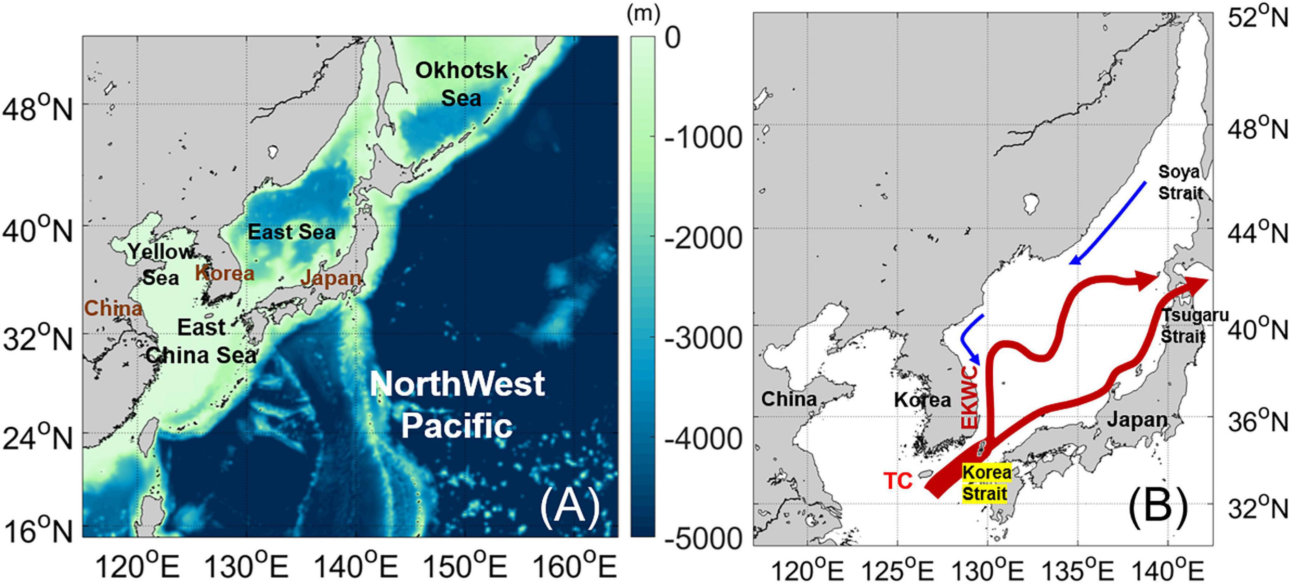
Figure 1. (A) Bottom topography (unit: m) of the NWP in the RCM. (B) Main currents present in the study area: Tsushima Current (TC) and the East Korean Warm Current (EKWC).
The ability of sea-level rise to alter tidal regimes has been well documented (Pickering et al., 2012; Pelling and Green, 2014; Passeri et al., 2015; Idier et al., 2017), potentially intensifying extreme sea levels (Smith et al., 2010; Warner and Tissot, 2012; Arns et al., 2015). The effect of SLR on tidal amplitudes has also been investigated for the NWP marginal seas (Gao et al., 2008; Yan et al., 2010; Pelling et al., 2013; Zhang and Ge, 2013; Kuang et al., 2017), with larger changes observed in shallow coastal regions rather than deeper regions.
We defined practical sea-level rise (PSLR) here as the sum of relative sea-level rise, the change in tidal amplitude and the change in natural variability, as the evaluation of this parameter may help identify localities with more severe SLCs. More detailed future SLC projections can also help with local risk assessments, mitigation, and adaptation planning. In this study, local SLR was simulated according to increasing spatiotemporal resolutions of the downscaled regional model, and with the inclusion of tidal influences for the NWP marginal seas. Downscaled SLCs were projected using regional ocean climate models (RCMs) driven by four different GCMs. The data and model configuration used are introduced in Section 2, comparisons between GCMs and RCMs using historical data are presented in Section 3, the projections of SLCs by GCMs and RCMs under two climate change scenarios are discussed in Section 4, and conclusions are provided in Section 5.
Data and Methods
Global Climate Models
Global climate models driven by observed greenhouse gas concentrations until 2005, and subsequently by intermediate (RCP 4.5) or high-end emissions (RCP 8.5) scenarios from 2006 to 2100, were selected for analysis (Church et al., 2013). All GCM simulations were acquired from the CMIP5 database (Taylor et al., 2012), and 13 of the 48 models available provided all oceanic and atmospheric variables required for deriving boundary values of the RCM.
Following performance evaluations of sea-level and sea surface temperature (SST) predictions based on observations from the NWP, four CMIP5 GCMs were selected for regional downscaling. The spatial mean sea surface heights (SSHs) along the lateral boundaries of the RCM from 1976 to 2005 were compared with reconstructed sea-level data created using cyclostationary empirical orthogonal functions derived from satellite altimetry and sea-level measurements from tidal gauges (Hamlington et al., 2011). Spatial mean SST along the lateral boundary grid was compared with a combination of the climatological mean from the World Ocean Atlas 2009 (WOA09) (Levitus et al., 2010) and anomaly data (Levitus et al., 2012). The corrected SSH (zos_c) was calculated for direct comparison with the reconstructed sea-level data according to Equation (1):
where the SSH above the geoid (zos) is the dynamic sea-level reflecting fluctuations from the geoid (Griffies et al., 2014). The global mean SSH (zos_m) was removed from zos to exclude spurious model drift in each GCM. Global mean SLCs due to thermosteric effects (zostoga), and the correlated change in ocean mass (i.e., mass effect; bary_sle) were then added. Different values for the thermosteric sea-level were used depending on the GCM, and the mass effect on sea-level was calculated as the sum of the contributions from glaciers, ice sheets, and land water storage (Church et al., 2013). For all GCMs, annual mass effects were linearly interpolated to monthly. GCM model performance was evaluated in two ways: The performance index (PI) to evaluate GCMs can be defined according to Equations (2, 3):
where X is the root mean square error (RMSE) of the annual variables, and E is the absolute difference in trends between GCMs and observations. The overall RMSE and trends of SSH between GCMs and the observations were evaluated from the spatial mean along the lateral boundary (PISSH). The RMSE and trends of SSH and SST were also evaluated simultaneously (PISSH&SST). The numbers of selected grids for calculating spatial mean along the lateral boundary were approximately 200 and 800 for the observations and GCMs, respectively.
Performance evaluation results are shown in Table 1. To select the most reasonable number of GCMs for dynamical downscaling, the PIs for each multi-model ensemble (EPI) were ranked by increasing ensemble size. Both EPISSH and EPISSH&SST were best with two ensemble members, as these values increased when ensemble size ≥ 3. Four GCMs were selected for our experiment. The top 2 models, IPSL-CM5A-LR and IPSL-CM5A-MR, were selected based on minimum EPISSH. NorESM1-M and MPI-ESM-LR which showed minimum EPISSH&SST, were also selected. IPSL-CM5A-LR and IPSL-CM5A-MR have a coarser horizontal grid resolution (∼2.0°; Dufresne et al., 2013), whereas NorESM1-M and MPI-ESM-LR have resolutions of ∼1.1° and 1.5°, respectively. Figure 2 shows topography of selected GCMs in the NWP.
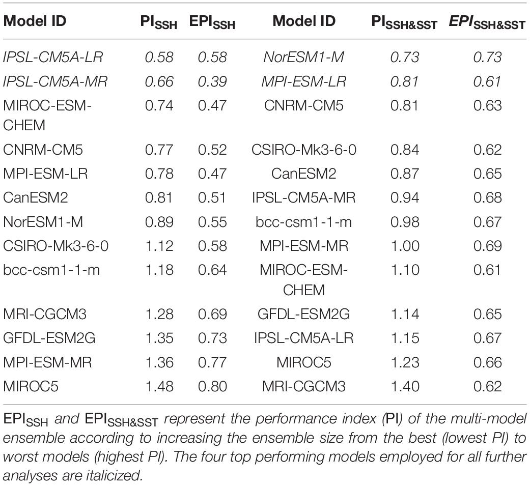
Table 1. GCMs results based on PISSH and PISSH&SST (see Equations 2, 3, respectively).
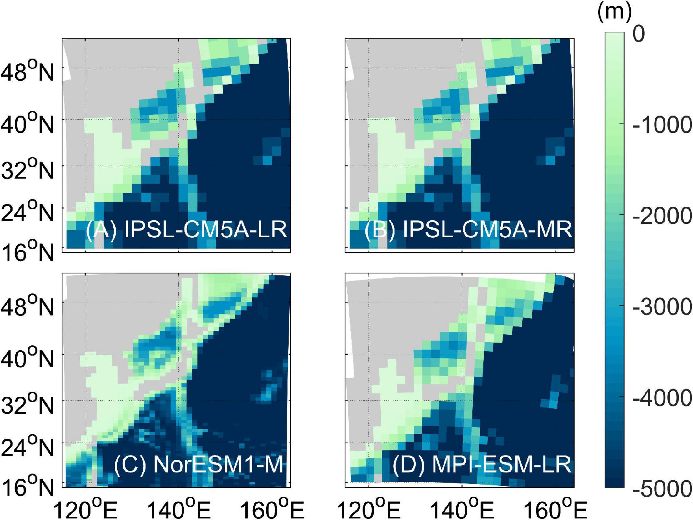
Figure 2. Bottom topography (unit: m) of: (A) IPSL-CM5A-LR (GCM-IPSL-L), (B) IPSL-CM5A-MR (GCM-IPSL-M), (C) NorESM1-M (GCM-Nor), and (D) MPI-ESM-LR (GCM-MPI) with gray land mask.
Regional Ocean Climate Models
The Regional Ocean Modeling System (ROMS) was employed to downscale and project long-term SLCs in the NWP marginal seas (Shchepetkin and McWilliams, 2005). The ROMS has a free-surface and uses a Boussinesq approximation. This model uses the hydrostatic primitive equation, and is discretized based on the Arakawa-C staggered grid in the horizontal direction. The RCM domain (15°–52° N, 115°–164° E) covered the NWP and its marginal seas (Figure 1A), with a horizontal grid size of 1/20°. In the vertical direction, 40 layers were applied according to the scheme of Song and Haidvogel (1994), and resolution varied according to topography, increasing in shallower marginal seas. The employed scheme minimized the pressure gradient error at the slope. The RCM was initialized with temperature and salinity data from the World Ocean Atlas 1998 (WOA98) (Antonov et al., 1998; Boyer et al., 1998), and included a spin-up period of 10 years, beginning with the initial conditions in 1976. Subsequently, the RCMs were continuously simulated from 1976 to 2100.
Daily mean atmospheric surface variables of GCMs, such as mean sea-level pressure, 10-m wind, 2-m air temperature, specific humidity, and shortwave radiation were used for surface forcing. A bulk formula was employed to calculate surface heat flux (Fairall et al., 2003), and monthly GCM temperature, salinity, sea-level, and velocities were applied to the ocean lateral boundary in the RCMs. Chapman conditions were adopted for the sea-level (Chapman, 1985), Flather radiation conditions for barotropic velocities (Flather, 1976), and clamped (Dirichlet) conditions for baroclinic velocities, ocean temperature, and salinity. Chapman and Flather conditions allow surface gravity waves generated within the model domain to propagate out through the open boundary with minimal impedance or reflection, while simultaneously imposing tidal sea-levels and currents from the GCMs to the RCMs (Solano et al., 2020). Clamped conditions were applied for all other variables to directly reflect the oceanic forcing of GCMs. All monthly variables were linearly interpolated at every model time step, and applied to the lateral boundaries. RCM sea-levels increased over time to mimic the SLR at the lateral boundary by incorporating the corrected SSH (zos_c).
Tides were included at the oceanic lateral boundary using 10 tidal components (M2, S2, N2, K2, K1, O1, P1, Q1, Mf, Mm) provided by the TPXO7 ocean tide model (Egbert and Erofeeva, 2002). Tidal amplitudes and phases at the boundary were assumed to be constant for historical simulations and future projections, as changes in the tides caused by SLR are comparatively small along the boundary of the RCM in the open ocean (Pickering et al., 2017). Monthly freshwater discharge data from the Yangtze was used for historical simulations. The mean discharge across the historical period for each river was used for future projections. We used the climate monthly mean data from the Global River Discharge Database (Vörösmarty et al., 1996) for eleven other rivers around the Yellow Sea (YS) and Bohai Sea for both historical simulation and future projection. Topography data were obtained from the Earth Topography 1 arc minute (ETOPO1) dataset and interpolated into the RCM grid points (Amante and Eakins, 2009).
For clarity, the simulations of IPSL-CM5A-LR, IPSL-CM5A-MR, NorESM1-M, and MPI-ESM-LR are hereafter referred to as GCM-IPSL-L, GCM-IPSL-M, GCM-Nor, and GCM-MPI, respectively; whereas the respective downscaled simulations from the RCM are referred to as RCM-IPSL-L, RCM-IPSL-M, RCM-Nor, and RCM-MPI.
Historical Simulations
Surface Temperature
Sea surface temperature is a fundamental indicator of climate change and has a significant correlation with thermal expansion and steric SLC (Casey and Adamec, 2002). Accordingly, SST has increased in the NWP as well (Levitus et al., 2000). GCM and RCM SSTs were compared with averaged satellite observations averaged from 1982 to 2005 (Figure 3). The optimum interpolation sea surface temperature (OISST), which uses satellite SST data from the Advanced Very High-Resolution Radiometer (Reynolds et al., 2007), was employed to compare with model simulations. Figure 3A shows the satellite-based SST observations for the NWP marginal seas. The Kuroshio supplies warm water (>20°C) to the East China Sea (ECS). The Tsushima Current (TC), through the Korea Strait, separates into the nearshore branch along the Japanese coast and the East Korean Warm Current (EKWC) along the Korean coast. Surface temperatures > 15°C in the East/Japan Sea (EJS) were defined as the path of the TC and EKWC. The warm EKWC flows northward as a western boundary current along the Korean coast and separates from the coast at 37 ∼ 38° N. Surface temperatures in the EJS where the TC and EKWC supply heat is notably higher than the YS at the same latitude.
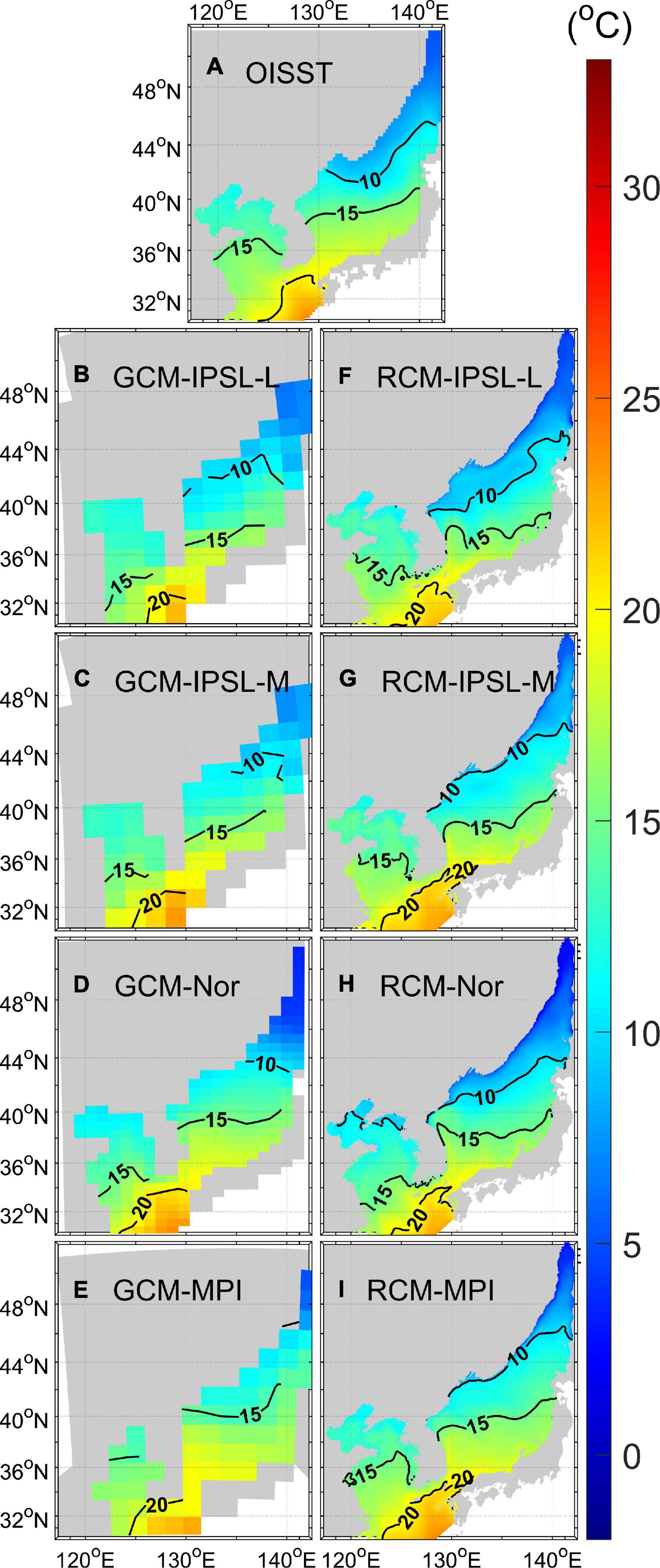
Figure 3. Mean SSTs (units: °C) in the NWP marginal seas: (A) SST from OISST satellite observations, (B–E) GCMs, and (F–I) RCMs, 1982–2005.
Latitudes of the 15 °C isotherms showed a large difference among the GCMs, but were more similar among the RCMs. The SSTs of GCM-IPSL-L and GCM-IPSL-M were underestimated in the TC and EKWC paths. The absence of the EKWC decreases the SST. The latitudes of the 10 °C isotherm in the EJS showed a large difference between both the GCMs and RCMs. The GCMs expressed spatial SST patterns correlating to different surface atmospheric forcing, whereas the 10°C isotherm latitudes in the RCMs were similar despite employing the different surface atmospheric forcing variables. The RMSE was improved in RCM-Nor and RCM-MPI because of a considerable improvement in the warm bias of the northern EJS. The average RMSE of the RCM in the EJS was 0.26°C lower than that of the GCM (Table 2). Further, only RCM-IPSL-L and RCM-Nor showed improvements in modeling the YS and ECS (YS-ECS), where spatial SST differences were relatively small (Table 2).
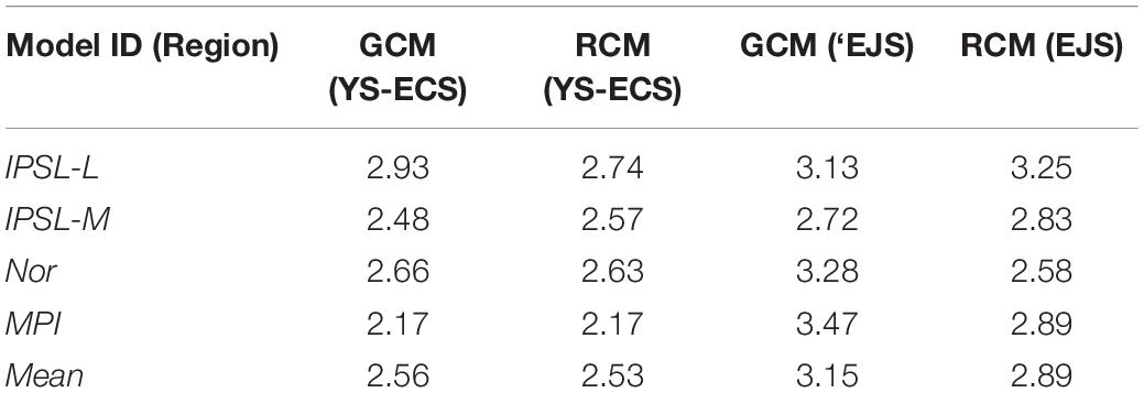
Table 2. The root mean square error (RMSE; units: °C) between the satellite-derived SST and modeled SST in the shallow (YS-ECS) and deep seas (EJS).
Surface Current
Dynamic sea-levels are closely related to oceanic currents (Couldrey et al., 2021); thus, the surface currents of GCMs and RCMs were compared with satellite-derived surface geostrophic currents averaged across 1993–2005 (Figure 4). The geostrophic currents calculated using altimeter data from the Copernicus Marine Environment Monitoring Service (CMEMS) were used for comparison. Figure 4A shows the satellite-derived currents in the NWP marginal seas, and pattern correlation coefficients (PCCs) were calculated for the geostrophic velocities in the YS and ECS (Supplementary Table 1). GCM-Nor (Figure 4D) most closely resembled the observed coastal currents, while GCM-IPSL-L (Figure 4B) and GCM-IPSL-M (Figure 4C) performed worse. All RCMs yielded improved PCCs, especially in RCM-IPSL-L and RCM-IPSL-M, where the mean value across all RCMs (0.49) was 0.30 greater than that of GCMs (0.19).
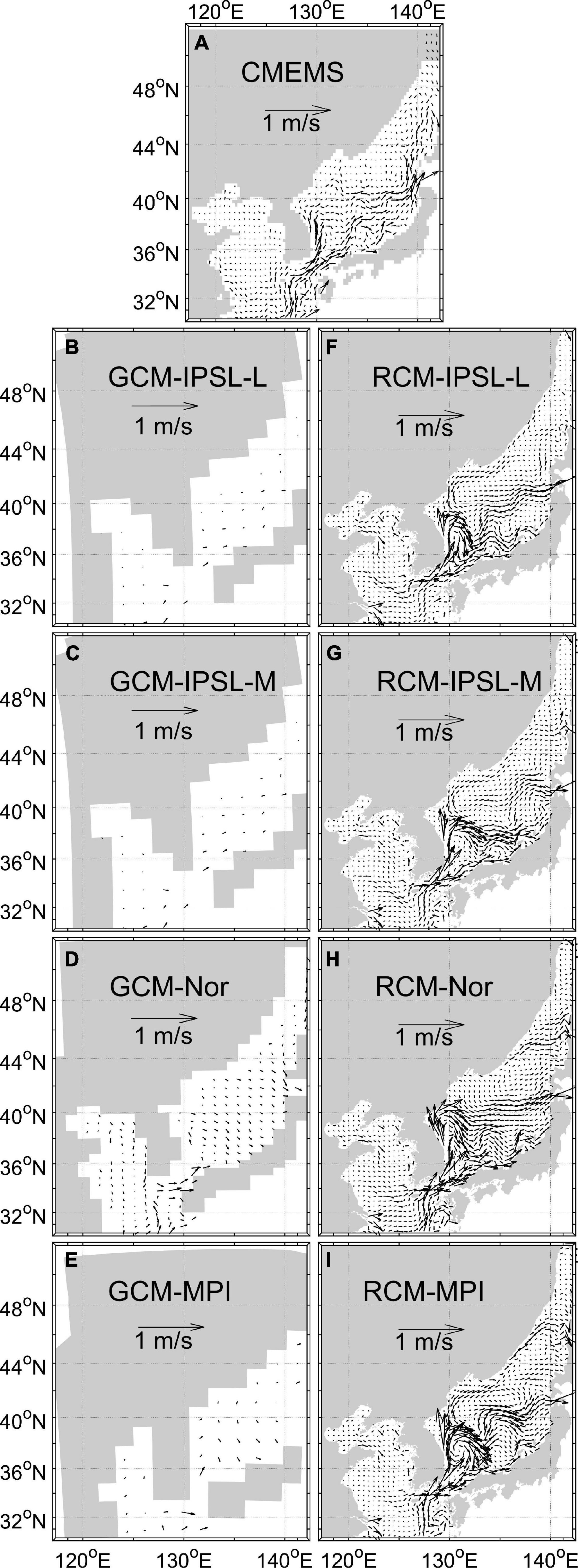
Figure 4. Mean surface currents in the NWP marginal seas: (A) Satellite-derived geostrophic current from CMEMS, and mean surface currents of panels (B–E) GCMs and (F–I) RCMs, 1993–2005.
GCM-IPSL-L and GCM-IPSL-M, which have the coarser resolutions, did not effectively resolve the TC and EKWC (Hogan and Hurlburt, 2000) in the EJS, whereas the RCMs were able to simulate the paths of these currents distinctly. The PCCs in the EJS supported a distinct difference between the GCMs and RCMs (Supplementary Table 2). GCM-IPSL-L and GCM-IPSL-M showed negative PCCs of northward velocities, as they were unable to simulate the currents’ detailed structure (including the EKWC in the EJS). Conversely, the PCCs of RCM-IPSL-L and RCM-IPSL-M increased by 0.26 and 0.31, respectively. Specifically, the RCMs simulated the northeastward TC along the Japanese coast and the northward EKWC along the Korean coast (Figures 4F–I). However, the separation latitudes of the EKWC varied among the RCMs. RCM-Nor shows the northernmost separation latitude among the RCMs because of the overshooting EKWC (Figure 4H).
Sea Surface Height
The SSHs from each model simulation were compared with satellite-derived observations provided by the CMEMS (Figure 5). The observational SSH products computed using sea-level anomaly and mean dynamic topography data were averaged for 1993–2005, and the modeled SSH values were similarly averaged across the same period. Sea-level observations were higher in the southeastern area where the Kuroshio passes and lower in the YS (Figure 5A). All RCMs had high PCCs (0.97) with the CMEMS for horizontal sea-level distributions in the YS-ECS (Supplementary Table 3), whereas the mean PCC of the GCMs (0.88) was lower. The PCC of GCM-MPI was the lowest due to the high sea-level in the YS (Figure 5E). The oversimplified topography of the GCM-MPI (Figure 2D), which fails to resolve the Taiwan Strait and allocates a single cell to the Korea Strait, may be causing a weak circulation and high sea-level in the YS-ECS, as these estimates were improved with the more accurate topographic conditions of the RCMs.
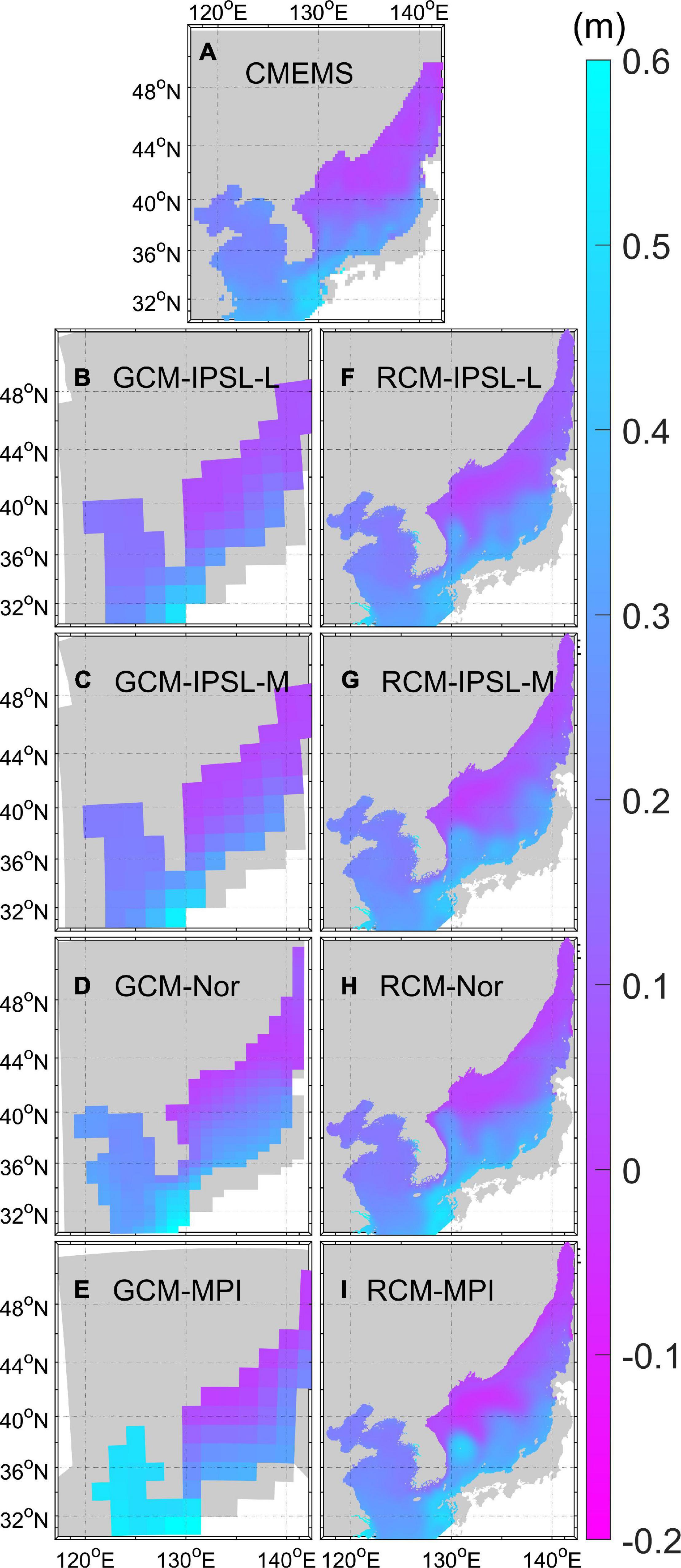
Figure 5. Horizontal distribution of the mean sea-level (unit: m) in the NWP marginal seas: (A) Mean sea-level calculated from CMEMS absolute dynamic topography, and those of the (B–E) GCMs and (F–I) RCMs, 1993–2005.
Satellite-derived SSHs in the EJS were higher in the southern warm waters along the paths of the TC and EKWC, and lower in the northern cold-waters (Figure 5A). GCM-IPSL-L and GCM-IPSL-M showed similar SSH distributions, and could not resolve the higher SSHs in the EKWC path (Figures 5B,C), resulting in relatively low PCCs of 0.76 and 0.85 in the EJS, respectively (Supplementary Table 3). Conversely, all RCMs captured the high SSHs in the path of the EKWC (Figures 5F–I), yielding slightly improved PCCs over GCMs. RCM-Nor maintained the best performance in the EJS (0.93), whereas RCM-IPSL-M and RCM-MPI PCCs (0.82 and 0.80) were slightly lower than GCM-IPSL-M and GCM-MPI (0.85 and 0.92). The low PCCs of two RCMs occur in the northern EJS.
Comparisons of sea-level variability between the model and the observation highlighted the differences between the GCMs and RCMs (Figure 6). Interannual sea-level variability was defined here as the standard deviation after annual signals and linear trends from 1993 to 2005 had been removed. Satellite-derived SSHs showed large variations (>5 cm) in the warm water region of the EJS likely due to the strong currents and active eddy motions, whereas weak variations (<2 cm) were observed in the northern cold-water region. The calculated variabilities in the YS-ECS were between 1 and 5 cm. Further, only the RCMs were able to resolve the spatial differences in the variability of the EJS. The satellite-based sea-level variation in the EKWC (near 38° N, 131° E) was 5.47 cm, notably more similar to those recorded in the RCMs (5.78 cm) compared to the GCMs (2.00 cm).
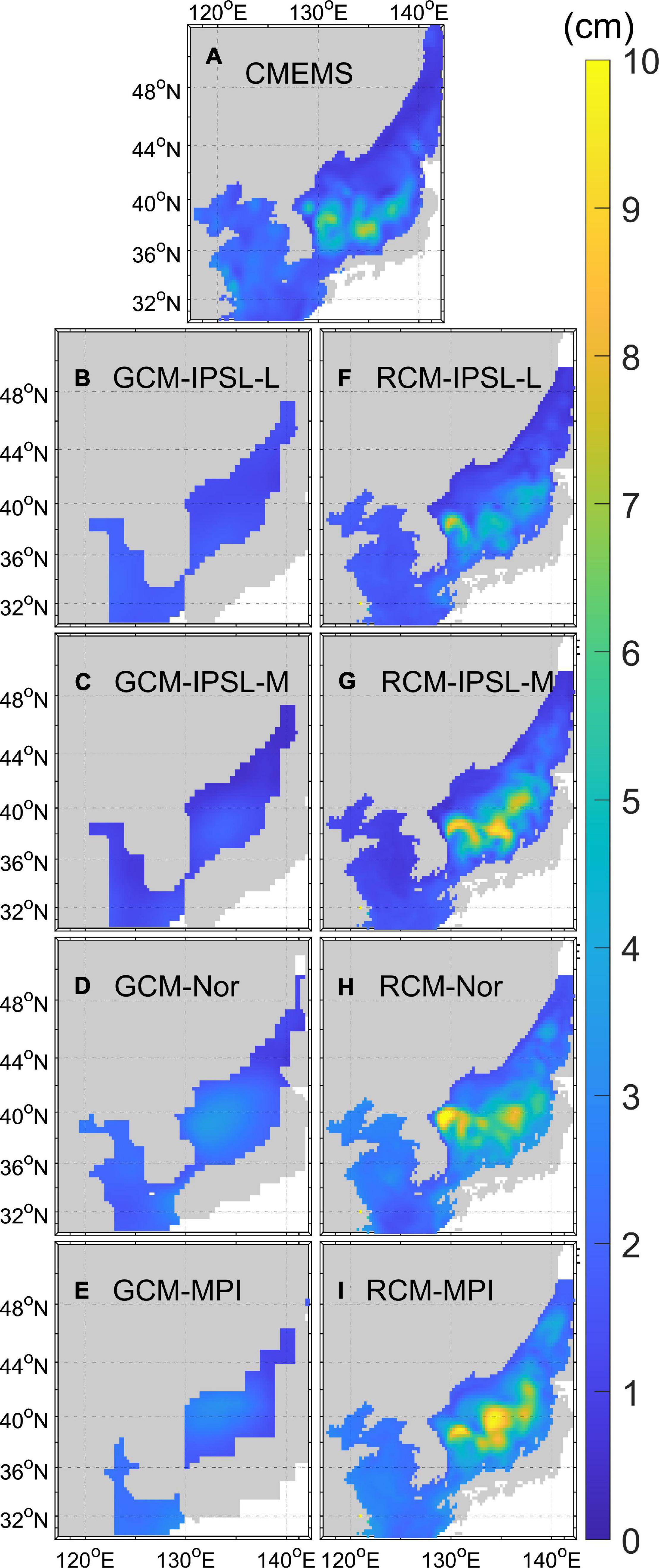
Figure 6. Horizontal distribution of the standard deviations (unit: cm) for mean annual sea-level anomalies after removing linear trends, from: (A) CMEMS, (B–E) GCMs, and (F–I) RCMs, 1993–2005.
To validate the tidal simulations, the sums of the modeled amplitudes for four major tidal components (M2, S2, O1, and K1) were compared between the RCMs and the observations at 14 selected points along the YS (Choi, 1980), in addition to 5 tidal stations operated by the Korea Hydrographic and Oceanographic Administration (KHOA) in the EJS. The observed sum of the tidal amplitudes was large (>3 m) along the Korean coast in the YS, but only < 0.5 m in the EJS (Figure 7A). The spatial distribution of the simulated tidal amplitudes in 2005 was comparable to the observations, yielding correlation coefficients of 0.97 for all RCMs (Figure 7B), with an average absolute error of 0.15 m.
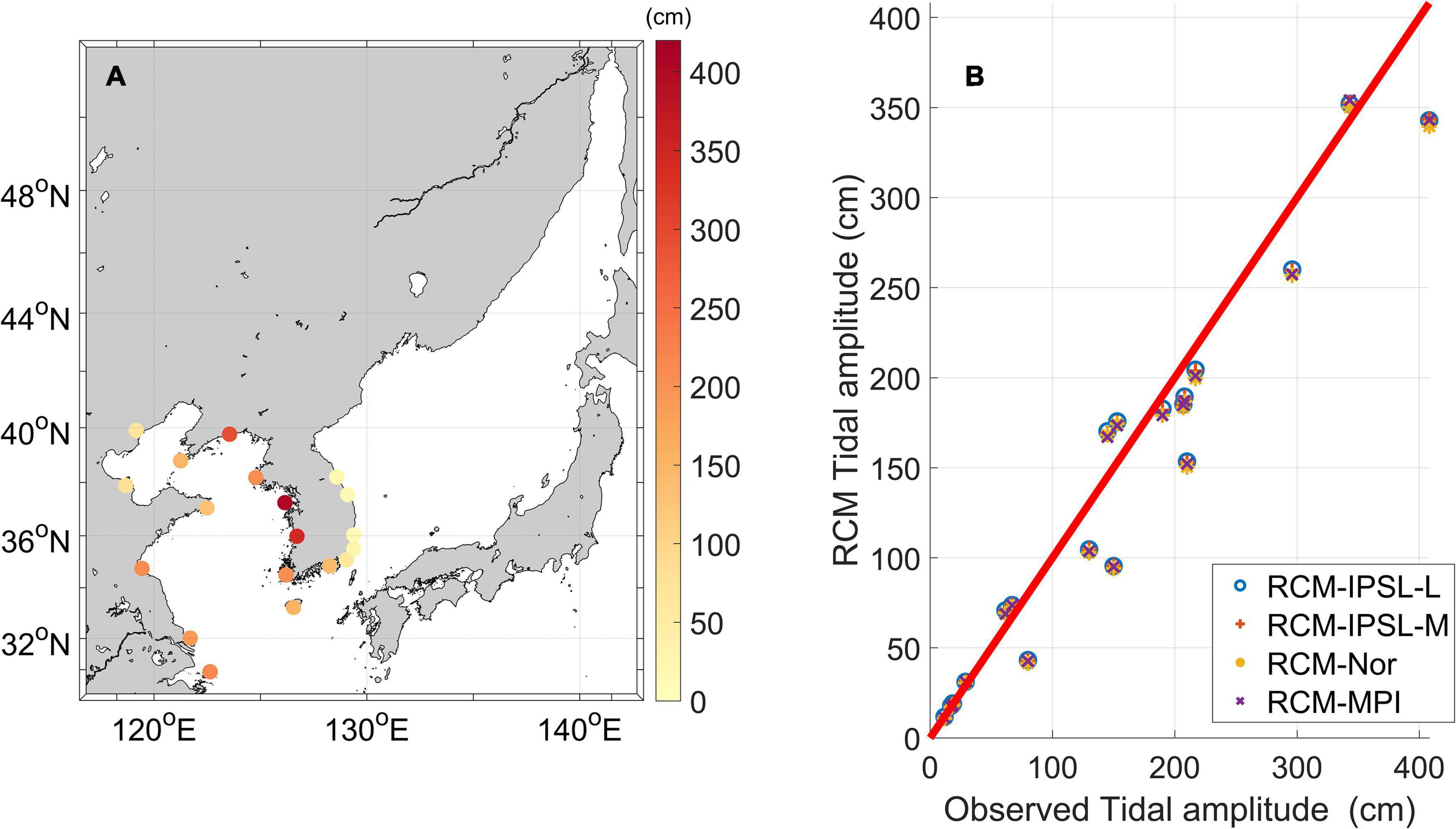
Figure 7. (A) Sum of the amplitudes (unit: cm) for four major tidal constituents (M2,S2,K1,andO1) at the observation station from Choi (1980). Point colors represent the tidal amplitude at the station. (B) Comparison of observed and 2005 RCM tidal amplitudes.
Projections for the 21St Century
Projection of Sea-Level Changes
Timeseries of the mean annual data showed the projected SLR according to the warming signal under future climate scenarios for both the GCMs and RCMs (Figure 8). The data represent the spatial means of the NWP marginal seas (Figure 1B). In addition to the gradual increase due to the warming signal, annual mean sea-level also showed the interannual variation due to the internal natural variability and external variation from the lateral boundary sea-level. The mean correlation coefficient values between the sea-levels of GCMs and RCMs in the NWP were both 0.99 under RCP 4.5 and 8.5 scenarios, respectively. The direct response of RCMs to the sea-level change of GCMs forced at the lateral boundary might result in this high correlation. The ensemble mean SLR estimates of the RCMs from 2081–2100 relative to that in 1976–2005 for RCP 4.5 and 8.5 scenarios in the NWP marginal seas were 46 and 65 cm, respectively. The ensemble spreads of annual sea-levels among the GCMs were 4.3 and 4.5 cm under RCP 4.5 and RCP 8.5 scenarios, respectively, whereas those of the RCMs were 2.6 under both scenarios.
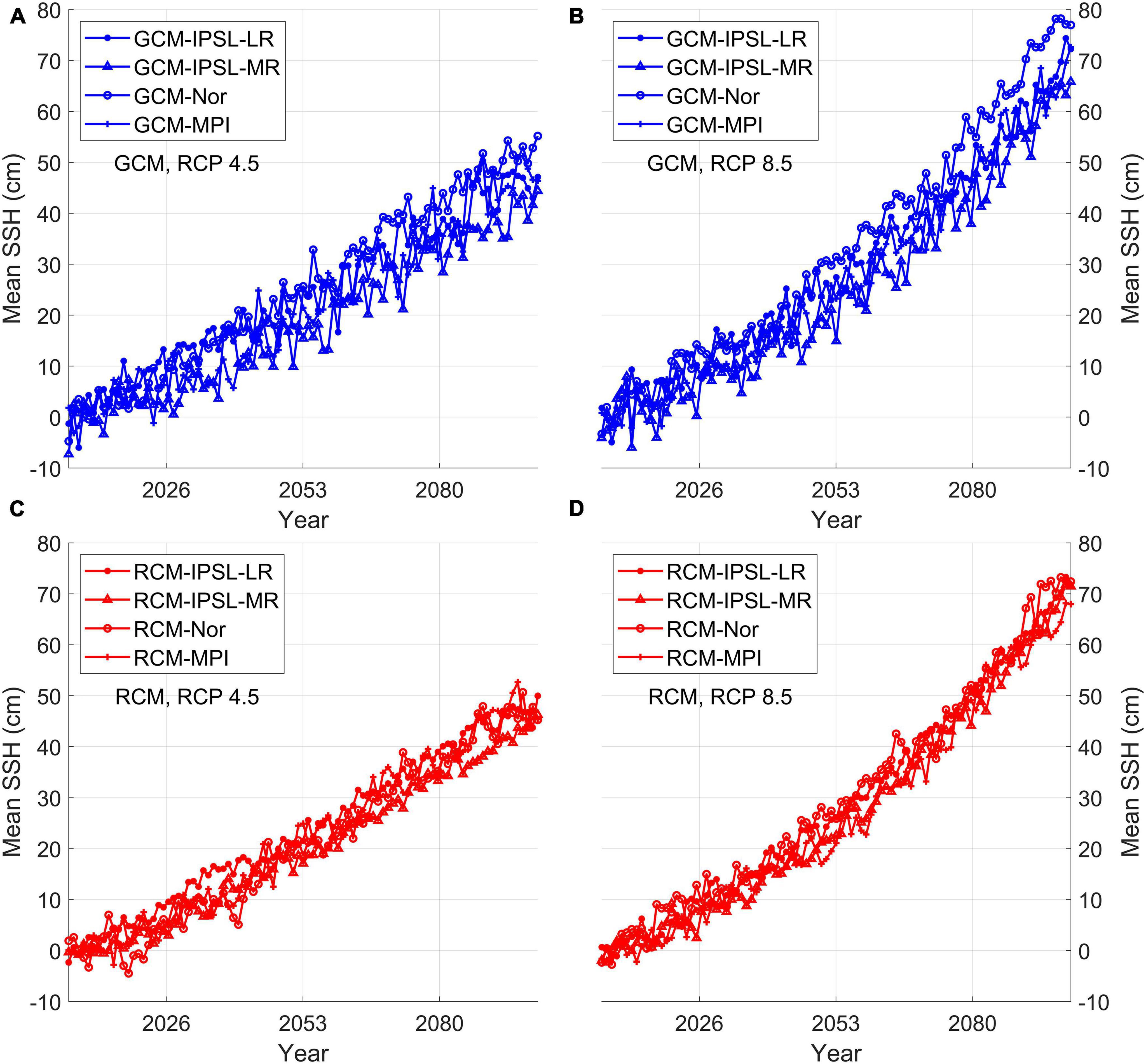
Figure 8. Timeseries of sea-level changes (unit: cm) from 2006 to 2100, for two representative concentration pathway (RCP) scenarios: (A) GCMs—RCP 4.5, (B) GCMs—RCP 8.5, (C) RCMs—RCP 4.5, and (D) RCMs—RCP 8.5.
Figure 9 shows the projected mean SLR between 1986–2005 and 2081–2100. The coarse resolution GCMs could not simulate SLR near the coastal area, and the mean SLR for the highest (GCM-Nor) and lowest models (RCM-IPSL-M) were 53.3 cm and 41.4 cm, respectively (Table 3). The RCMs showed relatively high SLR in the paths of the EKWC (near 38°N, 131°E) and TC (near 42°N, 138°E) where non-seasonal variations of the SSH are predominant (Choi et al., 2004). The maximum spatial differences in the SLR of the EJS were 5.5, 4.4, 2.0, and 9.6 cm for GCM-IPSL-L, GCM-IPSL-M, GCM-Nor, and GCM-MPI, respectively, whereas those for RCM-IPSL-LR, RCM-IPSL-MR, RCM-Nor, and RCM-MPI were 29.1, 17.8, 39.6, and 31.4 cm, respectively. Further, these spatial differences in SLR were three times higher than the maximum natural variability observed throughout the historical period (Figure 6). High SLR in the EJS is related to sea-level variations caused by the north-south migration of the polar front, meandering of the EKWC and TC, and active motions of the semi-permanent Ulleung Warm Eddy (Choi et al., 2004; Hogan and Hurlburt, 2006), none of which could be resolved in the coarse resolution GCMs.
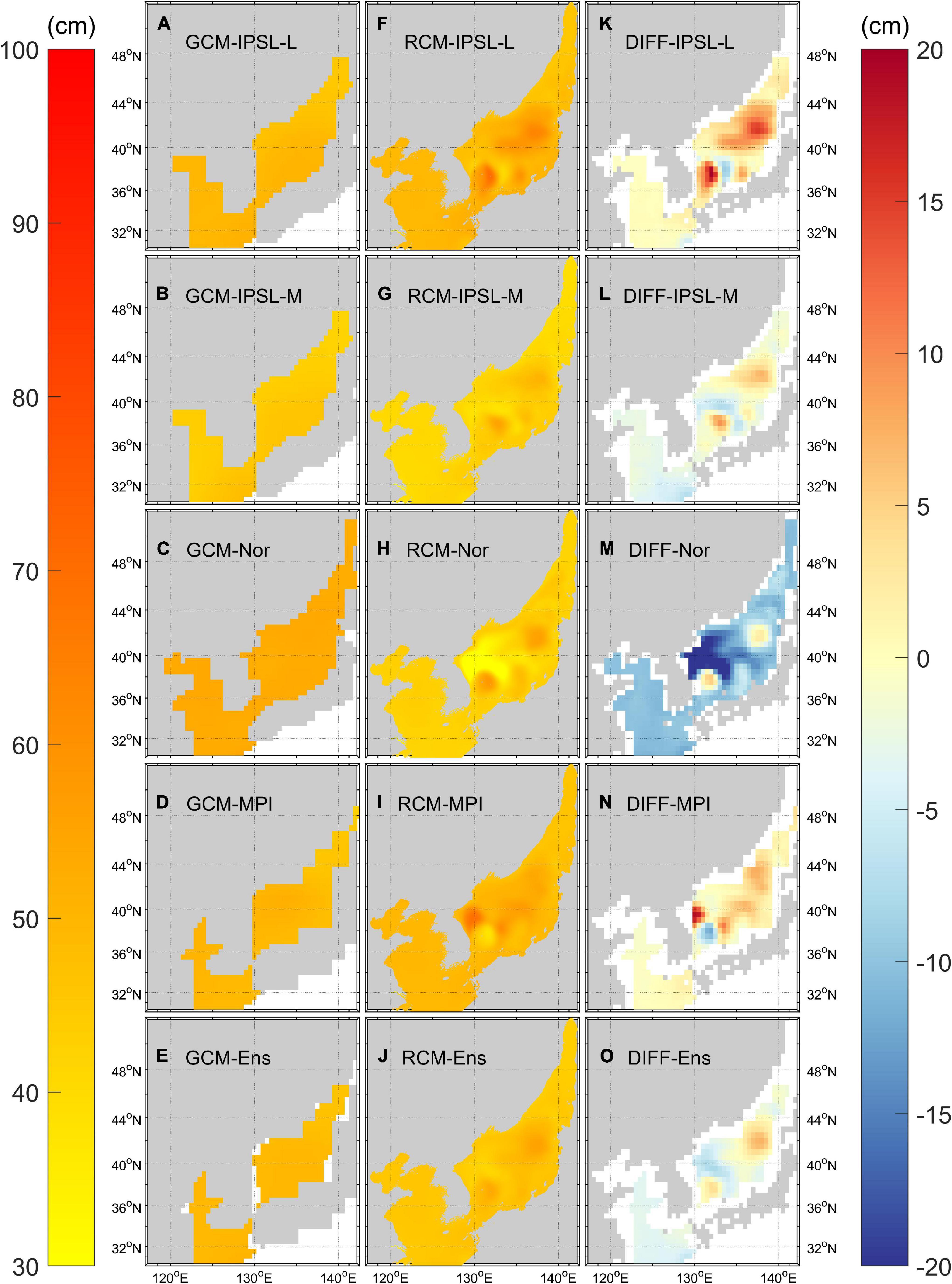
Figure 9. Sea-level rise (unit: cm) between 1986–2005 and 2081–2100 in the NWP marginal seas under RCP 4.5 scenario according to panels (A–D) GCMs, and (F–I) RCMs. (E) and (J) represent the ensemble means of the GCMs and RCMs, respectively. Differences between the two modeling methods (RCM-GCM) are shown in panels (K–O).
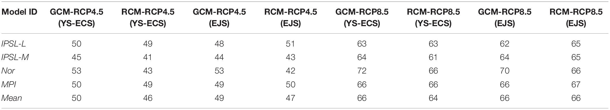
Table 3. Sea-level rise (SLR; unit: cm) of GCMs and RCMs between 1986–2005 and 2081–2100 (Figures 9, 10) in the shallow (YS-ECS) and deep seas (EJS), under RCP 4.5 and RCP 8.5 scenarios.
We calculated the local steric SLC (Supplementary Figure 1) following Griffies et al. (2016), and subsequently the manometric SLCs (Supplementary Figure 2) by subtracting steric SLC from SLR. The steric SLCs were high in the deep regions, and lower in the shallow locations. However, the inverse patterns were observed for manometric SLC. These dependences of the local steric and manometric SLC patterns on water depth are consistent with those reported in the Northwestern European shelf seas (Hermans et al., 2020). The mean steric SLC differences between GCMs and RCMs were 4.19 and 15.00 cm in the YS-ECS and EJS, respectively.
The projected SLRs under RCP 8.5 were predictably higher than those under RCP 4.5 (Figure 10), reaching its maximum in GCM-Nor (71.6 cm), and minimum in GCM-IPSL-L (63.3 cm) for the YS-ECS (Table 3). Higher levels of SLR appeared along the EKWC and TC paths as in RCP 4.5 scenario models. The spatial differences in SLR for the EJS ranged from 5.9 to 13.9 cm (GCM-Nor–GCM-MPI). The differences between RCMs were larger than that of GCMs (39.3, 24.1, 34.4, and 38.4 cm for RCM-IPSL-LR, RCM-IPSL-MR, RCM-Nor, and RCM-MPI, respectively).
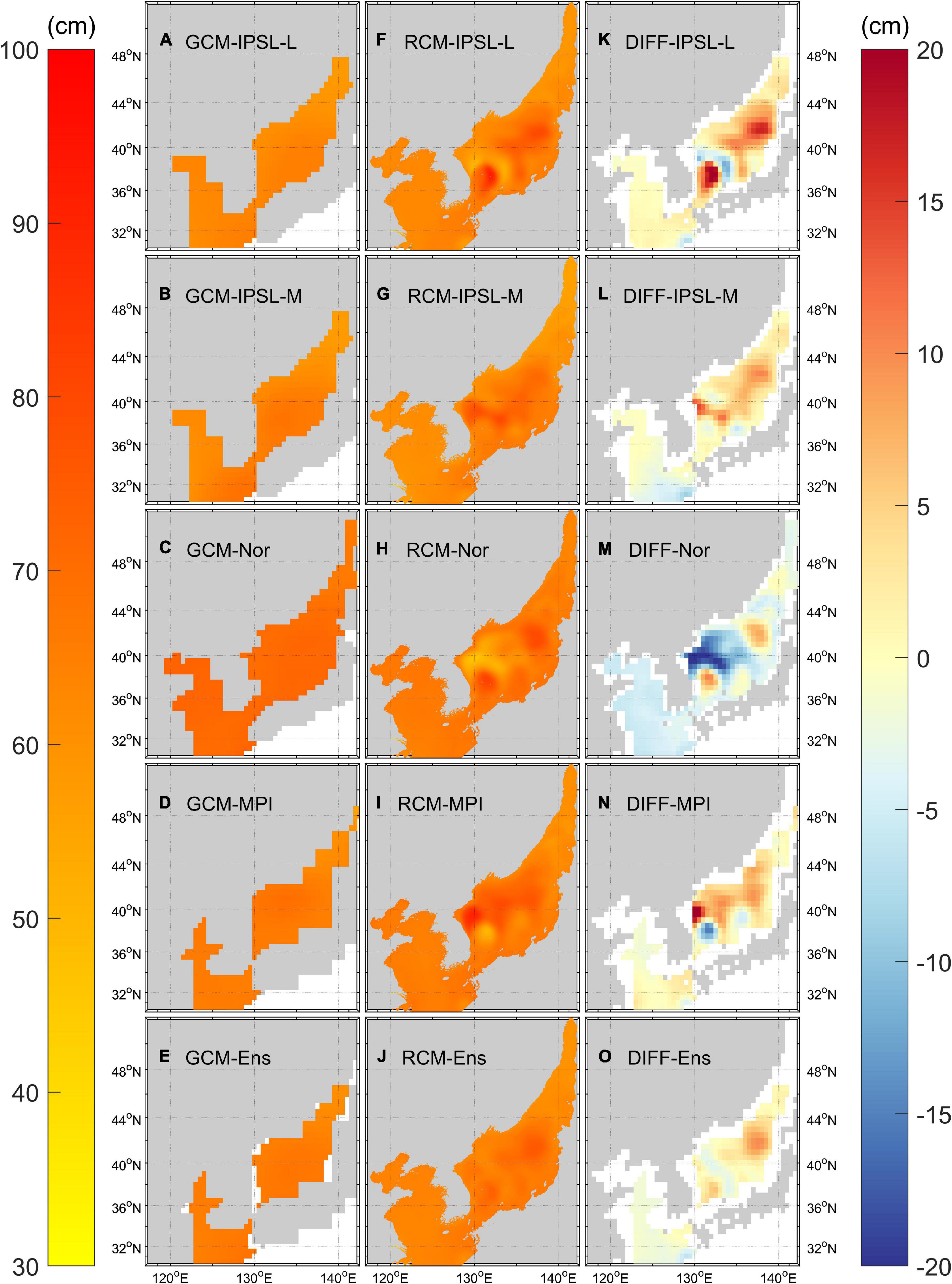
Figure 10. Sea-level rise (unit: cm) between 1986–2005 and 2081–2100 in the NWP marginal seas under RCP 8.5 scenario according to panels (A–D) GCMs, and (F–I) RCMs. (E) and (J) represent the ensemble means of the GCMs and RCMs, respectively. Differences between the two modeling methods (RCM-GCM) are shown in panels (K–O).
Under RCP 8.5, steric (Supplementary Figure 3) and manometric SLC (Supplementary Figure 4) followed water depth (like RCP 4.5). The mean steric SLC difference between the GCMs and RCMs was 4.48 and 16.26 cm in the YS-ECS and EJS, respectively. RCM-Nor showed a slightly higher steric sea-level among the RCMs because of the smaller predicted temperature changes than other models in either RCP scenario.
Changes in Tidal Amplitude
The changes in the sum of the tidal amplitudes between 2006 and 2100 under RCP 4.5 and RCP 8.5 scenarios are shown in Figure 11. Four major constituents (M2, S2, K1, and O1) were selected for summation, revealing that the tidal amplitude increase in the shallow region was > 5 cm under RCP 4.5, and > 10 cm under RCP 8.5, comparable to the findings of Kuang et al. (2017) in the YS. Although the changes for all RCMs (Supplementary Figure 5) were calculated, only the ensemble mean in Figure 11 is presented here, due to the overall similarity between the models. The horizontal mean standard deviations among the RCMs were 0.21 and 0.14 cm under RCP 4.5 and RCP 8.5 scenarios, respectively. The different tidal amplitude changes within the same scenario may result from the differences in SLR among the RCMs, as the increase of tidal amplitude was roughly proportional to the SLR. SLR increases tidal wave speed, leading to the movement of amphidromic points. However, the shift of these points is not a simple function of SLR, as its movement is two-dimensional, and the curvature of corange lines creates a complex response (Pickering et al., 2017). Thus, changes in tidal amplitude were not simply proportional to the SLR in the YS (Feng et al., 2015).
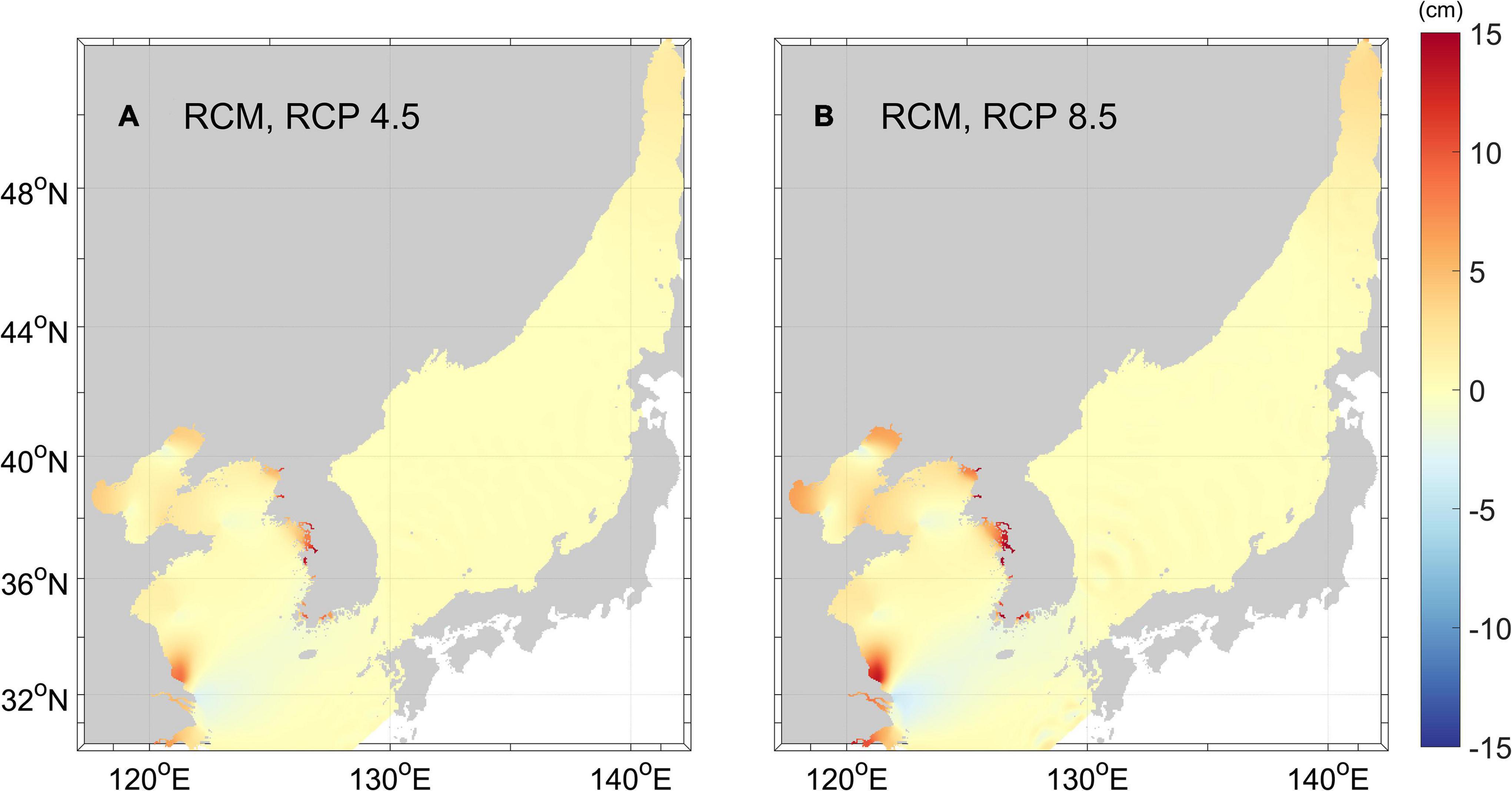
Figure 11. Changes in the sum of the mean ensemble tidal amplitudes (unit: cm) for four major tidal constituents (M2,S2,K1,andO1) of the RCMs between 2006 and 2100, for: (A) RCP 4.5, and (B) RCP 8.5 scenarios.
As tides are shallow-water ocean waves, tidal wave speed (c) can be approximated by Equation (4) if bottom friction is neglected:
where g is gravitational acceleration, and H is water depth. As tidal wave speed is positively correlated with depth, increasing sea-levels will cause tidal waves to propagate more quickly. At that time, wavelength (λ=c×T) also increases with SLR, and displacement of the amphidromic point due to the increase in wavelength significantly affects tidal amplitude (Kuang et al., 2017), and thus the redistribution of tidal energy (Song et al., 2013; Feng et al., 2019).
The tidal amplitude changes for each major constituent (M2, S2, K1, or O1) are presented in Supplementary Figures 6–9. Amplitude changes were more remarkable in shallower waters under both RCP 4.5 and RCP 8.5 scenarios. Tidal amplitude changes in this study showed different patterns between diurnal and semidiurnal tidal constituents, expressing large differences in period and wavelength consistent with previous study in the YS (Feng et al., 2019).
Practical Sea-Level Rise
The projections indicated SLR under future climate scenarios. However, the PSLR may differ due to spatially non-uniform changes in natural variability and tidal amplitude. Accordingly, the estimation of PSLR may be beneficial and help inform local risk assessments of climate change.
Practical sea-level rise is defined as according to Equation (5):
where atide is the tidal amplitude change (Supplementary Figure 5), and δ(σSSH) is the difference in natural sea-level variability between the future and the past [2081–2100 (minus) 1986–2005] after removing trends which are linear in the historical period and exponential in RCP scenarios (Supplementary Figure 10). The natural variability is represented by the standard deviation of annual mean sea-level anomalies during each period, and shows large changes (>5 cm) in the EKWC path. Mean spatial natural variability under RCP 8.5 was 1.14 cm greater than that during the historical period.
Although all calculated changes in the PSLR for all RCMs can be seen in Supplementary Figure 11, the ensemble mean is presented in Figure 12. Under RCP 8.5 (RCP 4.5), the PSLR was 66 (47) cm for the YS-ECS. Notably, PSLR reached its maximum in the Jiangsu coastal area [82 (58)] cm and the Gyeonggi Bays [83 (58)] cm near 32.8° N, 121.2° E and 37.3°N, 126.5°E, respectively, due to the increase in tidal amplitude. Furthermore, the PSLR was approximately 21 (13) cm higher than SLR in both regions. Other shallow regions with substantial tidal amplitude changes also displayed higher PSLR values than the surrounding areas.
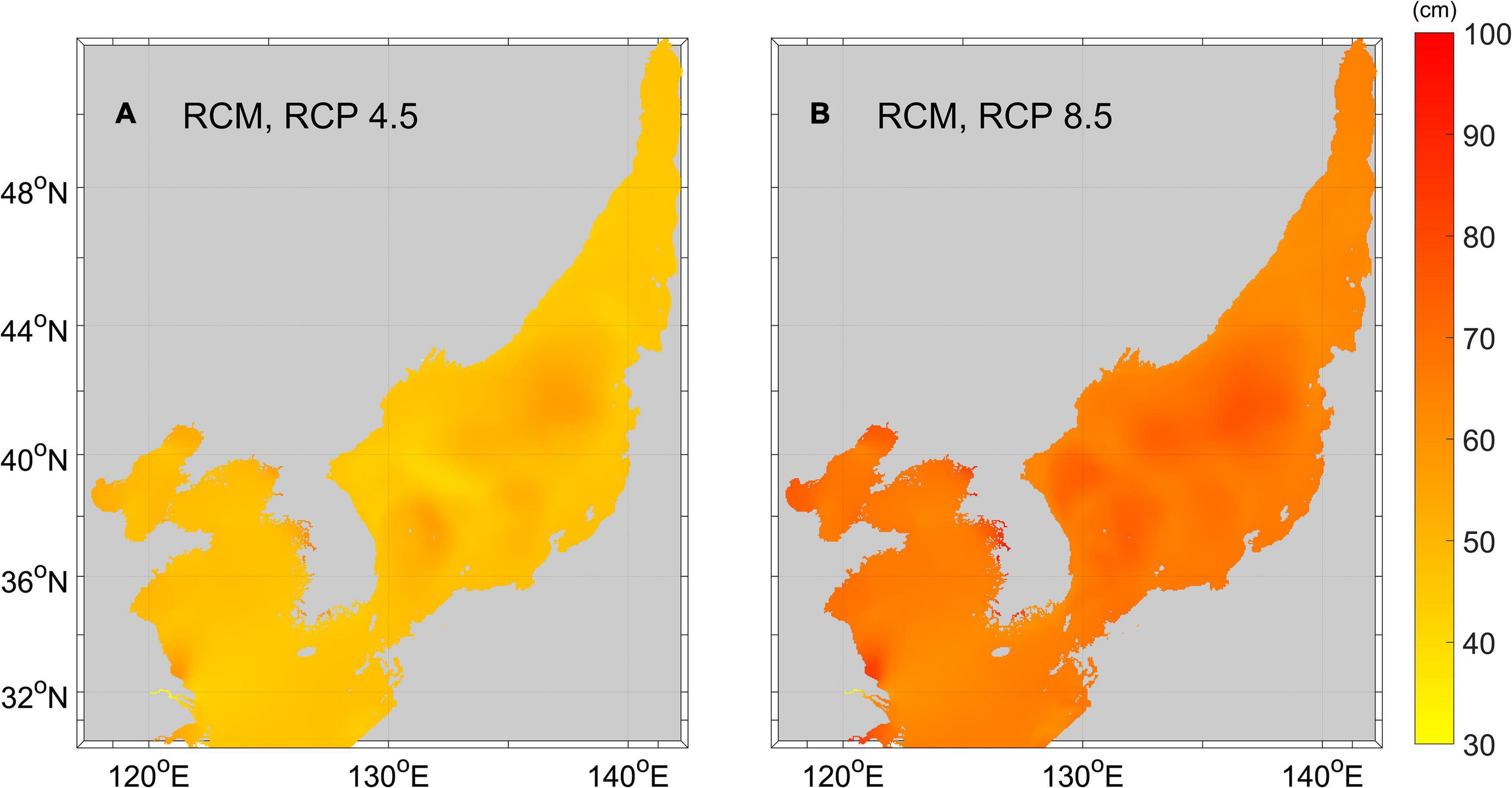
Figure 12. Horizontal distributions of the practical sea-level rise (PSLR; unit: cm) for the RCMs between 1986–2005 and 2081–2100, under: (A) RCP 4.5 and (B) RCP 8.5 scenarios.
The PSLR of the EJS was 67 (47) cm under RCP 8.5 (RCP 4.5) scenario, and the contributions of the natural sea-level variability changes in the EJS were higher than that in the YS-ECS, whereas tidal contributions were higher in the latter seas. The PSLR was 73 (46) cm near the EKWC path (near 39°N, 130°E), ∼5 (2) cm higher than SLR in the same region.
Conclusion and Discussion
In this study, we projected the SLR including barystatic and sterodynamic components considered in lateral boundary sea-level. The projected SLR and local PSLR in the NWP marginal seas were evaluated under intermediate and high-end climate change scenarios using dynamically downscaled RCMs. Climate change signals of the GCMs were directly applied at the lateral model boundaries, and the results showed significant predictive improvements in SST, currents, and SSH compared with coarser resolution GCMs. The high-resolution RCMs used in this study were able to resolve detailed currents and simulated PSLR, having considered changes in sea-level variability and tidal amplitude under two RCP scenarios.
The higher-resolution RCMs could resolve SLCs driven by eddy motions, capturing greater SLR in the EKWC and TC paths of the EJS resulting from strong currents and active eddy motions, whereas the GCMs maintained a limited ability to simulate spatially non-uniform SLR due to their coarse resolution. The RCMs also showed higher steric SLR in the deeper regions of the EJS, supporting the importance of resolving topographic features in SLR projections, as in other downscaled SLR projections (Hermans et al., 2020).
Tidal changes resulting from climate change were also examined using the RCMs, showing an increase in the tidal amplitude by > 15 cm in the shallow region of the YS, consistent with the results of Kuang et al. (2017). Moreover, tidal amplitude changes caused by different SLR values were simulated depending on the RCMs, where previous studies had assumed arbitrary SLR at the open boundary (Kuang et al., 2017; Feng et al., 2019; Jiang et al., 2021). The results suggested that the climate-induced changes in tidal amplitude conventionally missed by GCMs should be considered when estimating extreme sea levels for future coastal flood risk assessments in the marginal seas which is dominated by tides. Flood risks may increase due to the mean SLR, in addition to changes in the magnitude of extreme events, such as tides. Extreme sea level is also affected by storm surges, waves, and a combination of these processes (van de Wal et al., 2019). Besides that, the vertical ground motion may affect the local relative sea-level rise (Raucoules et al., 2013; Palanisamy Vadivel et al., 2021).
Practical sea-level rise, which is defined by the sum of the SLR, tidal amplitude changes, and natural variability changes, was proposed here to estimate the effective SLR. The PSLR suggested that the coastal areas where the tidal amplitude changes were largest in the YS-ECS were likely to be more vulnerable to the effects of SLR due to climate change under RCP scenarios. Dynamical downscaling was important for PSLR simulation in the NWP marginal seas containing a narrow strait, complex coastlines, and are affected primarily by tidal forcing. Most GCMs were unable to consider tidal forcing, and simulated low sea-level variability due to the limitations of capturing active eddy motions. Thus, GCM accuracy was limited when calculating PSLR in the NWP marginal seas. The RCMs resolved eddies, but may be limited in simulating the exact paths of the EKWC. Hogan and Hurlburt (2000) suggested a 1/16° resolution for the improved simulation of the EKWC path, and a 1/32° resolution for an accurate simulation of baroclinic instability along the EKWC. Accordingly, a higher-resolution model grid may further improve the results of RCMs in future studies. Higher-resolution topography provided recently by the General Bathymetric Chart of the Oceans (10.5285/c6612cbe-50b3-0cff-e053-6c86abc09f8f) may improve the model performance in the future simulation.
The downscaled RCMs more accurately simulated PSLR by resolving changes in local variability, and incorporating tidal changes not previously considered in GCMs. Thus, the PSLR may help decision-makers in planning for SLR and coastal flood management. The results also indicated the importance of improving model resolution for local sea-level projections in marginal seas, and providing PSLR for determining SLR vulnerability in coastal regions.
Only four GCMs were selected here based on a comparison of historical GCM results with the observations due to the limitations of computational resources and time. However, historical performance may not ensure future performance. Accordingly, more ensembles for downscaling may be desirable for improving local projections in future studies.
Data Availability Statement
The original contributions presented in the study are included in the article/Supplementary Material, further inquiries can be directed to the corresponding author/s.
Author Contributions
Y-YK and Y-KC: conceptualization. Y-YK and B-GK: methodology. Y-YK: writing draft and visualization. D-SB and Y-KC: review and editing. Y-KC: supervision. KJ and EL: project administration. All authors contributed to the article and approved the submitted version.
Funding
This research was a part of the project titled “Analysis and Prediction of Sea-Level Change in Response to Climate Change Around Korean Peninsula (5)” funded by the Korea Hydrographic and Oceanographic Agency (KHOA), and “Deep Water Circulation and Material Cycling in the East Sea (0425-20170025)” funded by the Ministry of Oceans and Fisheries, Republic of Korea.
Conflict of Interest
The authors declare that the research was conducted in the absence of any commercial or financial relationships that could be construed as a potential conflict of interest.
Publisher’s Note
All claims expressed in this article are solely those of the authors and do not necessarily represent those of their affiliated organizations, or those of the publisher, the editors and the reviewers. Any product that may be evaluated in this article, or claim that may be made by its manufacturer, is not guaranteed or endorsed by the publisher.
Supplementary Material
The Supplementary Material for this article can be found online at: https://www.frontiersin.org/articles/10.3389/fmars.2021.620570/full#supplementary-material
References
Amante, C., and Eakins, B. W. (2009). ETOPO1 1 arc-minute global relief model: procedures, data sources and analysis”. Technical Memorandum NESDIS NGDC-24. 19. National Geophysical Data Center. Washington, DC: NOAA.
Antonov, J., Levitus, S., Boyer, T., Conkright, M., O’Brien, T., and Stephens, C. (1998). World Ocean Atlas 1998 Vol. 2: temperature of the Pacific Ocean, NOAA Atlas NESDIS 28. Washington, DC: US Government Printing Office.
Arns, A., Wahl, T., Dangendorf, S., and Jensen, J. J. C. E. (2015). The impact of sea level rise on storm surge water levels in the northern part of the German Bight. Coast. Eng. 96, 118–131.
Boyer, T., Levitus, S., Antonov, J., Conkright, M., O’Brien, T., and Stephens, C. (1998). World Ocean Atlas 1998 Vol. 5: salinity of the Pacific Ocean, NOAA Atlas NESDIS 31. Washington, DC: US Government Printing Office.
Casey, K. S., and Adamec, D. (2002). Sea surface temperature and sea surface height variability in the North Pacific Ocean from 1993 to 1999. J. Geophys. Res. Oceans 107, 14–11.
Cazenave, A., and Le Cozannet, G. (2014). Sea level rise and its coastal impacts. Earths Future 2, 15–34. doi: 10.1002/2013ef000188
Chapman, D. C. (1985). Numerical treatment of cross-shelf open boundaries in a barotropic coastal ocean model. J. Phys. Oceanogr. 15, 1060–1075. doi: 10.1175/1520-0485(1985)015<1060:ntocso>2.0.co;2
Chen, X., Zhang, X., Church, J. A., Watson, C. S., King, M. A., Monselesan, D., et al. (2017). The increasing rate of global mean sea-level rise during 1993–2014. Nat. Clim. Chang. 7, 492–495.
Choi, B. H. (1980). A Tidal Model Of The Yellow Sea And The Eastern China Sea. Seoul: Korea Ocean Research and Development Institute, 73.
Choi, B. J., Haidvogel, D. B., and Cho, Y. K. (2004). Nonseasonal sea level variations in the Japan/East Sea from satellite altimeter data. J. Geophys. Res. Oceans 109:C12028.
Church, J. A., Clark, P. U., Cazenave, A., Gregory, J. M., Jevrejeva, S., Levermann, A., et al. (2013). “Sea level change,” in Climate Change 2013: the Physical Science Basis. Contribution of Working Group I to the Fifth Assessment Report of the Intergovernmental Panel on Climate Change, ed. T. F. Stocker (Cambridge: Cambridge University Press), 1137–1216.
Couldrey, M. P., Gregory, J. M., Dias, F. B., Dobrohotoff, P., Domingues, C. M., Garuba, O., et al. (2021). What causes the spread of model projections of ocean dynamic sea-level change in response to greenhouse gas forcing? Clim. Dyn. 56, 155–187.
Dangendorf, S., Hay, C., Calafat, F. M., Marcos, M., Piecuch, C. G., Berk, K., et al. (2019). Persistent acceleration in global sea-level rise since the 1960s. Nat. Clim. Chang. 9, 705–710. doi: 10.1038/s41558-019-0531-8
Dufresne, J.-L., Foujols, M.-A., Denvil, S., Caubel, A., Marti, O., Aumont, O., et al. (2013). Climate change projections using the IPSL-CM5 Earth System Model: from CMIP3 to CMIP5. Clim. Dyn. 40, 2123–2165.
Egbert, G. D., and Erofeeva, S. Y. (2002). Efficient inverse modeling of barotropic ocean tides. J. Atmos. Ocean. Technol. 19, 183–204. doi: 10.1175/1520-0426(2002)019<0183:eimobo>2.0.co;2
Fairall, C., Bradley, E. F., Hare, J., Grachev, A., and Edson, J. (2003). Bulk parameterization of air–sea fluxes: updates and verification for the COARE algorithm. J. Clim. 16, 571–591. doi: 10.1175/1520-0442(2003)016<0571:bpoasf>2.0.co;2
Feng, M., Hendon, H. H., Xie, S. P., Marshall, A. G., Schiller, A., Kosaka, Y., et al. (2015). Decadal increase in Ningaloo Niño since the late 1990s. Geophys. Res. Lett. 42, 104–112.
Feng, X., Feng, H., Li, H., Zhang, F., Feng, W., Zhang, W., et al. (2019). Tidal responses to future sea level trends on the Yellow Sea shelf. J. Geophys. Res. Oceans 124, 7285–7306. doi: 10.1029/2019jc015150
Flather, R. A. (1976). A tidal model of the north-west European continental shelf. Mem. Soc. R. Sci. Liege 10, 141–164.
Gao, Z., Han, S., Liu, K., Zhrng, Y., and Yu, H. (2008). Numerical Simulation of the Influence of Mean Sea Level Rise on Typhoon Storm Surge in the East China Sea. Mar. Sci. Bull. 10, 36–49.
Gregory, J. M., Griffies, S. M., Hughes, C. W., Lowe, J. A., Church, J. A., Fukimori, I., et al. (2019). Concepts and terminology for sea level: mean, variability and change, both local and global. Surv. Geophys. 40, 1251–1289. doi: 10.1007/s10712-019-09525-z
Griffies, S. M., Danabasoglu, G., Durack, P. J., Adcroft, A. J., Balaji, V., Böning, C. W., et al. (2016). OMIP contribution to CMIP6: experimental and diagnostic protocol for the physical component of the Ocean Model Intercomparison Project. Geosci. Model Dev. 9, 3231–3296.
Griffies, S. M., Yin, J., Durack, P. J., Goddard, P., Bates, S. C., Behrens, E., et al. (2014). An assessment of global and regional sea level for years 1993–2007 in a suite of interannual CORE-II simulations. Ocean Model. 78, 35–89.
Grose, M. R., Narsey, S., Delage, F., Dowdy, A. J., Bador, M., Boschat, G., et al. (2020). Insights from CMIP6 for Australia’s future climate. Earths Future 8:e2019EF001469. doi: 10.1038/s41558-021-01173-9
Hamlington, B., Leben, R., Nerem, R., Han, W., and Kim, K. Y. (2011). Reconstructing sea level using cyclostationary empirical orthogonal functions. J. Geophys. Res. Oceans 116:C12015.
Hermans, T. H., Tinker, J., Palmer, M. D., Katsman, C. A., Vermeersen, B. L., and Slangen, A. B. (2020). Improving sea-level projections on the Northwestern European shelf using dynamical downscaling. Clim. Dyn. 54, 1987–2011. doi: 10.1007/s00382-019-05104-5
Hogan, P. J., and Hurlburt, H. E. (2000). Impact of upper ocean–topographical coupling and isopycnal outcropping in Japan/East Sea models with 1/8° to 1/64° resolution. J. Phys. Oceanogr. 30, 2535–2561.
Hogan, P. J., and Hurlburt, H. E. (2006). Why do intrathermocline eddies form in the Japan/East Sea? A modeling perspective. Oceanography 19, 134–143. doi: 10.5670/oceanog.2006.50
Idier, D., Paris, F., Le Cozannet, G., Boulahya, F., and Dumas, F. (2017). Sea-level rise impacts on the tides of the European Shelf. Cont. Shelf Res. 137, 56–71. doi: 10.1016/j.csr.2017.01.007
Jiang, C., Kang, Y., Qu, K., Kraatz, S., Deng, B., Zhao, E., et al. (2021). High-resolution numerical survey of potential sites for tidal energy extraction along coastline of China under sea-level-rise condition. Ocean Eng. 236:109492. doi: 10.1016/j.oceaneng.2021.109492
Jin, Y., Zhang, X., Church, J. A., and Bao, X. (2021). Projected sea-level changes in the marginal seas near China based on dynamical downscaling. J. Clim. 34, 7037–7055.
Jones, R., Murphy, J., and Noguer, M. (1995). Simulation of climate change over Europe using a nested regional-climate model. I: assessment of control climate, including sensitivity to location of lateral boundaries. Q. J. R. Meteorol. Soc. 121, 1413–1449.
Kuang, C., Liang, H., Mao, X., Karney, B., Gu, J., Huang, H., et al. (2017). Influence of potential future sea-level rise on tides in the China Sea. J. Coast. Res. 33, 105–117.
Levitus, S., Antonov, J. I., Boyer, T. P., Baranova, O. K., Garcia, H. E., Locarnini, R. A., et al. (2012). World ocean heat content and thermosteric sea level change (0–2000 m), 1955–2010. Geophys. Res. Lett. 39:L10603.
Levitus, S., Antonov, J. I., Boyer, T. P., and Stephens, C. (2000). Warming of the world ocean. Science 287, 2225–2229.
Levitus, S., Locarnini, R. A., Boyer, T. P., Mishonov, A. V., Antonov, J. I., Garcia, H. E., et al. (2010). World ocean atlas 2009”. NOAA atlas NESDIS. Washington, DC: U.S. Government Printing Office.
Liu, Z.-J., Minobe, S., Sasaki, Y. N., and Terada, M. (2016). Dynamical downscaling of future sea level change in the western North Pacific using ROMS. J. Oceanogr. 72, 905–922. doi: 10.1007/s10872-016-0390-0
Nerem, R. S., Beckley, B. D., Fasullo, J. T., Hamlington, B. D., Masters, D., and Mitchum, G. T. (2018). Climate-change–driven accelerated sea-level rise detected in the altimeter era. Proc. Natl. Acad. Sci. U. S. A. 115, 2022–2025. doi: 10.1073/pnas.1717312115
Nishikawa, S., Wakamatsu, T., Ishizaki, H., Sakamoto, K., Tanaka, Y., Tsujino, H., et al. (2021). Development of high-resolution future ocean regional projection datasets for coastal applications in Japan. Prog. Earth Planet. Sci. 8, 1–22.
Palanisamy Vadivel, S. K., Kim, D.-J., Jung, J., Cho, Y.-K., and Han, K.-J. (2021). Monitoring the vertical land motion of tide gauges and its impact on relative sea level changes in Korean peninsula using sequential SBAS-InSAR time-series analysis. Remote Sens. 13:18. doi: 10.3390/rs13010018
Passeri, D. L., Hagen, S. C., Medeiros, S. C., and Bilskie, M. V. (2015). Impacts of historic morphology and sea level rise on tidal hydrodynamics in a microtidal estuary (Grand Bay, Mississippi). Cont. Shelf Res. 111, 150–158.
Pelling, H. E., and Green, J. M. (2014). Impact of flood defences and sea-level rise on the European Shelf tidal regime. Cont. Shelf Res. 85, 96–105. doi: 10.1016/j.csr.2014.04.011
Pelling, H. E., Green, J. M., and Ward, S. L. (2013). Modelling tides and sea-level rise: to flood or not to flood. Ocean Model. 63, 21–29. doi: 10.1016/j.ocemod.2012.12.004
Pickering, M., Horsburgh, K., Blundell, J., Hirschi, J.-M., Nicholls, R. J., Verlaan, M., et al. (2017). The impact of future sea-level rise on the global tides. Cont. Shelf Res. 142, 50–68. doi: 10.1016/j.csr.2017.02.004
Pickering, M., Wells, N., Horsburgh, K., and Green, J. (2012). The impact of future sea-level rise on the European Shelf tides. Cont. Shelf Res. 35, 1–15.
Raucoules, D., Le Cozannet, G., Wöppelmann, G., De Michele, M., Gravelle, M., Daag, A., et al. (2013). High nonlinear urban ground motion in Manila (Philippines) from 1993 to 2010 observed by DInSAR: implications for sea-level measurement. Remote Sens. Environ. 139, 386–397. doi: 10.1016/j.rse.2013.08.021
Reynolds, R. W., Smith, T. M., Liu, C., Chelton, D. B., Casey, K. S., and Schlax, M. G. (2007). Daily high-resolution-blended analyses for sea surface temperature. J. Clim. 20, 5473–5496. doi: 10.1175/2007jcli1824.1
Sasaki, Y. N., Washizu, R., Yasuda, T., and Minobe, S. (2017). Sea Level Variability around Japan during the Twentieth Century Simulated by a Regional Ocean Model. J. Clim. 30, 5585–5595.
Seo, G.-H., Cho, Y.-K., and Choi, B.-J. (2014a). Variations of heat transport in the northwestern Pacific marginal seas inferred from high-resolution reanalysis. Prog. Oceanogr. 121, 98–108.
Seo, G. H., Cho, Y. K., Choi, B. J., Kim, K. Y., Kim, B. G., and Tak, Y. J. (2014b). Climate change projection in the Northwest Pacific marginal seas through dynamic downscaling. J. Geophys. Res. Oceans 119, 3497–3516. doi: 10.1002/2013jc009646
Shchepetkin, A. F., and McWilliams, J. C. (2005). The regional oceanic modeling system (ROMS): a split-explicit, free-surface, topography-following-coordinate oceanic model. Ocean Model. 9, 347–404. doi: 10.1029/2007JC004602
Smith, J. M., Cialone, M. A., Wamsley, T. V., and McAlpin, T. O. (2010). Potential impact of sea level rise on coastal surges in southeast Louisiana. Ocean Eng. 37, 37–47. doi: 10.1016/j.oceaneng.2009.07.008
Solano, M., Canals, M., and Leonardi, S. (2020). Barotropic boundary conditions and tide forcing in split-explicit high resolution coastal ocean models. J. Ocean Eng. Sci. 5, 249–260. doi: 10.1016/j.joes.2019.12.002
Song, D., Wang, X. H., Zhu, X., and Bao, X. (2013). Modeling studies of the far-field effects of tidal flat reclamation on tidal dynamics in the East China Seas. Estuar. Coast. Shelf Sci. 133, 147–160. doi: 10.1016/j.ecss.2013.08.023
Song, Y., and Haidvogel, D. (1994). A semi-implicit ocean circulation model using a generalized topography-following coordinate system. J. Comput. Phys. 115, 228–244. doi: 10.1006/jcph.1994.1189
Stammer, D., Cazenave, A., Ponte, R. M., and Tamisiea, M. E. (2013). Causes for contemporary regional sea level changes. Ann. Rev. Mar. Sci. 5, 21–46. doi: 10.1146/annurev-marine-121211-172406
Taylor, K. E., Stouffer, R. J., and Meehl, G. A. (2012). An overview of CMIP5 and the experiment design. Bull. Am. Meteorol. Soc. 93, 485–498. doi: 10.1175/bams-d-11-00094.1
van de Wal, R., Zhang, X., Minobe, S., Jevrejeva, S., Riva, R., Little, C., et al. (2019). Uncertainties in long-term twenty-first century process-based coastal sea-level projections. Surv. Geophys. 40, 1655–1671. doi: 10.1007/s10712-019-09575-3
Vörösmarty, C., Fekete, B., and Tucker, B. (1996). Global river discharge database, Version 1.0 (RivDIS v1. 0), A contribution to IHP-V Theme 1. Paris: UNESCO Press.
Warner, N. N., and Tissot, P. E. (2012). Storm flooding sensitivity to sea level rise for Galveston Bay, Texas. Ocean Eng. 44, 23–32.
WCRP Global Sea Level Budget Group (2018). Global sea-level budget 1993-present. Earth Syst. Sci. Data 10, 1551–1590. doi: 10.5194/essd-10-1551-2018
Yan, Y.-F., Zuo, J.-C., and Chen, M.-X. (2010). Influence of the long-term sea level variation on tidal waves in the eastern China Sea. Period. Ocean Univ. China 40, 19–28.
Keywords: sea level rise, climate change, Northwest Pacific marginal seas, numerical model, dynamical downscaling, tidal amplitude change
Citation: Kim Y-Y, Kim B-G, Jeong KY, Lee E, Byun D-S and Cho Y-K (2021) Local Sea-Level Rise Caused by Climate Change in the Northwest Pacific Marginal Seas Using Dynamical Downscaling. Front. Mar. Sci. 8:620570. doi: 10.3389/fmars.2021.620570
Received: 23 October 2020; Accepted: 29 November 2021;
Published: 16 December 2021.
Edited by:
Roderik Van De Wal, Utrecht University, NetherlandsReviewed by:
Tim Hermans, Royal Netherlands Institute for Sea Research (NIOZ), NetherlandsJessie Louisor, Bureau de Recherches Géologiques et Minières, France
Copyright © 2021 Kim, Kim, Jeong, Lee, Byun and Cho. This is an open-access article distributed under the terms of the Creative Commons Attribution License (CC BY). The use, distribution or reproduction in other forums is permitted, provided the original author(s) and the copyright owner(s) are credited and that the original publication in this journal is cited, in accordance with accepted academic practice. No use, distribution or reproduction is permitted which does not comply with these terms.
*Correspondence: Yang-Ki Cho, Y2hveWtAc251LmFjLmty