A Rapid Assessment of the Marine Megafauna Biodiversity Around South Bali, Indonesia

A low-cost, small-boat, rapid assessment survey was conducted on the waters off the southern Peninsula of Bali. The objectives were: (1) to conduct an inventory of cetacean species in the study area; (2) to map cetacean distribution to inform the design of the Badung MPA; (3) to estimate relative abundance of cetaceans and record information on presence and distribution of other marine megafauna; and (4) to train observers in the use of distance sampling methods. The survey adopted a “training while doing” approach to build local capacity for marine biodiversity monitoring, while collecting a snapshot of data to assess species richness and distribution. The survey accomplished its first two objectives, but due to violation of underlying assumptions, had mixed success with the third objective. Our survey revealed that the waters off the southern Peninsula of Bali support a rich cetacean fauna, with at least seven cetacean species, other marine megafauna, and avian species. Seven cetacean species found on our survey include: spinner dolphin (Stenella longirostris), pantropical spotted dolphin (Stenella attenuata), Fraser’s dolphin (Lagenodephis hosei), Risso’s dolphin (Grampus griseus), bottlenose dolphin (Tursiops sp.), Bryde’s whale (Balaenoptera edeni), and sperm whale (Physeter macrocephalus). Density estimates were low for all whales combined, but seem implausibly high for dolphins; likely due to violation of assumptions of distance sampling methods. Future surveys should include sufficient time for training to generate reliable abundance estimates. A dedicated bycatch study is needed to understand sustainability of bycatch mortality relative to reliable abundance estimates.

Introduction

A considerable number of cetacean species can be observed in the Balinese waters of Indonesia, but the species themselves have received little formal scientific attention in terms of basic biology, conservation status, and anthropogenic threats. Out of the 34 cetacean species recorded in Indonesia (Beasley et al., 2016; Mustika et al., 2016, the latter for Sousa sahulensis), at least 17 of them have been sighted in Bali: Bryde’s whale (Balaenoptera edeni), pygmy killer whale (Feresa attenuata), short-finned pilot whale (Globicephala macrorhynchus), Risso’s dolphin (Grampus griseus), pygmy sperm whale (Kogia breviceps), dwarf sperm whale (Kogia sima), Fraser’s dolphin (Lagenodelphis hosei), humpback whale (Megaptera novaeangliae), killer whale (Orcinus orca), melon-headed whale (Peponocephala electra), sperm whale (Physeter macrocephalus), false killer whale (Pseudorca crassidens), spinner dolphin (Stenella longirostris), pantropical spotted dolphin (Stenella attenuata), bottlenose dolphin (Tursiops sp.), rough-toothed dolphin (Steno bredanensis), and Cuvier’s beaked whale (Ziphius cavirostris). These observations have been collected through stranding records¹, opportunistic sightings (e.g., the three killer whale observations in Uluwatu Bali by Project Clean Uluwatu in September 2014) or dedicated surveys (Mustika, 2011). Prior to the current study, out of these known 17 cetacean species in Bali, only Fraser’s dolphin, humpback whale and melon-headed whale have not been sighted around the Bukit Peninsula waters in south Bali.

There is a strong community-led effort to improve the protection of habitats for a diverse guild of all marine megafauna in Bali which includes marine mammals, turtles, sharks, and “other marine megafauna” (Mustika and Ratha, 2013). The community support for conservation corresponds with the presence of the Uluwatu Temple in Bukit which was established in the 11th CE for Lord Shiva (Rudra) or Pashupati, Lord of [all of] the Beasts. The expansive taxonomic view of this manifestation of Lord Shiva is reflected in the conservation objectives of the community, and in our own study’s objectives. To use contemporary language, we interpret the intent to protect “all beasts” as an early articulation of a desire for conservation of an ecosystem, rather than a single species.

Despite community support, there are many potential threats to the marine megafauna, such as rapid coastal development in Bali, anthropogenic waste flow, and unmeasured underwater noise from ships and airplanes which is particularly a problem for the cetaceans (Erbe et al., 2018). Rapid coastal development has been increasing concurrently with rises in tourism, as demonstrated by one of Indonesia’s leading online travel agencies (Traveloka.com). In spite of the COVID-19, by September 2020 the online agency Traveloka registered around 1,327 hotels in Jimbaran, Uluwatu and Nusa Dua. Other than the local Nyepi Day (the Day of Silence) in March or April where no movements in and out of Bali are allowed, Benoa Harbour in southern Bali hosts many ships traveling in Bali waters. In 2014, excluding fishing vessels, 54 cruise ships visited Benoa Harbour and Bali was targeting 62 cruise ships for 2015 (Kabar24,2014).

The Bukit Peninsula is currently being designed as a new marine protected area (MPA) called the “Badung MPA” as part of the Bali Marine Protected Area Network (Mustika et al., 2011). This MPA will be classified as a multi-use MPA, but the exact size, shape, zonations, and MPA management plans have yet to be finalized. In part, our survey was intended to provide new information to facilitate that MPA designation. The interim objectives of the MPA are to protect its marine resources, in particular those related to surf tourism. The designation of the southern Peninsula as a new MPA requires good ecological and human dimension data. Prior to this research, sufficient data were available on coral reef ecosystems (Mustika et al., 2011), seagrass beds, surfing spots, water quality, the economic benefit of surf tourism (Margules, 2011) and the general tourist satisfaction of dolphin watching tourism in the Peninsula (Mustika et al., 2013). General cetacean species and distribution in the Peninsular waters is available from Mustika’s Ph.D data collection in 2007–2009, with spinner dolphin (Stenella longirostris) as the most frequently sighted species, although pantropical spotted dolphin (Stenella attenuata), bottlenose dolphin (Tursiops sp.) and false killer whale (Pseudorca crassidens) were also observed (Mustika, unpublished data).

Cetaceans can play multiple roles in marine ecosystems, including top-down effects as predators, the modification of habitats, or the translocation and recycling of limiting nutrients within and across ecosystems (Katona and Whitehead, 1988; Smith et al., 1989; Bowen, 1997; Morissette et al., 2006; Roman et al., 2014). Great whales can also be significant carbon sinks (Lavery et al., 2010; Pershing et al., 2010), to the extent that the great whales can absorb up to 33 tons of carbons, around 1,375 times the carbon absorption of a mature tree (Chami et al., 2019). At the local human-dimension level, cetaceans are a target for the local dolphin watching tourism, generating local income and providing tourists great satisfaction (8.7 out of 10, with 10 being the most satisfied; Mustika et al., 2013). Therefore, it is important to understand the cetacean distribution and its associated oceanographic features in the south, particularly in view of the current MPA design which fails to consider whales and dolphins as migratory animals. A general description on major threats to cetaceans at the Peninsula was also absent. Thus, a more detailed and systematic study of the Peninsular cetacean species diversity and distribution is needed. Prior to this study, such research had never been conducted in this area and not many people in Bali were trained to conduct cetacean assessment surveys in a systematic manner. In view of the troubling trend of ‘parachute science’ (Stefanoudis et al., 2021), it is imperative that local students and local scientists receive proper training on how to conduct ecological surveys and analyze environmental disturbances.

In light of the information above, this study was designed with the following aims: (1) to inventory species of cetaceans living off the Bukit Peninsula, (2) to map their distribution to inform the design of the Badung MPA, (3) to estimate relative abundance of cetaceans, and secondarily, record information on presence and distribution of other marine megafauna, and (4) to train observers in the use of distance sampling methods, in order to collect data that could be used in future to detect trends over time. The survey used a “training while doing” approach developed under the “Animal Counting Toolkit” program (Williams et al., 2017). In view of the local expert empowerment, the training component had the same importance as the data collection component of the survey.

Materials and Methods

Study Area

The waters off the southern Bukit Peninsula in Bali is characterized by sandy seabed, with depth ranging up to 1,500 m (Figures 1–4). Swells around the shorelines facilitate surf tourism, particularly—but not limited to—the western part of the Bukit, including Padang-Padang, Balangan, Dreamland and Uluwatu. Small patches of sea grasses are found at the southern shorelines of the Peninsula, while coral reefs are found around the Nusa Dua (eastern corner) of the Peninsula. Water depth drops from 0 to 100 m in 6 km from the shoreline, creating a gentle slope. However, the 100 m isobath drops quite sharply to the 200 m isobath at some places (up to 1 km distance between 100 m and 200 m isobaths), particularly at the western, southwestern and southern corners of the Peninsular shelf (Figure 1).

FIGURE 1

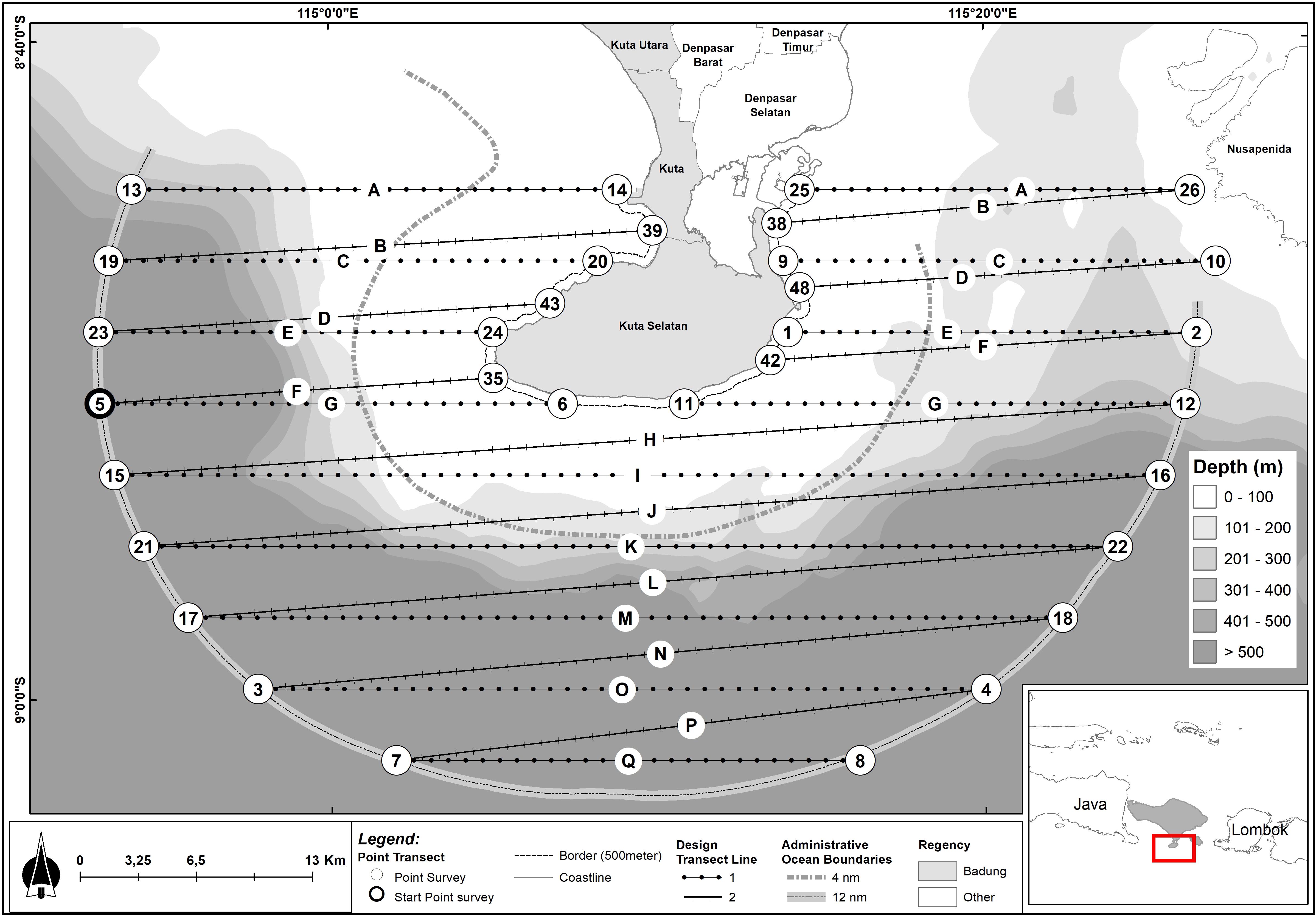
Figure 1. Original design for the line transect survey of Bukit Peninsula, southern Bali.

FIGURE 2

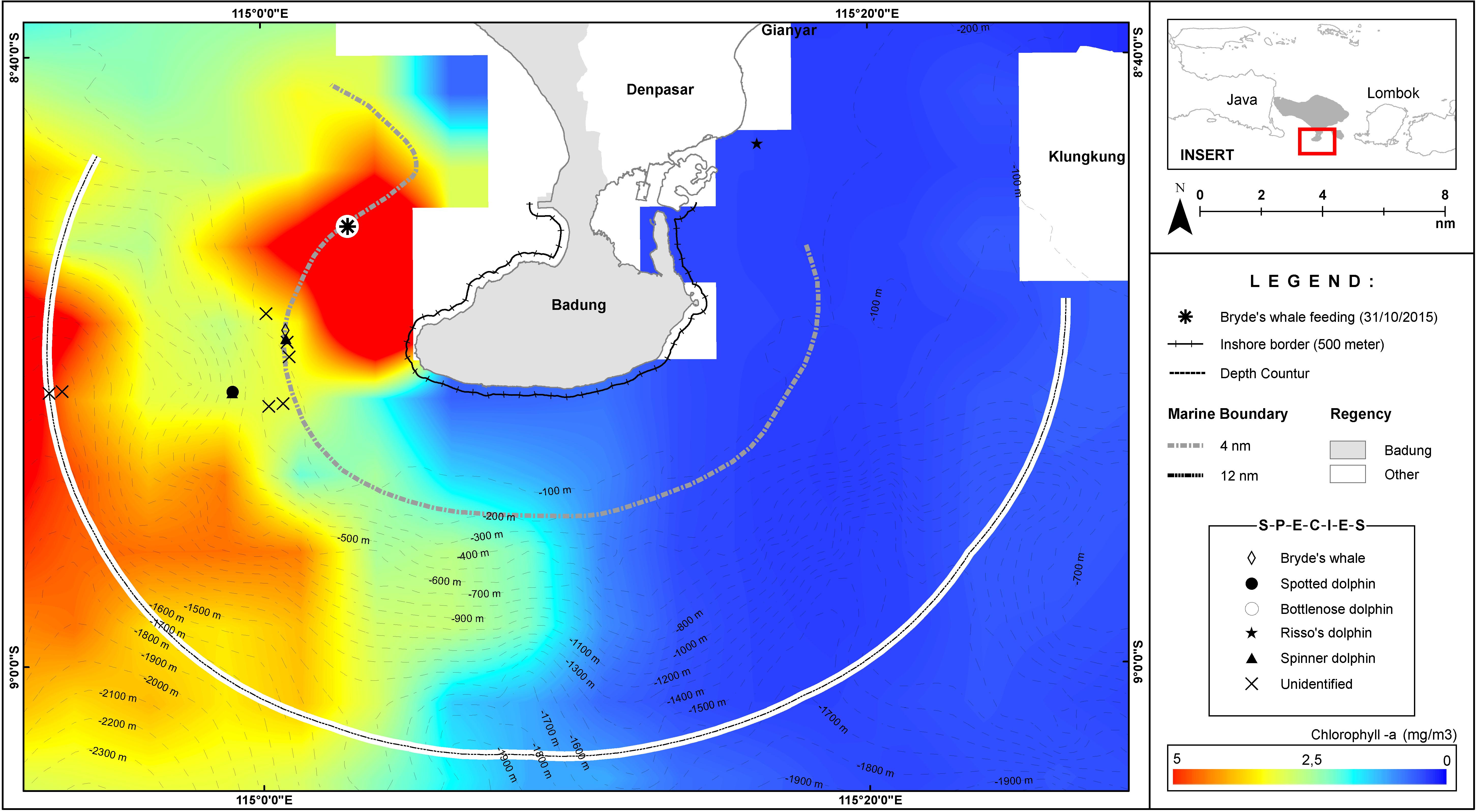
Figure 2. The average chlorophyll-a distribution for October 2015, overlaid with the 31 October 2015 sightings.

FIGURE 3

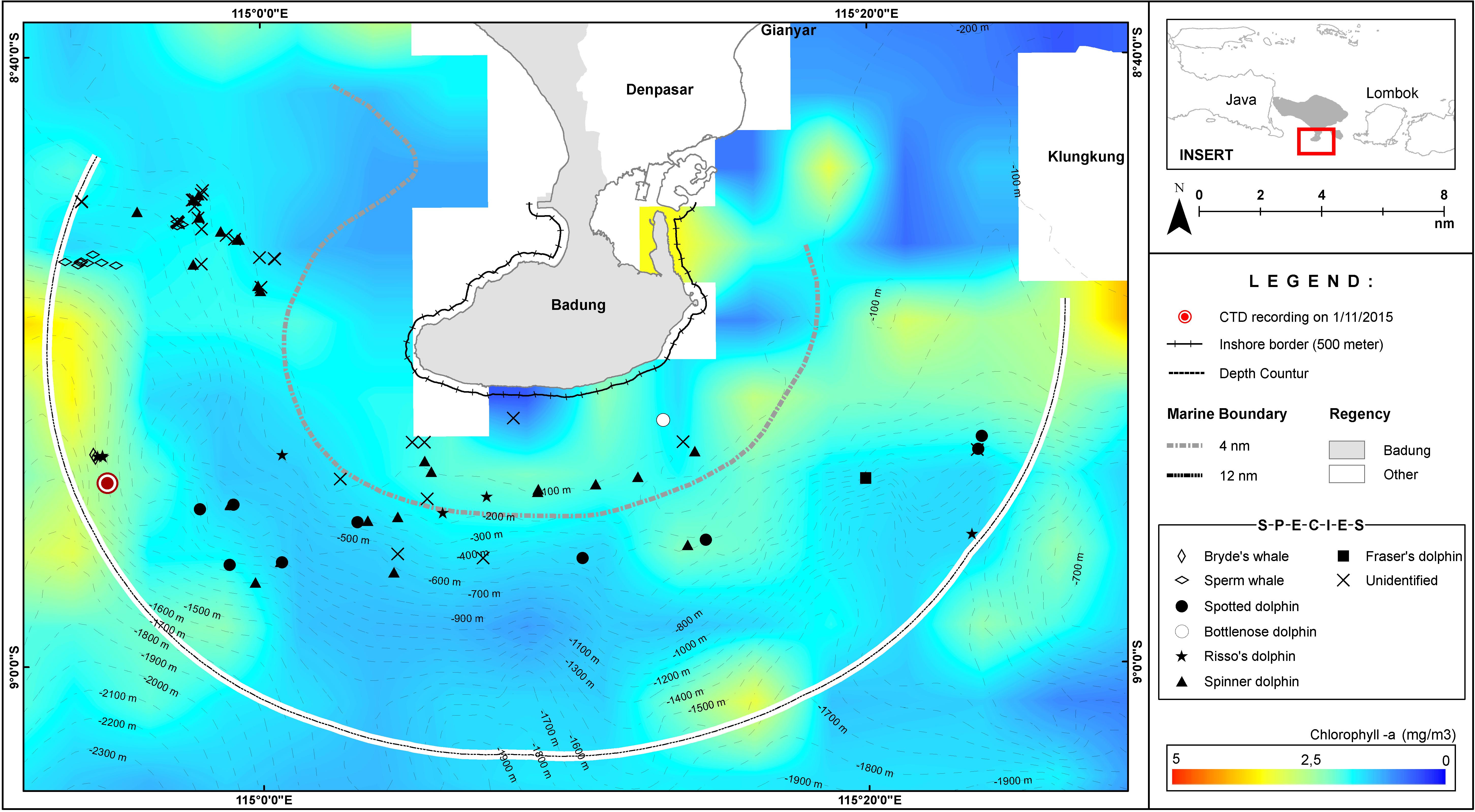
Figure 3. The average chlorophyll-a distribution for November 2015, overlaid with the sightings between 1 and 5 November 2015.

FIGURE 4

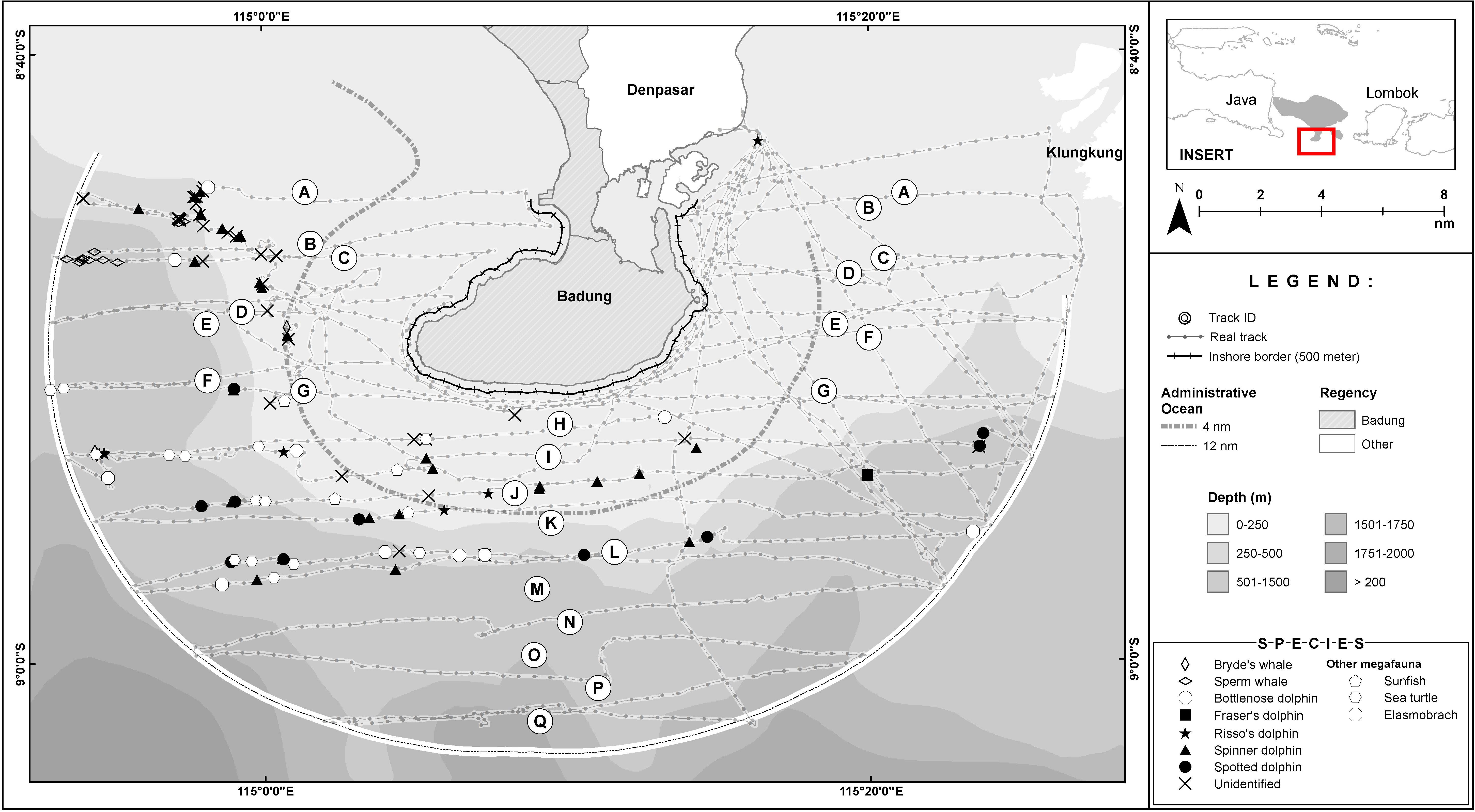
Figure 4. Survey tracks undertaken 30 October to 5 November 2015 during the line transect survey of Bukit Peninsula and dolphins, whales, and other megafauna species recorded within 12 nautical miles (22.2 km) of the Bukit Peninsula. Sightings are plotted over bathymetry data: darker shades indicate increased depth (m). Lines N, O, P, and Q experienced missing data due to a technical issue.

Seasonal upwellings occur in the western and south western parts of the Bali waters. A 2006–2010 dataset indicated sea surface chlorophyll-a concentrations in this region between April to November (Setiawati et al., 2015), while a 2013 dataset indicated Net Primary Productivity for August to October (Rintaka and Priyono, 2020). Conforming to these literatures, Figure 2 captured the average chlorophyll-a productivity in October 2015 while Figure 3 indicates an upwelling on 1 November 2015.

Survey Design and Data Collection

Distance sampling methods estimate the average animal density (number of animals per unit area) in the sampled transects, and use that density estimate to predict the total number of animals in the survey region from which the transects were drawn (Buckland et al., 2001). Assumptions about the “representativeness” of the samples (transects) are met at the design stage (below). Field methods are used to ensure that observers accurately determine animal density along the trackline (below). Typically, 15–20 transects are recommended in order to capture spatial heterogeneity in animal distribution and generate reasonable variance estimates (Buckland et al., 2001).

A small-boat, systematic line transect survey (Williams et al., 2017) was conducted between 30 October and 5 November 2015 over 1,393 sqkm to cover the southern Bukit Peninsula waters. Leaving from the port of Sanur, we designed the line transect survey to use a grid of parallel lines with a random start point, oriented to avoid traveling within the prevailing swell, and joined with a zig-zag to minimize off-effort transit time (Thomas et al., 2007; Figure 1). The survey area covered a range of habitats and prominent environmental gradients, including inshore and offshore waters and shallow and deep waters, in the southern peninsular waters (Figures 1–4). We have also deliberately made the study area boundaries to cover all Bali provincial waters (12 nm, 22 km) for the same reason. Using a 4 km grid spacing and 9–11 kmph boat speed, the final survey design provided even coverage of the survey region using 17 transects (Figure 1). This method follows previous recommendations that even coverage probability can be achieved with an equal-spaced zig zag design of 15–20 samplers and a random start point, while minimizing expensive transit time between tracklines (Strindberg and Buckland, 2004).

Environmental conditions that could influence detection were recorded throughout the survey and as conditions changed (e.g., Beaufort sea state, relative swell height, precipitation, and glare). Some parts of the survey could not be completed due to poor weather (strong winds of Beaufort 5 and above); Figure 4 shows the completed track lines. The Udayana University students carried a Castaway CTD (Conductivity, Temperature and Depth) equipment onboard the research vessel to measure the vertical water temperatures and to detect possible oceanic fronts; with oceanic fronts defined as “an oceanic zone with a strong horizontal gradient in water properties such as temperature, salinity, etc.” (Kida et al., 2016). The CTD was regularly deployed at the starting and ending points of a transect, as well as during sightings. Upon observing the animals, photos were taken to identify their species and behaviors (Objective 1). GPS coordinates were taken to map the distributions of the observed cetacean (Objective 2).

During the survey, an experienced observer (Mustika or Williams) led the data collection each day, and coordinated with the boat driver to survey the track lines as they were planned (Figure 1). When each observer spotted a group of cetaceans, they used an angle board to measure the bearing from the track line to the sighting, and estimated radial distance visually from the track line to the sighting. The experienced observer worked with the observer who made the initial sighting to confirm species identification and estimate group size (best, low, and high). All line transect “effort” (i.e., start and end points of each transect actually surveyed, number of observers, and environmental conditions) and sightings data were collected on a ruggedized Trimble Juno handheld computer running CyberTracker software (Williams et al., 2017). In order to collect data to estimate relative abundance (Objective 3) using distance sampling methods, it was important to collect information on search effort, even when no sightings were made on a given transect. In other words, zeroes are important data points in distance sampling (Buckland et al., 2001).

A joint workshop was held with participants from Udayana University, Conservation International Indonesia, and Oceans Initiative. The workshop introduced 48 faculty members, students, and conservation practitioners to cetacean biology, anthropogenic threats to cetaceans, and provided an overview of the fundamentals of distance sampling. Of these 48 participants, three (one faculty member and two students) rotated through the “training while doing” surveys on the boat (Objective 4).

Data Analysis for the Relative Abundance (Objective 3)

Program Distance (Version 6.2, Release 1; Thomas et al., 2010) was used to analyze detection probability, density, and abundance for all species. In distance sampling, density is the product of the length and width of the surveyed transects. The length of the surveyed area is simply the length of the transect, as measured by GPS. The width is estimated from a family of “detection functions” using the perpendicular distance data from the sightings to each animal. The width of the strip that is effectively searched by the observers can vary according to a number of factors: the size of the animal; the animal’s cryptic or conspicuous behavior; group size; the experience of the observer; the decision to search with binoculars or naked eye, etc. (Buckland et al., 2001). Ideally, one would collect 60–80 sightings of each species, fit separate detection functions for each species, and include factors likely to affect detectability as candidate covariates in a detection function (Buckland et al., 2015). When sample size is inadequate to model detectability as a function of these covariates, one alternative is to rely on a feature of distance sampling of “pooling robustness,” which refers to the fact that distance sampling techniques are robust to the pooling of multiple detection functions into one.

No single species yielded the 60–80 sightings recommended for robust estimation of average detection probability within the effective strip width (Thomas et al., 2010), which is common in pilot studies or surveys of cryptic or rare species (Williams and Thomas, 2009). This small sample size precluded investigation of factors such as environmental conditions that could impact detectability. As a result of small sample size among species, detection functions were fitted to data from three pooled species groups, and then broken down by species assuming equal detectability within the species group. This approach follows previous recommendations for dealing with small sample size or high proportion of sightings that could not be identified to species in the field (e.g., blue and salmon sharks: Williams et al., 2010). The three species groups were as follows: dolphins (bottlenose, Fraser’s, Risso’s, spinner, pantropical spotted, and unknown dolphin); whales (Bryde’s, fin, sperm, and unknown whales); and other large marine megafauna (manta ray, sea snake, shark, turtle, and whale shark).

For each species group, half-normal and hazard rate models were considered. The choice of detection function and truncation distance follows previous recommendations for small boat surveys and rarely seen species (Williams and Thomas, 2007, 2009), but when support for choosing between two models was equivocal (ΔAIC < 2), we averaged on the detection function (Williams and Thomas, 2009). We considered spatial autocorrelation in the density observed among transects in the following way. We used bootstrap methods to estimate variance on the final abundance estimates (“S2 method” in Program Distance; Fewster et al., 2009), because the zig-zag survey design allowed us to treat adjacent pairs of transects as spatially dependent. If the S2 method caused the coefficient of variation to be reduced, we interpreted this as evidence for spatial autocorrelation that we were able to model, and chose the S2 method for estimating variance. If the S2 variance estimator resulted in a higher variance than the analytic variance estimator, then we interpreted this as evidence that there was no clear spatial pattern in density that could be accounted for by treating adjacent pairs of transects as dependent, and therefore used the default (analytic) variance estimator in Distance.

Results

Cetacean Species Diversity and Distribution (Objectives 1 and 2)

During the survey, we observed at least seven species of cetaceans, other marine megafauna and recorded an inventory and sighting location of several avian species. The seven species of cetaceans identified to species by experienced observers were: spinner dolphin (Stenella longirostris), pantropical spotted dolphin (Stenella attenuata), Fraser’s dolphin (Lagenodelphis hosei), Risso’s dolphin (Grampus griseus), bottlenose dolphin (Tursiops sp.), Bryde’s whale (Balaenoptera edeni), and sperm whale (Physeter macrocephalus). All whale sightings occurred off the western side of the Peninsula. Most Bryde’s whale presented in Table 1 were identified from the three ridges on its head (Figure 5A; sensu Shirihai et al., 2006). Eight unidentified whales had the characteristics of the Bryde’s whale (e.g., sickle dorsal fins and sharp deep dive, sensu Shirihai et al., 2006), but since the photographs did not show three ridges due to the whale heads’ positions, we kept these whales “unidentified” (Table 1).

FIGURE 5

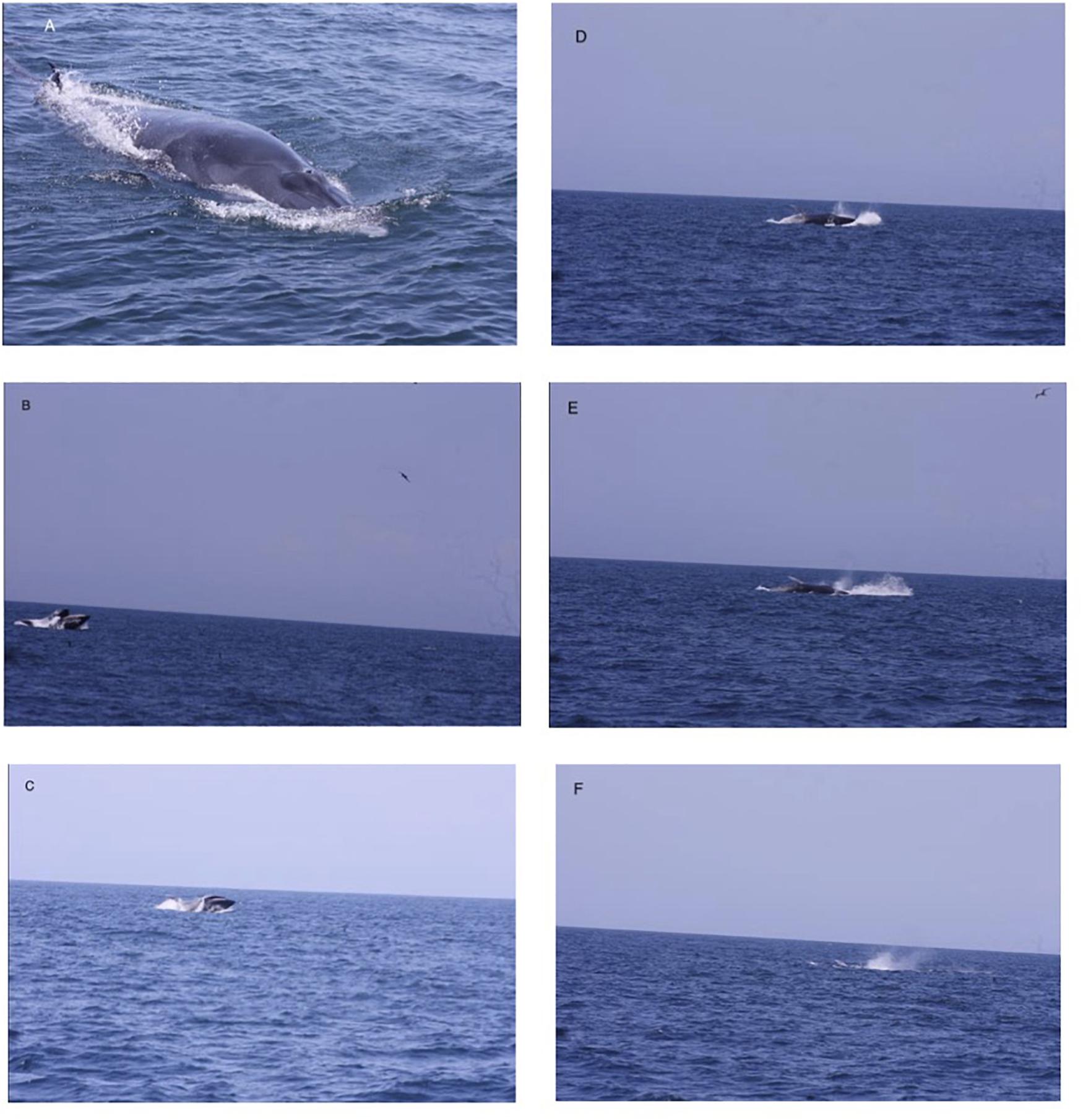
Figure 5. (A) The three ridges on the head of a Bryde’s whale (Balaenoptera edeni). (B) The visible plates of a Bryde’s whale, with a gradation of the lighter white-gray at the front tip and the dark/black plate at the back. (B–F) The lunge feeding sequence of a Bryde’s whale encountered on 31 October 2015 (it did not reorient itself to dive with the dorsal fin exposed per de Mello Neto et al., 2017).

TABLE 1

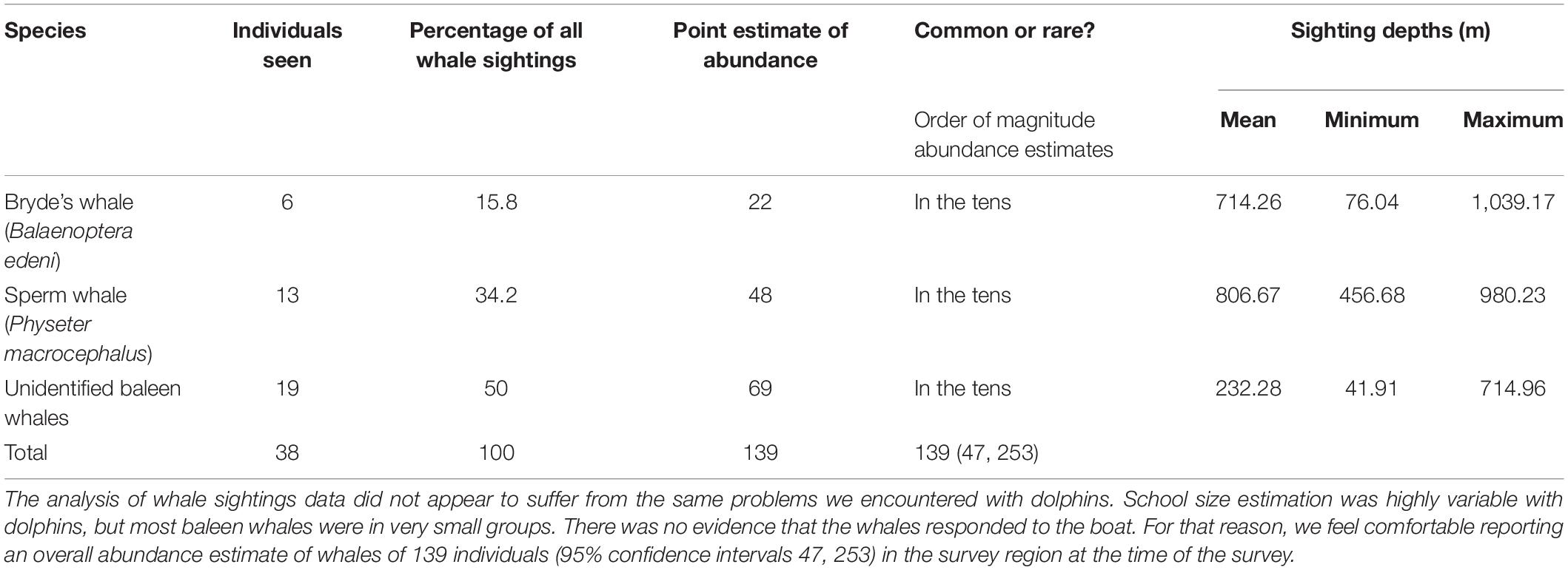
Table 1. Number of sightings used in the detection function analysis for each whale species along with their predicted relative abundance and associated depths in the surveyed region.

The whale and dolphin sightings ranged from shallow water (∼100 m) to deep water (∼ 1,000 m) (Figures 2, 3). The maximum depth of the Fraser’s dolphin sighting was less than 700 m, whereas Risso’s dolphins, spinner dolphins and pantropical spotted dolphins were sighted at the maximum depths of around 1,200 m (Table 2). Both of the maximum depth of the Bryde’s and sperm whales sightings were at around 1,000 m (Table 1). Some dolphins and whales were sighted at 12 nm (22.2 km) from the shoreline. Additional habitat suitability analysis of these sightings will be made in a separate publication.

TABLE 2

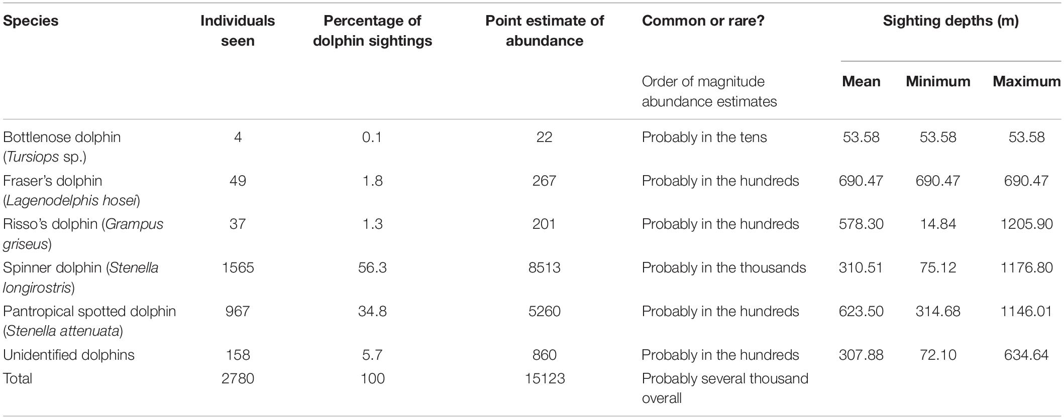
Table 2. Number of sightings used in the detection function analysis for each dolphin species along with their predicted relative abundance and associated depths in the surveyed region.

Feeding behaviors were observed in a Bryde’s whale (see below). On 31 October 2015, one whale was photographed feeding from around 500 m from the survey vessel. This whale was observed feeding, as indicated by its behaviors i.e., lunging while gulping and then twisting (rotating on its lateral axis) before splashing back into the water, but without reorienting dorsal fin position (sensu de Mello Neto et al., 2017; Figures 5B–F). Because the baleen plates of this whale was a gradation of light to dark from the tip of the jaw to the end of the jaw (Figure 5B; sensu Leatherwood et al., 1982), we concluded that it was a Bryde’s whale. Photos of baleen whales were shared with Dr. Gwenith Penry, principal investigator of the Southern African Bryde’s Whale Project, for confirmation.

Many of our sightings happened along marine productivity gradients or oceanic fronts (Figures 3, 4). For instance, the lunge-feeding Bryde’s whale was observed on a productivity gradient on 31 October 2015 (Figure 3). On 1 November 2015 at 11:58 am, our Castaway CTD recorded a sharp thermocline, where the water temperature dropped from 27°C at 0–1 m to 26°C between 1 and 11 m, another drop of 24–26°C between 11 and 12 m and then plunging to 22°C between 12 and 42 m depth (Figure 6). This thermocline indicated upwelling (Ningsih et al., 2013) and thus a relatively rich environment during the time of observation. We observed at least three Bryde’s whales and a manta ray around the time of this sharp thermocline.

FIGURE 6

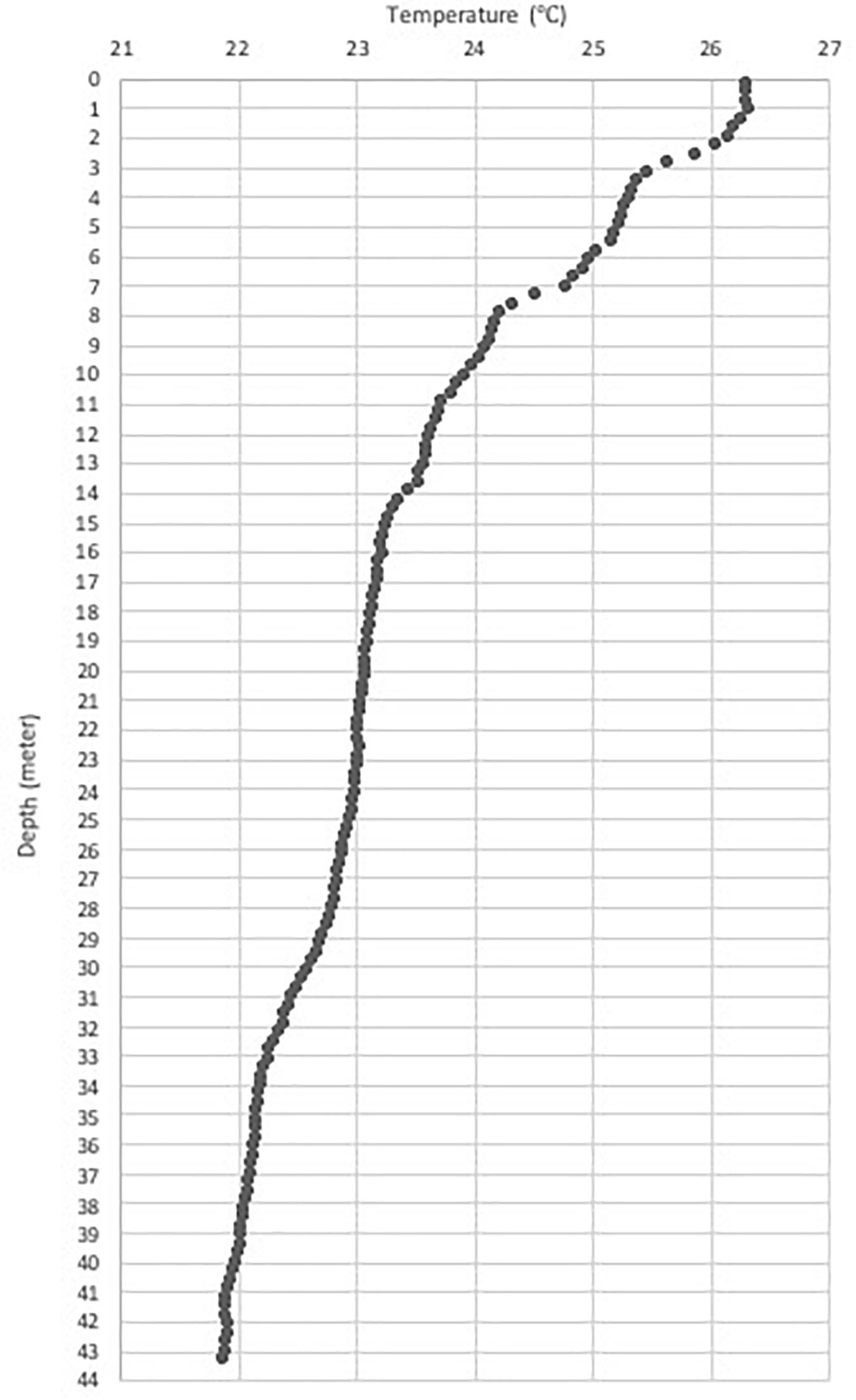
Figure 6. The observed thermocline on 1 November 2015 during sightings of Bryde’s whales and manta rays.

Relative Abundance of the Cetaceans and Presence and Distribution of Other Marine Megafauna (Objective 3)

The survey was completed largely as planned, but a technical problem caused the first day’s worth of data to be lost. This translates to a loss of 4 of the 17 planned transects. The missing data came from the southernmost part of the survey region, so the analyses proceeded as though that portion was not included in the density estimation calculation. The extant data from the 13 covered transects provided reasonable coverage and are thought to be representative of the reduced survey region (Buckland et al., 2001). The area of the reduced survey region, within which abundance was calculated, was 1,393 sq km.

Whales

The hazard rate model failed to converge, so the half-normal model was selected (Figure 7). Truncation of 10% of the largest perpendicular distances was considered, but there was little indication that this improved goodness of fit and would have reduced sample size from 27 to 24 sightings. The decision was made to retain all sightings in the detection function, which had a final average detection probability of 0.40 over an effective strip half-width of 345 m. The chi-square goodness of fit p was 0.539, indicating a good fit to the data. The best estimate of density of all whale species in the region was 0.1 individual per sqkm, which translates to a final estimate of abundance of 139 whales in the survey region. The S2 method yielded higher CVs on density than the analytic variance estimator that treated transects as random samples, so we interpreted this to mean that there was no evidence for spatial dependence in whale density along adjacent transects. The final CV on density (and abundance) was 0.419, which translates into log-normal 95% confidence intervals on abundance of 47–253.

FIGURE 7

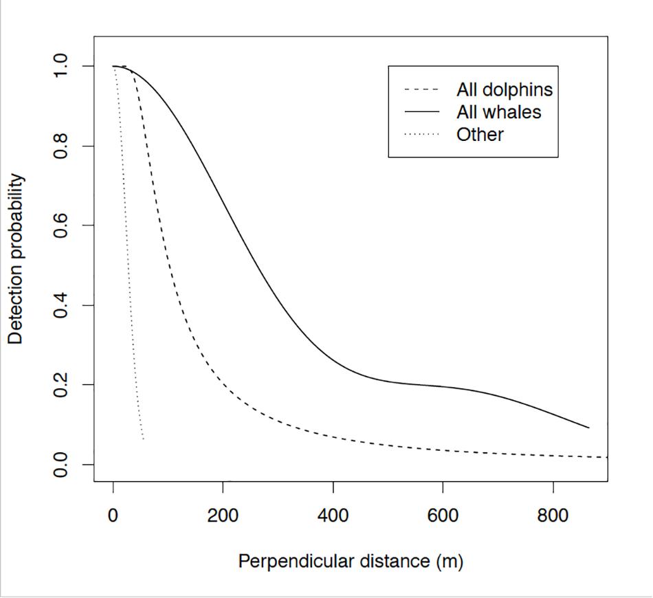
Figure 7. The selected half normal detection function for all surveyed species, pooled as a function of perpendicular distance. Illustrative detection probability of dolphins is represented by a dashed line, whales by a solid line, and of other megafauna by a dotted line. The curves show detection decreasing with increasing perpendicular distance. Detection probability is assumed to be certain [i.e., y (=1)] on the track line [i.e., x (=0)]. Confidence intervals for whales are 47–253.

For illustrative purposes, and assuming equal detectability among whale species, it is possible to use species-specific data on encounter rate to translate the total whale abundance estimate into rough, tentative estimates of abundance of that species in the survey region. Using the best estimate of group size for each sighting, the observers recorded on-effort sightings of 38 individual whales in 30 sightings. Table 1 shows how these sightings were broken down by species, and how those percentages translate into rough predictions of abundance.

Dolphins

There was strong support from the data for choosing the hazard rate model over the half-normal model (ΔAIC = 2.08; Figure 7), but behavioural observations in the field suggested that dolphins responded to the presence of the boat to ride the boat’s bow waves. Consequently, the spike near zero perpendicular distance was interpreted as evidence of responsive movement, rather than evidence that observers were covering a very narrow strip width. Following previous recommendations for bow-riding Pacific white-sided dolphins (Williams and Thomas, 2007), a half-normal detection function was used to avoid overfitting the spike. Truncating 10% of sightings with the largest perpendicular distances was considered, but there was little indication that this improved goodness of fit, reduced the sample size from 64 to 58 sightings, and caused a substantial (0.1) increase in CV. The decision was made to retain all sightings in the detection function, resulting in a final average detection probability of 0.26 over an effective strip half-width of 237 m. The best estimate of density of all dolphin species in the region was 11 individuals per sqkm, which translates to a final abundance estimate of 15,323 dolphins in the survey region. The S2 variance method suggested spatial dependence of density in pairs of zig-zag samplers. The final CV on density (and abundance) was 0.39, which translates into log-normal 95% confidence intervals on abundance of 7,138–32,040.

For illustrative purposes, and assuming equal detectability among species, it is possible to use the species-specific encounter rate to translate the total number of dolphins in the region into rough, tentative estimates of abundance of that species. Using the best estimate of group size for each sighting, the observers recorded on-effort sightings of 2,780 individual dolphins in 64 schools. Table 2 shows how these sightings were broken down by species, and how those percentages translate into rough predictions of abundance.

Other Marine Megafauna

Other marine megafauna observed include sea turtles (green turtles/Chelonia mydas and possibly Olive Ridley turtles/Lepidochelys olivacea), sunfish (Mola sp.), manta rays (Mobula birostris), a whale shark (Rhincodon typus), an unidentified reef shark and an unidentified sea snake (Table 3). Avian species encountered were Christmas frigatebird (Fregata andrewsi), lesser frigatebird (Fregata ariel), Great crested tern (Sterna bergii), little tern (Sterna albifrons), little pied cormorant (Phalacrocorax melanoleucos), red-necked phalarope (Phalaropus lobatus), Wilson’s storm petrel (Oceanites oceanicus), but no attempt was made to record perpendicular distances or fit a detection function for birds. The hazard rate model failed to converge, so the half-normal model was selected to estimate the effective strip width for “other marine megafauna” (Figure 7). A truncation of 10% of the largest perpendicular distances improved goodness of fit (from p = 0.000 for the untruncated data to p = 0.223 for the truncated data). Although truncation of 10% of sightings reduced sample size from 32 to 29 sightings, goodness of fit statistics guided the final decision to truncate sightings. The selected detection function had an average detection probability of 0.51 over an effective strip half-width of 29 m. The chi-square goodness of fit p was 0.223, indicating a good fit to the data. The best estimate of density of other marine megafauna in the region was 0.9 individuals per sqkm, which translates to a final estimate of abundance of 1,253 animals in the survey region. The S2 method revealed no evidence for spatial dependence in other marine megafauna density along pairs of adjacent transects. The final CV on density (and abundance) was 0.326, which translates into log-normal 95% confidence intervals on abundance of 614–2,346.

TABLE 3

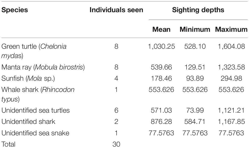
Table 3. Number of sightings for each additional megafauna species in the surveyed region.

Discussion

Cetacean Species Diversity (Objective 1)

The survey achieved its primary objectives of collecting valuable effort and cetacean sightings data, while strengthening local capacity for marine biodiversity monitoring. The survey resulted in a documented inventory of cetacean species in the region during the wet season, but we recognize that the survey may need to be repeated several times, including in the dry season, to detect rare species (Kaschner et al., 2012). From the perspective of biodiversity, the survey adds Fraser’s dolphin to the list of cetaceans observed around the Bukit Peninsula waters, thus Bali now has nine cetacean species in the southern Peninsular waters. Seven of the Peninsular species were observed during the survey (Tables 1, 2) while two of them (the killer whale Orcinus orca and the false killer whale Pseudorca crassidens) were not observed during the survey.

From the viewpoint of large whale conservation, this survey proves the importance of the study area as the habitats of sperm whales and Bryde’s whales. Sperm whales are one of the most often stranded marine mammals in Indonesia with 64 recorded events from 1997 to 2021; nine of them happened in Balinese waters (see text footnote 1). Our survey further confirms the importance of southern Bali waters as a habitat of sperm whales.

Cetacean Species Distribution (Objective 2)

The spatial information is of great value to local conservation practitioners engaged in place-based marine spatial planning and conservation efforts. The survey generated rich data for the design of the Badung Marine Protected Area and, more broadly, for coastal zone management in the region. We observed a Bryde’s whale feeding at an ocean front on 31 October 2015 (Figure 2) and a thermocline-induced upwelling on 1 November 2015 (Figure 6), thus corroborating the knowledge that the southern waters of Bali are still productive in October and early November (Ningsih et al., 2013; Setiawati et al., 2015; Rintaka and Priyono, 2020). Some dolphins and whales were observed quite far from the shoreline (12 nm or 22.2 km, Figures 2–4), indicating that the Badung MPA outer boundary needs to be designed to cover these limits. Due to the likely importance of the Bukit Peninsula as a cetacean habitat, the data from this survey has now been accommodated into the draft marine spatial plan of the Bali Province, proposing that the waters of the Bukit Peninsula be assigned as a conservation area. The draft marine spatial plan for Bali is expected to be completed by the end of 2021.

The southern waters of Bali could be an important habitat for the Bryde’s whale. Four Bryde’s whales stranding events have been recorded in south Bali in August 2010, February 2016, May 2016 and January 2021. The 2 February 2016 stranding involved a live 3.28 m female Bryde’s whale calf at Batubolong, Canggu, ∼30 km north of the Bryde’s whale sighting site in November 2015 (ID 261 of www.whalestrandingindonesia.com; Whale Stranding Indonesia, 2013). The emaciated Bryde’s whale calf died during rescue and was immediately necropsied by a team led by the Udayana University in Denpasar. No milk was found in the gastro-intestinal tract of the whale, suggesting that she had not suckled her mother, or was just recently suckling the mother when they were separated for unknown reasons. Given the uncertainty in migratory patterns of Bryde’s whale in tropical waters and recognizing that some populations may not migrate between breeding and feeding grounds (Clapham et al., 1999; Thomas et al., 2016), the observation of a Bryde’s whale feeding at an ocean front in the study area is important. This observation can strengthen local citizen science efforts to improve our understanding of the way that Bryde’s whales use their habitat around the Peninsula (i.e., for feeding, breeding, or both).

The Relative Abundance of Cetaceans and Presence of Other Marine Megafauna (Objective 3)

The relative abundance analysis of dolphins as a whole yields a very large estimate of abundance that strikes us as implausibly high. We can interpret the extremely high number of dolphins in a number of ways, not mutually exclusive.

The first interpretation is that perhaps the dolphin density truly is high in the region. In one of the largest cetacean surveys anywhere, long-term monitoring of dolphin populations in the eastern tropical Pacific resulted in a total of 9.6 million delphinids in a 19 million sqkm study area (0.50 dolphins per sqkm; Wade and Gerrodette, 1993). The dolphin density we report (11 dolphins per sqkm) is much higher than the mean density (0.50 dolphins per sqkm) reported from the ETP (Wade and Gerrodette, 1993). Best et al. (2015) fitted spatially explicit density surface models to line transect effort and marine mammal sightings data, and found that the highest-density sites in British Columbia, Canada did contain ∼10 Pacific white-sided dolphins per sqkm. Surveys for two species of freshwater dolphins in the Amazon found that preferred habitats had dolphin densities of 2–5 dolphins per sq km (Williams et al., 2016b). Taken as a whole, it seems implausible that the dolphin density we report is real, but it is not impossible.

The second interpretation is that our estimate of dolphin density in the sampled transects is biased high. Several factors indicate that the density estimate produced an overestimate of dolphin density along the track-line. This low-cost, small-boat survey led us to violate some key assumptions of conventional distance sampling (Buckland et al., 2015).

The first assumption of the second interpretation is that the perpendicular distances (or radial distances and angles) to sightings are measured without error. The budget allowed for only a few days’ of boat time, so protocols relied on training observers to judge distance. Future iterations of this survey could allocate a few days in the field to conduct distance estimation experiments to account for inter-observer differences in visual estimation to remove bias, or, if a higher survey platform were available, reticles or photogrammetry methods could be used to measure distance to cetaceans (Williams et al., 2007; Dawson et al., 2008).

The second assumption of the second interpretation is that the observers recorded the distance and angle to each sighting before the animals have responded to the boat (i.e., either avoidance, which would bias density estimates low, or attraction, which would bias density estimates high; Buckland et al., 2015). The spike in the dolphin detection function near zero convinces us that, at a minimum, dolphins approaching the vessel resulted in some unknown degree of overestimation of dolphin abundance. Statistical methods are available to account for responsive movement (Palka and Hammond, 2001), but we were unable to collect suitable data. Future surveys would benefit from a higher survey platform to allow observers to search well ahead of the vessel, especially given the swell.

The third assumption of the second interpretation is that group sizes are correctly estimated. Overestimation of group sizes will result in overestimation of overall abundance. We have no way of testing this from our data, but it does seem plausible. Some observers had never seen dolphins before, and could easily have overestimated the group size of highly social dolphins (i.e., in contrast to the baleen whales, which were usually solitary). In any “training while doing” survey, there will be a tradeoff between training new observers and collecting reliable data. The balance we struck in this survey was acceptable to end-users of the science for the purposes of co-generating knowledge for our application, because the questions we were asking relied primarily on spatial data to inform an MPA design. A different balance would be needed if management decisions rely on estimates of absolute abundance. Future surveys could use a drone to collect aerial photographs of schools to improve estimates of school size, or generate a correction factor for each observer to quantify the degree to which some observers over- or under-estimated group size, on average.

The absence of cetacean sightings between Benoa and the Nusa Penida Islands was surprising. The marine traffic intensity between Benoa and Nusa Penida and the number of vessels coming into and out of Benoa Harbour to other parts of Indonesia may play a role in the absence of cetacean sightings during this survey. Qualitative interviews with vessel operators and fishers on cetacean sightings between Benoa Harbour and Nusa Penida might be worthwhile to obtain the historical perspectives of cetacean abundance in this region. In addition, analyses of the average chlorophyll-a distribution during October and November 2015 (Figures 2, 3, respectively) show a higher productivity on the western side of the Peninsula, although it was mainly in the month of October. On the other hand, in both months, the waters between Benoa and Nusa Penida were much less productive than the western side of the Peninsula. The combination of productivity and marine traffic intensity may have contributed to the absence of observed cetaceans in the eastern part of the study area.

The survey resulted in new and unexpected co-generated knowledge on other marine megafauna. We do not feel comfortable reporting estimates of density or abundance, because these taxa (i.e., sharks, mantas, turtles, and sea snakes) all violated the assumption that all animals are visible at the surface and available for detection [i.e., the so-called “g(0) = 1” assumption; Buckland et al., 2015]. However, we do see value in pointing out the frequency of sightings of some of these animals, which are particularly noteworthy in light of the very narrow effective strip width observers covered for that taxonomic group (Figure 7). The absolute number of sightings of whales, dolphins, and other marine megafauna give one kind of information on commonness and rarity, but these must be interpreted in light of the large differences in detectability among taxa (Figure 7). As expected from body size, we covered the widest effective strip width for whales, then dolphins, then other marine megafauna (Figure 7).

Although the survey did not generate abundance estimates for all taxa, they provide information that can be helpful in designing future surveys to make them more statistically powerful and cost effective. It is common in surveys of cryptic or rare species, by teams working with little funding for ship time, that abundance estimates may emerge over time as survey design improves, observers gain access to additional training, and sample sizes increase to allow more sophisticated analyses (Williams et al., 2016b). By taking the region from “no data” to “some data,” the survey has made a valuable contribution to long-term conservation and management plans.

The Indonesia Through Flow and the seasonal upwelling (June–October) in southern Bali (Ningsih et al., 2013) might have contributed to the very high number of marine megafauna in the region. It is possible that the cetaceans were sighted when the Peninsular water was in high productivity, as indicated by Bryde’s whale and spinner dolphin feeding behaviors. The examination of the abundance of the cetaceans and other marine megafauna during much lower productivity months (e.g., around March or April) is thus recommended.

Lessons Learned From the Training (Objective 4) and Future Research and Actions

From our perspective, the most valuable feature of the study is that the knowledge was “co-generated” (Norström et al., 2020) by a diverse group of scientists and observers in a “training while doing” framework, which allowed us to collect a systematic snapshot of local marine biodiversity while building capacity to do marine biodiversity monitoring in future (Williams et al., 2017). The two student participants were able to use the data in their undergraduate research, and overall, the project offered a legacy of increased local capacity to record marine mammal observations for research or industry applications. The collaboration with the Udayana University has proven useful because it provided the team with knowledge and expertise from both the Marine Sciences and Veterinary faculties of the university. The two students have since then finished their undergraduate degree. Purba observed the dolphins in Tejakula, an emerging dolphin watching site in east Bali, for his undergraduate thesis project and he is currently finishing his masters degree on Indonesian maritime security. Maharta modeled the rates and distributions of sedimentation in the Benoa Bay for his undergraduate project and has also finished his masters degree on the oceanographic modeling of plastic waste at sea. Both former students agree that their participation in this study has helped widening their horizon on their career options, as well as what marine science can do to improve Indonesia’s environmental conservation.

One of the best outcomes of our survey was the knowledge sharing between Western researchers and local experts (Norström et al., 2020). The survey began with a prayer and offering at the Balinese Hindu sea temple, Uluwatu. This ritual led to several discussions of the need to improve our understanding of the level and impacts of ocean noise in the region, with a recognition that doing so could improve the selection, design, and management of Badung Marine Protected Area as a “Quiet(er) MPA” (Williams et al., 2015). These discussions inspired us to return to the area with calibrated, autonomous hydrophones to measure ocean noise levels throughout the region, leading to the surprising discovery that airplane noise was a significant contributor to underwater noise levels in western Peninsular waters (Erbe et al., 2018). These discussions also identified Nyepi (Day of Silence), the Balinese Hindu New Year, as a potential opportunity for a natural experiment to measure changes in ocean noise when ports, the airport, and stores are closed for one day. When we returned to measure ocean noise levels before, during, and after Nyepi, we found that levels dropped substantially on the day when communities along the Bukit Peninsula Honoured Nyepi (Williams et al., 2018). This local knowledge was invaluable to quantifying an important anthropogenic threat to cetaceans, namely ocean noise, but the knowledge would not have been incorporated into our science without a knowledge co-production framework (Lam et al., 2020). As communities develop management plans for the Badung MPA, there is strong interest in including spatial and temporal aspects of chronic ocean noise into the management plan. Formalizing a Nyepi no-trespass policy in provincial waters would provide a quieter zone for cetaceans in Bali and raise awareness on ocean noise.

Evidence of bycatch has also been recorded during our study. During transect surveys carried out in November 2015, a spinner dolphin calf was found with an amputated fluke. Bycatch is not quantified in the region (but see Anderson et al., 2020), and should be further investigated in the future.

As we continue this work, there will be a need to strengthen our ability to estimate abundance, or at least minimum abundance, and bycatch mortality rates of small cetaceans to assess sustainability of fisheries bycatch (Read et al., 2006; Reeves et al., 2013). Due to the unknown odds of detecting a bycatch event during a line transect survey in a poor-bycatch data region, a concerted effort is needed to place observers on fishing boats to generate robust estimates of bycatch mortality rates, and to build capacity among local fishers to mitigate bycatch. Local capacity to conduct surveys to estimate cetacean abundance and bycatch mortality rate is needed urgently, in order to allow Indonesian seafood exports continued access to United States seafood markets. A new United States seafood import rule will require exporting nations to ensure that their fisheries management is comparable in effectiveness to the United States Marine Mammal Protection Act with respect to assessing and mitigating marine mammal bycatch (Williams et al., 2016a). The design and training in this line transect survey is a good starting point to build a better scientific capability to estimate abundance and distribution of cetaceans in a productive, but understudied region. Our future work will require rapid assessment of bycatch rates, in order to help Indonesia build the evidence for the sustainability of bycatch in their export fisheries before the rule comes into effect on January 1, 2022 (Punt et al., 2021). Although the import rule does not apply to domestic, artisanal, or subsistence fisheries, commercial seafood exports to United States exceeded USD$1 billion in 2015 (Williams et al., 2016a), so there is a strong incentive to build scientific capacity in the country to assess the size of marine mammal populations in Indonesian waters to assess whether bycatch is sustainable.

We compare the presence of Bryde’s whale in our study area with several Important Marine Mammal Areas (IMMAs) which have been delineated in consultation with Indonesian experts. IMMAs are “areas identified as important for a marine mammal population” with the purpose of ensuring favorable conservation status of marine mammals within those IMMAs (Marine Mammal Protected Areas Task Force, 2021a). The southern Peninsular waters of Bali is part of the “Southern Bali Peninsula and Adjacent Slope” IMMA (Marine Mammal Protected Areas Task Force, 2021b), where Bryde’s whales have been listed as a focal species to conserve. Bryde’s whales have also been observed west of Lovina in the Buleleng waters of north Bali (Mustika, personal observation, currently listed as the Buleleng IMMA), indicating that the island Province of Bali may play an important role in the conservation of this species. Bryde’s whales have also been observed in the Wakatobi National Park (Sahri et al., 2020; the Wakatobi IMMA), Raja Ampat in West Papua (Ender et al., 2014; candidate IMMA) and Savu Sea and Surrounding Areas IMMA (Marine Mammal Protected Areas Task Force, 2021c). The confirmed sightings of Bryde’s whales in this study, and the likelihood that eight out of 19 unidentified baleen whales (Table 1) were also Bryde’s whales, add to the postulation that the study area is an important feeding habitat and a possible breeding or nursing ground for this species. We intend to add a photo-identification and genetic component to future research, in order to investigate site-fidelity, residence times, and stock definition of this poorly studied species.

Future surveys should also focus on addressing limitations so that reliable abundance estimates can be produced, and continued monitoring over longer time scales would allow for more complex analyses, such as density surface models (Thomas et al., 2010; Buckland et al., 2015). Doing so will allow us to consider spatial and temporal trends in marine biodiversity, and help us understand whether management actions, including designation of an MPA, are achieving the desired conservation effects.

Data Availability Statement

The datasets presented in this article are not readily available because the dataset belongs to Conservation International Indonesia which prohibits the authors from releasing the data. Any parties in need of the data should contact Conservation International Indonesia. Requests to access the datasets should be directed to ID.

Ethics Statement

Ethical review and approval was not required for the animal study because when the research was conducted, ecological research in Indonesia did not require any research permits.

Author Contributions

PM andRWconceived of the study and prepared the manuscript. PM, RW, HK, AP, IM, and EF collected the data. RW analyzed the data. DR analyzed the bycatch necropsy. ID supervised the project and aligned the project with the greater umbrella of the Bali MPA Network.

Funding

Research funding was provided by an anonymous donor via Conservation International Indonesia. The development of Oceans Initiative’s Animal Counting Toolkit program was supported with grants over several years from Synchronicity Earth, Marisla Foundation, and the US Marine Mammal Commission. Oceans Initiative provided the funding for the publication of this paper.

Conflict of Interest

The authors declare that the research was conducted in the absence of any commercial or financial relationships that could be construed as a potential conflict of interest.

Acknowledgments

We would like to acknowledge donor to Conservation International Indonesia, whose support was essential to completing this research. RW thanks Synchronicity Earth, Marisla Foundation, and the US Marine Mammal Commission for supporting the development of the Animal Counting Toolkit program of Oceans Initiative. We thank Kimberly Nielsen, Andrea Mendez-Bye, Stephanie Reiss, and Catherine Lo for editorial assistance. We thank two reviewers and editor JK for the very helpful feedback on the manuscript. We also thank Dr. Asha de Vos for the fruitful discussions on avoiding parachute science in international collaborations.

Footnotes

1. ^ www.whalestrandingindonesia.com

References

Anderson, R. C., Herrera, M., Ilangakoon, A. D., Koya, K. M., Moazzam, M., Mustika, P. L., et al. (2020). Cetacean bycatch in Indian Ocean tuna gillnet fisheries. Endanger. Species Res. 41, 39–53. doi: 10.3354/esr01008

CrossRef Full Text | Google Scholar

Beasley, I., Jedensjö, M., Wijaya, G. M., Anamiato, J., Kahn, B., and Kreb, D. (2016). Observations on Australian humpback dolphins (Sousa sahulensis) in waters of the Pacific Islands and New Guinea. Adv. Mar. Biol. 73, 219–271. doi: 10.1016/bs.amb.2015.08.003

PubMed Abstract | CrossRef Full Text | Google Scholar

Best, B. D., Fox, C. H., Williams, R., Halpin, P. N., and Paquet, P. C. (2015). Updated marine mammal distribution and abundance estimates in British Columbia. J. Cetacean Res. Manage. 15, 9–26.

Google Scholar

Bowen, W. D. (1997). Role of marine mammals in aquatic ecosystems. Mar. Ecol. Prog. Ser. 158, 267–274. doi: 10.3354/meps158267

CrossRef Full Text | Google Scholar

Buckland, S. T., Anderson, D. R., Burnham, K. P., Laake, J. L., Borchers, D. L., and Thomas, L. (2001). Introduction to Distance Sampling: Estimating Abundance of Biological Populations. Oxford: Oxford University Press.

Google Scholar

Buckland, S. T., Rexstad, E. A., Marques, T. A., and Oedekoven, C. S. (2015). Distance Sampling: Methods and Applications. Cham: Springer International Publishing.

Google Scholar

Chami, R., Cosimano, T., Fullenkamp, C., and Oztosun, S. (2019). Nature’s solution to climate change. Finance Dev. 56, 34–38.

Google Scholar

Clapham, P. J., Young Sharon, B., and Brownell, R. L.Jr. (1999). Baleen whales: conservation issues and the status of the most endangered populations. Mamm. Rev. 29, 37–62. doi: 10.1046/j.1365-2907.1999.00035.x

CrossRef Full Text | Google Scholar

Dawson, S., Wade, P., Slooten, E., and Barlow, J. (2008). Design and field methods for sighting surveys of cetaceans in coastal and riverine habitats. Mamm. Rev. 38, 19–49. doi: 10.1111/j.1365-2907.2008.00119.x

CrossRef Full Text | Google Scholar

de Mello Neto, T., de Sá Maciel, I., Tardin, R. H., and Simão, S. M. (2017). Twisting Movements During Feeding Behavior by a Bryde’s Whale (Balaenoptera edeni) Off the Coast of Southeastern Brazil. Aquat. Mamm. 43, 501–506. doi: 10.1578/am.43.5.2017.501

CrossRef Full Text | Google Scholar

Ender, A. I., Mangubhai, S., Wilson, J. R., and Muljadi, A. (2014). Cetaceans in the global centre of marine biodiversity. Mar. Biodivers. Rec. 7:E18.

Google Scholar

Erbe, C., Williams, R., Parsons, M., Parsons, S. K., Hendrawan, I. G., and Dewantama, I. M. I. (2018). Underwater noise from airplanes: an overlooked source of ocean noise. Mar. Pollut. Bull. 137, 656–661. doi: 10.1016/j.marpolbul.2018.10.064

PubMed Abstract | CrossRef Full Text | Google Scholar

Fewster, R. M., Buckland, S. T., Burnham, K. P., Borchers, D. L., Jupp, P. E., Laake, J. L., et al. (2009). Estimating the encounter rate variance in distance sampling. Biometrics 65, 225–236. doi: 10.1111/j.1541-0420.2008.01018.x

PubMed Abstract | CrossRef Full Text | Google Scholar

Kabar24 (2014). Benoa Targetkan 62 Kapal Pesiar Mulai 2015. Available online at: https://kabar24.bisnis.com/read/20141001/78/261626/benoa-targetkan-62-kapal-pesiar-mulai-2015 (accessed February 19, 2021).

Google Scholar

Kaschner, K., Quick, N. J., Jewell, R., Williams, R., and Harris, C. M. (2012). Global coverage of cetacean line-transect surveys: status quo, data gaps and future challenges. PLoS One 7:e44075. doi: 10.1371/journal.pone.0044075

PubMed Abstract | CrossRef Full Text | Google Scholar

Katona, S., and Whitehead, H. (1988). Are cetacea ecologically important. Oceanogr. Mar. Biol. 26, 553–568.

Google Scholar

Kida, S., Mitsudera, H., Aoki, S., Guo, X., Ito, S. I., Kobashi, F., et al. (2016). “Oceanic fronts and jets around Japan: a review,” in Hot Spots in the Climate System: New Developments in the Extratropical Ocean-Atmosphere Interaction Research, eds H. Nakamura, A. Isobe, S. Minobe, H. Mitsudera, M. Nonaka, and T. Suga (Tokyo: Springer), 1–30. doi: 10.1007/978-4-431-56053-1_1

CrossRef Full Text | Google Scholar

Lam, D. P. M., Hinz, E., Lang, D. J., Tengö, M., von Wehrden, H., and Martín-López, B. (2020). Indigenous and local knowledge in sustainability transformations research: a literature review. Ecol. Soc. 25:3. doi: 10.5751/ES-11305-250103

PubMed Abstract | CrossRef Full Text | Google Scholar

Lavery, T. J., Roudnew, B., Gill, P., Seymour, J., Seuront, L., Johnson, G., et al. (2010). Iron defecation by sperm whales stimulates carbon export in the Southern Ocean. Proc. Biol. Sci. 277, 3527–3531. doi: 10.1098/rspb.2010.0863

PubMed Abstract | CrossRef Full Text | Google Scholar

Leatherwood, S., Reeves, R. R., Perrin, W. F., and Evans, W. E. (1982). Whales, Dolphins, and Porpoises of the Eastern North Pacific and Adjacent Waters. NOAA Technical Report NMFS Circular. (Rockville, MD: Dover Publications), 1–245.

Google Scholar

Margules, T. (2011). Understanding and Valuing the Role of Ecosystem Services in the Economy of Uluwatu, Bali, Indonesia. Honours thesis. Lismore: Southern Cross University.

Google Scholar

Marine Mammal Protected Areas Task Force (2021a). Basics on IMMAs. Available online at: https://www.marinemammalhabitat.org/immas/faq-on-immas/ (accessed February 25, 2021).

Google Scholar

Marine Mammal Protected Areas Task Force (2021b). Savu Sea and Surrounding Areas IMMA. Available online at: https://www.marinemammalhabitat.org/immas/faq-on-immas/ (accessed February 25, 2021).

Google Scholar

Marine Mammal Protected Areas Task Force (2021c). Southern Bali Peninsula and Adjacent Slope IMMA. Available online at: https://www.marinemammalhabitat.org/portfolio-item/southern-bali-peninsula-slope/ (accessed February 25, 2021).

Google Scholar

Morissette, L., Hammill, M. O., and Savenkoff, C. (2006). The trophic role of marine mammals in the northern Gulf of St. Lawrence. Mar. Mamm. Sci. 22, 74–103.

Google Scholar

Mustika, P. L., Ratha, I. M. J., and Purwanto, S. (eds) (2011). The 2011 Bali Marine Rapid Assessment (Kajian Cepat Kondisi Kelautan Propinsi Bali 2011). Denpasar: Universitas Warmadewa.

Google Scholar

Mustika, P. L. K. (2011). Towards Sustainable Dolphin Watching Tourism in Lovina, Bali, Indonesia. Ph.D. thesis. Townsville: James Cook University.

Google Scholar

Mustika, P. L. K., Birtles, A., Everingham, Y., and Marsh, H. (2013). The human dimensions of wildlife tourism in a developing country: watching spinner dolphins at Lovina, Bali, Indonesia. J. Sustain. Tour. 21, 229–251. doi: 10.1080/09669582.2012.692881

CrossRef Full Text | Google Scholar

Mustika, P. L. K., and Ratha, I. M. J. (2013). Towards a Bali MPA. Bali Marine Rapid Assessment Program 2011. Available online at: https://bioone.org/ebooks/RAP-Bulletin-of-Biological-Assessment/Bali-Marine-Rapid-Assessment-Program-2011/eISBN-/10.1896/978-1-934151-51-8 (access September 10, 2021).

Google Scholar

Mustika, P. L. K., Sadili, D., Sunuddin, A., Kreb, D., Hadi, S., Ramli, I., et al. (2016). Rencana Aksi Nasional (RAN) Konservasi Cetacea Indonesia 2016-2020 (the Cetacean National Plan of Action (NPOA) for Indonesia 2016-2020). Jakarta: Ministry of Marine Affairs and Fisheries.

Google Scholar

Ningsih, N. S., Rakhmaputeri, N., and Harto, A. B. (2013). Upwelling variability along the southern coast of Bali and in Nusa Tenggara waters. Ocean Sci. J. 48, 49–57. doi: 10.1007/s12601-013-0004-3

CrossRef Full Text | Google Scholar

Norström, A. V., Cvitanovic, C., Löf, M. F., West, S., Wyborn, C., Balvanera, P., et al. (2020). Principles for knowledge co-production in sustainability research. Nat. Sustain. 3, 182–190. doi: 10.1038/s41893-019-0448-2

CrossRef Full Text | Google Scholar

Palka, D. L., and Hammond, P. S. (2001). Accounting for responsive movement in line transect estimates of abundance. Can. J. Fish. Aquat. Sci. 58, 777–787. doi: 10.1139/cjfas-58-4-777

PubMed Abstract | CrossRef Full Text | Google Scholar

Pershing, A. J., Christensen, L. B., Record, N. R., Sherwood, G. D., and Stetson, P. B. (2010). The impact of whaling on the ocean carbon cycle: Why bigger was better. PLoS One 5:e12444. doi: 10.1371/journal.pone.0012444

PubMed Abstract | CrossRef Full Text | Google Scholar

Punt, A. E., Siple, M. C., Francis, T. B., Hammond, P. S., Heinemann, D., Long, K. J., et al. (2021). Can we manage marine mammal bycatch effectively in low-data environments? J. Appl. Ecol. 58, 596–607. doi: 10.1111/1365-2664.13816

CrossRef Full Text | Google Scholar

Read, A. J., Drinker, P., and Northridge, S. (2006). Bycatch of marine mammals in U.S. and global fisheries. Conserv. Biol. 20, 163–169. doi: 10.1111/j.1523-1739.2006.00338.x

PubMed Abstract | CrossRef Full Text | Google Scholar

Reeves, R. R., McClellan, K., and Werner, T. B. (2013). Marine mammal bycatch in gillnet and other entangling net fisheries, 1990 to 2011. Endanger. Species Res. 20, 71–97. doi: 10.3354/esr00481

CrossRef Full Text | Google Scholar

Rintaka, W. E., and Priyono, B. (2020). “Variation of seawater temperature and chlorophyll-a prior to and during upwelling event in Bali Strait, Indonesia: from observation and model,” in IOP Conference Series: Earth and Environmental Science, Vol. 429. (Bristol: IOP Publishing), 012002. doi: 10.1088/1755-1315/429/1/012002

CrossRef Full Text | Google Scholar

Roman, J., Estes, J. A., Morissette, L., Smith, C., Costa, D., McCarthy, J., et al. (2014). Whales as marine ecosystem engineers. Front. Ecol. Environ. 12, 377–385. doi: 10.1890/130220

CrossRef Full Text | Google Scholar

Sahri, A., Mustika, P. L. K., Purwanto, P., Murk, A. J., and Scheidat, M. (2020). Using cost-effective surveys from platforms of opportunity to assess cetacean occurrence patterns for marine park management in the heart of the Coral Triangle. Front. Mar. Sci. 7:569936. doi: 10.3389/fmars.2020.569936

CrossRef Full Text | Google Scholar

Setiawati, M. D., Sambah, A. B., Miura, F., Tanaka, T., and As-syakur, A. R. (2015). Characterization of bigeye tuna habitat in the Southern Waters off Java–Bali using remote sensing data. Adv. Space Res. 55, 732–746. doi: 10.1016/j.asr.2014.10.007

CrossRef Full Text | Google Scholar

Shirihai, H., Jarrett, B., and Kirwan, G. M. (2006). Whales, Dolphins, and Other Marine Mammals of the World. Princeton, NJ: Princeton University Press. 384 pp.

Google Scholar

Smith, C. R., Kukert, H., Wheatcroft, R. A., Jumars, P. A., and Deming, J. W. (1989). Vent fauna on whale remains. Nature 341, 27–28. doi: 10.1038/341027a0

CrossRef Full Text | Google Scholar

Stefanoudis, P. V., Licuanan, W. Y., Morrison, T. H., Talma, S., Veitayaki, J., and Woodall, L. C. (2021). Turning the tide of parachute science. Curr. Biol. 31, R184–R185.

Google Scholar

Strindberg, S., and Buckland, S. T. (2004). Zigzag survey designs in line transect sampling. J. Agric. Biol. Environ. Stat. 9, 443–461. doi: 10.1198/108571104x15601

PubMed Abstract | CrossRef Full Text | Google Scholar

Thomas, L., Buckland, S. T., Rexstad, E. A., Laake, J. L., Strindberg, S., Hedley, S. L., et al. (2010). Distance software: design and analysis of distance sampling surveys for estimating population size. J. Appl. Ecol. 47, 5–14. doi: 10.1111/j.1365-2664.2009.01737.x

PubMed Abstract | CrossRef Full Text | Google Scholar

Thomas, L., Williams, R., and Sandilands, D. (2007). Designing line transect surveys for complex survey regions. J. Cetacean Res. Manage. 9, 1–13.

Google Scholar

Thomas, P. O., Reeves, R. R., and Brownell, R. L. (2016). Status of the world’s baleen whales. Mar. Mammal Sci. 32, 682–734. doi: 10.1111/mms.12281

CrossRef Full Text | Google Scholar

Wade, P. R., and Gerrodette, T. (1993). Estimates of cetacean abundance and distribution in the eastern tropical Pacific. Report of the International Whaling Commission 43, 477–493.

Google Scholar

Whale Stranding Indonesia (2013). Whale Stranding Indonesia. Available online at: www.whalestrandingindonesia.com (accessed February 15, 2016).

Google Scholar

Williams, R., Ashe, E., Gaut, K., Gryba, R., Moore, J. E., Rexstad, E., et al. (2017). Animal counting toolkit: a practical guide to small-boat surveys for estimating abundance of coastal marine mammals. Endanger. Species Res. 34, 149–165. doi: 10.3354/esr00845

CrossRef Full Text | Google Scholar

Williams, R., Burgess, M. G., Ashe, E., Gaines, S. D., and Reeves, R. R. (2016a). US seafood import restriction presents opportunity and risk. Science 354, 1372–1374. doi: 10.1126/science.aai8222

PubMed Abstract | CrossRef Full Text | Google Scholar

Williams, R., Erbe, C., Ashe, E., and Clark, C. W. (2015). Quiet(er) marine protected areas. Mar. Pollut. Bull. 100, 154–161. doi: 10.1016/j.marpolbul.2015.09.012

PubMed Abstract | CrossRef Full Text | Google Scholar

Williams, R., Erbe, C., Dewantama, I. M. I., and Hendrawan, I. G. (2018). Effect on ocean noise: Nyepi, a Balinese day of silence. Oceanography 31, 16–18.

Google Scholar

Williams, R., Leaper, R., Zerbini, A. N., and Hammond, P. S. (2007). Methods for investigating measurement error in cetacean line-transect surveys. J. Mar. Biol. Assoc. U.K. 87, 313–320. doi: 10.1017/S0025315407055154

CrossRef Full Text | Google Scholar

Williams, R., Moore, J. E., Gomez-Salazar, C., Trujillo, F., and Burt, L. (2016b). Searching for trends in river dolphin abundance: designing surveys for looming threats, and evidence for opposing trends of two species in the Colombian Amazon. Biol. Conserv. 195, 136–145. doi: 10.1016/j.biocon.2015.12.037

CrossRef Full Text | Google Scholar

Williams, R., Okey, T. A., Wallace, S. S., and Gallucci, V. F. (2010). Shark aggregation in coastal waters of British Columbia. Mar. Ecol. Prog. Ser. 414, 249–256. doi: 10.3354/meps08718

CrossRef Full Text | Google Scholar

Williams, R., and Thomas, L. (2007). Distribution and abundance of marine mammals in the coastal waters of British Columbia, Canada. J. Cetacean Res. Manage. 9, 15–28.

Google Scholar

Williams, R., and Thomas, L. (2009). Cost-effective abundance estimation of rare animals: testing performance of small-boat surveys for killer whales in British Columbia. Biol. Conserv. 141, 1542–1547. doi: 10.1016/j.biocon.2008.12.028

CrossRef Full Text | Google Scholar